Nitsche’s method for unilateral contact problems

Abstract

We derive optimal a priori and a posteriori error estimates for Nitsche’s method applied to unilateral contact problems. Our analysis is based on the interpretation of Nitsche’s method as a stabilised finite element method for the mixed Lagrange multiplier formulation of the contact problem wherein the Lagrange multiplier has been eliminated elementwise. To simplify the presentation, we focus on the scalar Signorini problem and outline only the proofs of the main results since most of the auxiliary results can be traced to our previous works on the numerical approximation of variational inequalities. We end the paper by presenting results of our numerical computations which corroborate the efficiency and reliability of the a posteriori estimators.

1 Introduction

Unilateral contact problems are of great engineering interest and they occur in numerous areas of physics and mechanics; cf. [26]. In mathematical terms, these problems are expressed as variational inequalities and most often approximated by the finite element method; cf. [19] and all the references therein.

One of the most common examples of unilateral contact problems is contact between two deformable elastic bodies. Here, we will consider the Signorini problem which consists in finding the equilibrium position of an elastic body resting on a rigid frictionless surface. For simplicity, we consider the scalar version of such problem, at times referred to as the Poisson-Signorini problem. However, our results carry over, with minor modifications, to the Signorini problem in linear elasticity.

The finite element treatment of the Signorini problem has shown to be more difficult than that of the obstacle problem (another archetypical variational inequality) due to the Signorini (no-penetration) condition at the boundary, and has led to a number of papers over the past years; cf. [29, 6, 20, 3, 2, 4, 31, 23, 12] and the review papers [36, 8]. The above mentioned works address primal and mixed formulations and focus on obtaining optimal a priori estimates based on Falk’s Lemma [13]. As for the a posteriori error estimates for the Signorini problem, we refer to [5, 21, 22, 35, 30, 27].

Another approach that, at the same time, imposes the contact boundary conditions weakly, avoids the additional Lagrange multiplier of the mixed formulations and is consistent in contrast to the standard penalty formulations, is the Nitsche’s formulation, first proposed for the unilateral contact problems by Chouly and Hild [10], see also [11, 7] for further generalisations. In [10, 11, 7], optimal a priori estimates were derived but, to our knowledge, the only existing work on the a posteriori error estimation of unilateral contact problems approximated by Nitsche’s method is the recent work by Chouly et al. [9].

In this paper, we will continue to advocate (cf. [16, 17, 15, 14, 18]) that Nitsche’s method is most readily analysed as a stabilised finite element method, the relation which was first suggested in [32]. We will prove optimal a priori estimates for the stabilised mixed formulation and show the reliability and the efficiency for the a posteriori error estimators without additional saturation assumptions which are needed when Nitsche’s method is analysed directly (cf. [9]). We do emphasise though that the stabilised method is best implemented through the Nitsche’s formulation.

The paper is organised as follows. In Section 2, we introduce the Poisson-Signorini problem, write it in a mixed variational form and state a continuous stability result. In Section 3, we formulate the stabilised finite element method, state a discrete stability estimate and prove an a priori error estimate. In Section 4, we introduce residual-based a posteriori error estimators and establish lower and upper bounds for the error in terms of the estimators. In Section 5, we deduce the Nitsche’s formulation from the stabilised one and in Section 6 report on our numerical computations.

We note that some of the proofs have been left out since they are formally similar to the ones proven in our previous works, in particular in [16, 14].

2 The continuous problem

Let $\Omega\subset\mathbb{R}^{d}$, $d\in\{2,3\}$, denote a polygonal (or polyhedral) domain and $\partial\Omega$ its boundary with $\partial\Omega=\Gamma_{D}\cup\Gamma_{N}\cup\Gamma$. We assume that the boundary parts $\Gamma_{D},\Gamma_{N}$ and $\Gamma$ are all non-empty and non-overlapping, $\overline{\Gamma_{D}}\cap\overline{\Gamma}=\emptyset$ and that the part $\Gamma$ where the contact may occur coincides with one of the sides of the polygon (or the polyhedron).

The Poisson-Signorini unilateral contact problem can be written as follows: find $u$ such that

$$-\Delta u =f\quad \Omega$$ in  , (2.1)

$$u =0 \Gamma_{D}$$ on ,

$$\frac{\partial u}{\partial n} =0 \Gamma_{N}$$ on ,

$$u\geq 0,\ \ \frac{\partial u}{\partial n} \geq 0,\ \ u\,\frac{\partial u}{\partial n}=0 \text{on $\Gamma$}\,,$$

where $f\in L^{2}(\Omega)$ is a given load function and $n$ denotes the outer normal vector to $\Omega$.

Remark 2.1.

For ease of exposition, we consider here the simplest version of the Signorini problem although we could easily deal with a non-homogeneous Neumann condition $\frac{\partial u}{\partial n}=g$ on $\Gamma_{N}$, with a gap function $\psi$ defined on $\Gamma$, such that $u\geq\psi$ and $(u-\psi)\frac{\partial u}{\partial n}=0$ on $\Gamma$, and also with the linear elastic Signorini problem. Note also that by assuming that $\overline{\Gamma_{D}}\cap\overline{\Gamma}=\emptyset$ we avoid introducing the Lions-Magenes space $H^{1/2}_{00}(\Gamma)$; cf. [33].

To give a weak formulation for problem (2.1), we introduce the Hilbert spaces

$$V=\{v\in H^{1}(\Omega)\,:\,v=0\ {\rm on}\ \Gamma_{D}\},\quad W:=\{w|_{\Gamma}:w\in V\}=H^{1/2}(\Gamma),$$

endowed with the norms

$$\|v\|_{V}=\|\nabla v\|_{0}\,,\qquad\|w\|_{W}=\inf_{v\in V,v|_{\Gamma}=w}\|v\|_{V}\,.$$

Now, defining a non-negative Lagrange multiplier by

$$\lambda=\frac{\partial u}{\partial n},$$ (2.2)

we obtain the following (weak) mixed variational formulation of problem (2.1) (cf. [24]): find $(u,\lambda)\in V\times\Lambda$ such that

$$(\nabla u,\nabla v)-\langle v,\lambda\rangle =(f,v)\quad \forall v\in V\,,$$ (2.3)

$$\langle u,\mu-\lambda\rangle \geq 0\quad \forall\mu\in\Lambda\,.$$

Above

$$\Lambda=\{\mu\in Q:\langle w,\mu\rangle\geq 0\ \forall w\in W,w\geq 0\ {\rm a.e.\ on}\ \Gamma\}\,,$$

where $Q:=W^{\prime}$ is the topological dual of $W$ and $\langle\cdot,\cdot\rangle:W\times Q\rightarrow\mathbb{R}$ denotes the duality pairing. The norm in $Q$ is defined as

$$\|\mu\|_{Q}=\sup_{w\in W}\frac{\langle w,\mu\rangle}{\|w\|_{W}}\,.$$

Remark 2.2.

The corresponding primal weak formulation of problem (2.1) reads: find $u\in K$ such that

$$(\nabla u,\nabla(v-u))\geq(f,v-u)\quad\forall v\in K\,,$$ (2.4)

where

$$K=\{v\in V:v\geq 0\ {\rm a.e.\ on}\ \Gamma\}\,.$$

Remark 2.3.

It is well-known that problem (2.4), equivalently (2.3), admits a unique solution $u\in H^{1}(\Omega)$; cf. [26, 25]. However, even if the boundary is smooth and the data regular enough, the Signorini conditions limit the regularity of the solution. In fact, in the two-dimensional case the solution belongs only to $H^{r},r<5/2$, in the vicinity of points at $\Gamma$ where the constraints change from binding to non-binding, cf. [28] and the discussion in [2]. If the boundary $\Gamma$ has corners, further singularities may occur; cf. [1].

Defining the bilinear and linear forms, $\mathcal{B}:(V\times Q)\times(V\times Q)\rightarrow\mathbb{R}$ and $\mathcal{L}:V\rightarrow\mathbb{R}$ through

$$\mathcal{B}(w,\xi;v,\mu)=(\nabla w,\nabla v)-\langle w,\mu\rangle-\langle v,\xi\rangle,\qquad\mathcal{L}(v)=(f,v)\,,$$

the mixed variational formulation of (2.3) reads: find $(u,\lambda)\in V\times\Lambda$ such that

$$\mathcal{B}(u,\lambda;v,\mu-\lambda)\leq\mathcal{L}(v)\quad\forall(v,\mu)\in V\times\Lambda.$$ (2.5)

The proof of the following result is straightforward (see, e.g., [16]):

Theorem 2.4 (Continuous stability).

For all $(v,\xi)\in V\times Q$ there exists $w\in V$ such that

$$\mathcal{B}(v,\xi;w,-\xi)\gtrsim\big{(}\|v\|_{V}+\|\xi\|_{Q}\big{)}^{2}$$ (2.6)

and

$$\|w\|_{1}\lesssim\|v\|_{V}+\|\xi\|_{Q}.$$ (2.7)

Note that above and in the following we write $a\gtrsim b$ (or $a\lesssim b$) when $a\geq Cb$ (or $a\leq Cb$) for some positive constant $C$ independent of the finite element mesh.

3 The stabilised method

Our discretisation is based on a conforming shape-regular partitioning $\mathcal{C}_{h}$ of $\Omega$ into non-overlapping triangles or tetrahedra, with $h>0$ denoting the mesh parameter. We denote the interior edges or facets of $\mathcal{C}_{h}$ by $\mathcal{E}_{h}$ and let $\mathcal{G}_{h}$ and $\mathcal{N}_{h}$ be the partitioning of the boundary $\Gamma$ and $\Gamma_{N}$, respectively, corresponding to the partitioning $\mathcal{C}_{h}$, into line segments ($d=2$) or triangles ($d=3$). The finite element spaces

$$V_{h}\subset V,\quad Q_{h}\subset Q,$$

are finite dimensional and consist of piecewise polynomial functions. We also define

$$\Lambda_{h}=\{\mu_{h}\in Q_{h}:\mu_{h}\geq 0\ {\rm on}\ \Gamma\}\subset\Lambda\,,$$

and introduce the discrete bilinear form $\mathcal{B}_{h}$ as

$$\mathcal{B}_{h}(w,\xi;v,\mu)=\mathcal{B}(w,\xi;v,\mu)-\alpha\,\mathcal{S}_{h}(w,\xi;v,\mu)\,,\\$$

where $\alpha>0$ is a stabilisation parameter and the stabilising term $\mathcal{S}_{h}$ is defined as

$$\mathcal{S}_{h}(w,\xi;v,\mu)=\sum_{E\in\mathcal{G}_{h}}h_{E}\left(\xi-\frac{\partial w}{\partial n},\mu-\frac{\partial v}{\partial n}\right)_{E},$$

with $h_{E}$ denoting the diameter of $E\in\mathcal{G}_{h}$.

The stabilised finite element method is now formulated as: find $(u_{h},\lambda_{h})\in V_{h}\times\Lambda_{h}$ such that

$$\mathcal{B}_{h}(u_{h},\lambda_{h};v_{h},\mu_{h}-\lambda_{h})\leq\mathcal{L}(v_{h})\quad\forall(v_{h},\mu_{h})\in V_{h}\times\Lambda_{h}.$$ (3.1)

The proof of stability for method (3.1) is very similar to the one given for the obstacle problem in [16, Theorem 4.1], see also [14], and is thus omitted. We only note that to estimate the stabilising term we use the following inverse estimate, proven by a scaling argument.

Lemma 3.1.

There exists $C_{I}>0$, independent of $h$, such that

$$C_{I}\sum_{E\in\mathcal{G}_{h}}h_{E}\left\|\frac{\partial v_{h}}{\partial n}\right\|_{0,E}^{2}\leq\|v_{h}\|_{V}^{2}\quad\forall v_{h}\in V_{h}\,.$$ (3.2)

Theorem 3.2 (Discrete stability).

Let $0<\alpha<C_{I}$. For all $(v_{h},\xi_{h})\in V_{h}\times Q_{h}$, there exists $w_{h}\in V_{h}$, such that

$$\mathcal{B}_{h}(v_{h},\xi_{h};w_{h},-\xi_{h})\gtrsim\left(\|v_{h}\|_{V}+\|\xi_{h}\|_{Q}+\left(\sum_{E\in\mathcal{G}_{h}}h_{E}\left\|\xi_{h}\right\|_{0,E}^{2}\right)^{1/2}\right)^{2}$$ (3.3)

and

$$\|w_{h}\|_{V}\lesssim\|v_{h}\|_{V}+\|\xi_{h}\|_{Q}.$$ (3.4)

Remark 3.3.

The additional stability for $\xi_{h}$ in a mesh-dependent norm in Theorem 3.4 will be needed in the proof of Theorem 3.5.

We will need the following Lemma in establishing the a priori error estimate. Its detailed proof can be found in [14].

Lemma 3.4.

Let $f_{h}\in V_{h}$ be the $L^{2}$ projection of $f$, define

$$\mathrm{osc}_{K}(f)=h_{K}\|f-f_{h}\|_{0,K}$$

and, for each $E\in\mathcal{G}_{h}$, let $K(E)\in\mathcal{C}_{h}$ denote the element satisfying $\partial K(E)\cap E=E$. For any $(v_{h},\mu_{h})\in V_{h}\times Q_{h}$ it holds that

$$\left(\sum_{E\in\mathcal{G}_{h}}h_{E}\left\|\mu_{h}-\frac{\partial v_{h}}{\partial n}\right\|_{0,E}^{2}\right)^{1/2}$$ (3.5)

$$\qquad\lesssim\|u-v_{h}\|_{V}+\|\lambda-\mu_{h}\|_{Q}+\left(\sum_{E\in\mathcal{G}_{h}}{\rm osc}_{K(E)}(f)^{2}\right)^{1/2}.$$

As usual, the a priori estimate now follows from the discrete stability estimate.

Theorem 3.5 (A priori error estimate).

Let $(u,\lambda)\in V\times\Lambda$ be the solution to the continuous problem (2.5) and let $(u_{h},\lambda_{h})\in V_{h}\times\Lambda_{h}$ be its approximation obtained by solving the discrete problem (3.1). Then the following estimate holds

$$\|u-u_{h}\|_{V}+\|\lambda-\lambda_{h}\|_{Q}\ \lesssim \inf_{v_{h}\in V_{h}}\|u-v_{h}\|_{V}+\inf_{\mu_{h}\in\Lambda_{h}}\left(\|\lambda-\mu_{h}\|_{Q}+\sqrt{\langle u,\mu_{h}\rangle}\,\right)$$

$$+\left(\sum_{E\in\mathcal{G}_{h}}{\rm osc}_{K(E)}(f)^{2}\right)^{1/2}\,.$$

Proof.

In view of Theorem 3.2, it holds that

$$\Bigg{(}\left(\sum_{E\in\mathcal{G}_{h}}h_{E}\left\|\mu_{h}-\lambda_{h}\right\|_{0,E}^{2}\right)^{1/2}+ \|u_{h}-v_{h}\|_{V}+\|\lambda_{h}-\mu_{h}\|_{Q}\Bigg{)}^{2}$$

$$\lesssim\mathcal{B}_{h}(u_{h}-v_{h},\lambda_{h}-\mu_{h};w_{h},\mu_{h}-\lambda_{h})\,,$$

with some $w_{h}\in V_{h}$ satisfying

$$\|w_{h}\|_{V}\lesssim\|u_{h}-v_{h}\|_{V}+\|\lambda_{h}-\mu_{h}\|_{Q}\,.$$ (3.6)

It follows that

$$\mathcal{B}_{h}(u_{h}-v_{h},\lambda_{h}-\mu_{h};w_{h},\mu_{h}-\lambda_{h})$$

$$=\mathcal{B}_{h}(u_{h},\lambda_{h};w_{h},\mu_{h}-\lambda_{h})-\mathcal{B}_{h}(v_{h},\mu_{h};w_{h},\mu_{h}-\lambda_{h})$$

$$\leq\mathcal{L}(w_{h})+\mathcal{B}(u-v_{h},\lambda-\mu_{h};w_{h},\mu_{h}-\lambda_{h})-\mathcal{B}(u,\lambda;w_{h},\mu_{h}-\lambda_{h})$$

$$\phantom{=}+\alpha\sum_{E\in\mathcal{G}_{h}}h_{E}\left(\mu_{h}-\frac{\partial v_{h}}{\partial n},\mu_{h}-\lambda_{h}-\frac{\partial w_{h}}{\partial n}\right)_{E},$$

where we have used the bilinearity of $\mathcal{B}$ and $\mathcal{B}_{h}$, and the discrete problem statement (3.1). Observe that

$$\mathcal{L}(w_{h})-\mathcal{B}(u,\lambda;w_{h},\mu_{h}-\lambda_{h}) =(f,w_{h})-(\nabla u,\nabla w_{h})+\langle w_{h},\lambda\rangle+\langle u,\mu_{h}-\lambda_{h}\rangle$$

$$\leq\langle u,\mu_{h}-\lambda_{h}\rangle+\langle u,\lambda_{h}-\lambda\rangle=\langle u,\mu_{h}-\lambda\rangle=\langle u,\mu_{h}\rangle\,,$$

where we have used the problem (2.3) and recalled that $0\leq\langle u,\mu-\lambda\rangle,\ \forall\mu\in\Lambda$. Moreover

$$\sum_{E\in\mathcal{G}_{h}} h_{E}\left(\mu_{h}-\frac{\partial v_{h}}{\partial n},\mu_{h}-\lambda_{h}-\frac{\partial w_{h}}{\partial n}\right)_{E}$$

$$\leq \left(\sum_{E\in\mathcal{G}_{h}}h_{E}\left\|\mu_{h}-\frac{\partial v_{h}}{\partial n}\right\|_{0,E}^{2}\right)^{1/2}\,\left(\sum_{E\in\mathcal{G}_{h}}h_{E}\left\|\mu_{h}-\lambda_{h}\right\|_{0,E}^{2}\right)^{1/2}$$

$$+\left(\sum_{E\in\mathcal{G}_{h}}h_{E}\left\|\mu_{h}-\frac{\partial v_{h}}{\partial n}\right\|_{0,E}^{2}\right)^{1/2}\,\left(\sum_{E\in\mathcal{G}_{h}}h_{E}\left\|\frac{\partial w_{h}}{\partial n}\right\|_{0,E}^{2}\right)^{1/2}\,.$$

The a priori estimate now follows from the continuity of the bilinear form $\mathcal{B}$, the inverse estimate (3.2) and bound (3.6), Lemma 3.4, and from the triangle inequality. ∎

4 A posteriori error analysis

We will define the local error estimators corresponding to the finite element solution $(u_{h},\lambda_{h})$ as

$$\eta_{K}^{2} =h_{K}^{2}\|\Delta u_{h}+f\|_{0,K}^{2},\qquad K\in\mathcal{C}_{h},$$

$$\eta_{E,\Omega}^{2} =h_{E}\left\|\left\llbracket\nabla u_{h}\cdot n\right\rrbracket\right\|_{0,E}^{2}, E\in\mathcal{E}_{h},$$

$$\eta_{E,\Gamma}^{2} =h_{E}\left\|\lambda_{h}-\frac{\partial u_{h}}{\partial n}\right\|_{0,E}^{2}, E\in\mathcal{G}_{h},$$

$$\eta_{E,\Gamma_{N}}^{2} =h_{E}\left\|\frac{\partial u_{h}}{\partial n}\right\|_{0,E}^{2}, E\in\mathcal{N}_{h},$$

where $\left\llbracket\nabla u_{h}\cdot n\right\rrbracket$ denotes the jump in the normal derivative across the inter-element boundaries.

We also define the global error estimators $\eta$ and $S$ through

$$\eta^{2} =\sum_{K\in\mathcal{C}_{h}}\eta_{K}^{2}+\sum_{E\in\mathcal{E}_{h}}\eta_{E,\Omega}^{2}+\sum_{E\in\mathcal{G}_{h}}\eta_{E,\Gamma}^{2}+\sum_{E\in\mathcal{N}_{h}}\eta_{E,\Gamma_{N}}^{2},$$

$$S =\|u_{h}^{-}\|_{W}+\sqrt{(\lambda_{h},u_{h}^{+})}\,.$$

where $w_{+}=\max\{w,0\}$ denotes the positive and $w_{-}=\min\{w,0\}$ the negative part of $w$. We will now establish both the efficiency and the reliability of the error estimators.

Theorem 4.1 (A posteriori estimate).

It holds that

$$\|u-u_{h}\|_{V}+\|\lambda-\lambda_{h}\|_{Q}\ \lesssim\,\eta+S$$ (4.1)

and

$$\eta\ \lesssim\ \|u-u_{h}\|_{V}+\|\lambda-\lambda_{h}\|_{Q}+\Bigg{(}\sum_{K\in\mathcal{C}_{h}}\mathrm{osc}_{K}(f)^{2}\Bigg{)}^{1/2}.$$ (4.2)

Proof.

The continuous stability condition (cf. Lemma 2.4) guarantees the existence of $v\in V$ such that

$$\|v\|_{V}\lesssim\|u-u_{h}\|_{V}+\|\lambda-\lambda_{h}\|_{Q}$$ (4.3)

and

$$\Big{(}\|u-u_{h}\|_{V}+\|\lambda-\lambda_{h}\|_{Q}\Big{)}^{2}\lesssim\mathcal{B}(u-u_{h},\lambda-\lambda_{h};v,\lambda_{h}-\lambda).$$

On the other hand, testing in (3.1) with $(-\tilde{v},\lambda_{h})$, where $\tilde{v}$ is the Clément interpolant of $v$, we obtain

$$0\leq-\mathcal{B}_{h}(u_{h},\lambda_{h},-\tilde{v},0)+\mathcal{L}(-\tilde{v})\,.$$

It follows that

$$\Big{(}\|u-u_{h}\|_{V}+\|\lambda-\lambda_{h}\|_{Q}\Big{)}^{2}$$

$$\lesssim\mathcal{B}(u,\lambda;v,\lambda_{h}-\lambda)-\mathcal{B}(u_{h},\lambda_{h};v,\lambda_{h}-\lambda)$$

$$\quad-\mathcal{B}(u_{h},\lambda_{h},-\tilde{v},0)+\mathcal{L}(-\tilde{v})+\alpha\,\mathcal{S}_{h}(u_{h},\lambda_{h},-\tilde{v},0)$$

$$\lesssim\mathcal{L}(v-\tilde{v})-\mathcal{B}(u_{h},\lambda_{h};v-\tilde{v},\lambda_{h}-\lambda)+\alpha\,\mathcal{S}_{h}(u_{h},\lambda_{h},-\tilde{v},0),$$

where we have used the bilinearity of $\mathcal{B}$ and the problem statement (2.5).

Observe first that

$$\begin{array}[]{ll}\mathcal{L}(v-\tilde{v})-\mathcal{B}(u_{h},\lambda_{h};v-\tilde{v},\lambda_{h}-\lambda)\vspace{2mm}\\ \qquad\qquad=(f,v-\tilde{v})-(\nabla u_{h},\nabla(v-\tilde{v}))+\langle v-\tilde{v},\lambda_{h}\rangle+\langle u_{h},\lambda_{h}-\lambda\rangle.\end{array}$$ (4.4)

After elementwise integration by parts, the first four terms on the right-hand side of (4.4) read

$$\sum_{K\in\mathcal{C}_{h}}(\Delta u_{h}+f,v-\tilde{v})_{K}-\sum_{E\in\mathcal{E}_{h}}(\left\llbracket\nabla u_{h}\cdot n\right\rrbracket,v-\tilde{v})_{E}$$

$$\quad+\sum_{E\in\mathcal{G}_{h}}\left(\lambda_{h}-\frac{\partial u_{h}}{\partial n},v-\tilde{v}\right)_{E}-\sum_{E\in\mathcal{N}_{h}}\left(\frac{\partial u_{h}}{\partial n},v-\tilde{v}\right)_{E}\,.$$

The last term in (4.4) can be estimated as follows

$$\langle u_{h},\lambda_{h}-\lambda\rangle\leq(\lambda_{h},u_{h}^{+})+\langle u_{h}^{-},\lambda_{h}-\lambda\rangle\leq(\lambda_{h},u_{h}^{+})+\|\lambda-\lambda_{h}\|_{Q}\|u_{h}^{-}\|_{W}\,,$$

given that $\langle u_{h}^{+},\lambda\rangle\geq 0$. For the stabilisation term $\mathcal{S}_{h}(u_{h},\lambda_{h},-\tilde{v},0)$, we obtain

$$\sum_{E\in\mathcal{G}_{h}} h_{E}\left(\lambda_{h}-\frac{\partial u_{h}}{\partial n},\frac{\partial\tilde{v}}{\partial n}\right)_{E}$$

$$\leq\left(\sum_{E\in\mathcal{G}_{h}}h_{E}\left\|\lambda_{h}-\frac{\partial u_{h}}{\partial n}\right\|_{0,E}^{2}\right)^{1/2}\,\left(\sum_{E\in\mathcal{G}_{h}}h_{E}\left\|\frac{\partial\tilde{v}}{\partial n}\right\|_{0,E}^{2}\right)^{1/2}\,$$

$$\lesssim\left(\sum_{E\in\mathcal{G}_{h}}h_{E}\left\|\lambda_{h}-\frac{\partial u_{h}}{\partial n}\right\|_{0,E}^{2}\right)^{1/2}\|\tilde{v}\|_{V},$$

where in the last step we have used the discrete inverse estimate (3.2).

For the Clément interpolant $\tilde{v}$, it holds that

$$\|\tilde{v}\|_{V}^{2}+\sum_{K\in\mathcal{C}_{h}}h_{K}^{-2}\|v-\widetilde{v}\|_{0,K}^{2}+\sum_{E\in\mathcal{E}_{h}\cup\mathcal{G}_{h}\cup\mathcal{N}_{h}}h_{E}^{-1}\|v-\tilde{v}\|_{0,E}^{2}\ \lesssim\|v\|_{V}^{2}.$$ (4.5)

The reliability estimate (4.1) can now be established using the Cauchy-Schwarz inequality together with (4.3) and (4.5).

The efficiency follows from standard lower bounds [34] and from Lemma 3.2. ∎

5 Nitsche’s method

Nitsche’s formulation can be elegantly derived from the stabilised method following the reasoning suggested in [32]. In fact, testing with $(0,\mu_{h})$ in (3.1), yields

$$(u_{h},\mu_{h}-\lambda_{h})+\alpha\,\sum_{E\in\mathcal{G}_{h}}h_{E}\left(\lambda_{h}-\frac{\partial u_{h}}{\partial n},\mu_{h}-\lambda_{h}\right)_{E}\geq 0\qquad\forall\mu_{h}\in\Lambda_{h}\,.$$

In particular,

$$(u_{h},\lambda_{h})+\alpha\,\sum_{E\in\mathcal{G}_{h}}h_{E}\left(\lambda_{h}-\frac{\partial u_{h}}{\partial n},\lambda_{h}\right)_{E}=0\,.$$

We can thus write

$$\sum_{E\in\Gamma_{C}}(u_{h},\mu_{h})_{E}+\alpha\,\sum_{E\in\Gamma_{C}}h_{E}\left(\lambda_{h}-\frac{\partial u_{h}}{\partial n},\mu_{h}\right)_{E}=0\qquad\forall\mu_{h}\in\Lambda_{h},$$

where $\Gamma_{C}$ denotes the contact boundary. Locally, we obtain

$$\lambda_{h}|_{E}=\Pi_{h}\frac{\partial u_{h}}{\partial n}\Big{|}_{E}-(\alpha h_{E})^{-1}\Pi_{h}u_{h}\Big{|}_{E}\qquad\forall E\in\Gamma_{C},$$ (5.1)

where $\Pi_{h}$ is the $L^{2}$ projection onto $\Lambda_{h}$. Assuming equal polynomial order for both variables, say $k\geq 1$, but with the discrete Lagrange multiplier being discontinuous from element to element, it follows that $\Pi_{h}=I$ and we have

$$Q_{h}=\{\mu_{h}\in Q:\mu_{h}\in P_{k}(E)~{}\forall E\in\mathcal{G}_{h}\}.$$

Therefore, using the test function $(v_{h},0)$ in (3.1) and substituting (5.1) into the resulting equation, leads to

$$(\nabla u_{h},\nabla v_{h})+ \sum_{E\in\Gamma_{C}}(\alpha h_{E})^{-1}(u_{h},v_{h})_{E}-\sum_{E\in\Gamma_{C}}\left\{\left(\frac{\partial u_{h}}{\partial n},v_{h}\right)_{E}+\left(u_{h},\frac{\partial v_{h}}{\partial n}\right)_{E}\right\}$$

$$-\alpha\sum_{E\in\Gamma\setminus\Gamma_{C}}h_{E}\left(\frac{\partial u_{h}}{\partial n},\frac{\partial v_{h}}{\partial n}\right)_{E}=(f,v_{h})\qquad\forall v_{h}\in V_{h}.$$

Defining an $L^{2}(\Gamma)$ function $\mathpzc{h}$ through

$$\mathpzc{h}|_{E}=h_{E}\quad\forall E\in\mathcal{G}_{h},$$

the discrete Lagrange multiplier can be written globally as

$$\lambda_{h}=\left(\frac{\partial u_{h}}{\partial n}\Big{|}_{\Gamma}-(\alpha\mathpzc{h})^{-1}u_{h}|_{\Gamma}\right)_{+}$$ (5.2)

and the discrete contact region becomes

$$\Gamma^{h}_{C}=\{(x,y)\in\Gamma:\lambda_{h}(x,y)>0\}.$$

Nitsche’s method now reads: find $u_{h}\in V_{h}$ and $\Gamma^{h}_{C}=\Gamma_{C}^{h}(u_{h})$ such that

$$\begin{array}[]{l}\displaystyle(\nabla u_{h},\nabla v_{h})_{\Omega}+\ \alpha^{-1}\big{(}\mathpzc{h}^{-1}u_{h},v_{h}\big{)}_{\Gamma_{C}^{h}}-\left(\frac{\partial u_{h}}{\partial n},v_{h}\right)_{\Gamma_{C}^{h}}-\left(u_{h},\frac{\partial v_{h}}{\partial n}\right)_{\Gamma_{C}^{h}}\vspace{2mm}\\ \displaystyle\qquad\qquad\qquad-\alpha\left(\mathpzc{h}\,\frac{\partial u_{h}}{\partial n},\frac{\partial v_{h}}{\partial n}\right)_{\Gamma\setminus\Gamma_{C}^{h}}=(f,v_{h})\qquad\forall v_{h}\in V_{h}.\end{array}$$ (5.3)

Remark 5.1.

Note that formulation (5.3) is equivalent to the Nitsche’s method introduced in [10], with $\gamma=\alpha\mathpzc{h}$, and to the symmetric variant $(\theta_{1}=-1)$ of the Nitsche’s method proposed in [11].

For the implementational aspects of the Nitsche’s method (5.3), we refer to [17] where similar method was applied to the obstacle problem.

6 Numerical verification

We consider the problem (5.3) where the domain is given by $\Omega=(0,1)^{2}$, the loading is $f(x,y)=x\cos(2\pi y)$, and the boundaries are

$$\Gamma_{D} =\{(x,y)\in\mathbb{R}^{2}:x=0,~{}0<y<1\},$$

$$\Gamma_{N} =\{(x,y)\in\mathbb{R}^{2}:0<x<1,~{}y=0\}\cup\{(x,y)\in\mathbb{R}^{2}:0<x<1,~{}y=1\},$$

$$\Gamma =\{(x,y)\in\mathbb{R}^{2}:x=1,~{}0<y<1\}.$$

The contact region is now a proper subset of $\Gamma$. There are two points on $\Gamma$ where the constraints change from binding to non-binding and the exact solution belongs to $H^{r}$, $r<5/2$, see the comments in Remark 2.3. We employ the quadratic finite element space

$$V_{h}=\{w\in V:w|_{K}\in P_{2}(K)~{}\forall K\in\mathcal{C}_{h}\}.$$

Thus, in view of the regularity of $u$, the convergence rate of the error $\|u-u_{h}\|_{V}$ with uniform mesh refinement is limited to $\mathcal{O}(N^{-3/4})$ where $N$ is the number of degrees of freedom.

To overcome the limited regularity, we consider also a sequence of adaptive meshes. Starting with an initial mesh, we compute the discrete solution $u_{h}$, the corresponding Lagrange multiplier through (5.2), and the respective error indicator

$$\mathcal{E}_{K}^{2} =h_{K}^{2}\|\Delta u_{h}+f\|_{0,K}^{2}+h_{K}\|\llbracket\nabla u_{h}\cdot n\rrbracket\|_{0,\partial K}^{2}$$

$$\quad+h_{K}\left\|\lambda_{h}-\frac{\partial u_{h}}{\partial n}\right\|_{0,\partial K\cap\Gamma}^{2}+h_{K}\left\|\frac{\partial u_{h}}{\partial n}\right\|_{\partial K\cap\Gamma_{N}}^{2}$$

for every $K$ in the initial mesh. The mesh is then improved by splitting the elements that have large error indicators. This process is performed repeatedly until a predetermined value of $N$ is reached. Please refer to [14] or [18] for more details on how to choose and split the elements.

The discrete solution is visualised in Figure 1. The resulting sequence of adaptive meshes is given in Figure 2 and the convergence of the global error estimator $\eta+S$ is compared between the uniform and adaptive mesh sequences in Figure 3. As expected, the adaptive meshes are more refined near the singular points on the contact boundary. Moreover, the observed convergence rate of the uniform refinement strategy is suboptimal, due to the limited regularity of the exact solution, whereas the adaptive method successfully recovers the optimal rate of convergence, $\mathcal{O}(N^{-1})$.

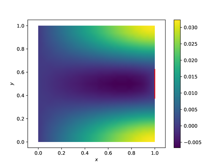
Figure 1: The discrete solution after 8 adaptive refinements. The contact region on the rightmost boundary is highlighted in red.

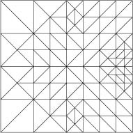
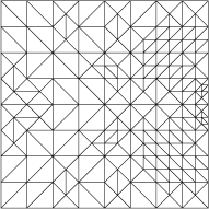
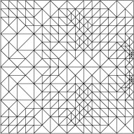
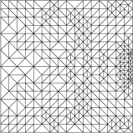
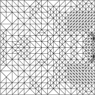
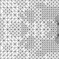
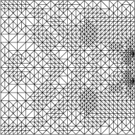
Figure 2: The initial mesh and the resulting sequence of adaptively refined meshes.

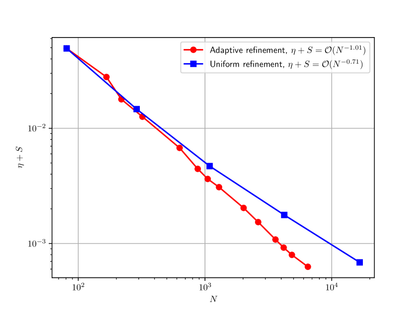
Figure 3: Convergence of the error estimator $\eta+S$ as a function of the number of degrees of freedom $N$ for the uniform and the adaptive mesh sequences. The observed approximate convergence rates are given in the text box window.

References

- [1] S. Auliac, Z. Belhachmi, F. Ben Belgacem, and F. Hecht, Quadratic finite elements with non matching grids for the unilateral boundary contact, ESAIM: Math. Model. Numer. Anal., 47 (2013), pp. 1185–1205.
- [2] Z. Belhachmi and F. Ben Belgacem, Quadratic finite element approximation of the Signorini problem, Math. Comp., 72 (2003), pp. 83–104.
- [3] F. Ben Belgacem, Numerical simulation of some variational inequalities arisen from unilateral contact problems by the finite element method, SIAM J. Numer. Anal., 37 (2000), pp. 1198–1216.
- [4] F. Ben Belgacem and Y. Renard, Hybrid finite element methods for the Signorini problem, Math. Comp., 72 (2003), pp. 1117–1145.
- [5] H. Blum and F. Suttmeier, An adaptive finite element discretization for a simplified Signorini problem, Calcolo, 37 (2000), pp. 65–77.
- [6] F. Brezzi, W. W. Hager, and P.-A. Raviart, Error estimates for the finite element solution of variational inequalities. II. Mixed methods, Numer. Math., 31 (1978/79), pp. 1–16.
- [7] E. Burman, P. Hansbo, and M. G. Larson, The penalty-free Nitsche method and nonconforming finite elements for the Signorini problem, SIAM J. Numer. Anal., 55 (2017), pp. 2523–2539.
- [8] F. Chouly, M. Fabre, P. Hild, R. Mlika, J. Pousin, and Y. Renard, An overview of recent results on Nitsche’s method for contact problems, in Geometrically Unfitted Finite Element Methods and Applications, S. Bordas, E. Burman, M. Larson, and M. Olshanskii, eds., vol. 121 of Lecture Notes in Computational Science and Engineering, Springer, 2018, pp. 93–141.
- [9] F. Chouly, M. Fabre, P. Hild, J. Pousin, and Y. Renard, Residual-based a posteriori error estimation for contact problems approximated by Nitsche’s method, IMA J. Numer. Anal., 38 (2018), pp. 921–954.
- [10] F. Chouly and P. Hild, A Nitsche-based method for unilateral contact problems: numerical analysis, SIAM J. Numer. Anal., 51 (2013), pp. 1295–1307.
- [11] F. Chouly, P. Hild, and Y. Renard, Symmetric and non-symmetric variants of Nitsche’s method for contact problems in elasticity: theory and numerical experiments, Math. Comp., 84 (2015), pp. 1089–1112.
- [12] G. Drouet and P. Hild, Optimal convergence for discrete variational inequalities modelling Signorini contact in 2D and 3D without additional assumptions on the unknown contact set, SIAM J. Numer. Anal., 53 (2015), pp. 1488–1507.
- [13] R. S. Falk, Error estimates for the approximation of a class of variational inequalities, Math. Comp., 28 (1974), pp. 963–971.
- [14] T. Gustafsson, R. Stenberg, and J. Videman, Error analysis of Nitsche’s mortar method. Submitted. arXiv preprint:1802.10430.
- [15] , A stabilised finite element method for the plate obstacle problem. Submitted. arXiv preprint:1711.04166.
- [16] , Mixed and stabilized finite element methods for the obstacle problem, SIAM J. Numer. Anal., 55 (2017), pp. 2718–2744.
- [17] , On finite element formulations for the obstacle problem – mixed and stabilised methods, Comput. Methods Appl. Math, 17 (2017), pp. 413–429.
- [18] , An adaptive finite element method for the inequality-constrained Reynolds equation, Comput. Methods Appl. Mech. Engrg., 336 (2018), pp. 156–170.
- [19] J. Haslinger, I. Hlaváček, and J. Nečas, Numerical methods for unilateral problems in solid mechanics, in Handbook of numerical analysis, Vol. IV, Handb. Numer. Anal., IV, North-Holland, Amsterdam, 1996, pp. 313–485.
- [20] J. Haslinger and J. Lovíšek, Quadratic finite element methods for unilateral contact problems, Comment. Math. Univ. Carolin., 21 (1980), pp. 231–246.
- [21] P. Hild and S. Nicaise, A posteriori error estimations of residual type for Signorini’s problem, Numer. Math., 101 (2005), pp. 523–549.
- [22] , Residual a posteriori error estimators for contact problems in elasticity, M2AN Math. Model. Numer. Anal., 41 (2007), pp. 897–923.
- [23] P. Hild and Y. Renard, An improved a priori error analysis for finite element approximations of Signorini’s problem, SIAM J. Numer. Anal., 50 (2012), pp. 2400–2419.
- [24] I. Hlaváček, J. Haslinger, J. Nečas, and J. Lovíšek, Solution of Variational Inequalities in Mechanics, vol. 66 of Applied Mathematical Sciences, Springer-Verlag, New York, 1988.
- [25] N. Kikuchi and J. T. Oden, Contact Problems in Elasticity: A Study of Variational Inequalities and Finite Element Methods, SIAM, Philadelphia, 1988.
- [26] D. Kinderlehrer and G. Stampacchia, An Introduction to Variational Inequalities and Their Applications, Academic Press, New York-London, 1980.
- [27] R. Krause, A. Veeser, and M. Walloth, An efficient and reliable residual-type a posteriori error estimator for the Signorini problem, Numer. Math., 130 (2015), pp. 151–197.
- [28] M. Moussaoui and K. Khodja, Régularité des solutions d’un problème mêlé Dirichlet-Signorini dans un domaine polygonal plan, Commun. Part. Diff. Eq., 17 (1992), pp. 805–826.
- [29] F. Scarpini and M. Vivaldi, Error estimates for the approximation of some unilateral problems, RAIRO Anal. Numér., 11 (1977), pp. 197–208.
- [30] A. Schröder, Error control in h- and hp-adaptive FEM for Signorini’s problem, J. Numer. Math., 17 (2009), pp. 299–318.
- [31] , Mixed finite element methods of higher-order for model contact problems, SIAM J. Numer. Anal., 49 (2011), pp. 2323–2339.
- [32] R. Stenberg, On some techniques for approximating boundary conditions in the finite element method, J. Comput. Appl. Math., 63 (1995), pp. 139–148.
- [33] L. Tartar, Introduction to Sobolev Spaces and Interpolation Theory, Springer Berlin-Heidelberg, 2007.
- [34] R. Verfürth, A Posteriori Error Estimation Techniques for Finite Element Methods, Oxford University Press, Oxford, 2013.
- [35] A. Weiss and B. Wohlmuth, A posteriori error estimator and error control for contact problems, Math. Comp., 78 (2009), pp. 1237–1267.
- [36] B. Wohlmuth, Variationally consistent discretization schemes and numerical algorithms for contact problems, Acta Numerica, 20 (2011), pp. 569–734.