Breaking the fundamental energy dissipation limit in ferroelectric-dielectric capacitors

Abstract

Half of the energy is always lost when charging a capacitorSalahuddin and Datta (2007). Even in the limit of vanishing resistance, half of the charging energy is still lost—to radiation instead of heat. While this fraction can technically be reduced by charging adiabatically, it otherwise places a fundamental limit on the charging efficiency of a capacitor. Here we show that this $1/2$ limit can be broken by coupling a ferroelectric to the capacitor dielectric. Maxwell’s equations are solved for the coupled system to analyze energy flow from the perspective of Poynting’s theorem and show that (1) total energy dissipation is reduced below the fundamental limit during charging and discharging; (2) energy is saved by “recycling” the energy already stored in the ferroelectric phase transition; and (3) this phase transition energy is directly transferred between the ferroelectric and dielectric during charging and discharging. These results demystify recent worksRusu et al. (2010); Islam Khan et al. (2011); Lee et al. (2013); Appleby et al. (2014); Khan et al. (2014); Lee et al. (2015); Khan et al. (2016); Zubko et al. (2016) on low energy negative capacitance devices as well as lay the foundation for improving fundamental energy efficiency in all devices that rely on energy storage in electric fields.

Ferroelectrics have recently been shown to exhibit a negative capacitance effect Salahuddin and Datta (2008); Islam Khan et al. (2011); Zubko et al. (2016) when placed in a series combination with a dielectric film. Under appropriate conditions, the dielectric leads to a strong depolarization field that forces the ferroelectric into its normally unstable near-zero polarization states. These results have garnered considerable interest in ferroelectric negative capacitance due to its potential to reduce power consumption below thermodynamic limits in electronic devicesSalahuddin and Datta (2008). In field-effect transistors, for example, negative capacitance has been proposed as a solution to end the “Boltzmann tyranny” on subthreshold swingSalahuddin and Datta (2008); Zhirnov and Cavin (2008); Theis and Solomon (2010). However, negative capacitance has traditionally been understood to require a source (e.g. a battery) that supplies extra energyJonscher (1986). This begs the following question: if extra energy must be supplied by some source, then where is the energy coming from in ferroelectric negative capacitance and is any energy truly saved?

To answer this question, we considered energy flow during charging and discharging of a ferroelectric-dielectric capacitor. We solved Maxwell’s equations for the coupled system and used Poynting’s theorem to show how energy flows. We performed our analysis in the limit of zero resistance in order to understand the fundamental charging and discharging energy costs. The results are shown schematically in Fig. 1a.

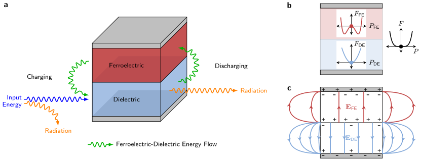
Figure 1: Paths of energy flow during charging and discharging of a capacitor with a ferroelectric. (a) Schematic of energy flow paths during charging (left) and discharging (right) of a ferroelectric-dielectric capacitor. New paths of energy flow emerge between the ferroelectric and dielectric during charging and discharging. These paths are not present in conventional dielectric capacitors. (b) Energy landscapes in a ferroelectric-dielectric capacitor. If the dielectric is sufficiently thick, then its energy landscape $F_{\text{DE}}$ will dominate the energy landscapes $F_{\text{FE}}$ and $F$ of the ferroelectric and overall system respectively. The dielectric polarization $P_{\text{DE}}$ then forces the ferroelectric near its phase transition at zero polarization ($P_{\text{FE}}=0$) via a strong depolarization field. This puts the ferroelectric into a higher energy state in which energy can be extracted from the phase transition. (c) Schematic of the total electric fields in a ferroelectric-dielectric capacitor. When an external electric field is applied, the ferroelectric and dielectric both polarize by different amounts, resulting in a depolarization field. Since the ferroelectric is stabilized in a higher energy state near zero polarization, it releases energy when polarized. This extra energy contributes towards further strengthening the depolarization field, which subsequently further polarizes and charges the dielectric. The resultant electric fields $\mathbf{E}_{\text{FE}}$ and $\mathbf{E}_{\text{DE}}$ in the ferroelectric and dielectric respectively end up pointing in opposite directions.

During charging, input energy flows from an energy source to the dielectric, and a fraction of that energy is dissipated. This dissipation is dominated by electromagnetic radiation in the limit of zero resistance. Notice that there is an additional path of energy flow from the ferroelectric to the dielectric that is not present during charging in conventional capacitors. This implies that the ferroelectric is supplying extra energy to the dielectric. During discharging, the dielectric acts as the energy source and normally dissipates all of its energy when in a conventional capacitor. However, there is a new path of energy flow that allows the dielectric to transfer a fraction of its energy back to the ferroelectric. Thus, we see schematically how energy may be internally recycled in the coupled ferroelectric-dielectric system. However, it is still unclear where the extra energy comes from and how it transfers between the ferroelectric and dielectric.

The origin of this extra energy can be understood from a thermodynamic perspective as shown in Fig. 1b. Due to their phase transition, ferroelectrics possess a higher energy, zero polarization state in their energy landscape. This is in contrast to dielectrics, which have a minimum in their energy landscape at zero polarization. Consequently, coupling a ferroelectric to a dielectric results in a large divergence in polarization at the interface. This establishes a strong depolarization field that stabilizes the ferroelectric near its unstable zero polarization state. The net effect is an electrically-induced transition towards a phase of higher crystal symmetry and can be thought of as an effective shift in the phase transition temperature Salahuddin and Datta (2008); Zubko et al. (2016). This electrical influence is in conflict with the natural temperature-induced transition towards lower crystal symmetry. Thus, we can electrically extract energy from the phase transition by modulating this conflict with an applied electric field. The extracted energy is then transferred between the ferroelectric and dielectric via propagation of the depolarization field as shown schematically in Fig. 1c. Notice that the electric field points in opposite directions from the ferroelectric-dielectric interface due to the negative permittivity of the ferroelectric near its phase transition. It is worth noting that this result was directly obtained from our calculations without any consideration a priori of negative electric susceptibilities or capacitances.

For our quantitative analysis, we modelled the coupled ferroelectric-dielectric system using the electric Gibbs free energy (which we will refer to as simply free energy for the remainder of this letter):

$$G=\int\left(f-\mathbf{E}\cdot\mathbf{P}\right)\,d^{3}r$$ (1)

$f$ is the Helmholtz free energy density as a function of temperature and polarization $\mathbf{P}$; and $\mathbf{E}$ is electric field. Note that $f$, $\mathbf{E}$, and $\mathbf{P}$ all vary with position $\mathbf{r}$, and the functional form of $f$ depends on the material energy landscape. The dielectric was modelled as a linear dielectric, and its electric susceptibility and thickness were normalized as a single tuning parameter. The ferroelectric energy landscape was modelled after Pb(Zr_0.52Ti_0.48)O₃ using Landau-Devonshire phenemonological parametersRabe et al. (2007). We could have used Ginzburg-Landau theory to take into account slow spatial variations in the polarization. However, such fine details would simply add finer spatial variations to our calculated energy flow; the overall flow would remain the same as long as the ferroelectric was still locally stabilized near its zero polarization state. We also assumed a one-dimensional order parameter since polarization is expected to lie primarily along the capacitor axis. Finally, we solved for the stationary states of the coupled ferroelectric-dielectric system by minimizing the free energy with respect to small polarization fluctuations $\delta\mathbf{P}$ under constant electric field and isothermal conditions.

The dynamics of the system were described with Poynting’s theorem:

$$\frac{\partial u}{\partial t}+\nabla\cdot\mathbf{S}=-\mathbf{J}\cdot\mathbf{E}$$ (2)

The internal energy density $u$ inside the ferroelectric and dielectric was determined by solving for the states of the coupled ferroelectric-dielectric system (as described in the previous paragraph). The form of the Poynting vector $\mathbf{S}$ was obtained by solving Maxwell’s equations using retarded scalar and vector potentials. For ease of calculation, we considered a simple wire loop geometry containing a voltage source and the ferroelectric-dielectric capacitor at diametrically opposite positions. With $u$ and $\mathbf{S}$, it is possible to numerically solve the differential equation (2) and compute the power supplied and consumed over time as shown in Fig. 2a-b.

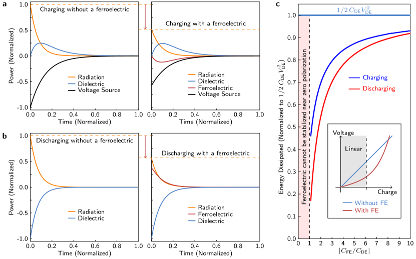
Figure 2: Power comparison during charging and discharging of a capacitor without/with a ferroelectric. Negative power corresponds to power supplied. (a) Power versus time during charging of a capacitor without a ferroelectric (left) and with a ferroelectric added (right). The ferroelectric and dielectric parameters are set such that $|C_{\text{FE}}/C_{\text{DE}}|=2$ (see (c) and Fig. 3 for more information) where $C_{\text{FE}}$ is the ferroelectric capacitance, and $C_{\text{DE}}$ is the dielectric capacitance. The voltage source supplies less power when the ferroelectric is coupled to the dielectric, and the amount of power radiated is reduced. The dielectric still receives the same amount of energy because the ferroelectric supplies the missing power. (b) Power versus time during discharging of the same capacitors from (a) (without a ferroelectric, left; and with a ferroelectric, right). The dielectric acts as the source during discharging, and a fraction of its power is delivered to the ferroelectric instead of completely radiating away as in the conventional case. (c) Total energy dissipated as a function of the capacitance matching $|C_{\text{FE}}/C_{\text{DE}}|$ after charging and discharging. The energy is normalized to $1/2\,C_{\text{DE}}V_{\text{DE}}^{2}$, which is the conventional amount of energy dissipated without a ferroelectric. The inset shows that the capacitor becomes nonlinear when a ferroelectric is added, resulting in charge-dependent energy dissipation. The curves shown here were calculated by charging to and discharging from the end of the linear region.

During charging (Fig. 2a), less power is supplied by the energy source when a ferroelectric is coupled to the dielectric, and less power is lost to radiation. However, the dielectric still receives the same amount of energy, and we find that the ferroelectric supplies the missing part using the energy stored in its phase transition. During discharging (Fig. 2b), the dielectric radiates energy, but the ferroelectric appears to “capture” a fraction of it back to replenish its phase transition energy when coupled to the dielectric. The total energy dissipated is shown in Fig. 2c as a function of the “capacitance matching” between the ferroelectric and dielectric. We find that the amount of energy dissipated is reduced below the conventional $1/2\,CV^{2}$ during charging and discharging, and it is minimized when the ferroelectric and dielectric capacitances are equal (i.e. $|C_{\text{FE}}/C_{\text{DE}}|\to 1$). It should be noted that the capacitor becomes nonlinear when a ferroelectric is added (inset of Fig. 2c), resulting in charge-dependent energy dissipation. We charged to the end of the linear region and then discharged completely to calculate the curves in Fig. 2c.

The capacitance matching can be better understood by examining the energy landscapes shown in Fig. 3a.

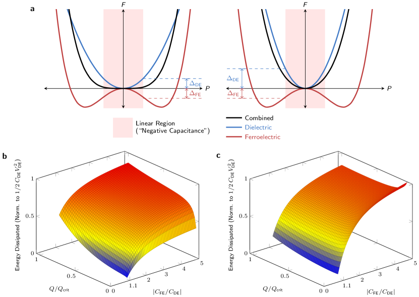
Figure 3: Energy balancing and capacitance matching. (a) Energy landscapes showing perfect energy balancing $\Delta_{\text{DE}}\approx\Delta_{\text{FE}}$ (left) and imperfect energy balancing $\Delta_{\text{DE}}>\Delta_{\text{FE}}$ (right) between the ferroelectric and dielectric. Even with perfect energy balancing, the ferroelectric eventually runs out of energy stored in its phase transition. This occurs at the end of the linear region, after which point the ferroelectric can no longer supply energy to the dielectric and must receive energy from an external source to continue polarizing. (b) Total energy dissipated as a function of the capacitance matching $|C_{\text{FE}}/C_{\text{DE}}|$ after storing charge $Q$ on the capacitor plates. $C_{\text{FE}}$ is the ferroelectric capacitance, and $C_{\text{DE}}$ is the dielectric capacitance. The energy dissipated is normalized to $1/2\,C_{\text{DE}}V_{\text{DE}}^{2}$, which is the energy conventionally dissipated without a ferroelectric. $Q_{\text{crit}}$ is the charge corresponding to the end of the linear region. (c) Total energy dissipated as a function of the capacitance matching $|C_{\text{FE}}/C_{\text{DE}}|$ after discharging $Q$ amount of charge.

In the left set of landscapes, the energy available in the ferroelectric phase transition closely matches the energy “needs” of the dielectric in the linear region. This allows the ferroelectric to supply nearly all of the energy needed to charge the dielectric. Consequently, minimal additional energy is needed from an external source, and less energy will be lost to radiation while propagating from the source to the dielectric. This is an example of perfect energy balancing. In contrast, the right half of Fig. 3a shows an example of poor energy balancing. The energy available in the ferroelectric is insufficient for charging the dielectric. Consequently, more energy is needed from an external source, and more energy will be lost to radiation while propagating to the dielectric. We can control the energy balancing by tuning the energy landscapes. This is accomplished by changing film thickness or electric susceptibility (e.g. by changing temperature or strain; or using different materials). Since these parameters directly affect the system’s capacity to store energy in an electric field, the energy balancing can be thought of as a capacitance matching between the ferroelectric and dielectric. In the linear region, for example, the ferroelectric capacitance is negative due to the negative curvature of the energy landscape and should be equal and opposite to the dielectric capacitance for proper matching. The ferroelectric is able to supply energy to the dielectric within this linear region. However, it will eventually run out of stored energy and begin requiring energy from an external source to continue polarizing. This is reflected by the change in the energy landscape’s curvature from negative to positive at the end of the linear region. This is also reflected in the charge dependency of the energy dissipation as shown in Fig. 3b-c. No matter how perfectly matched the ferroelectric and dielectric are, the energy dissipation increases for greater amounts of charge during both charging (Fig. 3b) and discharging (Fig. 3c).

Finally, we explicitly show how energy transfers between the ferroelectric and dielectric by computing the Poynting vector at various positions in and around the system. The overall energy flow during charging is shown schematically in Fig. 4a.

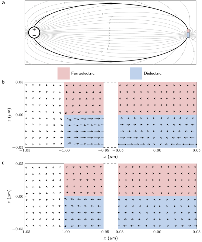
Figure 4: Poynting vector calculations. (a) Schematic of overall energy flow from the source to the ferroelectric-dielectric capacitor during charging. (b) Poynting vector field along the side of the capacitor and near the center during charging. $x$ is the in-plane spatial coordinate, and $z$ is the spatial coordinate along the capacitor axis. (c) Poynting vector field along the side of the capacitor and near the center during discharging.

Notice that energy flows from the source to the ferroelectric-dielectric system, but some of it radiates away. If we zoom in on the capacitor (Fig. 4b), we see that energy flows directly from the ferroelectric to the dielectric through the surrounding space. The Poynting vector diverges outwards (energy is decreasing) at the center of the ferroelectric and inwards (energy is increasing) at the dielectric center. During discharging (Fig. 4c), the Poynting vector diverges oppositely compared to the charging case. The dielectric acts as the source with some of its energy flowing into the ferroelectric through the surrounding space while the remainder radiates away.

In conclusion, we have shown that it is possible to improve upon the otherwise fundamental limit on energy dissipation of $1/2\,CV^{2}$ during charging and discharging of a capacitor by coupling a ferroelectric to the dielectric. We used a thermodynamic model to show that the dielectric can stabilize the ferroelectric near its phase transition, enabling extraction of the energy stored in the phase transition. Poynting’s theorem and Maxwell’s equations then explicitly showed that this stored energy directly flows between the ferroelectric and dielectric during charging and discharging. The net result is a reduction in total energy dissipation below the conventional limit. This reduction can be maximized by balancing the energy stored in the ferroelectric phase transition with the energy needed by the dielectric. These results provide the framework for understanding and improving fundamental energy efficiency in all devices that operate on storing energy in electric fields.

Appendix A Poynting’s Theorem

Poynting’s theorem is a statement of conservation of energy for a system of charged particles and can be written as a differential continuity equation as given in (2). The integral form is

$$\int_{\Omega}\left(\frac{\partial u}{\partial t}+\nabla\cdot\mathbf{S}\right)\,d^{3}r=-\int_{\Omega}(\mathbf{J}\cdot\mathbf{E})\,d^{3}r$$ (3)

where the volume $\Omega$ can be arbitrary, but we take it as the volume filled by the components of the circuit to establish appropriate boundary conditions. This differential equation can be numerically solved for the current density $\mathbf{J}$ if the remaining variables can be expressed in terms of current density. We accomplish this by establishing a consistent relationship between internal energy density $u$ and electric field $\mathbf{E}$ for a given current density. First, an initial electric field is assumed, and the state of the ferroelectric-dielectric system is determined by minimizing the free energy in (1) with respect to small polarization fluctuations. This determines the ferroelectric and dielectric polarization states, which allow us to determine the internal energy density $u$ and charge density $\rho$. This charge density can be used in conjunction with a given current density to solve Maxwell’s equations by determining the retarded scalar and vector potentials:

$$V(\mathbf{r},t)=\\ \frac{1}{4\pi\epsilon_{0}}\int\frac{\rho(\mathbf{r}^{\prime},t^{\prime})}{|\mathbf{r}-\mathbf{r}^{\prime}|}\delta\left(t^{\prime}-t+\frac{|\mathbf{r}-\mathbf{r}^{\prime}|}{c}\right)\,dt^{\prime}\,d^{3}r^{\prime}$$ (4)

$$\mathbf{A}(\mathbf{r},t)=\\ \frac{\mu_{0}}{4\pi}\int\frac{\mathbf{J}(\mathbf{r}^{\prime},t^{\prime})}{|\mathbf{r}-\mathbf{r}^{\prime}|}\delta\left(t^{\prime}-t+\frac{|\mathbf{r}-\mathbf{r}^{\prime}|}{c}\right)\,dt^{\prime}\,d^{3}r^{\prime}$$ (5)

The solutions to Maxwell’s equations are then

$$\mathbf{E}(\mathbf{r},t) =-\nabla V-\frac{\partial\mathbf{A}}{\partial t}$$ (6)

$$\mathbf{B}(\mathbf{r},t) =\nabla\times\mathbf{A}$$ (7)

To reduce numerical error, we directly solved Maxwell’s equations by analytically combining (4)-(7) and evaluating the resulting Jefimenko’s equations. Notice that the electric field computed here must be equal to the electric field initially assumed when determining the internal energy density. Thus, the electric field and internal energy density must be solved for consistently, and this can be accomplished for a given current density. From (5) and (7), the magnetic field $\mathbf{B}$ only depends on current density, so the Poynting vector $\mathbf{S}$ can also be computed for a given current density:

$$\mathbf{S}=\frac{\mathbf{E}\times\mathbf{B}}{\mu_{0}}$$ (8)

The only remaining unknown quantity is the current density, which can now be solved for using Poynting’s theorem.