Density Forecasts in Panel Data Models:
A Semiparametric Bayesian Perspective

Abstract

This paper constructs individual-specific density forecasts for a panel of firms or households using a dynamic linear model with common and heterogeneous coefficients as well as cross-sectional heteroskedasticity. The panel considered in this paper features a large cross-sectional dimension $N$ but short time series $T$. Due to the short $T$, traditional methods have difficulty in disentangling the heterogeneous parameters from the shocks, which contaminates the estimates of the heterogeneous parameters. To tackle this problem, I assume that there is an underlying distribution of heterogeneous parameters, model this distribution nonparametrically allowing for correlation between heterogeneous parameters and initial conditions as well as individual-specific regressors, and then estimate this distribution by combining information from the whole panel. Theoretically, I prove that in cross-sectional homoskedastic cases, both the estimated common parameters and the estimated distribution of the heterogeneous parameters achieve posterior consistency, and that the density forecasts asymptotically converge to the oracle forecast. Methodologically, I develop a simulation-based posterior sampling algorithm specifically addressing the nonparametric density estimation of unobserved heterogeneous parameters. Monte Carlo simulations and an empirical application to young firm dynamics demonstrate improvements in density forecasts relative to alternative approaches.

JEL Codes: C11, C14, C23, C53, L25

Keywords: Bayesian, Semiparametric Methods, Panel Data, Density Forecasts, Posterior Consistency, Young Firm Dynamics

1 Introduction

Panel data, such as a collection of firms or households observed repeatedly for a number of periods, are widely used in empirical studies. It can also be useful for forecasting individuals’ future outcomes, which is interesting and important in many applications, for example, PSID for income dynamics (Hirano, 2002; Gu and Koenker, 2017b) and bank balance sheet data for bank stress tests (Liu et al., 2020). This paper constructs individual-specific density forecasts using a dynamic linear panel data model with common and heterogeneous coefficients as well as cross-sectional heteroskedasticity.

In this paper, I consider young firm dynamics as the empirical application. For illustrative purposes, consider a simple dynamic panel data model as the baseline setup:

$$\underset{\text{performance}}{\underbrace{y_{it}}}=\beta y_{i,t-1}+\underset{\text{skill}}{\underbrace{\lambda_{i}}}+\underset{\text{shock}}{\underbrace{u_{it}}},\quad u_{it}\sim N\left(0,\sigma^{2}\right),$$ (1)

where $i=1,\cdots,N$, and $t=1,\cdots,T+1$. $y_{it}$ is the observed firm performance such as log employment, $\lambda_{i}$ is the unobserved skill of an individual firm, and $u_{it}$ is an i.i.d.  shock. Skill is independent of the shock, and the shock is independent across firms and times. $\beta$ and $\sigma^{2}$ are common across firms, where $\beta$ represents the persistence of the dynamic pattern and $\sigma^{2}$ gives the size of the shocks. Based on the observed panel from period $0$ to period $T$, I am interested in forecasting the future performance of any specific firm in period $T+1$.

The panel considered in this paper features a large cross-sectional dimension $N$ but short time series $T$. For instance, the number of observations for each young firm is restricted by its age. Good estimates of the unobserved skill $\lambda_{i}$ facilitate good forecasts of $y_{i,T+1}$. Because of the short $T$, traditional methods have difficulty in disentangling the unobserved skill $\lambda_{i}$ from the shock $u_{it}$, which contaminates the estimates of $\lambda_{i}$, even if $N$ goes to infinity.

To tackle this problem, I assume that $\lambda_{i}$ is drawn from an underlying skill distribution $f$ and estimate this distribution by combining information from the whole panel. In terms of modeling $f$, the parametric Gaussian density misses many features in real-world data, such as asymmetry, heavy tails, and multiple peaks. For example, as good ideas are scarce, the skill distribution of young firms may be highly skewed. This calls for a flexible modeling of $f$, and here I estimate $f$ via a nonparametric Bayesian approach where the prior is constructed from a mixture model and allows for correlation between $\lambda_{i}$ and the initial condition $y_{i0}$ (i.e. a correlated random effects model).

Conditional on $f$, we can treat it as a prior distribution and combine it with firm-specific data to obtain the firm-specific posterior via Bayes’ theorem. In a special case where the common parameters are $\left(\beta,\sigma^{2}\right)=\left(0,1\right)$, the firm-specific posterior is

$$p\left(\lambda_{i}\left|f,y_{i,0:T}\right.\right) =\frac{p\left(\left.y_{i,1:T}\right|\lambda_{i}\right)f\left(\lambda_{i}\left|y_{i0}\right.\right)}{\int p\left(\left.y_{i,1:T}\right|\lambda_{i}\right)f\left(\lambda_{i}\left|y_{i0}\right.\right)d\lambda_{i}}.$$

This firm-specific posterior helps better infer the firm-specific unobserved skill $\lambda_{i}$ and better forecast the firm-specific future performance, thanks to the estimated underlying distribution $f$ that integrates the information from the whole panel in an efficient and flexible way. This is only an intuitive explanation of why the skill distribution $f$ is crucial. In the actual implementation, the correlated random effect distribution $f$, common parameters $\left(\beta,\sigma^{2}\right)$, and firm-specific skill $\lambda_{i}$ are all inferred simultaneously.

It is natural to construct density forecasts based on the firm-specific posterior. In general, forecasting can be done in a point, interval, or density manner, with density forecasts giving the richest insight into future outcomes. By definition, a density forecast provides a predictive distribution of firm $i$’s future performance and summarizes all sources of uncertainties; hence, it is preferable in the context of young firm dynamics and other applications with large uncertainties and nonstandard distributions. In particular, for the baseline model in (1), the density forecasts reflect uncertainties arising from the future shock $u_{i,T+1}$, unobserved individual heterogeneity $\lambda_{i}$, and estimation uncertainty of common parameters $\left(\beta,\sigma^{2}\right)$ and of skill distribution $f$. Moreover, once density forecasts are obtained, one can easily recover point and interval forecasts.

The contributions of this paper are threefold. First, I establish the theoretical properties of the proposed predictor when the cross-sectional dimension $N$ tends to infinity. To begin, I provide conditions for identifying the common parameters and the distribution of the individual heterogeneity in both cross-sectional homoskedastic and heteroskedastic models. Then, I prove that the proposed estimator achieves posterior consistency in cross-sectional homoskedastic cases. Compared with previous literature on posterior consistency in density estimation problems, there are several challenges in the panel data framework: (1) a deconvolution problem disentangling unobserved individual effects and shocks, (2) an unknown common shock size in cross-sectional homoskedastic cases, (3) strictly exogenous and predetermined variables (including lagged dependent variables) as covariates, and (4) correlated random coefficients addressed by flexible conditional density estimation. Based on the posterior consistency of the estimates, the discrepancy between the proposed density predictor and the oracle is arbitrarily small asymptotically. The oracle predictor is an (infeasible) benchmark defined as the individual-specific posterior predictive distribution, assuming known common parameters and a known distribution of the heterogeneous parameters.

Second, I develop a posterior sampling algorithm specifically addressing nonparametric density estimation of the unobserved individual effects. For a random coefficients model, which is a special case where the individual effects are independent of the conditioning variables, the $f$ part becomes an unconditional density estimation problem. I adopt a Dirichlet Process Mixture (DPM) prior for $f$ and construct a posterior sampler building on the blocked Gibbs sampler proposed by Ishwaran and James (2001, 2002). For a correlated random coefficients model, I further adapt the proposed algorithm to the much harder conditional density estimation problem using a probit stick-breaking process prior suggested by Pati et al. (2013).

Third, Monte Carlo simulations demonstrate improvement in density forecasts relative to alternative predictors with various parametric priors on $f$, evaluated by the log predictive score. An application to young firm dynamics also shows that the proposed predictor provides more accurate density predictions. The better forecasting performance is largely due to three key features (in order of importance): the nonparametric Bayesian prior, cross-sectional heteroskedasticity, and correlated random coefficients. The estimated model also helps shed light on the latent heterogeneity structure of firm-specific coefficients and cross-sectional heteroskedasticity, as well as whether and how the unobserved heterogeneity depends on the initial condition of the firms.

Moreover, the proposed method is applicable beyond forecasting. Here estimating heterogeneous parameters is important because we want to generate good individual-specific forecasts, but in other cases, the heterogeneous parameters themselves could be the objects of interest. For example, the technique developed here can be adapted to infer individual-specific treatment effects.

Related Literature

First, this paper contributes to the literature on individual forecasts in a panel data setup, and is closely related to Liu et al. (2020) and Gu and Koenker (2017a, b). Liu et al. (2020) focus on point forecasts. They utilize the idea of Tweedie’s formula to steer away from the complicated deconvolution problem in estimating $\lambda_{i}$ and establish the ratio optimality of point forecasts. Unfortunately, the Tweedie shortcut is not applicable to the inference of the underlying $\lambda_{i}$ distribution and therefore not suitable for density forecasts. In addition, this paper addresses cross-sectional heteroskedasticity where $\sigma_{i}^{2}$ is an unobserved random quantity, while Liu et al. (2020) incorporate cross-sectional and time-varying heteroskedasticity via a deterministic function of observed conditioning variables.

Gu and Koenker (2017b) address the density estimation problem, but with a different method. This paper infers the underlying $\lambda_{i}$ distribution via a full Bayesian approach (i.e.  adopting a prior on the $\lambda_{i}$ distribution and updating the prior belief by the observed data), whereas they employ an empirical Bayes approach (i.e.  choosing the $\lambda_{i}$ distribution by maximizing the marginal likelihood of data). In principle, the full Bayesian approach is preferable for density forecasts, as it captures all sources of uncertainties, including estimation uncertainty of the underlying $\lambda_{i}$ distribution, which has been omitted by the empirical Bayes approach. In addition, this paper features correlated random coefficients allowing the cross-sectional heterogeneity to interact with the initial conditions, whereas Gu and Koenker (2017b) focus on random effects models without this interaction.

In their recent paper, Gu and Koenker (2017a) also compare their method with an alternative semiparametric Bayesian estimator featuring a Dirichlet Process (DP) prior under a set of fixed scale parameters. There are two major differences between their DP setup and the DPM prior used in this paper. First, the DPM prior provides continuous individual effect distributions, which could be the case in many empirical setups. Second, unlike their set of fixed scale parameters, this paper incorporates a hyperprior for the scale parameter and updates it via the observed data, hence let the data choose the complexity of the mixture approximation, which can essentially be viewed as an “automatic” model selection.

Earlier works on full Bayesian analyses with parametric priors on $\lambda_{i}$ can be found in Lancaster (2002) (orthogonal reparametrization and a flat prior); Chamberlain and Hirano (1999), Chib and Carlin (1999), and Sims (2000) (Gaussian prior); and Chib (2008) (student-t and finite mixture priors). There have also been empirical works on the DPM model with panel data, but they mostly focus on empirical studies rather than theoretical analyses. For example, Hirano (2002) and Fisher and Jensen (2021) use linear panel models with setups different from this paper. Hirano (2002) considers flexibility in the $u_{it}$ distribution instead of the $\lambda_{i}$ distribution. Fisher and Jensen (2021) assume random effects instead of correlated random effects. Burda and Harding (2013) and Rossi (2014) use a panel probit model and a panel logit model, respectively.

In the frequentist literature, Li and Vuong (1998), Delaigle et al. (2008), Evdokimov (2010), and Hu (2017), among others, have studied a similar deconvolution problem and estimated the $\lambda_{i}$ distribution. Also see Compiani and Kitamura (2016) for a review of frequentist applications of mixture models. However, the frequentist approach misses estimation uncertainty, which matters in density forecasts, as mentioned previously.

Second, this paper also relates to the literature on nonparametric Bayesian methods in density estimation problems (Ghosh and Ramamoorthi, 2003; Hjort et al., 2010; Ghosal and van der Vaart, 2017). In particular, for unconditional density estimation, a recent paper by Canale and De Blasi (2017) relaxed the tail conditions to accommodate multivariate location-scale mixtures. For conditional density estimation, the mixing probabilities can be characterized by a multinomial choice model (Norets, 2010; Norets and Pelenis, 2012), a kernel stick-breaking process (Norets and Pelenis, 2014; Pelenis, 2014; Norets and Pati, 2017), or a probit stick-breaking process (Pati et al., 2013). I adopt the Pati et al. (2013) approach and establish posterior consistency for a multivariate conditional density estimator featuring infinite location-scale mixtures with a probit stick-breaking process.

To account for deconvolution, I construct an inversion inequality that links the convergence of the distribution of observables to the convergence of the distribution of the unobserved individual heterogeneity. The latter is in the Wasserstein metric, which is useful in handling deconvolution problems as found in the recent literature. For example, Nguyen (2013) considers the unobserved distribution on a discrete support, and Su et al. (2020) flexibly model a symmetric unimodal unobserved distribution using a mixture of symmetric uniforms where the bounds are drawn from a Dirichlet process location-mixture of Gammas. Their setups, however, differ from the current framework, which calls for a new inversion inequality developed in this paper. Then, I further take into account the dynamic panel data structure, as well as obtain the convergence of the proposed predictor to the oracle predictor.

Last but not least, the empirical application in this paper also relates to the young firm dynamics literature. Akcigit and Kerr (2018) document that R&D intensive firms grow faster, especially for smaller firms. Robb and Seamans (2014) examine the role of R&D in capital structure and performance of young firms. The empirical analysis of this paper builds on these findings. Besides more accurate density forecasts, I also obtain the latent heterogeneity structure of firm-specific coefficients and cross-sectional heteroskedasticity.

The rest of the paper is organized as follows. Section 2 specifies the general panel data model, density forecasts, and nonparametric Bayesian priors; Section 3 establishes the posterior consistency of the estimates and the convergence of the density forecasts to the oracle; Section 4 conducts Monte Carlo simulations; Section 5 presents the empirical application to young firm dynamics; and Section 6 concludes. Notations, proofs, algorithms, and additional results are in the Appendix.

2 Model

2.1 General Panel Data Model

The general panel data model with (correlated) random coefficients and potential cross-sectional heteroskedasticity can be specified as

$$y_{it}=\beta^{\prime}x_{i,t-1}+\lambda_{i}^{\prime}w{}_{i,t-1}+u_{it},\quad u_{it}\sim N\left(0,\sigma_{i}^{2}\right),$$ (2)

where $i=1,\cdots,N$, and $t=1,\cdots,T+h$. Similar to the baseline setup in (1), $y_{it}$ is the observed individual outcome, such as young firm performance. The main goal of this paper is to estimate the model using the sample from period $0$ to period $T$ and forecast the future distribution of $y_{i,T+h}$ for any individual $i$. In the remainder of the paper, I focus on the case where $h=1$ (i.e.  one-period-ahead forecasts) for notational simplicity, and the discussion can be extended to multi-period-ahead forecasts via either a direct or an iterated approach (Marcellino et al., 2006).

$w_{i,t-1}$ is a vector of observed covariates that have heterogeneous effects on the outcomes, with $\lambda_{i}$ being the unobserved heterogeneous coefficients. $w_{i,t-1}$ is strictly exogenous and captures key sources of individual heterogeneity. If $w_{i,t-1}=1$, $\lambda_{i}$ is reduced to an individual-specific intercept, e.g. firm $i$’s skill level in the baseline model (1). More generally, $w_{i,t-1}$ can contain individual-specific variables (e.g.  firm-specific R&D) and aggregate variables (e.g.  a recession dummy). I focus on the former case below for notational simplicity. In the latter case, all theoretical analyses would be further conditioned on the aggregate observations.

$x_{i,t-1}$ is a vector of observed covariates that have homogeneous effects on the outcomes, and $\beta$ is the corresponding vector of common parameters. I decompose $x_{i,t-1}=\left[x_{i,t-1}^{O\prime},x_{i,t-1}^{P\prime}\right]^{\prime}$, where $x_{i,t-1}^{O}$ is strictly exogenous and $x_{i,t-1}^{P}$ is predetermined. One example of $x_{i,t-1}^{P}$ is the lagged outcome $y_{i,t-1}$ capturing the persistence. Both $x_{i,t-1}^{O}$ and $x_{i,t-1}^{P}$ can include other control variables, such as firm characteristics and general economic conditions. Let $x_{i,t-1}^{P*}$ denote the subgroup of $x_{i,t-1}^{P}$ excluding lagged outcomes, then $x_{i,t-1}=\left[x_{i,t-1}^{O\prime},x_{i,t-1}^{P*\prime},y_{i,t-1}\right]^{\prime}$ with $\beta=\left[\beta^{O\prime},\beta^{P*\prime},\rho\right]^{\prime}$. Here, the distinction between homogeneous effects $\beta^{\prime}x_{i,t-1}$ and heterogeneous effects $\lambda_{i}^{\prime}w_{i,t-1}$ helps model the key latent heterogeneities while avoiding the curse of dimensionality. Combining information from the covariates, the conditioning set at period $t$ is defined as $c_{i,t-1}=\left(x_{i,0:t-1}^{P},x_{i,0:T}^{O},w_{i,0:T}\right).$ We further define $D=\left(\left\{D_{i}\right\}_{i=1}^{N}\right)$, where $D_{i}=c_{iT}$, as the data used for estimation and the conditioning set for posterior inference.

$u_{it}$ is an individual-time-specific shock characterized by zero mean and potential cross-sectional heteroskedasticity $\sigma_{i}^{2}$, with cross-sectional homoskedasticity being a special case where $\sigma_{i}^{2}=\sigma^{2}$. In a unified framework, I denote the common parameters by $\vartheta$, the individual heterogeneity by $h_{i}$, and the underlying distribution of $h_{i}$ by $f$. For instance, $\vartheta=\beta,\;h_{i}=\left(\lambda_{i},\sigma_{i}^{2}\right)$ under cross-sectional heteroskedasticity. In many empirical applications, such as the young firm example, the size of risk may vary over the cross-section, so cross-sectional heteroskedasticity could contribute to better density forecasts.

As stressed in the motivation, the underlying distribution of individual effects is the key to better density forecasts. In the literature, there are usually two types of assumptions on this distribution. One is the random coefficients model, where the individual effects $h_{i}$ are independent of the conditioning variables $c_{i0}=\left(x_{i0}^{P},x_{i,0:T}^{O},w_{i,0:T}\right)$. The other is the correlated random coefficients model, where $h_{i}$ and $c_{i0}$ could be correlated. This paper considers both models while focusing on the latter—although the former is more parsimonious and easier to implement, the latter is more realistic for young firm dynamics as well as many other empirical setups. In practice, it is more feasible to only take into account a subset of $c_{i0}$ or a function of $c_{i0}$ that is relevant for the specific study.

2.2 Oracle and Feasible Predictors

This subsection formally defines the infeasible optimal oracle predictor and the feasible semiparametric Bayesian predictor proposed in this paper. Both definitions rely on the conditional predictor,

$$f_{i,T+1}^{cond}\left(y\left|\vartheta,f,D_{i}\right.\right) =\int\underset{\text{future shock}}{\underbrace{p\left(\left.y\right|h_{i},\vartheta,w_{iT},x_{iT}\right)}}\cdot\underset{\text{individual heterogeneity}}{\underbrace{p\left(h_{i}\left|\vartheta,f,D_{i}\right.\right)}}dh_{i},$$ (3)

which provides the density forecasts of $y_{i,T+1}$ conditional on the common parameters $\vartheta$, underlying distribution $f$, and individual $i$’s data $D_{i}$. The first term $p\left(\left.y\right|h_{i},\vartheta,w_{iT},x_{iT}\right)$ captures individual $i$’s uncertainty due to the future shock $u_{i,T+1}$. The second term

$$p\left(h_{i}\left|\vartheta,f,D_{i}\right.\right)=\frac{\prod_{t=1}^{T}p\left(\left.y_{it}\right|h_{i},\vartheta,w_{i,t-1},x_{i,t-1}\right)f\left(h_{i}\left|c_{i0}\right.\right)}{\int\prod_{t=1}^{T}p\left(\left.y_{it}\right|h_{i},\vartheta,w_{i,t-1},x_{i,t-1}\right)f\left(h_{i}\left|c_{i0}\right.\right)dh_{i}}$$

is the individual-specific posterior. It characterizes individual $i$’s uncertainty due to unobserved individual heterogeneity that arises from insufficient time-series information to infer individual $h_{i}$. The common distribution $f$ helps regulate this source of uncertainty and hence contributes to individual $i$’s density forecasts.

The infeasible oracle predictor is defined as if we knew all the elements that can be consistently estimated. Specifically, the oracle knows the common parameters $\vartheta_{0}$ and the underlying distribution $f_{0}$, but not the individual effects $h_{i}$. Then, the oracle predictor is formulated by plugging the true values $\left(\vartheta_{0},f_{0}\right)$ into the conditional predictor in (3),

$$f_{i,T+1}^{oracle}\left(y\left|D_{i}\right.\right) =f_{i,T+1}^{cond}\left(y\left|\vartheta_{0},f_{0},D_{i}\right.\right).$$

In practice, $\left(\vartheta,f\right)$ are unknown and need to be estimated, thus introducing another source of uncertainty. For the common parameters $\vartheta$, I adopt a conjugate prior (e.g. mulitvariate normal for cross-sectional heteroskedastic cases) in order to stay close to the linear regression framework. For the distribution of individual heterogeneity $f$, I resort to the nonparametric Bayesian prior (specified in the next subsection) to flexibly model this underlying distribution, which could better approximate the true distribution $f_{0}$, and the resulting feasible predictor would be close to the oracle. Then, I update the prior belief using the observations from the whole panel and obtain the posterior. The semiparametric Bayesian predictor is constructed by integrating the conditional predictor over the posterior distribution of $\left(\vartheta,f\right)$,

$$f_{i,T+1}^{sp}\left(y\left|D\right.\right) =\int\underset{\text{shock \& heterogentity}}{\underbrace{f_{i,T+1}^{cond}\left(y\left|\vartheta,f,D_{i}\right.\right)}}\cdot\underset{\text{estimation uncertainty}}{\underbrace{d\Pi\left(\vartheta,f\left|D\right.\right)}}d\vartheta df.$$

The conditional predictor reflects uncertainties due to future shocks and unobserved individual heterogeneity, whereas the posterior of $\left(\vartheta,f\right)$ captures estimation uncertainty. Note that the inference of $\left(\vartheta,f\right)$ combines information from the whole panel. Once conditioned on $\left(\vartheta,f\right)$, we have that individuals’ outcomes are independent across $i$ and that only individual $i$’s data are further needed for its density forecasts.

2.3 Nonparametric Bayesian Priors

A prior on the distribution $f$ can be viewed as a distribution over a set of distributions. Among other options, I formulate the nonparametric Bayesian prior using mixture models, because mixture models can effectively approximate a general class of distributions while being relatively easy to implement. The specific functional form depends on whether $f$ is characterized by a random coefficients model or a correlated random coefficients model.

In cross-sectional heteroskedastic cases, I incorporate another flexible prior on the distribution of $\sigma_{i}^{2}$. Define $l_{i}=\log\frac{\bar{\sigma}^{2}\left(\sigma_{i}^{2}-\underline{\sigma}^{2}\right)}{\bar{\sigma}^{2}-\sigma_{i}^{2}},$ where $\underline{\sigma}^{2}$ ($\bar{\sigma}^{2}$) is some small (large) positive number. This transformation ensures that the support of $f_{\sigma^{2}}$ is bounded by $\left[\underline{\sigma}^{2},\bar{\sigma}^{2}\right]$ for numerical stability, whereas the support of $l_{i}$ is unbounded so a similar prior structures can be applied to both $\lambda_{i}$ and $l_{i}$. We assume $\lambda_{i}$ and $\sigma_{i}^{2}$ are conditionally independent conditioning on $c_{i0}$, so their mixture structures can be modeled separately. For a concise exposition, I define a generic variable $z$ that can represent either $\lambda$ or $l$, and include $z$ in the subscript as an indicator. When there is no confusion, $z$ and $i$ in the subscript are suppressed.

2.3.1 Random Coefficients Model

In the random coefficients model, the individual heterogeneity $z_{i}\left(=\lambda_{i}\text{ or }l_{i}\right)$ is assumed to be independent of the conditioning variables $c_{i0}$, so the inference of the $f$ part can be considered as an unconditional density estimation problem, and then the DPM prior is a typical choice in the nonparametric Bayesian literature. With component label $k$, component probability $p_{k}$, and component parameters $\left(\mu_{k},\Omega_{k}\right)$, one draw from the DPM prior can be written as an infinite location-scale mixture of normals,

$$z_{i} \sim\sum_{k=1}^{\infty}p_{k}N\left(\mu_{k},\Omega_{k}\right).$$ (4)

Different draws from the DPM prior are characterized by different combinations of $\left\{p_{k},\mu_{k},\Omega_{k}\right\}$, which lead to different shapes of $f$. This is why the DPM prior is flexible enough to approximate a wide range of continous distributions. The component parameters $\left(\mu_{k},\Omega_{k}\right)$ are drawn from the base distribution $G_{0}$, which is chosen to be a conjugate multivariate-normal-inverse-Wishart distribution, or a normal-inverse-gamma distribution for scalar $z_{i}$. The component probability $p_{k}$ is constructed via a stick-breaking process governed by the scale parameter $\alpha$.

$$\left(\mu_{k},\Omega_{k}\right)\sim G_{0},\text{ and }p_{k}\sim\zeta_{k}\prod_{j<k}\left(1-\zeta_{j}\right),\;\text{where }\zeta_{k}\sim\text{Beta}\left(1,\alpha\right).$$ (5)

The scale parameter $\alpha$ controls the number of unique components in the mixture density and thus determines the flexibility of the mixture density. One advantage of the nonparametric Bayesian framework is its ability to flexibly elicit the tuning parameter, such as $\alpha$, from the data. Namely, we can set up a relatively flexible hyperprior for $\alpha\sim\text{Ga}\left(a_{\alpha,0},b_{\alpha,0}\right),$ and update it based on the observations, which “automatically” chooses the complexity of the mixture structure.

2.3.2 Correlated Random Coefficients Model

To accommodate the correlated random coefficients model where the individual heterogeneity $z_{i}\left(=\lambda_{i}\text{ or }l_{i}\right)$ can be correlated with the conditioning variables $c_{i0}$, it is necessary to consider a nonparametric Bayesian prior that is compatible with the much harder conditional density estimation problem. One issue is associated with the uncountable collection of conditional densities, and Pati et al. (2013) circumvent it by linking the properties of the conditional density to the corresponding ones of the joint density without explicitly modeling the marginal density of $c_{i0}$. As suggested in Pati et al. (2013), I utilize the Mixtures of Gaussian Linear Regressions (MGLR_x) prior, a generalization of the Gaussian-mixture prior for conditional density estimation, and extend it to the multivariate setup. Conditioning on $c_{i0}$,

$$z_{i}|c_{i0} \sim\sum_{k=1}^{\infty}p_{k}\left(c_{i0}\right)N\left(\mu_{k}\left[1,c_{i0}^{\prime}\right]^{\prime},\Omega_{k}\right).$$

Similar to the DPM prior, the component parameters can be directly drawn from the base distribution, $\left(\mu_{k},\Omega_{k}\right)\sim G_{0}.$ $G_{0}$ is again specified as a conjugate matricvariate-normal-inverse-Wishart form (or a multivariate-normal-inverse-gamma distribution for scalar $z_{i}$). Now the mixture probabilities are characterized by a probit stick-breaking process

$$p_{k}\left(c_{i0}\right)=\Phi\left(\zeta_{k}\left(c_{i0}\right)\right)\prod_{j<k}\left(1-\Phi\left(\zeta_{j}\left(c_{i0}\right)\right)\right),$$ (6)

where stochastic function $\zeta_{k}$ is drawn from Gaussian process $\zeta_{k}\sim GP\left(0,V_{k}\right)$ for $k=1,2,\cdots$. Rodríguez and Dunson (2011) demonstrate the flexibility and computational simplicity of the probit stick-breaking prior.

This setup has three key features: component means are linear in $c_{i0}$; component covariances are independent of $c_{i0}$; and mixture probabilities are flexible functions of $c_{i0}$. This framework is relatively parsimonious for finite sample implementation and, at the same time, general enough to accommodate a broad class of conditional distributions. Intuitively, it is similar to approximating the conditional density via Bayes’ theorem but does not explicitly model the distribution of the conditioning variables $c_{i0}$. The infinite mixture structure and flexible mixture probabilities could absorb dependency on $c_{i0}$, so we would not need further dependency of component means and covariances on $c_{i0}$ beyond the MGLR_x specification (see details in the Appendix).

3 Theoretical Properties

In general, it is desirable to ensure that the prior belief does not dominate the posterior inference asymptotically. For Bayesians with different prior beliefs, the asymptotic properties ensure that they will eventually agree on similar predictive distributions (Blackwell and Dubins, 1962; Diaconis and Freedman, 1986). For frequentists, the asymptotic properties can be viewed as a frequentist justification for the Bayesian method—as the sample size increases, the updated posterior recovers the unknown true data generating process (DGP). Also, the conditions for posterior consistency provide guidance in choosing better-behaved priors.

In the context of infinite dimensional analysis such as density estimation, posterior consistency cannot be taken as given—the null set for the prior can be topologically large, and hence the true model can fall beyond the scope of the prior (Freedman, 1963, 1965). Therefore, it is crucial to find reasonable conditions on the joint behavior of the prior and the true density to establish the posterior consistency result.

3.1 Identification

Although identification may not be necessary to ensure the convergence of the density forecasts to the oracle predictor, identification is essential to ensure the posterior consistency of the estimates so that the proposed method could be general to problems beyond forecasting, e.g. heterogeneous treatment effect. Here, I present the identification result in terms of the correlated random coefficients model with cross-sectional heteroskedasticity, where random coefficients and cross-sectional homoskedasticity can be viewed as special cases and will be discussed in Remark 3.

Assumption 1.

(Identification: General Model)

1. Model setup: Consider the panel data model in (2),

   1. $\left(c_{i0},\lambda_{i},\sigma_{i}^{2}\right)$ are i.i.d. across $i$.

   2. For all $t$, conditional on $\left(y_{it},c_{i,t-1}\right)$, $x_{it}^{P*}$ is independent of $\left(\lambda_{i},\sigma_{i}^{2}\right)$.

   3. $\left(x_{i,0:T}^{O},w_{i,0:T}\right)$ are independent of $\left(\lambda_{i},\sigma_{i}^{2}\right)$.

   4. Conditioning on $c_{i0}$, $\lambda_{i}$ and $\sigma_{i}^{2}$ are independent of each other.

   5. Let $u_{it}=\sigma_{i}v_{it}$. $v_{it}\sim N\left(0,1\right)$ is i.i.d. across $i$ and $t$ and independent of $\left(c_{i,t-1},\lambda_{i},\sigma_{i}^{2}\right)$.

2. Identification:

   1. The characteristic functions of $\lambda_{i}|c_{i0}$ and $\sigma_{i}^{2}|c_{i0}$ are non-vanishing almost everywhere.

   2. For all i, $w_{i,0:T-1}$ has full rank $d_{w}$ almost everywhere.

   3. Let $\tilde{x}_{i,t-1}=x_{i,t-1}-\sum_{s=t+1}^{T}x_{i,s-1}w_{i,s-1}^{\prime}\left(\sum_{s=t+1}^{T}w_{i,s-1}w_{i,s-1}^{\prime}\right)^{-1}w_{i,t-1}$ given by orthogonal forward differencing. Then, the matrix $\mathbb{E}\big{[}\sum_{t=1}^{T-d_{w}}\tilde{x}_{i,t-1}\tilde{x}_{i,t-1}^{\prime}\big{]}$ has full rank $d_{x}$.

Despite the conditional independence in condition 1-d, $\lambda_{i}$ and $\sigma_{i}^{2}$ can potentially relate to each other through $c_{i0}$. The setup could be further extended, such as relaxing the conditional independence between $\lambda_{i}$ and $\sigma_{i}^{2}$ and allowing for more general $v_{it}$ distributions (discussed in the Appendix).

Theorem 2.

(Identification: General Model) Under Assumption 1, the common parameters $\beta$ and the conditional distribution of individual effects, $f_{\lambda}(\lambda_{i}|c_{i0})$ and $f_{\sigma^{2}}(\sigma_{i}^{2}|c_{i0})$, are all identified.

The argument is similar to Arellano and Bover (1995) and Arellano and Bonhomme (2012), except for the treatment of cross-sectional heteroskedasticity—here $\sigma_{i}^{2}$ is an unobserved random quantity. First, the identification of common parameters $\beta$ in panel data models is standard in the literature (Baltagi, 1995; Arellano and Honoré, 2001; Arellano, 2003; Hsiao, 2014). For example, the rank condition helps identify $\beta$ via orthogonal forward differencing. Second, as $\lambda_{i}$ is additively separable from the shocks, I follow the standard proof based on characteristic functions to identify $f_{\lambda}$. Finally, note that unlike $\lambda_{i}$, $\sigma_{i}^{2}$ interacts with the shocks in a multiplicative way. The Fourier transform is not suitable for disentangling products of random variables, so I resort to the Mellin transform (Galambos and Simonelli, 2004) to obtain the identification of $f_{\sigma^{2}}$.

Remark 3.

(1) For random coefficients models, Assumption 1(1-a) is replaced by “$\left(\lambda_{i},\sigma_{i}^{2}\right)$ are independent of $c_{i0}$ and i.i.d. across $i$.”

(2) Under cross-sectional homoskedasticity, we can delete Assumption 1(1-d), get rid of $\sigma_{i}^{2}$ in conditions 1-a,b,c and $\sigma_{i}^{2}|c_{i0}$ in condition 2-a, and replace condition 1-e by “$u_{it}$ is i.i.d. across $i$ and $t$ and independent of $\left(c_{i,t-1},\lambda_{i}\right)$.”

3.2 Posterior Consistency

Most of the previous nonparametric Bayesian literature focuses on density estimation problems (see Related Literature) without deconvolution and dynamic panel data structures. In this subsection, I first provide general sufficient conditions that ensure posterior consistency of the estimated common parameters $\vartheta$ and the estimated (conditional) distribution of individual effects $f$ in a general semiparametric setup, and then I specify and verify these conditions in cases of (correlated) random coefficients models.

General Semiparametric Model.

Let $\varTheta$ be the space of the common parameters $\vartheta$, $\mathcal{F}$ be a set of the underlying distributions $f$ with finite second moments, $\Pi\left(\cdot,\cdot\right)$ be a joint prior on $\mathit{\Theta}\times\mathcal{F}$ with marginal priors being $\Pi_{\vartheta}\left(\cdot\right)$ and $\Pi_{f}\left(\cdot\right)$, and $\Pi\left(\cdot,\cdot|D\right)$ be the corresponding joint posterior. The individual specific likelihood takes a general “convolution” form

$$g\left(\left.D_{i}\right|\vartheta,f\right)=\begin{cases}\int p\left(\left.D_{i}\right|\vartheta,h_{i}\right)f\left(h_{i}\right)dh_{i},&\text{if \emph{f} is an unconditional dist.,}\\ \int p\left(\left.\left.D_{i}\right\backslash c_{i0}\right|\vartheta,h_{i}\right)f\left(\left.h_{i}\right|c_{i0}\right)q_{0}\left(c_{i0}\right)dh_{i},&\text{if \emph{f} is a conditional dist.,}\end{cases}$$ (7)

where $\left.D_{i}\right\backslash c_{i0}$ denotes the set difference, and $q_{0}\left(c_{i0}\right)$ is the true marginal density of $c_{i0}$.

The posterior consistency results are established with respect to the Wasserstein metric on $f$. Let $\Gamma\left(f_{1},f_{2}\right)$ be the collection of all joint measures with marginals $f_{1}$ and $f_{2}$. We define the second Wasserstein distance, $W_{2}\left(f_{1},f_{2}\right)=\left(\inf_{\gamma\in\Gamma\left(f_{1},f_{2}\right)}\int\left\|h_{1}-h_{2}\right\|_{2}^{2}d\gamma\left(h_{1},h_{2}\right)\right)^{1/2}$. Note that convergence in the $W_{2}$ metric is equivalent to weak convergence plus convergence of the second moment (Santambrogio, 2015).

When $f$ is a conditional distribution, it is helpful to link the properties of the conditional density to the corresponding joint density $f\left(h,c_{0}\right)=f\left(h|c_{0}\right)q_{0}\left(c_{0}\right)$ without explicitly modeling $q_{0}$, which circumvents the difficulty associated with an uncountable set of conditional densities (Pati et al., 2013). Note that $q_{0}$ is only for theoretical derivation, and there is no need to estimate it in practice.

Theorem 4.

(Posterior Consistency: General Semiparametric Model) Suppose we have:

1. Individual-specific likelihood:

   1. Kullback-Leibler (KL) property: For all $\epsilon>0$,

      $$\Pi\left(\left(\vartheta,f\right):\;D_{KL}\left(g\left(\left.D_{i}\right|\vartheta_{0},f_{0}\right)\parallel g\left(\left.D_{i}\right|\vartheta,f\right)\right)<\epsilon\right)>0.$$

   2. There exists $\delta_{\vartheta}>0$ such that for all $\left\|\vartheta_{1}-\vartheta_{2}\right\|_{2}<\delta_{\vartheta}$ and $f\in\mathcal{F}$, $\left\|g\left(\left.D_{i}\right|\vartheta_{1},f\right)-g\left(\left.D_{i}\right|\vartheta_{2},f\right)\right\|_{1}\leq C_{g}\left\|\vartheta_{1}-\vartheta_{2}\right\|_{2},$ for some $C_{g}>0$ not depending on $f$.

   3. There exists an increasing function $\mathfrak{C}:\;\mathbb{R}_{\geq 0}\mapsto\mathbb{R}_{\geq 0}$ with $\lim_{x\rightarrow 0}\mathfrak{C}\left(x\right)=0$ such that for all $f\in\mathcal{F}$, $W_{2}\left(f,f_{0}\right)\leq\mathfrak{C}\left(\left\|g\left(\left.D_{i}\right|\vartheta_{0},f\right)-g\left(\left.D_{i}\right|\vartheta_{0},f_{0}\right)\right\|_{1}\right)$.

2. Common parameters: There exists an exponentially consistent sequence of tests $\varphi_{N}\left(D\right)$ for testing $H_{0}:\;\vartheta=\vartheta_{0},\ against\ H_{1}:\;\vartheta\in\Theta^{c},$ i.e. there exists a constant $C_{\varphi}>0$ such that

   $$(a)\;\mathbb{E}_{\vartheta_{0},f_{0}}\varphi_{N}\left(D\right)=O\left(e^{-C_{\varphi}N}\right),\;and\;(b)\;\sup_{\vartheta\in\Theta^{c},f\in\mathcal{F}}\mathbb{E}_{\vartheta,f}\left[1-\varphi_{N}\left(D\right)\right]=O\left(e^{-C_{\varphi}N}\right),$$

   where $\Theta^{c}\subset\Theta$ and $\vartheta\notin\Theta^{c}$.

3. Distribution of individual heterogeneity: Its prior satisfies a sieve property, i.e. there exists $\mathcal{F}_{N}\subset\mathcal{F}$ that can be partitioned as $\mathcal{F}_{N}=\cup_{j}\mathcal{F}_{N,j}$ such that, for all $\epsilon>0$,

   1. For some $\beta>0$, $\Pi_{f}\left(\mathcal{F}_{N}^{c}\right)=O\left(\exp\left(-\beta N\right)\right)$.

   2. For some $\gamma>0$, $\sum_{j}\sqrt{\mathcal{N}\left(\epsilon,\mathcal{F}_{N,j}\right)\Pi_{f}\left(\mathcal{F}_{N,j}\right)}=o\left(\exp\left(\left(1-\gamma\right)N\epsilon^{2}\right)\right)$, where $\mathcal{N}\left(\epsilon,\mathcal{F}_{N,j}\right)$ is the covering number of $\mathcal{F}_{N,j}$ by balls with radius $\epsilon$ in the $L_{1}$-norm.

Then, the posterior achieves consistency at $\left(\vartheta_{0},f_{0}\right)$, i.e. for all $\epsilon,\delta>0$, as $N\rightarrow\infty$,

$$\Pi\left(\left.\left(\vartheta,f\right):\;\left\|\vartheta-\vartheta_{0}\right\|_{2}<\delta,\;W_{2}\left(f,f_{0}\right)<\epsilon\right|D\right)\rightarrow 1,$$

in probability with respect to the true DGP.

Intuitively, let $\Theta_{\delta}^{c}=\left\{\left\|\vartheta-\vartheta_{0}\right\|_{2}\geq\delta\right\}$, $\mathcal{F}_{\epsilon}^{c}=\left\{W_{2}\left(f,f_{0}\right)\geq\epsilon\right\}$, and the likelihood ratio $R_{N}\left(D,\vartheta,f\right)=\prod_{i=1}^{N}\frac{g\left(\left.D_{i}\right|\vartheta,f\right)}{g\left(\left.D_{i}\right|\vartheta_{0},f_{0}\right)}$, the posterior probability of the alternative region can be decomposed as

$$\Pi\left(\left.\vartheta\in\Theta_{\delta}^{c}\;\text{or}\;f\in\mathcal{F}_{\epsilon}^{c}\right|D\right)=\Pi_{\vartheta}\left(\left.\vartheta\in\Theta_{\delta}^{c}\right|D\right)+\Pi\left(\left.\vartheta\in\Theta_{\delta}\;\text{and}\;f\in\mathcal{F}_{\epsilon}^{c}\right|D\right)$$

$$= \left.\left[\mathbb{P}\left(\vartheta\in\Theta_{\delta}^{c},D\right)+\mathbb{P}\left(\vartheta\in\Theta_{\delta},f\in\mathcal{F}_{\epsilon}^{c},D\right)\right]\right/\mathbb{P}\left(D\right)$$

$$= \left.\left[\int_{\Theta_{\delta}^{c}\times\mathcal{F}}R_{N}\left(D,\vartheta,f\right)d\Pi\left(\vartheta,f\right)+\int_{\Theta_{\delta}\times\mathcal{F}_{\epsilon}^{c}}R_{N}\left(D,\vartheta,f\right)d\Pi\left(\vartheta,f\right)\right]\right/\int_{\Theta\times\mathcal{F}}R_{N}\left(D,\vartheta,f\right)d\Pi\left(\vartheta,f\right),$$

and we want to show that the whole expression tends to zero as $N$ goes to infinity. First, for the denominator, the KL property (condition 1-a) implies that the prior puts positive weight around neighborhoods of the true DGP, so the likelihood ratio integrated over the whole space is large enough. Second, the exponentially consistent sequence of tests (condition 2) takes an infimum over the alternative region $\Theta_{\delta}^{c}\times\mathcal{F}$, so it ensures that the first term in the numerator is arbitrarily small. Third, the sieve property on $f$ (condition 3) ensures that the sieve expands to the alternative region and puts an asymptotic upper bound on the number of balls that cover the sieve. As the likelihood ratio is small in each covering ball, the integration over the alternative region is still sufficiently small (Canale and De Blasi, 2017).

When $g$ is observed instead of $f$, we need to further address convolution and common parameters. In terms of convolution, it preserves the $L_{1}$-norm as well as the number of balls that cover the sieve. Moreover, the inversion inequality in condition 1-c helps identify the underlying $f$ based on the observed $g$. I use the Wasserstein metric on $f$ because there are technical difficulties in establishing a similar inversion inequality in the $L_{1}$-norm, whereas recent literature found that the Wasserstein metric circumvents the issue (Nguyen, 2013; Su et al., 2020). We can extend both condition 1-c and the posterior consistency result to the $W_{p}$ metric with $p\geq 1$. In terms of the common parameters, when $\vartheta$ is close to $\vartheta_{0}$ but $f$ is far from $f_{0}$, condition 1-b makes sure that the deviation generated from $\vartheta$ is small enough so that it cannot offset the difference in $f$. Therefore, conditions 1-b,c and 3 together guarantee that the data are informative enough to differentiate the true distribution from the alternatives, so the second term of the numerator can be arbitrarily small as well.

Note that the estimated individual effects $h_{i}$ are not consistent because information is accumulated only along the cross-sectional dimension but not along the time dimension. Also, the result only guarantees pointwise convergence in the space of the distributions. For uniform forecasting performance in dynamic panel data models, see Liu et al. (2020), which considers an empirical Bayes setup with a nonparametric kernel estimate of the marginal distribution of data.

Random Coefficients Model.

In this case, $f$ is an unconditional distribution. Here I focus on the cross-sectional homoskedastic case due to the difficulty in constructing a suitable mollifier in the cross-sectional heteroskedastic setup, which is left for future research. Then, the space for common parameters $\vartheta=\left(\beta,\sigma^{2}\right)$ is $\Theta=\mathbb{R}^{d_{x}}\times\left[\underline{\sigma}^{2},\;\bar{\sigma}^{2}\right].$ Let $\mathbb{E}_{f}\left[\mathfrak{g}\left(\lambda\right)\right]=\int\mathfrak{g}\left(\lambda\right)f\left(\lambda\right)d\lambda$ for a generic function $\mathfrak{g}\left(\lambda\right)$. To ensure condition 1 in Theorem 4, we consider space $\mathcal{F}=\left\{f:\;\mathbb{E}_{f}\left\|\lambda\right\|_{2}^{2\left(1+\eta\right)}\leq M\right\}$, for some large $M>0$, and $\eta$ is defined in Assumption 6(1-e) below.

Assumption 5.

(Covariates)

1. $w_{i,0:T-1}$ is bounded.

2. The eigenvalues of $\sum_{t}w_{i,t-1}w_{i,t-1}^{\prime}$ are no less than some small $m_{w}>0$.

3. $x_{i,0:T-1}^{O},$ $x_{i,0:T-1}^{P*}$, and $y_{i0}$ have finite $4\left(1+\eta^{\prime}\right)$-th moments with $\eta^{\prime}>0$.

The conditions on $w_{i,0:T-1}$ help obtain an upper bound on the $W_{2}$-distance between $f$ and its convolution with a mollifier and hence ensure Theorem 4(1-c). Both conditions can be relaxed to “almost everywhere” with slight adjustments in the proofs. The moment conditions on $x_{i,t-1}$ ensure that the GMM estimates of the common parameters are asymptotically normal, so the exponentially consistent sequence of tests in Theorem 4(2) can be constructed accordingly. All three conditions also prevent a slight difference in $\beta$ from obscuring the difference in $f$, and are essential to Theorem 4(1-a,b).

Assumption 6.

(Distribution of Individual Heterogeneity: Random Coefficients)

1. True distribution $f_{0}$:

   1. $f_{0}\left(\lambda\right)$ is a continuous density.

   2. For some $M_{\lambda}>0$, $0<f_{0}\left(\lambda\right)\leq M_{\lambda}$ for all $\lambda$.

   3. $\mathbb{E}_{f_{0}}\left[\log f_{0}\left(\lambda\right)\right]<\infty$.

   4. $\mathbb{E}_{f_{0}}\left[\log\frac{f_{0}\left(\lambda\right)}{\varphi_{\delta}\left(\lambda\right)}\right]<\infty$, where $\varphi_{\delta}\left(\lambda\right)=\inf_{\left\|\lambda^{\prime}-\lambda\right\|_{2}<\delta}f_{0}\left(\lambda^{\prime}\right)$, for some $\delta>0$.

   5. For some $\eta>0$, $\mathbb{E}_{f_{0}}\left[\int\left\|\lambda\right\|_{2}^{2\left(1+\eta\right)}\right]<\infty$.

2. The base distribution of the DPM prior ($G_{0}$) follows a multivariate-normal-inverse-Wishart distribution, where the degree of freedom of the inverse Wishart component $\nu_{0}>\max\left(2d_{w},\left(2d_{w}+1\right)\left(d_{w}-1\right)\right)$.

First, condition 1 ensures that the true distribution $f_{0}$ is well-behaved, and a multivariate-normal-inverse-Wishart $G_{0}$ in condition 2 guarantees that the DPM prior is general enough to contain the true distribution, so the KL property on $f$ is established. Second, according to Corollary 1 in Canale and De Blasi (2017), condition 2 further ensures the sieve property (Theorem 4(3)), where $2d_{w}$ controls the tail behavior of component mean $\mu$ and $\left(2d_{w}+1\right)\left(d_{w}-1\right)$ regulates the eigenvalue structure of component variance $\Omega$.

Theorem 7.

(Posterior Consistency: Random Coefficients) Suppose we have:

1. Model: Remark 3 for random coefficients models with cross-sectional homoskedasticity.

2. Covariates: $\left(x_{i,0:T},w_{i,0:T}\right)$ satisfies Assumption 5.

3. Common parameters:

   1. $\vartheta_{0}$ is in the interior of $\text{supp}\left(\Pi_{\vartheta}\right)$.

   2. The domain of $\sigma^{2}$ is bounded by $\left[\underline{\sigma}^{2},\;\bar{\sigma}^{2}\right]$ for some $\underline{\sigma}^{2},\bar{\sigma}^{2}>0$.

4. Distributions of individual heterogeneity: $f_{0}$ and $\Pi_{f}$ satisfy Assumption 6.

Then, the posterior achieves consistency at $\left(\vartheta_{0},f_{0}\right)$.

Correlated Random Coefficients Model.

$f$ is now a conditional distribution, so the following discussion is based on the $q_{0}$-induced measure. Let $\mathcal{C}$ be the support of the conditioning variables, and $\mathcal{F}^{*}$ be a subset of conditional distributions such that mapping $c_{0}\mapsto f\left(\cdot|c_{0}\right)$ is a continous function from $\mathcal{C}$ to the space of Lebesgue integrable functions on $\mathbb{R}^{d_{w}}$. Similar to the above discussion on random coefficients models, I focus on the cross-sectional homoskedastic case and consider space $\mathcal{F}=\left\{f:\;\left\{\mathbb{E}_{f,q_{0}}\left\|\lambda\right\|_{2}^{2\left(1+\eta\right)}\leq M\right\}\cap\mathcal{F}^{*}\right\}$, where $\mathbb{E}_{f,q_{0}}\left[\mathfrak{g}\left(\lambda,c_{0}\right)\right]=\int\mathfrak{g}\left(\lambda,c_{0}\right)f\left(\lambda|c_{0}\right)q_{0}\left(c_{0}\right)d\lambda dc_{0}$ for a generic function $\mathfrak{g}\left(\lambda,c_{0}\right)$. $M$ is some large positive constant, and $\eta$ is defined in Assumption 9(1-e) below.

Assumption 8.

(Conditioning set) $\mathcal{C}$ is compact, and $q_{0}\left(c_{0}\right)>0$ for all $c_{0}\in\mathcal{C}$.

The compactness ensures uniform convergence on $\mathcal{C}$ in the proof of the KL property. It is stronger than the $\mathcal{C}$ part in Assumption 5(1,3) for random coefficients models.

Assumption 9.

(Distribution of Individual Heterogeneity: Correlated Random Coefficients)

1. True distribution $f_{0}$:

   1. $f_{0}\left(\cdot|\cdot\right)$ is jointly continuous in $\left(\lambda,c_{0}\right)$.

   2. For some $M_{\lambda}>0$, $0<f_{0}\left(\lambda|c_{0}\right)\leq M_{\lambda}$ for all $\left(\lambda,c_{0}\right)$.

   3. $\mathbb{E}_{f_{0},q_{0}}\left[\log f_{0}\left(\lambda|c_{0}\right)\right]<\infty$.

   4. $\mathbb{E}_{f_{0},q_{0}}\left[\log\frac{f_{0}\left(\lambda|c_{0}\right)}{\varphi_{\delta}\left(\lambda|c_{0}\right)}\right]<\infty$, where $\varphi_{\delta}\left(\lambda|c_{0}\right)=\inf_{\left\|\lambda^{\prime}-\lambda\right\|_{2}<\delta}f_{0}\left(\lambda^{\prime}|c_{0}\right)$, for some $\delta>0$.

   5. For some $\eta>0$, $\mathbb{E}_{f_{0},q_{0}}\left[\int\left\|\lambda\right\|_{2}^{2\left(1+\eta\right)}\right]<\infty$.

2. The base distribution of the MGLR_x prior ($G_{0}$) is characterized by a multivariate normal distribution on $\text{vec}\left(\mu\right)$ and an inverse Wishart distribution on $\Omega$, where the degree of freedom of the inverse Wishart component $\nu_{0}>\max\left(2d_{w},\left(2d_{w}+1\right)\left(d_{w}-1\right)\right)$.

3. Stick-breaking process: The covariance function for Gaussian process can be specified as $V_{k}\left(c,\tilde{c}\right)=\tau\exp\left(-A_{k}\left\|c-\tilde{c}\right\|_{2}^{2}\right),$ where $\tau>0$ is a fixed number.

   1. The prior for $A_{k}$ has full support on $\mathbb{R}^{+}$.

   2. There exist $\beta$, $\gamma>0$ and a sequence $\delta_{N}=O\left(N^{-5/2}\left(\log N\right)^{2}\right)$ such that $\mathbb{P}\left(A_{k}>\delta_{N}\right)\leq\exp\left(-N^{-\beta}k^{\left(\beta+2\right)/\gamma}\log k\right)$.

   3. For the same $\gamma$ as in condition 3-b, there exists an increasing sequence $r_{N}\rightarrow\infty$ and $\left(r_{N}\right)^{d_{c0}}=o\left(N^{1-\gamma}\left(\log N\right)^{-\left(d_{c_{0}}+1\right)}\right)$ such that $\mathbb{P}\left(A_{k}>r_{N}\right)\leq\exp\left(-N\right)$.

These conditions build on Pati et al. (2013) for posterior consistency under the conditional density topology and further extend it to multivariate conditional density estimation with infinite location-scale mixtures. The conditions on $f_{0}$ and $G_{0}$ can be viewed as conditional density analogs of the conditions in Assumption 6. In terms of the stick-breaking process, the variability of $p_{k}\left(c_{0}\right)$ due to $c_{0}$ decreases with component index $k$ according to condition 3-b, so the first several “sticks” would be able to capture a large fraction of the dependence of $\lambda$ on $c_{0}$. Moreover, the tail of $A_{k}$ cannot be too fat according to condition 3-c.

Theorem 10.

(Posterior Consistency: Correlated Random Coefficients) Suppose we have:

1. Model: Remark 3(2) for cross-sectional homoskedastic models.

2. Covariates: $\left(x_{i,0:T},w_{i,0:T}\right)$ satisfy Assumptions 5(2,3) and 8.

3. Common parameters: Theorem 7(3).

4. Distributions of individual heterogeneity: $f_{0}$ and $\Pi_{f}$ satisfy Assumption 9.

Then, the posterior achieves consistency at $\left(\vartheta_{0},f_{0}\right)$.

3.3 Density forecasts

Based on posterior consistency, we can bound the discrepancy between the proposed predictor and the oracle by estimation uncertainties in $\vartheta$ and $f$, and then show the asymptotic convergence of the density forecasts to the oracle forecast. Theorem 21 in the Appendix established the convergence result in the general semiparametric setup, and the following theorem focuses on the (correlated) random coefficients models considered in the paper.

Theorem 11.

(Density Forecasts: (Correlated) Random Coefficients with Cross-sectional Homoskedasticity) Given conditions in Theorem 7 for random coefficients models (or conditions in Theorems 10 and continuity of $q_{0}\left(c_{0}\right)$ for correlated random coefficients models), density forecasts converge to the oracle for all $i$ with $\mathbb{E}_{f_{0}}\left[\left.\left\|\lambda\right\|_{2}^{2}\right|c_{i0}\right]<\infty$, i.e. given $i$, for all $\epsilon>0$, as $N\rightarrow\infty$,

$$\mathbb{P}\left(\left.W_{2}\left(f_{i,T+1}^{cond},f_{i,T+1}^{oracle}\right)<\epsilon\right|D\right)\rightarrow 1,$$

in probability with respect to the true DGP.

The asymptotic convergence of aggregate-level density forecasts can then be derived by summing individual-specific forecasts over different subcategories.

4 Monte Carlo Simulation

This section conducts two sets of Monte Carlo simulation experiments: the baseline setup with random effects, and the general setup with correlated random coefficients and cross-sectional heteroskedasticity. The main text focuses on density forecast results, whereas point forecast results are deferred to the Appendix.

4.1 Forecast Evaluation and Alternative Predictors

The accuracy of the density forecasts is measured by the log predictive score (LPS) as suggested in Geweke and Amisano (2010), $LPS=\frac{1}{N}\sum_{i}\log\hat{p}\left(y_{i,T+1}|D\right),$ where $y_{i,T+1}$ is the realization at $T+1$, and $\hat{p}\left(y_{i,T+1}|D\right)$ represents the predictive likelihood with respect to the estimated model conditional on the observed data $D$. $\exp\left(LPS_{A}-LPS_{B}\right)$ gives the odds of future realizations based on predictor A versus predictor B. I performed a test combining Amisano and Giacomini (2007) (for the LPS) and Qu et al. (2020) (for panel data, see their Section 2.6 on general loss functions) to examine the significance in the LPS difference.

Figure 1: Alternative Predictors

Notes: For easier illustration, here I consider the baseline model with univariate $\lambda_{i}$ and homoskedasticity. The black solid and teal dotted lines represent two draws from each prior (except NP-disc, where the teal one is also solid). Homog: Because $\lambda^{*}$ is unknown ex ante, the subgraph plots two vertical lines representing two degenerate distributions with different locations. Param: The subgraph contains two curves with different means and variances. NP-disc: See Appendix for a formal definition of the DP and how it relates to the DPM.

Different predictors can be interpreted as different priors on the distribution of $\lambda_{i}$. As these priors are distributions over distributions, Figure 1 plots two draws from each prior. The homogeneous prior (Homog) implies an extreme kind of pooling, which assumes that all firms have the same skill level $\lambda^{*}$. It can be viewed as a Bayesian counterpart of the pooled OLS estimator. More rigorously, this prior is defined as $\lambda_{i}\sim\delta_{\lambda^{*}}$, where $\delta_{\lambda^{*}}$ is the Dirac delta function representing a degenerate distribution. The unknown $\lambda^{*}$ becomes another common parameter, similar to $\beta$, so I adopt a multivariate-normal-inverse-gamma prior on $\left(\left[\beta,\lambda^{*}\right]^{\prime},\sigma^{2}\right)$.

The flat prior (Flat) is specified as $f\left(\lambda_{i}\right)\propto 1$, an uninformative prior with the posterior mode being the MLE estimate. Given the common parameters, there is no pooling from the cross-section, so we learn firm $i$’s skill $\lambda_{i}$ only from its own history.

The parametric prior (Param) combines cross-sectional information via a parametric distribution, such as a Gaussian distribution with unknown mean and variance, $\lambda_{i}\sim N\left(\mu,\omega^{2}\right)$. A normal-inverse-gamma hyperprior is further adopted for $\left(\mu,\omega^{2}\right)$. The parametric prior can be viewed as a limit case of the DPM prior when the scale parameter $\alpha\rightarrow 0$, so there is only one component, and $\left(\mu,\omega^{2}\right)$ are directly drawn from the base distribution $G_{0}$. The choice of the hyperprior follows the suggestion by Basu and Chib (2003) to match the parametric model with the DPM model such that “the predictive (or marginal) distribution of a single observation is identical under the two models.”

The nonparametric discrete prior (NP-disc) is modeled by a DP where $\lambda_{i}$ follows a flexible nonparametric distribution on a discrete support. This paper focuses on continuous $f$, which may be more sensible for the skills of young firms as well as other similar empirical studies. In this sense, comparing with NP-disc helps examine how much can be gained or lost from the continuity assumption and from the additional layer of mixture.

Finally, NP-R denotes the proposed nonparametric prior for random effects/coefficients models, and NP-C for correlated random effects/coefficients models. Both are flexible priors on continuous distributions, and NP-C allows $\lambda_{i}$ to depend on the initial condition of the firms.

The semiparametric predictors would reduce the estimation bias due to their flexibility while increasing the estimation variance due to their complexity. It is not transparent ex ante whether the parsimonious parametric predictors or the flexible semiparametric ones would perform better. Therefore, it is worthwhile to implement the Monte Carlo experiments and assess which predictor produces more accurate forecasts under which circumstances.

4.2 Baseline Model with Random Effects

The specifications are summarized in Table 1. $\beta_{0}$ is set to 0.8, as economic data usually exhibit some degree of persistence. The initial condition $y_{i0}$ is drawn from a standard normal distribution, which satisfies the moment condition in Assumption 5(3). Choices of $N=1000$ and $T=6$ are comparable with the young firm application. There are three experiments with different true distributions of $\lambda_{i}$. The first experiment features a degenerate $\lambda_{i}$ distribution, where all firms have the same skill level. Note that it does not satisfy Assumption 6(1-a) requiring the true $\lambda_{i}$ distribution to be continuous, and thus serves as a robustness check against the misspecification that the true $\lambda_{i}$ distribution is out of the prior support. The second experiment is based on a skewed distribution, a more realistic scenario in empirical studies. The third experiment incorporates a bimodal distribution with asymmetric weights on the two components. Various robustness checks are discussed in the Appendix.

Table 1: Simulation Setup: Baseline Model with Random Effects

Law of motion	$y_{it}=\beta y_{i,t-1}+\lambda_{i}+u_{it},\;u_{it}\sim N\left(0,\sigma^{2}\right)$
Common parameters	$\beta_{0}=0.8,\;\sigma_{0}^{2}=\frac{1}{4}$
Initial conditions	$y_{i0}\sim N\left(0,1\right)$
Sample size	$N=1000,\;T=6$
Random Effects:
Degenerate	$\lambda_{i}=0$
Skewed	$\lambda_{i}\sim\frac{1}{9}N\left(2,\frac{1}{2}\right)+\frac{8}{9}N\left(-\frac{1}{4},\frac{1}{2}\right)$, so $\mathbb{V}\left(\lambda_{i}\right)=1$
Bimodal	$\lambda_{i}\sim\left(0.35N\left(0,1\right)+0.65N\left(10,1\right)\right)/\sqrt{1+10^{2}\cdot 0.35\cdot 0.65}$, so $\mathbb{V}\left(\lambda_{i}\right)=1$

I simulate 1,000 panel datasets in each setup. Forecasting performance, especially the relative rankings and magnitudes, is highly stable across repetitions. In each repetition, I generate 40,000 MCMC draws and discard the first 20,000 as burn-in. Based on graphical and statistical tests, the MCMC draws converge to a stationary distribution (see Appendix).

Table 2 shows the forecasting comparison across predictors. When the $\lambda_{i}$ distribution is degenerate, Homog and NP-disc are the best, as expected. They are closely followed by NP-R and Param. Flat is considerably worse. When the $\lambda_{i}$ distribution is non-degenerate, there is a substantial gain from employing NP-R. In the bimodal case, NP-R far exceeds all alternatives. In the skewed case, Flat and Param are second best, yet still significantly inferior to NP-R. Homog and NP-disc yield the poorest forecasts, which suggests that their discrete supports may not be able to approximate the continuous $\lambda_{i}$ distribution in this case—even the nonparametric DP prior with countably infinite support may still be far from enough.

Table 2: Density Forecast Evaluation: Baseline Model with Random Effects

	Degenerate	Skewed	Bimodal
Oracle	-725***	-798***	-766***
Homog	-0.2***	-193***	-424***
Flat	-102***	-7***	-38***
Param	-4***	-1***	-34***
NP-disc	-0.2***	-206***	-40***
NP-R	-4***	-0.3***	-6***

Notes: The density forecasts are assessed by the LPS and a test combining Amisano and Giacomini (2007) and Qu et al. (2020). For the oracle predictor, the table reports the exact values of $\text{LPS}\cdot N$ (averaged over 1,000 Monte Carlo samples). For other predictors, the table reports their differences from the oracle. The tests compare other feasible predictors with NP-R, with significance levels indicated by *: 10%, **: 5%, and ***: 1%. The entries in bold indicate the best feasible predictor in each column.

To investigate why we obtain better forecasts, Figure 2 plots the posterior distribution of the $\lambda_{i}$ distribution for experiments Skewed and Bimodal. In the skewed case, NP-R better tracks the peak on the left and the tail on the right. In the bimodal case, NP-R nicely captures the M-shape. Therefore, the nonparametric prior flexibly approximates a vast set of distributions, which provides more precise estimates of the underlying $\lambda_{i}$ distributions and consequently more accurate density forecasts. This connection between distribution estimation and density forecasts reflects the theoretical results in Theorem 11.

Figure 2: $f_{0}$ vs $\Pi_{f}\left(f\left|y_{1:N,0:T}\right.\right):$ Baseline Model with Random Effects

(a) Skewed		(b) Bimodal
Param	NP-R	Param	NP-R

Notes: The subgraphs are constructed from the estimation results of one of the 1,000 repetitions. The black solid lines represent the true $\lambda_{i}$ distributions, $f_{0}$. The teal bands show the posterior distributions of $f$, $\Pi_{f}\left(f\left|y_{1:N,0:T}\right.\right)$.

4.3 General Model

The general model accounts for three key features: multidimensional individual heterogeneity, cross-sectional heteroskedasticity, and correlated random coefficients. The exact specification is characterized and depicted in Table 3.

In terms of multidimensional individual heterogeneity, $\lambda_{i}$ is now a 3-by-1 vector, and the corresponding covariates are composed of the intercept, time-specific $w_{t-1}^{(2)}$, and individual-time-specific $w_{i,t-1}^{(3)}$. In terms of correlated random coefficients, I adopt the conditional distribution following Dunson and Park (2008) and Norets and Pelenis (2014). They regard it as a challenging problem because this conditional distribution exhibits rapid changes in its shape, which considerably restricts the local sample size. Their original conditional distribution is one-dimensional, and I expand it to accommodate the three-dimensional $\lambda_{i}$ via a linear transformation. In terms of cross-sectional heteroskedasticity, I also let $\sigma_{i}^{2}$ interact with the initial conditions, and the functional form is modified from Pelenis (2014) Case (ii). The modification guarantees that the $\sigma_{i}^{2}$ distribution is continuous with a large but bounded support above zero, and that the average signal-to-noise ratio is not far from 1. In addition, I consider the distribution of the innovations $v_{it}$ to be either normal or skewed. In the latter case, the normal likelihood function is misspecified. The $v_{it}$ distributions are standardized, i.e.  $\mathbb{E}\left(v_{it}\right)=0$ and $\mathbb{V}\left(v_{it}\right)=1$, so we can identify $\sigma_{i}^{2}$.

Table 3: Simulation Setup: General Model

Law of motion	$y_{it}=\beta y_{i,t-1}+\lambda_{i}^{\prime}w_{i,t-1}+u_{it},\;u_{it}=\sigma_{i}v_{it}$
Covariates	$w_{i,t-1}=[1,w_{t-1}^{(2)},w_{i,t-1}^{(3)}]^{\prime}$, $w_{t-1}^{(2)}\sim N\left(0,1\right)\mathbf{1}\left(\left|w_{t-1}^{(2)}\right|\leq 10\right)$, $w_{i,t-1}^{(3)}\sim\text{Ga}\left(1,1\right)\mathbf{1}\left(w_{i,t-1}^{(3)}\leq 10\right)$
Common parameters	$\beta_{0}=0.8$
Initial conditions	$y_{i0}\sim U\left(0,1\right)$
Corr. random coef.	$\lambda_{i}|y_{i0}\sim e^{-2y_{i0}}N\left(y_{i0}v,0.1^{2}vv^{\prime}\right)+\left(1-e^{-2y_{i0}}\right)N\left(y_{i0}^{4}v,0.2^{2}vv^{\prime}\right)$, $v=\left[1,2,-1\right]^{\prime}$
Cross-sec. heterosk.	$\sigma_{i}^{2}|y_{i0}\sim\left[0.454\left(y_{i0}+0.5\right)^{2}\cdot\text{IG}\left(51,40\right)+10^{-6}\right]\cdot\mathbf{1}\left(\sigma_{i}^{2}\leq 10^{6}\right)$
Sample size	$N=1000,\;T=6$
Innovation distributions:
Normal	$v_{it}\sim N\left(0,1\right)$
Skewed	$v_{it}\sim\frac{1}{9}N\left(2,\frac{1}{2}\right)+\frac{8}{9}N\left(-\frac{1}{4},\frac{1}{2}\right)$

(a) $\left.\lambda_{i1}\right|y_{i0}$		(b) $\left.\sigma_{i}^{2}\right|y_{i0}$

Notes: In the left two panels, $\lambda_{i1}$ is the coefficient on $w_{i,t-1}^{\left(1\right)}=1$ and can be interpreted as the heterogeneous intercept. In the second and fourth panels, the black solid / teal dashed / orange dotted lines are conditional on $y_{i0}=0.25,\;0.5,\;\text{and }0.75$, respectively. As $y_{i0}\sim U\left(0,1\right)$, the conditional distribution equals the joint distribution for all $y_{i0}\in\left[0,1\right]$, i.e.$\;f\left(\left.\lambda_{i1}\right|y_{i0}\right)=f\left(\left.\lambda_{i1}\right|y_{i0}\right)q_{0}\left(y_{i0}\right)=f\left(\lambda_{i1},y_{i0}\right)$.

The left two columns of Table 4 describe the prior setups of $f_{\lambda}$ and $f_{\sigma^{2}}$. Due to cross-sectional heteroskedasticity and correlated random coefficients, the prior structures become more complicated. I further add Homosk-NP-C to examine whether it is practically relevant to model heteroskedasticity. The third column of Table 4 assesses the forecasting performance under correct specification. Heterosk-NP-C is the most accurate density predictor. There are several messages if we compare density forecast performance across predictors. First, based on the comparison between Heterosk-NP-C and Homog/Homosk-NP-C, it is important to account for individual effects in both coefficients $\lambda_{i}$ and shock size $\sigma_{i}^{2}$. Second, comparing Heterosk-NP-C with Heterosk-Flat/Heterosk-Param, we see that the flexible nonparametric prior plays a significant role in enhancing density forecasts. Third, the difference between Heterosk-NP-C and Heterosk-NP-disc indicates that the discrete prior performs less satisfactorily when the underlying individual heterogeneity is continuous. Last, Heterosk-NP-R is less favorable than Heterosk-NP-C, which necessitates a careful modeling of the correlated random coefficient structure.

Under a misspecified $v_{it}$ distribution, the oracle knows the true distribution of $v_{it}$ and still serves as a legitimate benchmark for forecast evaluation. Although there is no theoretical guarantee, the proposed semiparametric method could still be helpful in density forecasts due to its flexibility—in the last column of Table 4, the relative ranking is the same as the correctly specified case, and NP-C is still significantly better than the alternatives.

Table 4: Prior Structures and Density Forecast Evaluation: General Model

		$f_{\lambda}$	$f_{\sigma^{2}}$ (or $f_{l}$)	Normal $v_{it}$*	Skewed $v_{it}$
Oracle		Known	Known	-974***	-965***
Homog		$=\delta_{\lambda^{*}}$	$f_{\sigma^{2}}=\delta_{\sigma^{2*}}$	-407***	-417***
Homosk	NP-C	$\sim$ MGLRx	$f_{\sigma^{2}}=\delta_{\sigma^{2*}}$	-134***	-146***
Heterosk	Flat	$\propto 1$	$f_{\sigma^{2}}\propto 1$	-384***	-366***
	Param	$=$ Normal	$f_{\sigma^{2}}=$ IG	-79***	-78***
	NP-disc	$\sim$ DP	$f_{l}\sim$ DP	-79***	-78***
	NP-R	$\sim$ DPM	$f_{l}\sim$ DPM	-229***	-224***
	NP-C	$\sim$ MGLRx	$f_{l}\sim$ MGLRx	-70***	-71***

Notes: The prior structure of Heterosk-Param is detailed in the Appendix. For density forecast evaluation, see the description in Table 2. Here the tests are conducted with respect to Heterosk-NP-C.

5 Empirical Application: Young Firm Dynamics

Studies have documented that young firm performance is affected by R&D and that different firms may react differently (Robb and Seamans, 2014; Akcigit and Kerr, 2018). In this empirical application, I examine this type of firm-specific latent heterogeneity from a density forecasting perspective. I use the confidential data from the Kauffman Firm Survey (KFS), which offers a large panel of startups (4,928 firms founded in 2004, nationally representative sample), a reasonable time span (2004-2011, one baseline survey and seven follow-up annual surveys), and detailed information on young firms. See Robb et al. (2009) for further description of the survey design.

5.1 Model Specification

I consider the general model with multidimensional individual heterogeneity in $\lambda_{i}$ and cross-sectional heteroskedasticity in $\sigma_{i}^{2}$. Following the firm dynamics literature, such as Zarutskie and Yang (2015) and Akcigit and Kerr (2018), firm performance is measured by employment. From an economic point of view, young firms make a significant contribution to employment and job creation (Haltiwanger et al., 2012), and their struggle during the Great Recession may partly account for the jobless recovery afterward. Below, I focus on the following model specification,

$$\log\text{emp}_{it}=\beta\log\text{emp}_{i,t-1}+\lambda_{1i}+\lambda_{2i}\text{R\&D}_{i,t-1}+u_{it},\quad u_{it}\sim N\left(0,\sigma_{i}^{2}\right),$$

where $\text{R\&D}_{it}$ is given by the ratio of a firm’s R&D employment over its total employment. Other setups are discussed in the Appendix. An extension to a panel Tobit model as in Liu et al. (2019) could help accommodate firms’ endogenous exit choice, which is left for future exploration.

The panel used for estimation spans from 2004 ($t=0$) to 2010 ($t=T$) with time dimension $T=6$. The data for 2011 ($t=T+1$) are reserved for pseudo-out-of-sample forecast evaluation. The sample is constructed as follows. First, for any $\left(i,t\right)$, if firm $i$’s R&D employment is greater than its total employment, there is an incompatibility issue, and the corresponding $\text{R\&D}_{it}$ is set to NA, which only affects 0.68% of the observations. Then, I only keep firms with long enough observations for identification in unbalanced panels. This results in a cross-sectional dimension $N=503$. The proportion of missing values is $\left(\#\mbox{missing obs}\right)/\left(NT\right)=9.32\%$. Here I consider unbalanced panels with randomly omitted observations (see Appendix), which helps incorporate more individuals into estimation and elicits more information for prediction. The descriptive statistics for $\log\text{emp}_{it}$ and $\text{R\&D}_{it}$ are summarized in Table 5, and the corresponding densities are plotted in Figure 12 in the Appendix. Both distributions are right skewed and may be multimodal, so we expect that the proposed predictors with nonparametric priors could perform well in this example.

Table 5: Descriptive Statistics of Observables

	10%		Mean		Med.		90%		SD		Skew.		Kurt.
log emp	0.	69	1.	59	1.	39	2.	20	1.	02	0.	59	3.	42
R&D	0.	00	0.	27	0.	14	0.	50	0.	32	1.	18	3.	25

5.2 Results

The alternative priors are similar to those in the Monte Carlo simulation except for one additional prior, Heterosk-NP-C/R, where $\lambda_{i}$ can be correlated with $y_{i0}$ while $\sigma_{i}^{2}$ is independent with respect to $y_{i0}$. Then, I adopt an MGLR_x prior on $f_{\lambda}$ and a DPM prior on $f_{l}$ for Heterosk-NP-C/R. The conditioning variable $y_{i0}$ is further standardized, which ensures numerical stability as the conditioning variables enter exponentially into the covariance function of the Gaussian process.

The first two columns in Table 6 characterize the posterior estimates of the common parameter $\beta$. In most cases, the posterior means are mostly around $0.5\sim 0.6$, which suggests that the young firm performance exhibits some degree of persistence, but the persistence is not strong. For Homog and NP-disc, their posterior means of $\beta$ are much larger. This may arise from the fact that homogeneous or discrete $\lambda_{i}$ structure may not be able to capture all individual effects, so these estimators may attribute the remaining individual effects to the persistence and thus overestimate $\beta$. NP-R also gives a large estimate of $\beta$. The reason is similar—if the true DGP features correlated random coefficients, the random coefficients model would miss the effect of the initial condition and misinterpret it as the persistence. In all scenarios, the posterior standard deviations are relatively small.

The last column in Table 6 compares density forecasting performance. The overall best is Heterosk-NP-C/R. The main message is similar to the Monte Carlo of the general model—it is crucial to account for individual effects in both coefficients $\lambda_{i}$ and shock size $\sigma_{i}^{2}$ through a flexible nonparametric prior that acknowledges continuity and correlated random coefficients when the underlying individual heterogeneity has these features. Intuitively, the odds, given by the exponential of the difference in the LPS, indicate that Heterosk-NP-C/R produces density forecasts 32% (31%) more likely than Homog (Heterosk-Flat) does, on average.

Table 6: Parameter Estimation and Density Forecast Evaluation: Young Firm Dynamics

		$\beta$		LPS*N
		Mean	SD
Heterosk	NP-C/R	0.50	0.02	-195***
Homog		0.88	0.02	-139***
Homosk	NP-C	0.48	0.02	-113***
Heterosk	Flat	0.19	0.07	-134***
	Param	0.62	0.07	-63***
	NP-disc	0.92	0.01	-88***
	NP-R	0.74	0.04	-20***
	NP-C	0.53	0.03	-6***

Notes: See the description of Table 2 for density forecast evaluation. Here Heterosk-NP-C/R is the benchmark for both normalization and significance tests. For Heterosk-NP-C/R, the table reports the exact values of $\text{LPS}\cdot N$. For other predictors, the table reports their differences from Heterosk-NP-C/R.

Figures 3 and 13 (in the Appendix) provide the histograms of the probability integral transformation (PIT). While the LPS characterizes the relative ranks of predictors, the PIT complements the LPS and can be viewed as an absolute evaluation of how well the density forecasts coincide with the true (unobserved) conditional forecasting distributions given the current information set. Under the null hypothesis that the density forecasts coincide with the true DGP, the PITs are i.i.d.  $U\left(0,1\right)$ and the histogram is close to a flat line (Diebold et al., 1998; Amisano and Geweke, 2017). We can see that, in NP-C/R, NP-C, and Flat, the histogram bars are mostly within the confidence band, while other predictors yield apparent inverse-U shapes. The reason might be that the other predictors do not take correlated random coefficients into account but instead attribute their effects to the shock variance, which leads to more diffused predictive distributions.

Figure 3: PIT

Homog	NP-C/R

Notes: Teal lines indicate the confidence interval. See Appendix for PITs of all predictors.

Figure 4 shows four types of firm-level predictive distributions: compared with Homog’s Gaussian predictive distributions, NP-C/R is more concentrated in (a), more dispersed in (b), more skewed in (c), or exhibits extra kurtosis in (d). Figure 14 in the Appendix regroups these predictive distributions by predictors. For Homog, all predictive distributions share the same Gaussian shape paralleling with each other. On the contrary, for NP-C/R, the predictive distributions exhibit fairly different shapes.

Figures 5 and 15 (in the Appendix) further aggregate the predictive distributions over sectors. It plots the predictive distributions of log average employment within each sector. Comparing Homog and NP-C/R across sectors, we can see several patterns. First, NP-C/R predictive distributions tend to be narrower. The reason is that NP-C/R tailors to each firm while Homog prescribes a general model to all the firms, so NP-C/R yields more precise predictive distributions. Second, NP-C/R predictive distributions have longer right tails, whereas Homog ones are in the standard bell shape. The long right tails in NP-C/R concur with the fact that good ideas are scarce. Finally, there is substantial heterogeneity in density forecasts across sectors. For sectors with relatively large average employment, e.g. construction, Homog pushes the forecasts down and hence systematically underpredicts their future employment, while NP-C/R respects this source of heterogeneity and significantly lessens the underprediction problem. On the other hand, for sectors with relatively small average employment, e.g. retail trade, Homog introduces an upward bias into the forecasts, while NP-C/R reduces this bias by flexibly estimating the underlying distribution of firm-specific heterogeneity.

Figure 4: Predictive Distributions: Firm-level, 4 Types

(a)	(b)	(c)	(d)

Notes: The black solid (teal dotted) lines are the predictive distributions via the NP-C/R (Homog).

Figure 5: Predictive Distributions: Aggregated by Sectors

Construction	Retail Trade

Notes: The black solid (teal dotted) lines are the predictive distributions via the NP-C/R (Homog). See Appendix for predictive distributions of all sectors.

The latent heterogeneity structure is presented in Figure 6, which plots the joint distributions of the estimated individual effects and the conditional variable. For example, the pairwise relationship between $\lambda_{i1}$ and the standardized $y_{i0}$ is nonlinear and exhibits multiple components, which reassures our adoption of the nonparametric prior with correlated random coefficients. I also depict pairwise joint distributions involving $\hat{\sigma}_{i}^{2}$ in the Appendix. There does not seem to be much correlation between $\hat{\lambda}_{i}$ and $\hat{\sigma}_{i}^{2}$ and between $\hat{\sigma}_{i}^{2}$ and $y_{i0}$ (the latter is in line with the forecasting performance ranking where NP-C/R provides better density forecasts than NP-C does), which, together with sanity checks on (un)conditional correlation as well as a robustness check on density forecast performance (see Appendix), partially supports the assumption that conditioning on $y_{i0}$, $\lambda_{i}$ and $\sigma_{i}^{2}$ would be independent in this young firm sample.

Figure 6: Joint Distributions: $\hat{\lambda}_{i}$ and $y_{i0}$

$\hat{\lambda}_{i1}$
	Standardized $y_{i0}$

$\hat{\lambda}_{i2}$
	Standardized $y_{i0}$

$\hat{\lambda}_{i2}$
	$\hat{\lambda}_{i1}$

Notes: $\lambda_{i1}$ is the heterogeneous intercept, and $\lambda_{i2}$ is the heterogeneous coefficient on R&D.

6 Conclusion

This paper proposes a semiparametric Bayesian predictor, which performs well in density forecasts of individuals in a panel data setup. It considers the underlying distribution of individual effects and combines information from the whole panel in a flexible and efficient way. The full Bayesian procedure helps capture all sources of uncertainties and, together with the flexibility in the nonparametric Bayesian prior, cross-sectional heteroskedasticity, and correlated random coefficients, leads to more accurate density forecasts. The proposed method is theoretically appealing as the paper proves the posterior consistency of the estimates and the convergence of the density forecasts to the oracle in cross-sectional homoskedastic cases. The proposed method is also practically useful as demonstrated in the Monte Carlo simulations and an empirical application to young firm dynamics.

Supplementary Appendix to “Density Forecasts in Panel Data Models: A Semiparametric Bayesian Perspective”

Laura Liu

Appendix A Notations

$U\left(a,b\right)$ represents a uniform distribution with minimum value $a$ and maximum value $b$. If $a=0$ and $b=1$, we obtain the standard uniform distribution, $U\left(0,1\right)$.

$N\left(\mu,\sigma^{2}\right)$ stands for a Gaussian/normal distribution with mean $\mu$ and variance $\sigma^{2}$. Its probability distribution function (pdf) is given by $\phi\left(x;\mu,\sigma^{2}\right)$. When $\mu=0\text{ and }\sigma^{2}=1$ (i.e.  standard normal), we reduce the notation to $\phi\left(x\right)$. The corresponding cumulative distribution functions (cdf) are denoted as $\Phi\left(x;\mu,\sigma^{2}\right)$ and $\Phi\left(x\right)$, respectively. The same convention holds for multivariate normal, where $N\left(\mu,\Sigma\right)$, $\phi\left(x;\mu,\Sigma\right)$, and $\Phi\left(x;\mu,\Sigma\right)$ are for the distribution with the mean vector $\mu$ and the covariance matrix $\Sigma$.

The gamma distribution is denoted as $\text{Ga}\left(a,b\right)$ with pdf being $f_{\text{Ga}}\left(x;a,b\right)=\frac{b^{a}}{\Gamma\left(a\right)}x^{a-1}e^{-bx}$. The according inverse gamma distribution is given by $\text{IG}\left(a,b\right)$ with pdf being $f_{\text{IG}}\left(x;a,b\right)=\frac{b^{a}}{\Gamma\left(a\right)}x^{-a-1}e^{-b/x}$. The $\Gamma\left(\cdot\right)$ in the denominators is the gamma function.

The inverse Wishart distribution is a generalization of the inverse gamma distribution to multi-dimensional setups. Let $\Omega$ be a $d\times d$ positive definite matrix following an inverse Wishart distribution $\text{IW}\left(\Psi,\nu\right)$, then its pdf is $f_{\text{IW}}\left(\Omega;\Psi,\nu\right)=\frac{\left|\mathbf{\Psi}\right|^{\frac{\nu}{2}}}{2^{\frac{\nu d}{2}}\Gamma_{d}(\frac{\nu}{2})}\left|\Omega\right|^{-\frac{\nu+d+1}{2}}e^{-\frac{1}{2}tr(\mathbf{\Psi}\Omega^{-1})}$. When $\Omega$ is a scalar, the inverse Wishart distribution is reduced to an inverse gamma distribution with $a=\nu/2,\;b=\Psi/2$.

For a generic variable $c$ which can be multi-dimensional, we define a Gaussian process $\zeta\left(c\right)\sim GP\left(m\left(c\right),V\left(c,\tilde{c}\right)\right)$ as follows: for all finite set of $\left\{c_{1},c_{2},\cdots,c_{n}\right\}$, $\left[\zeta\left(c_{1}\right),\zeta\left(c_{2}\right),\cdots,\zeta\left(c_{n}\right)\right]^{\prime}$ has a joint Gaussian distribution with the mean vector being $\left[m\left(c_{1}\right),m\left(c_{2}\right),\cdots,m\left(c_{n}\right)\right]^{\prime}$ and the $i,j$-th entry of the covariance matrix being $V\left(c_{i},c_{j}\right)$, $i,j=1,\cdots,N$.

$\mathbf{1}\left(\cdot\right)$ is an indicator function that equals $1$ if the condition in the parenthesis is satisfied and equals $0$ otherwise.

$I_{N}$ is an $N\times N$ identity matrix.

In the panel data setup, for a generic variable $z$, which can be $v,\;w\;,x,\;\text{or }y$, $z_{it}$ is a $d_{z}\times 1$ vector, and $z_{i,t_{1}:t_{2}}=\left(z_{it_{1}},\cdots,z_{it_{2}}\right)$ is a $d_{z}\times\left(t_{2}-t_{1}+1\right)$ matrix.

$\left\|\boldsymbol{\cdot}\right\|_{p}$ represents the $L_{p}$-norm, e.g.  the Euclidean norm of a $n$-dimensional vector $z=\left[z_{1},z_{2},\cdots,z_{d}\right]^{\prime}$ is given by ${\displaystyle\left\|z\right\|_{2}=\sqrt{z_{1}^{2}+\cdots+z_{d}^{2}},}$ and the $L_{1}$-norm of an integrable function is given by $\left\|f\right\|_{1}=\int\left|f\left(x\right)\right|dx$.

$D_{KL}\left(f_{0}\parallel f\right)=\int f_{0}\log\frac{f_{0}}{f}$ is the KL divergence of $f$ from $f_{0}$.

$\text{supp}\left(\cdot\right)$ denotes the support of a probability measure.

$\text{tr}\left(\cdot\right)$ gives the trace of a matrix, $\left|\cdot\right|$ represents the determinant of a matrix, $\text{vec}\left(\cdot\right)$ denotes matrix vectorization, and $\otimes$ is the Kronecker product.

$X\lesssim Y$ (or $X\gtrsim Y$) is an abbreviated form of inequality $X\leq CY$ (or $X\geq CY$) for some $C>0$.

Appendix B Model and Theory

B.1 Model

Short $T$.

Which $T$ can be considered small depends on the dimension of individual heterogeneity, the cross-sectional dimension, and the size of the shocks. There can still be a significant gain in density forecasts even when $T$ exceeds 100 in simulations with fairly standard DGPs. Roughly, the proposed predictor would provide a sizable improvement as long as the time series for individual $i$ is not informative enough to precisely recover its individual effects.

Dirichlet Process (DP).

The DP is another candidate as a nonparametric prior, which is on a discrete support and constitutes a key building block of the DPM. A DP has two parameters: the base distribution $G_{0}$ characterizing the center of the DP, and the scale parameter $\alpha$ representing the precision (inverse-variance) of the DP. Denote

$$G\sim DP\left(\alpha,G_{0}\right),$$

if for all partition $\left(A_{1},\cdots,A_{K}\right)$,

$$\left(G\left(A_{1}\right),\cdots,G\left(A_{K}\right)\right)\sim\mathrm{Dir}\left(\alpha G_{0}\left(A_{1}\right),\cdots,\alpha G_{0}\left(A_{K}\right)\right).$$

$\mathrm{Dir}\left(\cdot\right)$ stands for the Dirichlet distribution with probability distribution function (pdf) being

$${\displaystyle f_{\mathrm{Dir}}\left(x_{1},\cdots,x_{K};\;\eta_{1},\cdots,\eta_{K}\right)=\frac{\Gamma\left(\sum_{k=1}^{K}\eta_{k}\right)}{\prod_{k=1}^{K}\Gamma(\eta_{k})}\prod_{k=1}^{K}x_{k}^{\eta_{k}-1},}$$

which is a multivariate generalization of the Beta distribution.

An alternative view of the DP is given by the stick breaking process,

$$G =\sum_{k=1}^{\infty}p_{k}\mathbf{1}\left(\theta=\theta_{k}\right),$$

$$\theta_{k} \sim G_{0},\quad k=1,2,\cdots,$$

$$p_{k} =\begin{cases}\zeta_{1},&k=1,\\ \prod_{j=1}^{k-1}\left(1-\zeta_{j}\right)\zeta_{k},&k=2,3,\cdots,\end{cases}$$

$$\text{where }\zeta_{k}\sim\text{Beta}\left(1,\;\alpha\right),\quad k=1,2,\cdots.$$

The stick breaking process distinguishes the roles of $G_{0}$ and $\alpha$ in that the former governs component value $\theta_{k}$ while the latter guides the choice of component probability $p_{k}$. Then, the DP scale parameter $\alpha$ controls the number of unique components in the mixture density and thus the flexibility of the mixture density. Let $K^{*}$ denote the number of unique components. As derived in Antoniak (1974), we have

$$\mathbb{E}\left[K^{*}|\alpha\right] \approx\alpha\log\left(\frac{\alpha+N}{\alpha}\right),$$

$$\mathbb{V}\left[K^{*}|\alpha\right] \approx\alpha\left[\log\left(\frac{\alpha+N}{\alpha}\right)-1\right].$$

By definition, a draw from the DP is a discrete distribution. In this sense, considering the baseline model, imposing a DP prior on the distribution $f$ means restricting firms’ skills to some discrete levels, which may not be very appealing for young firm dynamics as well as some other empirical applications. A natural extension is to assume $z_{i}\left(=\lambda_{i}\text{ or }l_{i}\right)$ follows a continuous parametric distribution $f\left(z;\theta\right)$ where $\theta$ are the parameters, and adopt a DP prior for the distribution of $\theta$. Then, the parameters $\theta$ are discrete while the individual heterogeneity $z$ enjoys a continuous distribution. This additional layer of mixture leads to the DPM model.

Intuition: MGLR_x Prior.

Here we give some intuition why the MGLR_x prior is general enough to accommodate a broad class of conditional distributions.

Define a generic variable $z$ which can represent either $\lambda$ or $l$. By Bayes’ theorem,

$$f\left(z|c_{0}\right) =\frac{f\left(z,c_{0}\right)}{f\left(c_{0}\right)}.$$

The joint distribution in the numerator can be approximated by a mixture of normals

$$f\left(z,c_{0}\right) \approx\sum_{k=1}^{\infty}\tilde{p}_{k}\phi\left(\left[z^{\prime},c_{0}^{\prime}\right]^{\prime};\;\tilde{\mu}_{k},\tilde{\Omega}_{k}\right),$$

where $\tilde{\mu}_{k}$ is a $\left(d_{z}+d_{c_{0}}\right)\times 1$ vector, and $\tilde{\Omega}_{k}$ is a $\left(d_{z}+d_{c_{0}}\right)\times\left(d_{z}+d_{c_{0}}\right)$ covariance matrix.

$$\tilde{\mu}_{k} =\left[\tilde{\mu}_{k,z}^{\prime},\tilde{\mu}_{k,c_{0}}^{\prime}\right]^{\prime},$$

$$\tilde{\Omega}_{k} =\left[\begin{array}[]{cc}\tilde{\Omega}_{k,zz}&\tilde{\Omega}_{k,zc_{0}}\\ \tilde{\Omega}_{k,c_{0}z}&\tilde{\Omega}_{k,c_{0}c_{0}}\end{array}\right].$$

Applying Bayes’ theorem again to the normal kernel for each component $k$,

$$\phi\left(\left[z^{\prime},c_{0}^{\prime}\right]^{\prime};\;\tilde{\mu}_{k},\tilde{\Omega}_{k}\right) =\phi\left(c_{0};\;\tilde{\mu}_{k,c_{0}},\tilde{\Omega}_{k,c_{0}c_{0}}\right)\phi\left(z;\;\mu_{k}\left[1,c_{0}^{\prime}\right]^{\prime},\Omega_{k}\right),$$

where $\mu_{k}=\left[\tilde{\mu}_{k,z}-\tilde{\Omega}_{k,zc_{0}}\tilde{\Omega}_{k,c_{0}c_{0}}^{-1}\tilde{\mu}_{k,c_{0}}\right],\;\Omega_{k}=\tilde{\Omega}_{k,zz}-\tilde{\Omega}_{k,zc_{0}}\tilde{\Omega}_{k,c_{0}c_{0}}^{-1}\tilde{\Omega}_{k,zc_{0}}^{\prime}$. Combining all the steps above, the conditional distribution can be approximated as

$$f\left(z|c_{0}\right) \approx\sum_{k=1}^{\infty}\frac{\tilde{p}_{k}\phi\left(c_{0};\;\tilde{\mu}_{k,c_{0}},\tilde{\Omega}_{k,c_{0}c_{0}}\right)\phi\left(z;\;\mu_{k}\left[1,c_{0}^{\prime}\right]^{\prime},\Omega_{k}\right)}{f\left(c_{0}\right)}$$

$$=\sum_{k=1}^{\infty}p_{k}\left(c_{0}\right)\phi\left(z;\;\mu_{k}\left[1,c_{0}^{\prime}\right]^{\prime},\Omega_{k}\right).$$

The last line is given by collecting marginals of $c_{0}$ into $p_{k}\left(c_{0}\right)=\frac{\tilde{p}_{k}\phi\left(c_{0};\;\tilde{\mu}_{k,c_{0}},\tilde{\Omega}_{k,c_{0}c_{0}}\right)}{f\left(c_{0}\right)}$.

In summary, the current setup is similar to approximating the conditional density via Bayes’ theorem, but does not explicitly model the distribution of the conditioning variable $c_{0}$, and thus circumvents the difficulty associated with an uncountable set of conditional densities (Pati et al., 2013).

Extension: Unbalanced Panels.

The discussion can be extended to unbalanced panels with randomly omitted observations, which incorporates more data into the estimation and elicits more information for the prediction. Conditional on the covariates, the common parameters, and the distributions of individual heterogeneities, $y_{it}$s are cross-sectionally independent, so the theoretical argument and numerical implementation are still valid in a similar manner. Let $\mathcal{T}_{i}=\left\{s_{i1},s_{i2},\cdots,s_{iT_{i}}\right\}$ be the set of $T_{i}$ periods when individual $i$ has complete observations. That is, $\left(y_{it},w_{i,t-1},x_{i,t-1}\right)$ are observed for all $t\in\mathcal{T}_{i}$. Note that:

(1) The sample is restricted to individuals with $T+1\in\mathcal{T}_{i}$ (i.e. $s_{iT_{i}}=T+1$), so the individual forecasts could be evaluated by the pseudo-out-of-sample outcomes $y_{i,T+1}$. This restriction could be relaxed if one would like to estimate the model using a larger sample but only evaluate the forecasting performance on a subset of the individuals with existing $y_{i,T+1}$.

(2) It is also required that the conditioning variables $c_{i0}$ exist for all individuals (in practice, it is more feasible to only take into account a subset of $c_{i0}$ or a function of $c_{i0}$ that is relevant for the specific study). This assumption could also be relaxed depending on the model setup. For example, in the baseline model, it may sometimes be reasonable to let $c_{i0}=y_{i,s_{i1}-1}$.

(3) This structure is able to accommodate balanced panels by setting $\mathcal{T}_{i}=\left\{1,\cdots,T+1\right\}$.

Then, we can discard the unobserved periods and redefine the conditioning set at time $t=s_{i\tau}$, $\tau=1,\cdots,T_{i}$, to be

$$c_{i,t-1}=\left(c_{i0},x_{i,\mathcal{S}_{i\tau}-1}^{P},x_{i,\mathcal{T}_{i}-1}^{O},w_{i,\mathcal{T}_{i}-1}\right),$$

where $\mathcal{T}_{i}-1$ indicates the set of time periods $\left\{s_{i1}-1,s_{i2}-1,\cdots,s_{iT_{i}}-1\right\}$, and $\mathcal{S}_{i\tau}-1$ is the set of time periods $\left\{s_{i1}-1,s_{i2}-1,\cdots,s_{i\tau}-1\right\}$.

Assumption 12.

(Identification: Unbalanced Panels) For all i,

1. $c_{i0}$ is observed.

2. $x_{iT}$ and $w_{iT}$ are observed.

3. For all $i$, $w_{i,\mathcal{T}_{i}}$ has full rank $d_{w}$ almost everywhere.

4. For $t=s_{i\tau}$, $\tau=1,\cdots,T_{i}-d_{w}-1$, let

   $$\tilde{x}_{i,t-1}=\tilde{x}_{i,s_{i\tau}-1}=x_{i,s_{i\tau}-1}-\sum_{j=\tau+1}^{T_{i}-1}x_{i,s_{ij}-1}w_{i,s_{ij}-1}^{\prime}\left(\sum_{j=\tau+1}^{T_{i}-1}w_{i,s_{ij}-1}w_{i,s_{ij}-1}^{\prime}\right)^{-1}w_{i,s_{i\tau}-1}.$$

   given by orthogonal forward differencing. Then, the matrix $\mathbb{E}\big{[}\sum_{\tau=1}^{T_{i}-d_{w}-1}\tilde{x}_{i,s_{i\tau}-1}\tilde{x}_{i,s_{i\tau}-1}^{\prime}\big{]}$ has full rank $d_{x}$.

The first condition guarantees the existence of the initial conditioning set for the correlated random coefficients model. The second condition ensures that the covariates in the forecast equation are available in order to make predictions. The third and fourth conditions are the unbalanced panel counterparts of Assumption 1(2-b,c). They guarantee that the observed periods are long and informative enough to distinguish different aspects of common effects and individual effects. Now we can obtain similar identification results for unbalanced panels under Assumptions 1 (except 2-b,c) and 12.

B.2 Identification

Conditional Independence between $\lambda_{i}$ and $\sigma_{i}^{2}$.

Assumption 1(1-a) characterizes the correlated random coefficients model, where there can be a potential correlation between the individual heterogeneity $\left(\lambda_{i},\sigma_{i}^{2}\right)$ and the conditioning variables $c_{i0}$. Therefore, despite the conditional independence in Assumption 1(1-d), $\lambda_{i}$ and $\sigma_{i}^{2}$ can potentially relate to each other through $c_{i0}$. For example, a young firm’s initial performance may reveal its underlying ability and risk.

For the random coefficients case, Assumption 1(1-a) can be altered to “$\left(\lambda_{i},\sigma_{i}^{2}\right)$ are independent of $c_{i0}$ and i.i.d.  across $i$.” Together with Assumption 1(1-d), it implies that $\left(\lambda_{i},\sigma_{i}^{2},c_{i0}\right)$ are mutually independent.

In principle, we could relax the conditional independence between $\lambda_{i}$ and $\sigma_{i}^{2}$ and still achieve identification under a proper set of regularity conditions. In terms of identification, One possible direction could be based on Lemma 2 in Masten (2018), but we need to at least further assume all absolute moments of $\lambda_{i}$ and $\sigma_{i}^{2}$ are finite. In terms of implementation, we could adopt a joint MGLR_x prior on the vector of individual heterogeneity $h_{i}=\left(\lambda_{i}^{\prime},l_{i}\right)^{\prime}$, which combines the individual-specific coefficients $\lambda_{i}$ and the transformed cross-sectional heteroskedasticity $l_{i}=\log\frac{\bar{\sigma}^{2}\left(\sigma_{i}^{2}-\underline{\sigma}^{2}\right)}{\bar{\sigma}^{2}-\sigma_{i}^{2}}$. Despite the possibility of this extension, I keep the conditional independence assumption in this paper considering that Appendix E.3 provides partial evidence on the empirical relevance of this assumption.

Characteristic Function.

Assumption 1(2-a) could be relaxed based on Evdokimov and White (2012).

$v_{it}$ Distribution.

Note that the normality of the shocks is a sufficient condition but not necessary. It is possible to allow some additional flexibility in $v_{it}$ distribution. For example, the identification argument still holds as long as (1) conditional on $c_{i,t-1}$, $v_{it}$ is i.i.d.  across $i$ and independent of $\left(\lambda_{i},\sigma_{i}^{2}\right)$, (2) the distributions of $v_{it}$, $f_{v,t}\left(v_{it}|c_{i,t-1}\right)$, have known functional forms, such that $\mathbb{E}[v_{it}|c_{i,t-1}]=0,\;\mathbb{V}[v_{it}|c_{i,t-1}]=1$, and (3) the characteristic function of $v_{it}|c_{i,t-1}$ is non-vanishing almost everywhere. Nevertheless, it seems unclear which other distribution could be a more appropriate choice a priori. Besides, as this paper studies panels with short time spans, time-varying shock distribution may not play a significant role.

Furthermore, it would be theoretically possible to even further extend it to the case where $f_{v}(v_{it}|c_{i,t-1})$ is inferred via a flexible nonparametric estimator as well (under similar standardization as above). The intuition is that $(\lambda_{i},\sigma_{i}^{2})$ varies over $i$ whereas $v_{it}$ varies over both $i$ and $t$, so we could in principle distinguish them. On the other hand, empirically, it may not often be a good idea to ask too much from the finite sample, which would lead to in-sample overfitting and poor forecasts.

Example: Baseline Model.

For the baseline setup in (1), we can reduce Assumption 1 and establish the identification result based on a simpler set of assumptions as follows.

Assumption 13.

(Identification: Baseline Model)

1. $\left(y_{i0},\lambda_{i}\right)$ are i.i.d. across $i$.

2. $u_{it}$ is i.i.d. across $i$ and $t$ and independent of $\left(y_{i0},\lambda_{i}\right)$.

3. The characteristic function of $\lambda_{i}|y_{i0}$ is non-vanishing almost everywhere.

4. $T\geq 2$.

Taking young firm dynamics as the example, the second condition implies that skill is independent of shock and that shock is independent across firms and times, so skill and shock are intrinsically different and distinguishable. The third condition facilitates the deconvolution between the signal (skill) and the noise (shock) via the Fourier transform. The last condition guarantees that the time span is long enough to distinguish persistence $\beta y_{i,t-1}$ and individual effects $\lambda_{i}$.

B.3 Posterior Consistency

Density Estimation.

To give the intuition behind the posterior consistency argument, let us first consider a simpler scenario where we estimate the distribution of observables without deconvolution and dynamic panel data structures. The following lemma restates Theorem 1 in Canale and De Blasi (2017). Note that space $\mathcal{F}$ is not compact, so we introduce a compact subset $\mathcal{F}_{N}$ that asymptotically approximates $\mathcal{F}$ and then regularize the asymptotic behavior of $\mathcal{F}_{N}$ instead of $\mathcal{F}$.

Lemma 14.

(Canale and De Blasi, 2017) Suppose we have:

1. Kullback-Leibler (KL) property: $f_{0}$ is in the KL support of $\Pi$, i.e.  for all $\epsilon>0$,

   $$\Pi\left(f:\;D_{KL}\left(f_{0}\parallel f\right)<\epsilon\right)>0.$$

2. Sieve property: There exists $\mathcal{F}_{N}\subset\mathcal{F}$ that can be partitioned as $\mathcal{F}_{N}=\cup_{j}\mathcal{F}_{N,j}$ such that, for all $\epsilon>0$,

   1. For some $\beta>0$, $\Pi\left(\mathcal{F}_{N}^{c}\right)=O\left(\exp\left(-\beta N\right)\right)$.

   2. For some $\gamma>0$, $\sum_{j}\sqrt{\mathcal{N}\left(\epsilon,\mathcal{F}_{N,j}\right)\Pi\left(\mathcal{F}_{N,j}\right)}=o\left(\exp\left(\left(1-\gamma\right)N\epsilon^{2}\right)\right)$, where $\mathcal{N}\left(\epsilon,\mathcal{F}_{N,j}\right)$ is the covering number of $\mathcal{F}_{N,j}$ by balls with radius $\epsilon$ in the $L_{1}$-norm.

Then, the posterior is strongly consistent at $f_{0}$, i.e. for all $\epsilon>0$, as $N\rightarrow\infty$,

$$\Pi\left(\left.f:\;\left\|f-f_{0}\right\|_{1}<\epsilon\right|D\right)\rightarrow 1,$$

in probability with respect to the true DGP.

By Bayes’ Theorem, the posterior probability of the alternative region $U^{c}=\left\{f\in\mathcal{F}:\;\left\|f-f_{0}\right\|_{1}\geq\epsilon\right\}$ can be expressed as the ratio on the right hand side,

$$\Pi\left(U^{c}|x_{1:N}\right) =\left.\int_{U^{c}}\prod_{i=1}^{N}\frac{f\left(x_{i}\right)}{f_{0}\left(x_{i}\right)}d\Pi\left(f\right)\right/\int_{{\cal F}}\prod_{i=1}^{N}\frac{f\left(x_{i}\right)}{f_{0}\left(x_{i}\right)}d\Pi\left(f\right).$$

For the numerator, the sieve property ensures that the sieve expands to the alternative region and puts an asymptotic upper bound on the number of balls that cover the sieve. As the likelihood ratio is small in each covering ball, the integration over the alternative region is still sufficiently small. For the denominator, the KL property implies that the prior of distributions puts positive weight around the true distribution, so the likelihood ratio integrated over the whole space is large enough. Therefore, the posterior probability of the alternative region is arbitrarily small.

To satisfy the KL requirement, we need some joint assumptions on the true distribution $f_{0}$ and the prior $\Pi$. Compared to general nonparametric Bayesian modeling, the DPM structure (and the MGLR_x structure for the correlated random coefficients model) imposes more regularities on the prior $\Pi$ and thus weaker assumptions on the true distribution $f_{0}$ (see Assumptions 6 and 9).

Lemma 14 establishes posterior consistency in a density estimation context. However, as mentioned in the introduction, there are a number of challenges in adapting to the dynamic panel data setting. The first challenge is, because we observe $y_{it}$ rather than $\lambda_{i}$, to disentangle the uncertainty generated from unknown cross-sectional heterogeneity $\lambda_{i}$ and from independent shocks $u_{it}$, i.e.  a deconvolution problem. The second is to incorporate an unknown shock size $\sigma^{2}$ in cross-sectional homoskedastic cases. The third is to handle strictly exogenous and predetermined variables (including lagged dependent variables) as covariates. The fourth is to address correlated random coefficients by a flexible conditional density estimation.

Appendix C Proofs

C.1 Identification

Proof.

(Theorem 2)

Parts 1 and 3 for common parameters $\beta$ and additive individual-heterogeneity $\lambda_{i}$ follow earlier works such as Arellano and Bover (1995) and Arellano and Bonhomme (2012). Part 2 for cross-sectional heteroskedasticity $\sigma_{i}^{2}$ is new.

1. Identify common parameters $\beta$. First, let us perform orthogonal forward differencing of equation (2), i.e.  for $t=1,\cdots,T-d_{w}$,

$$\tilde{y}_{it} = y_{it}-\sum_{s=t+1}^{T}y_{is}w_{i,s-1}^{\prime}\left(\sum_{s=t+1}^{T}w_{i,s-1}w_{i,s-1}^{\prime}\right)^{-1}w_{i,t-1},$$ (8)

$$\tilde{x}_{i,t-1} = x_{i,t-1}-\sum_{s=t+1}^{T}x_{i,s-1}w_{i,s-1}^{\prime}\left(\sum_{s=t+1}^{T}w_{i,s-1}w_{i,s-1}^{\prime}\right)^{-1}w_{i,t-1}.$$ (9)

Then, $\beta$ is identified given Assumption 1(2-c) and the following moment condition:

$$\mathbb{E}\sum_{t}\tilde{x}_{i,t-1}\left(\tilde{y}_{it}-\tilde{x}_{i,t-1}^{\prime}\beta\right) =0.$$

2. Identify the distribution of shock sizes $f_{\sigma^{2}}$. After orthogonal forward differencing, define

$$\tilde{u}_{it} = \tilde{y}_{it}-\beta^{\prime}\tilde{x}_{i,t-1},$$ (10)

$$s_{i}^{2} = \sum_{t=1}^{T-d_{w}}\tilde{u}_{it}^{2}=\sigma_{i}^{2}k_{i}^{2},$$

where $k_{i}^{2}\sim\chi^{2}\left(T-d_{w}-d_{x}\right)$ follows an i.i.d.  chi-square distribution with $\left(T-d_{w}-d_{x}\right)$ degrees of freedom.

Note that the Fourier transform (i.e.  characteristic functions with sign reversal) is not suitable for disentangling products of random variables, so I resort to the Mellin transform (Galambos and Simonelli, 2004). For a generic variable $z$, the Mellin transform of $f\left(z\right)$ is specified as

$$\mathcal{M}_{z}\left(\xi\right)=\int z^{i\xi}f\left(z\right)dz,$$

which exists for all $\xi\in\mathbb{R}$.

Considering that $\sigma_{i}^{2}|c_{i0}$ and $k_{i}^{2}$ are independent, we have

$$\mathcal{M}_{s^{2}}\left(\xi|c_{i0}\right)=\mathcal{M}_{\sigma^{2}}\left(\xi|c_{i0}\right)\mathcal{M}_{k^{2}}\left(\xi\right).$$

Note that a chi-square distribution has a non-vanishing Mellin transform, so it is legitimate to devide $\mathcal{M}_{k^{2}}\left(\xi|c_{i0}\right)$ on both sides

$$\mathcal{M}_{\sigma^{2}}\left(\xi|c_{i0}\right)=\mathcal{M}_{s^{2}}\left(\xi|c_{i0}\right)/\mathcal{M}_{k^{2}}\left(\xi\right),$$

which recovers $\mathcal{M}_{\sigma^{2}}\left(\xi|c_{i0}\right)$ and hence uniquely determines $f_{\sigma^{2}}$. See Theorem 1.19 in Galambos and Simonelli (2004) for the uniqueness.

3. Identify the distribution of individual effects $f_{\lambda}$. Define

$$\mathring{y}_{i,1:T}=y_{i,1:T}-\beta^{\prime}x_{i,0:T-1}=\lambda_{i}^{\prime}w_{i,0:T-1}+u_{i,1:T}.$$

Let $\mathring{Y_{i}}=\mathring{y}_{i,1:T}$, $W_{i}=w_{i,0:T-1}^{\prime}$, and $U_{i}=u_{i,1:T}$. Omitting subscript $i$, the above expression can be simplified as

$$\mathring{Y}=W\lambda+U.$$

Denote $\hat{f}_{z}$ as the Fourier transform of $f_{z}$, for $z=\mathring{Y},\lambda,U$. Based on Assumption 1(2-a), $\hat{f}_{\lambda}\left(\cdot|c_{i0}\right)$ and $\hat{f}_{U}\left(\cdot|c_{i0}\right)$ are non-vanishing almost everywhere. Then, we obtain

$$\log\hat{f}_{\lambda}\left(W^{\prime}\xi|c_{i0}\right)=\log\hat{f}_{\mathring{Y}}\left(\xi|c_{i0}\right)-\log\hat{f}_{U}\left(\xi|c_{i0}\right),$$

where $\hat{f}_{\mathring{Y}}$ is constructed from the observables and the common parameters identified in part 1, and $\hat{f}_{U}$ is based on $f_{\sigma^{2}}$ identified in part 2. Note that $W$ is non-random conditional on $c_{i0}$. Let $\zeta=W^{\prime}\xi$ and $A_{W}=\left(W^{\prime}W\right)^{-1}W^{\prime}$, then the second derivative of $\log\hat{f}_{\lambda}\left(\zeta|c_{i0}\right)$ is characterized by

$$\frac{\partial^{2}}{\partial\zeta\partial\zeta^{\prime}}\log\hat{f}_{\lambda}\left(\zeta|c_{i0}\right)=A_{W}\left(\frac{\partial^{2}}{\partial\xi\partial\xi^{\prime}}\left(\log\hat{f}_{\mathring{Y}}\left(\xi|c_{i0}\right)-\log\hat{f}_{U}\left(\xi|c_{i0}\right)\right)\right)A_{W}^{\prime}.$$

Moreover,

$$\log\hat{f}_{\lambda}\left(0|c_{i0}\right) = 0,$$

$$\frac{\partial}{\partial\zeta}\log\hat{f}_{\lambda}\left(0|c_{i0}\right) = -iA_{W}\mathbb{E}\left(\left.\mathring{Y}\right|c_{i0}\right),$$

so we can pin down $\log\hat{f}_{\lambda}\left(\zeta|c_{i0}\right)$ and then $f_{\lambda}(\lambda_{i}|c_{i0})$.

Note: Once we identify $f_{\lambda}(\lambda_{i}|c_{i0})$ and $f_{\sigma^{2}}(\sigma_{i}^{2}|c_{i0})$, we can further recover their unconditional distributions $f_{\lambda}(\lambda_{i})$ and $f_{\sigma^{2}}(\sigma_{i}^{2})$ considering that $c_{i0}$ is observed. ∎

C.2 Posterior Consistency: General Semiparametric Model

Proof.

(Theorem 4)

The proof builds on Canale and De Blasi (2017), which is in turn based on the early work by Barron et al. (1999) and Ghosal and van der Vaart (2007). Now the discussion is significantly extended to tackle convolution and common parameters. It suffices to show that: as $N\rightarrow\infty$,

(1) for all $\delta>0$, $\Pi_{\vartheta}\left(\left.\vartheta\in\Theta_{\delta}^{c}\right|D\right)\rightarrow 0$,

(2) for all $\epsilon>0$, $\Pi_{f}\left(\left.f\in\mathcal{F}_{\epsilon}^{c}\bigcap\mathcal{F}_{N}^{c}\right|D\right)\rightarrow 0$,

(3) for all $\epsilon>0$, there exists a $\delta\left(\epsilon\right)>0$, such that $\Pi\left(\left.\vartheta\in\Theta_{\delta\left(\epsilon\right)}\;\text{and}\;f\in\mathcal{F}_{\epsilon}^{c}\bigcap\mathcal{F}_{N}\right|D\right)\rightarrow 0$,

in probability with respect to the true DGP (Lemmas 16, 17, and 18, respectively). We let $\delta$ depend on $\epsilon$ in point (3) because point (1) holds for all $\delta>0$, so it holds for $\delta^{\prime}\left(\epsilon\right)=\min\left(\delta,\delta\left(\epsilon\right)\right)$ as well. Then, the posterior probability of the alternative region

$$\Pi\left(\left.\vartheta\in\Theta_{\delta}^{c}\;\text{or}\;f\in\mathcal{F}_{\epsilon}^{c}\right|D\right)$$

$$\leq \Pi_{\vartheta}\left(\left.\vartheta\in\Theta_{\delta^{\prime}\left(\epsilon\right)}^{c}\right|D\right)+\Pi_{f}\left(\left.f\in\mathcal{F}_{\epsilon}^{c}\bigcap\mathcal{F}_{N}^{c}\right|D\right)+\Pi\left(\left.\vartheta\in\Theta_{\delta^{\prime}\left(\epsilon\right)}\;\text{and}\;f\in\mathcal{F}_{\epsilon}^{c}\bigcap\mathcal{F}_{N}\right|D\right)\rightarrow 0,$$ (11)

as $N\rightarrow\infty$, in probability with respect to the true DGP. ∎

Lemma 15.

Suppose condition 1-a in Theorem 4 holds, then, for all $\eta>0$, as $N\rightarrow\infty$,

$$\exp\left(N\eta\right)\int_{\Theta\times\mathcal{F}}R_{N}\left(D,\vartheta,f\right)d\Pi\left(\vartheta,f\right)\rightarrow\infty,$$

almost surely with respect to the true DGP.

Proof.

Similar to Barron et al. (1999) Lemma 4, the KL property on $g$ (Theorem 4(1-a)) ensures that for all $\eta>0$,

$$\mathbb{P}_{0}^{\infty}\left(\int_{\Theta\times\mathcal{F}}R_{N}\left(D,\vartheta,f\right)d\Pi\left(\vartheta,f\right)\leq\exp\left(-\eta N\right),\text{ infinitely often}\right)=0,$$

where $\mathbb{P}_{0}^{\infty}$ is characterized by the true DGP when $N\rightarrow\infty$. ∎

Lemma 16.

Suppose conditions 1-a and 2 in Theorem 4 hold, then, for all $\delta>0$, as $N\rightarrow\infty$,

$$\Pi_{\vartheta}\left(\left.\vartheta\in\Theta_{\delta}^{c}\right|D\right)\rightarrow 0,$$

almost surely with respect to the true DGP.

Proof.

Decompose the posterior probability by the sequence of exponentially consistent tests,

$$\Pi_{\vartheta}\left(\left.\vartheta\in\Theta_{\delta}^{c}\right|D\right) =\frac{\int_{\Theta_{\delta}^{c}\times\mathcal{F}}R_{N}\left(D,\vartheta,f\right)d\Pi\left(\vartheta,f\right)}{\int_{\Theta\times\mathcal{F}}R_{N}\left(D,\vartheta,f\right)d\Pi\left(\vartheta,f\right)}$$ (12)

$$\leq\text{$\varphi_{N}$$\left(D\right)$+}\frac{\left(1-\varphi_{N}\left(D\right)\right)\int_{\Theta_{\delta}^{c}\times\mathcal{F}}R_{N}\left(D,\vartheta,f\right)d\Pi\left(\vartheta,f\right)}{\int_{\Theta\times\mathcal{F}}R_{N}\left(D,\vartheta,f\right)d\Pi\left(\vartheta,f\right)}.$$

By the Borel-Cantelli Lemma, condition 2-a in Theorem 4 implies that the first term $\varphi_{N}\left(D\right)\rightarrow 0$ as $N\rightarrow\infty$, almost surely with respect to the true DGP. For the numerator in the second term, note that

$$\mathbb{E}_{\vartheta_{0},f_{0}}^{N}\left[\left(1-\varphi_{N}\left(D\right)\right)\int_{\Theta_{\delta}^{c}\times\mathcal{F}}R_{N}\left(D,\vartheta,f\right)d\Pi\left(\vartheta,f\right)\right]$$

$$= \int\left(1-\varphi_{N}\left(D\right)\right)\left[\int_{\Theta_{\delta}^{c}\times\mathcal{F}}R_{N}\left(D,\vartheta,f\right)d\Pi\left(\vartheta,f\right)\right]\prod_{i=1}^{N}g\left(\left.D_{i}\right|\vartheta_{0},f_{0}\right)dD$$

$$= \int_{\Theta_{\delta}^{c}\times\mathcal{F}}\left[\int\left(1-\varphi_{N}\left(D\right)\right)\prod_{i=1}^{N}g\left(\left.D_{i}\right|\vartheta,f\right)dD\right]d\Pi\left(\vartheta,f\right)$$

$$\leq \sup_{\vartheta\in\Theta^{c},f\in\mathcal{F}}\mathbb{E}_{\vartheta,f}\left[1-\varphi_{N}\left(D\right)\right]$$

$$\leq O\left(\exp\left(-C_{\varphi}N\right)\right),$$

where the last line follows condition 2-b in Theorem 4. Therefore, as $N\rightarrow\infty$,

$$\exp\left(C_{\varphi}N/2\right)\left(1-\varphi_{N}\left(D\right)\right)\int_{\Theta_{\delta}^{c}\times\mathcal{F}}R_{N}\left(D,\vartheta,f\right)d\Pi\left(\vartheta,f\right)\rightarrow 0,$$ (13)

almost surely with respect to the true DGP. For the denominator in the second term, condition 1-a in Theorem 4 ensures Lemma 15. If we let $\eta=C_{\varphi}/4$, then as $N\rightarrow\infty$,

$$\exp\left(C_{\varphi}N/4\right)\int_{\Theta\times\mathcal{F}}R_{N}\left(D,\vartheta,f\right)d\Pi\left(\vartheta,f\right)\rightarrow\infty,$$ (14)

almost surely with respect to the true DGP. Combining (12), (13), and (14), we prove the lemma. ∎

Lemma 17.

Suppose conditions 1-a and 3-a in Theorem 4 hold, then, for all $\epsilon>0$, as $N\rightarrow\infty$,

$$\Pi_{f}\left(\left.f\in\mathcal{F}_{\epsilon}^{c}\bigcap\mathcal{F}_{N}^{c}\right|D\right)\rightarrow 0,$$

almost surely with respect to the true DGP.

Proof.

Decompose the posterior probability as follows,

$$\Pi_{f}\left(\left.f\in\mathcal{F}_{\epsilon}^{c}\bigcap\mathcal{F}_{N}^{c}\right|D\right) =\frac{\int_{\Theta\times\mathcal{F}_{\epsilon}^{c}\bigcap\mathcal{F}_{N}^{c}}R_{N}\left(D,\vartheta,f\right)d\Pi\left(\vartheta,f\right)}{\int_{\Theta\times\mathcal{F}}R_{N}\left(D,\vartheta,f\right)d\Pi\left(\vartheta,f\right)}.$$ (15)

For the numerator,

$$\mathbb{E}_{\vartheta_{0},f_{0}}^{N}\left[\int_{\Theta\times\mathcal{F}_{\epsilon}^{c}\bigcap\mathcal{F}_{N}^{c}}R_{N}\left(D,\vartheta,f\right)d\Pi\left(\vartheta,f\right)\right]$$

$$\leq \mathbb{E}_{\vartheta_{0},f_{0}}^{N}\left[\int_{\Theta\times\mathcal{F}_{N}^{c}}R_{N}\left(D,\vartheta,f\right)d\Pi\left(\vartheta,f\right)\right]$$

$$= \int\left[\int_{\Theta\times\mathcal{F}_{N}^{c}}R_{N}\left(D,\vartheta,f\right)d\Pi\left(\vartheta,f\right)\right]\prod_{i=1}^{N}g\left(\left.D_{i}\right|\vartheta_{0},f_{0}\right)dD$$

$$= \int_{\Theta\times\mathcal{F}_{N}^{c}}\left[\int\prod_{i=1}^{N}g\left(\left.D_{i}\right|\vartheta,f\right)dD\right]d\Pi\left(\vartheta,f\right)$$

$$= \Pi_{f}\left(\mathcal{F}_{N}^{c}\right)$$

$$= O\left(\exp\left(-\beta N\right)\right),$$

where the last line follows condition 3-a in Theorem 4. Therefore, as $N\rightarrow\infty$,

$$\exp\left(\beta N/2\right)\left(1-\varphi_{N}\left(D\right)\right)\int_{\Theta\times\mathcal{F}_{\epsilon}^{c}\bigcap\mathcal{F}_{N}^{c}}R_{N}\left(D,\vartheta,f\right)d\Pi\left(\vartheta,f\right)\rightarrow 0,$$ (16)

almost surely with respect to the true DGP. For the denominator, condition 1-a in Theorem 4 ensures Lemma 15. If we let $\eta=\beta/4$, then as $N\rightarrow\infty$,

$$\exp\left(\beta N/4\right)\int_{\Theta\times\mathcal{F}}R_{N}\left(D,\vartheta,f\right)d\Pi\left(\vartheta,f\right)\rightarrow\infty,$$ (17)

almost surely with respect to the true DGP. Combining (15), (16), and (17), we prove the lemma. ∎

Lemma 18.

Suppose conditions 1 and 3-b in Theorem 4 hold, then, for all $\epsilon>0$, there exists a $\delta\left(\epsilon\right)>0$, such that as $N\rightarrow\infty$,

$$\Pi\left(\left.\vartheta\in\Theta_{\delta\left(\epsilon\right)}\;\text{and}\;f\in\mathcal{F}_{\epsilon}^{c}\bigcap\mathcal{F}_{N}\right|D\right)\rightarrow 0,$$

in probability with respect to the true DGP.

Proof.

1. Inversion inequality. Define $\epsilon^{\prime}=\mathfrak{C}^{-1}\left(\epsilon\right)/9$ and

$$\delta\left(\epsilon\right)=\min\left(\epsilon^{\prime}/\left(4C_{g}\right),\delta_{\vartheta}/2\right)=\min\left(\left.\mathfrak{C}^{-1}\left(\epsilon\right)\right/\left(36C_{g}\right),\delta_{\vartheta}/2\right),$$

then for all $\left\|\vartheta-\vartheta_{0}\right\|_{2}<\delta\left(\epsilon\right)$, $f\in\mathcal{F}_{\epsilon}^{c}$,

$$\left\|g\left(\left.D_{i}\right|\vartheta,f\right)-g\left(\left.D_{i}\right|\vartheta_{0},f_{0}\right)\right\|_{1}$$ (18)

$$\geq \left\|g\left(\left.D_{i}\right|\vartheta_{0},f\right)-g\left(\left.D_{i}\right|\vartheta_{0},f_{0}\right)\right\|_{1}-\left\|g\left(\left.D_{i}\right|\vartheta,f\right)-g\left(\left.D_{i}\right|\vartheta_{0},f\right)\right\|_{1}$$

$$\geq \mathfrak{C}^{-1}\left(W_{2}\left(f,f_{0}\right)\right)-C_{g}\left\|\vartheta-\vartheta_{0}\right\|_{2}$$

$$\geq 9\epsilon^{\prime}-\frac{1}{4}\epsilon^{\prime}>8\epsilon^{\prime}.$$

The second line is given by the triangular inequality. The first and second terms in the third line follow conditions 1-c and 1-b in Theorem 4, respectively. Denote $g_{0}\left(D_{i}\right)=g\left(\left.D_{i}\right|\vartheta_{0},f_{0}\right)$ and $g\left(D_{i}\right)=g\left(\left.D_{i}\right|\vartheta,f\right)$. Based on Ghosal and van der Vaart (2007) Corollary 1, for all set $G$ with $\inf_{g\in G}\left\|g-g_{0}\right\|_{1}\geq 8\epsilon^{\prime}$, for all $\gamma_{1},\gamma_{2}>0$, there exists a test $\tilde{\varphi}_{N}\left(D\right)$ such that

$$\mathbb{E}_{g_{0}}^{N}\tilde{\varphi}_{N}\left(D\right)\leq\sqrt{\frac{\gamma_{2}}{\gamma_{1}}}\mathcal{N}\left(\epsilon^{\prime},G\right)\exp\left(-N\epsilon^{\prime 2}\right)\;\text{and}\;\sup_{g\in G}\mathbb{E}_{g}^{N}\left[1-\tilde{\varphi}_{N}\left(D\right)\right]\leq\sqrt{\frac{\gamma_{1}}{\gamma_{2}}}\exp\left(-N\epsilon^{\prime 2}\right).$$ (19)

2. Sieve prorperty. For all $\left\|\vartheta_{1}-\vartheta_{2}\right\|_{2}<\delta_{\vartheta}$ and $f_{1},f_{2}\in\mathcal{F},$

$$\left\|g\left(\left.D_{i}\right|\vartheta_{1},f_{1}\right)-g\left(\left.D_{i}\right|\vartheta_{2},f_{2}\right)\right\|_{1}$$

$$\leq \left\|g\left(\left.D_{i}\right|\vartheta_{2},f_{1}\right)-g\left(\left.D_{i}\right|\vartheta_{2},f_{2}\right)\right\|_{1}+\left\|g\left(\left.D_{i}\right|\vartheta_{1},f_{1}\right)-g\left(\left.D_{i}\right|\vartheta_{2},f_{1}\right)\right\|_{1}$$

$$\leq \left\|f_{1}-f_{2}\right\|_{1}+C_{g}\left\|\vartheta_{1}-\vartheta_{2}\right\|_{2}.$$

The bound of the first term is based on the general “convolution” form of the individual likelihood in (7), and the bound of the second term follows Theorem 4(1-b). If $f$ is an unconditional distribution,

$$\left\|g\left(\left.D_{i}\right|\vartheta_{2},f_{1}\right)-g\left(\left.D_{i}\right|\vartheta_{2},f_{2}\right)\right\|_{1} =\int\left|\int p\left(\left.D_{i}\right|\vartheta_{2},h_{i}\right)f_{1}\left(h_{i}\right)dh_{i}-\int p\left(\left.D_{i}\right|\vartheta_{2},h_{i}\right)f_{2}\left(h_{i}\right)dh_{i}\right|dD_{i}$$

$$\leq\int\left[\int p\left(\left.D_{i}\right|\vartheta_{2},h_{i}\right)dD_{i}\right]\left|f_{1}\left(h_{i}\right)-f_{2}\left(h_{i}\right)\right|dh_{i}$$

$$=\left\|f_{1}-f_{2}\right\|_{1}.$$

If $f$ is a conditional distribution,

$$\left\|g\left(\left.D_{i}\right|\vartheta_{2},f_{1}\right)-g\left(\left.D_{i}\right|\vartheta_{2},f_{2}\right)\right\|_{1}$$

$$=\int\left|\int p\left(\left.\left.D_{i}\right\backslash c_{i0}\right|\vartheta_{2},h_{i}\right)f_{1}\left(\left.h_{i}\right|c_{i0}\right)q_{0}\left(c_{i0}\right)dh_{i}-\int p\left(\left.\left.D_{i}\right\backslash c_{i0}\right|\vartheta_{2},h_{i}\right)f_{2}\left(\left.h_{i}\right|c_{i0}\right)q_{0}\left(c_{i0}\right)dh_{i}\right|dD_{i}$$

$$\leq\int\left[\int p\left(\left.\left.D_{i}\right\backslash c_{i0}\right|\vartheta_{2},h_{i}\right)d\left(\left.D_{i}\right\backslash c_{i0}\right)\right]\left|f_{1}\left(\left.h_{i}\right|c_{i0}\right)-f_{2}\left(\left.h_{i}\right|c_{i0}\right)\right|q_{0}\left(c_{i0}\right)dh_{i}dc_{i0}$$

$$=\left\|f_{1}-f_{2}\right\|_{1}.$$

Considering $\epsilon^{\prime}$ and $\delta\left(\epsilon\right)$ defined in part 1, for all $\left\|\vartheta_{1}-\vartheta_{0}\right\|_{2}<\delta\left(\epsilon\right)$ and $\left\|\vartheta_{2}-\vartheta_{0}\right\|_{2}<\delta\left(\epsilon\right)$, we have $\left\|\vartheta_{1}-\vartheta_{2}\right\|_{2}<2\delta\left(\epsilon\right)$. Then, for all $\left\|f_{1}-f_{2}\right\|_{1}<\epsilon^{\prime}/2$,

$$\left\|g\left(\left.D_{i}\right|\vartheta_{1},f_{1}\right)-g\left(\left.D_{i}\right|\vartheta_{2},f_{2}\right)\right\|_{1} \leq\left\|f_{1}-f_{2}\right\|_{1}+C_{g}\left\|\vartheta_{1}-\vartheta_{2}\right\|_{2}$$

$$<\frac{1}{2}\epsilon^{\prime}+\frac{1}{2}\epsilon^{\prime}=\epsilon^{\prime}.$$

Let $\mathcal{G}$ be the space induced by $f\in\mathcal{F}$ and $\left\|\vartheta-\vartheta_{0}\right\|_{2}<\delta\left(\epsilon\right)$ according to the likelihood function in (7), then for all $G\in\mathcal{G}$ induced by $F\in\mathcal{F}$, the covering number

$$\mathcal{N}\left(\epsilon^{\prime},G\right)\leq\mathcal{N}\left(\epsilon^{\prime}/2,F\right).$$ (20)

3. Asymptotic analysis. Define

$$H_{N}=\left\{D:\;\int R_{N}\left(D,\vartheta,f\right)d\Pi\left(\vartheta,f\right)\geq\exp\left(-\gamma_{0}N\epsilon^{\prime 2}\right)\right\},$$ (21)

where $\gamma_{0}\leq\left(3+\gamma\right)/4$ for $\gamma$ in Theorem 4 condition 3-b. Lemma 15 implies that as $N\rightarrow\infty$, $\mathbb{P}_{0}^{N}\left(H_{N}\right)\rightarrow 1$, where $\mathbb{P}_{0}^{N}$ is characterized by the true DGP with the sample size being $N$. Hence,

$$\mathbb{E}_{g_{0}}^{N}\left[\Pi\left(\left.\vartheta\in\Theta_{\delta\left(\epsilon\right)}\;\text{and}\;f\in\mathcal{F}_{\epsilon}^{c}\bigcap\mathcal{F}_{N}\right|D\right)\right]$$ (22)

$$= \mathbb{E}_{g_{0}}^{N}\left[\Pi\left(\left.\vartheta\in\Theta_{\delta\left(\epsilon\right)}\;\text{and}\;f\in\mathcal{F}_{\epsilon}^{c}\bigcap\mathcal{F}_{N}\right|D\right)\mathbf{1}\left(H_{N}\right)\right]+o\left(1\right)$$

$$= \sum_{j}\mathbb{E}_{g_{0}}^{N}\left[\Pi\left(\left.\vartheta\in\Theta_{\delta\left(\epsilon\right)}\;\text{and}\;f\in\mathcal{F}_{\epsilon}^{c}\bigcap\mathcal{F}_{N,j}\right|D\right)\mathbf{1}\left(H_{N}\right)\right]+o\left(1\right).$$

Let $\mathcal{G}_{\epsilon}^{c}$ be the induced set by $\mathcal{F}_{\epsilon}^{c}$, and $\mathcal{G}_{N,j}$ be the induced set by $\mathcal{F}_{N,j}$ in Theorem 4 condition 3-b. For each $j$, given (18), we have $\inf_{g\in\mathcal{G}_{\epsilon}^{c}\bigcap\mathcal{G}_{N,j}}\left\|g-g_{0}\right\|_{1}\geq 8\epsilon^{\prime}$, so there exists a $\tilde{\varphi}_{N,j}\left(D\right)$ for each $\mathcal{G}_{\epsilon}^{c}\bigcap\mathcal{G}_{N,j}$, and we can decompose the posterior probability as follows:

$$\mathbb{E}_{g_{0}}^{N}\left[\Pi\left(\left.\vartheta\in\Theta_{\delta\left(\epsilon\right)}\;\text{and}\;f\in\mathcal{F}_{\epsilon}^{c}\bigcap\mathcal{F}_{N,j}\right|D\right)\mathbf{1}\left(H_{N}\right)\right]$$ (23)

$$\leq\mathbb{E}_{g_{0}}^{N}\text{$\tilde{\varphi}_{N,j}$$\left(D\right)$+}\mathbb{E}_{g_{0}}^{N}\left[\left(1-\tilde{\varphi}_{N,j}\left(D\right)\right)\int_{\Theta_{\delta\left(\epsilon\right)}\times\mathcal{F}_{\epsilon}^{c}\bigcap\mathcal{F}_{N,j}}R_{N}\left(D,\vartheta,f\right)d\Pi\left(\vartheta,f\right)\right]\exp\left(\gamma_{0}N\epsilon^{\prime 2}\right).$$

Let $\gamma_{1,j}=\mathcal{N}\left(\epsilon^{\prime},\mathcal{G}_{N,j}\right)$ and $\gamma_{2,j}=\Pi_{f}\left(\mathcal{F}_{N,j}\right)$. For the first term,

$$\mathbb{E}_{g_{0}}^{N}\tilde{\varphi}_{N,j}\left(D\right)$$ (24)

$$\leq \sqrt{\frac{\gamma_{2,j}}{\gamma_{1,j}}}\mathcal{N}\left(\epsilon^{\prime},\mathcal{G}_{\epsilon}^{c}\bigcap\mathcal{G}_{N,j}\right)\exp\left(-N\epsilon^{\prime 2}\right)$$

$$\leq \sqrt{\mathcal{N}\left(\epsilon^{\prime},\mathcal{G}_{N,j}\right)\Pi_{f}\left(\mathcal{F}_{N,j}\right)}\exp\left(-N\epsilon^{\prime 2}\right),$$

where the second line is given by the test in (19). For the second term, note that

$$\mathbb{E}_{g_{0}}^{N}\left[\left(1-\tilde{\varphi}_{N,j}\left(D\right)\right)\int_{\Theta_{\delta\left(\epsilon\right)}\times\mathcal{F}_{\epsilon}^{c}\bigcap\mathcal{F}_{N,j}}R_{N}\left(D,\vartheta,f\right)d\Pi\left(\vartheta,f\right)\right]$$ (25)

$$= \int\left(1-\tilde{\varphi}_{N}\left(D\right)\right)\left[\int_{\Theta_{\delta\left(\epsilon\right)}\times\mathcal{F}_{\epsilon}^{c}\bigcap\mathcal{F}_{N,j}}R_{N}\left(D,\vartheta,f\right)d\Pi\left(\vartheta,f\right)\right]\prod_{i=1}^{N}g\left(\left.D_{i}\right|\vartheta_{0},f_{0}\right)dD$$

$$= \int_{\Theta_{\delta\left(\epsilon\right)}\times\mathcal{F}_{\epsilon}^{c}\bigcap\mathcal{F}_{N,j}}\left[\int\left(1-\tilde{\varphi}_{N}\left(D\right)\right)\prod_{i=1}^{N}g\left(\left.D_{i}\right|\vartheta,f\right)dD\right]d\Pi\left(\vartheta,f\right)$$

$$\leq \sup_{g\in\mathcal{G}_{\epsilon}^{c}\bigcap\mathcal{G}_{N,j}}\mathbb{E}_{g}^{N}\left[1-\tilde{\varphi}_{N}\left(D\right)\right]\cdot\Pi\left(\Theta_{\delta\left(\epsilon\right)},\mathcal{F}_{\epsilon}^{c}\bigcap\mathcal{F}_{N,j}\right)$$

$$\leq \sup_{g\in\mathcal{G}_{\epsilon}^{c}\bigcap\mathcal{G}_{N,j}}\mathbb{E}_{g}^{N}\left[1-\tilde{\varphi}_{N}\left(D\right)\right]\cdot\Pi_{f}\left(\mathcal{F}_{N,j}\right)$$

$$\leq \sqrt{\frac{\gamma_{1,j}}{\gamma_{2,j}}}\exp\left(-N\epsilon^{\prime 2}\right)\cdot\Pi_{f}\left(\mathcal{F}_{N,j}\right)$$

$$\leq \sqrt{\mathcal{N}\left(\epsilon^{\prime},\mathcal{G}_{N,j}\right)\Pi_{f}\left(\mathcal{F}_{N,j}\right)}\exp\left(-N\epsilon^{\prime 2}\right),$$

where the second to last line is given by the test in (19). Combining (23), (24), and (25), as $N\rightarrow\infty$,

$$\sum_{j}\mathbb{E}_{g_{0}}^{N}\left[\Pi\left(\left.\vartheta\in\Theta_{\delta\left(\epsilon\right)}\;\text{and}\;f\in\mathcal{F}_{\epsilon}^{c}\bigcap\mathcal{F}_{N,j}\right|D\right)\mathbf{1}\left(H_{N}\right)\right]$$

$$\leq \sum_{j}\sqrt{\mathcal{N}\left(\epsilon^{\prime},\mathcal{G}_{N,j}\right)\Pi_{f}\left(\mathcal{F}_{N,j}\right)}\exp\left(-N\epsilon^{\prime 2}\left(1-\gamma_{0}\right)\right)$$

$$\leq \sum_{j}\sqrt{\mathcal{N}\left(\epsilon^{\prime}/2,\mathcal{F}_{N,j}\right)\Pi_{f}\left(\mathcal{F}_{N,j}\right)}\exp\left(-N\epsilon^{\prime 2}\left(1-\gamma_{0}\right)\right)$$

$$= o\left(\exp\left(\left(1-\gamma\right)N\epsilon^{\prime 2}/4\right)\exp\left(-N\epsilon^{\prime 2}\left(1-\gamma_{0}\right)\right)\right)$$

$$= o\left(\exp\left(-N\epsilon^{\prime 2}\left(1-\gamma_{0}-\left(1-\gamma\right)/4\right)\right)\right)$$

$$\rightarrow 0.$$

The third line converts the covering number from the space of $g$ to the space of $f$ using (20), the fourth line follows the summability condition of covering numbers as in Theorem 4 condition 3-b, and the last line is given by $\gamma_{0}\leq\left(3+\gamma\right)/4$. Then, according to (22), as $N\rightarrow\infty$,

$$\mathbb{E}_{g_{0}}^{N}\left[\Pi\left(\left.\vartheta\in\Theta_{\delta\left(\epsilon\right)}\;\text{and}\;f\in\mathcal{F}_{\epsilon}^{c}\bigcap\mathcal{F}_{N}\right|D\right)\right]\rightarrow 0.$$

Further applying Markov inequality, we obtain that as $N\rightarrow\infty$,

$$\Pi\left(\left.\vartheta\in\Theta_{\delta\left(\epsilon\right)}\;\text{and}\;f\in\mathcal{F}_{\epsilon}^{c}\bigcap\mathcal{F}_{N}\right|D\right)\rightarrow 0,$$

in probability with respect to the true DGP. ∎

C.3 Posterior Consistency: (Correlated) Random Coefficients Model

C.3.1 Random Coefficients: Cross-sectional Homoskedasticity

Remark 19.

To ensure condition 1 in Theorem 4, we consider space $\mathcal{F}=\left\{f:\;\mathbb{E}_{f}\left\|\lambda\right\|_{2}^{2\left(1+\eta\right)}\leq M\right\}$ for some large $M>0$. Given Assumption 6(1-e), $f_{0}$ satisfies this condition when $M$ is large enough. Let $\mathcal{\bar{F}}$ be the space of all possible underlying distribution of individual heterogeneity $f$ (with or without bounded $2\left(1+\eta\right)$-th moments). Then, $\mathcal{F}\subseteq\bar{\mathcal{F}}$. Let $\bar{\Pi}$ be the corresponding probability measure on $\bar{\mathcal{F}}$. According to Bayes’ theorem, for any event $A$,

$$\Pi\left(A\right)=\bar{\Pi}\left(\left.A\right|\mathcal{F}\right)=\frac{\bar{\Pi}\left(A\cap\mathcal{F}\right)}{\bar{\Pi}_{f}\left(\mathcal{F}\right)}.$$

As the denominator $0\leq\bar{\Pi}_{f}\left(\mathcal{F}\right)\leq 1$, we have

$$\Pi\left(A\right) =\frac{\bar{\Pi}\left(A\cap\mathcal{F}\right)}{\bar{\Pi}_{f}\left(\mathcal{F}\right)}\geq\bar{\Pi}\left(A\cap\mathcal{F}\right).$$

Thus, to verify condition 1-a in Theorem 4, it suffices to prove that for all $\epsilon>0$,

$$\bar{\Pi}\left(\left(\vartheta,f\right):\;\left\{D_{KL}\left(g\left(\left.D_{i}\right|\vartheta_{0},f_{0}\right)\parallel g\left(\left.D_{i}\right|\vartheta,f\right)\right)<\epsilon\right\}\cap\mathcal{F}\right)>0,$$ (26)

Moreover, based on Doss and Sellke (1982) and Egorov’s Theorem, we can establish that for all $\tau\in\left(0,1\right)$, there exist $M>0$ such that

$$\bar{\Pi}_{f}\left(\mathcal{F}\right)>1-\tau.$$ (27)

Therefore, we have

$$\Pi\left(A\right) =\frac{\bar{\Pi}\left(A\cap\mathcal{F}\right)}{\bar{\Pi}_{f}\left(\mathcal{F}\right)}<\frac{\bar{\Pi}\left(A\cap\mathcal{F}\right)}{1-\tau}\leq\frac{\bar{\Pi}\left(A\right)}{1-\tau}.$$

It implies that to verify condition 3 in Theorem 4, it suffices to prove that for all $\epsilon>0$ and for some $\beta,\gamma>0$,

$$\bar{\Pi}_{f}\left(\mathcal{F}_{N}^{c}\right)=O\left(\exp\left(-\beta N\right)\right),\text{ and }\sum_{j}\sqrt{\mathcal{N}\left(\epsilon,\mathcal{F}_{N,j}\right)\bar{\Pi}_{f}\left(\mathcal{F}_{N,j}\right)}=o\left(\exp\left(\left(1-\gamma\right)N\epsilon^{2}\right)\right).$$ (28)

Remark 20.

Here I demonstrate that if for all $\epsilon>0$, $\bar{\Pi}_{f}\left(D_{KL}\left(f_{0}\parallel f\right)<\epsilon\right)>0,$ then

$$\bar{\Pi}_{f}\left(f:\;\left\{D_{KL}\left(f_{0}\parallel f\right)<\epsilon\right\}\cap\mathcal{F}\right)>0.$$ (29)

Let $\mathcal{F}_{KL,\epsilon}=\left\{f\in\bar{\mathcal{F}}:\;D_{KL}\left(f_{0}\parallel f\right)<\epsilon\right\}$. First, we can obtain (27) in Remark 19 based on Doss and Sellke (1982) and Egorov’s Theorem. Then, there exists $\epsilon^{*}>0$ such that $\bar{\Pi}_{f}\left(\mathcal{F}_{KL,\epsilon^{*}}\right)>\tau$, so we have

$$\bar{\Pi}_{f}\left(\mathcal{F}_{KL,\epsilon^{*}}\cap\mathcal{F}\right)>0.$$ (30)

(1) If $\epsilon\geq\epsilon^{*}$, the above expression implies $\bar{\Pi}_{f}\left(\mathcal{F}_{KL,\epsilon}\cap\mathcal{F}\right)>0$, which is equivalent to (29).

(2) If $\epsilon<\epsilon^{*}$, let $w=\epsilon/\epsilon^{*}$, then for all $f^{*}\in\mathcal{F}_{KL,\epsilon^{*}}\cap\mathcal{F}$, we can construct

$$f=wf^{*}+\left(1-w\right)f_{0}.$$ (31)

Thus,

$$D_{KL}\left(f_{0}\parallel f\right) =\int f_{0}\log\frac{f_{0}}{f}$$ (32)

$$\leq w\int f_{0}\log\frac{f_{0}}{f^{*}}+\left(1-w\right)\int f_{0}\log\frac{f_{0}}{f_{0}}$$

$$<w\epsilon^{*}=\epsilon,$$

where the second line is given by the convexity of $\left(-\log x\right)$. At the same time, when $M$ is sufficiently large, $\mathbb{E}_{f_{0}}\left\|\lambda\right\|_{2}^{2\left(1+\eta\right)}\leq M$, then,

$$\int\left\|\lambda_{i}\right\|_{2}^{2\left(1+\eta\right)}f\text{$\left(\lambda_{i}\right)$}d\lambda_{i} =w\int\left\|\lambda_{i}\right\|_{2}^{2\left(1+\eta\right)}f^{*}\text{$\left(\lambda_{i}\right)$}d\lambda_{i}+\left(1-w\right)\int\left\|\lambda_{i}\right\|_{2}^{2\left(1+\eta\right)}f_{0}\text{$\left(\lambda_{i}\right)$}d\lambda_{i}\leq M.$$ (33)

Combining (32) and (33), we obtain $f\in\mathcal{F}_{KL,\epsilon}\cap\mathcal{F}$. Also note that (31) is an invertible linear mapping from $\mathcal{F}_{KL,\epsilon^{*}}\cap\mathcal{F}$ to $\mathcal{F}_{KL,\epsilon}\cap\mathcal{F}$, i.e. an isomorphism. Therefore, considering (30) and the fact that $\bar{\Pi}_{f}$ has full support, we have

$$\bar{\Pi}_{f}\left(\mathcal{F}_{KL,\epsilon}\cap\mathcal{F}\right)>0.$$

Proof.

(Theorem 7)

The individual-specific likelihood function is characterized as

$$g\left(\left.D_{i}\right|\vartheta,f\right) =\prod_{t}p\left(x_{i,t-1}^{P*}\left|y_{i,t-1},c_{i,0:t-2}\right.\right)p\left(c_{i0}\right)\int\prod_{t}\phi\left(y_{it};\beta^{\prime}x_{i,t-1}+\lambda_{i}^{\prime}w_{i,t-1},\sigma^{2}\right)f\left(\lambda_{i}\right)d\lambda_{i}.$$

1. Condition 1-a in Theorem 4. Based on Lemma 1 in Canale and De Blasi (2017), Assumption 6 ensures that the KL property holds for $f$ (the distribution of $\lambda$), i.e.  for all $\epsilon>0$,

$$\bar{\Pi}_{f}\left(f:\;D_{KL}\left(f_{0}\parallel f\right)<\epsilon\right)>0.$$

Then, Remark 20 shows that

$$\bar{\Pi}_{f}\left(f:\;\left\{D_{KL}\left(f_{0}\parallel f\right)<\epsilon\right\}\cap\mathcal{F}\right)>0.$$ (34)

Now, we need to establish an altered KL property specified on $g$ (the distribution of observables) based on sufficient condition (26) in Remark 19. The KL divergence of $g\left(\left.D_{i}\right|\vartheta,f\right)$ with respect to $g\left(\left.D_{i}\right|\vartheta_{0},f_{0}\right)$ can be decomposed as

$$0\leq \int g\left(\left.D_{i}\right|\vartheta_{0},f_{0}\right)\log\frac{g\left(\left.D_{i}\right|\vartheta_{0},f_{0}\right)}{g\left(\left.D_{i}\right|\vartheta,f\right)}dD_{i}$$ (35)

$$= \int g\left(\left.D_{i}\right|\vartheta_{0},f_{0}\right)\log\frac{g\left(\left.D_{i}\right|\vartheta_{0},f_{0}\right)}{g\left(\left.D_{i}\right|\vartheta_{0},f\right)}dD_{i}+\int g\left(\left.D_{i}\right|\vartheta_{0},f_{0}\right)\log\frac{g\left(\left.D_{i}\right|\vartheta_{0},f\right)}{g\left(\left.D_{i}\right|\vartheta,f\right)}dD_{i}.$$

First term: Crossing out common factors in the numerator and denominator, we have

$$\int g\left(\left.D_{i}\right|\vartheta_{0},f_{0}\right)\log\frac{g\left(\left.D_{i}\right|\vartheta_{0},f_{0}\right)}{g\left(\left.D_{i}\right|\vartheta_{0},f\right)}dD_{i}=\int g\left(\left.D_{i}\right|\vartheta_{0},f_{0}\right)\log\frac{\int\prod_{t}\phi\left(y_{it};\beta_{0}^{\prime}x_{i,t-1}+\lambda_{i}^{\prime}w_{i,t-1},\sigma_{0}^{2}\right)f_{0}\left(\lambda_{i}\right)d\lambda_{i}}{\int\prod_{t}\phi\left(y_{it};\beta_{0}^{\prime}x_{i,t-1}+\lambda_{i}^{\prime}w_{i,t-1},\sigma_{0}^{2}\right)f\left(\lambda_{i}\right)d\lambda_{i}}dD_{i}.$$

We can apply the convolution property of the KL divergence in Lemma 29(1) to the integral over $\lambda_{i}$

$$\int\prod_{t}\phi\left(y_{it};\beta_{0}^{\prime}x_{i,t-1}+\lambda_{i}^{\prime}w_{i,t-1},\sigma_{0}^{2}\right)f_{0}\left(\lambda_{i}\right)d\lambda_{i}\log\frac{\int\prod_{t}\phi\left(y_{it};\beta_{0}^{\prime}x_{i,t-1}+\lambda_{i}^{\prime}w_{i,t-1},\sigma_{0}^{2}\right)f_{0}\left(\lambda_{i}\right)d\lambda_{i}}{\int\prod_{t}\phi\left(y_{it};\beta_{0}^{\prime}x_{i,t-1}+\lambda_{i}^{\prime}w_{i,t-1},\sigma_{0}^{2}\right)f\left(\lambda_{i}\right)d\lambda_{i}}$$

$$\leq \int\prod_{t}\phi\left(y_{it};\beta_{0}^{\prime}x_{i,t-1}+\lambda_{i}^{\prime}w_{i,t-1},\sigma_{0}^{2}\right)f_{0}\left(\lambda_{i}\right)\log\frac{f_{0}\left(\lambda_{i}\right)}{f\left(\lambda_{i}\right)}d\lambda_{i}.$$

Then, further integrating the above expression over $D_{i}$, we have

$$0\leq \int g\left(\left.D_{i}\right|\vartheta_{0},f_{0}\right)\log\frac{g\left(\left.D_{i}\right|\vartheta_{0},f_{0}\right)}{g\left(\left.D_{i}\right|\vartheta_{0},f\right)}dD_{i}$$

$$= \int g\left(\left.D_{i}\right|\vartheta_{0},f_{0}\right)\log\frac{\int\prod_{t}\phi\left(y_{it};\beta_{0}^{\prime}x_{i,t-1}+\lambda_{i}^{\prime}w_{i,t-1},\sigma_{0}^{2}\right)f_{0}\left(\lambda_{i}\right)d\lambda_{i}}{\int\prod_{t}\phi\left(y_{it};\beta^{\prime}x_{i,t-1}+\lambda_{i}^{\prime}w_{i,t-1},\sigma^{2}\right)f_{0}\left(\lambda_{i}\right)d\lambda_{i}}dD_{i}$$

$$\leq \int\prod_{t}p\left(x_{i,t-1}^{P*}\left|y_{i,t-1},c_{i,0:t-2}\right.\right)p\left(c_{i0}\right)\left[\int\prod_{t}\phi\left(y_{it};\beta_{0}^{\prime}x_{i,t-1}+\lambda_{i}^{\prime}w_{i,t-1},\sigma_{0}^{2}\right)f_{0}\left(\lambda_{i}\right)\log\frac{f_{0}\left(\lambda_{i}\right)}{f\left(\lambda_{i}\right)}d\lambda_{i}\right]dD_{i}$$

$$= \int\left[\int\prod_{t}p\left(x_{i,t-1}^{P*}\left|y_{i,t-1},c_{i,0:t-2}\right.\right)p\left(c_{i0}\right)\prod_{t}\phi\left(y_{it};\beta_{0}^{\prime}x_{i,t-1}+\lambda_{i}^{\prime}w_{i,t-1},\sigma_{0}^{2}\right)dD_{i}\right]f_{0}\left(\lambda_{i}\right)\log\frac{f_{0}\left(\lambda_{i}\right)}{f\left(\lambda_{i}\right)}d\lambda_{i}$$

$$= D_{KL}\left(f_{0}\parallel f\right).$$

According to the KL property on $f$ in (34), define

$$S_{f,\epsilon}=\left\{f:\;\left\{D_{KL}\left(f_{0}\parallel f\right)<\frac{\epsilon}{3}\right\}\cap\mathcal{F}\right\},$$

then $\bar{\Pi}_{f}\left(S_{f,\epsilon}\right)>0$, and for all $f\in S_{f,\epsilon}$, the first term

$$0\leq\int g\left(\left.D_{i}\right|\vartheta_{0},f_{0}\right)\log\frac{g\left(\left.D_{i}\right|\vartheta_{0},f_{0}\right)}{g\left(\left.D_{i}\right|\vartheta_{0},f\right)}dD_{i}<\frac{\epsilon}{3}.$$ (36)

Second term: Given the bounds in (35) and (36), we have

$$\int g\left(\left.D_{i}\right|\vartheta_{0},f_{0}\right)\log\frac{g\left(\left.D_{i}\right|\vartheta_{0},f\right)}{g\left(\left.D_{i}\right|\vartheta,f\right)}dD_{i}>-\frac{\epsilon}{3}.$$

Then, we only need to find an upper bound of the second term.

$$-\frac{\epsilon}{3}< \int g\left(\left.D_{i}\right|\vartheta_{0},f_{0}\right)\log\frac{g\left(\left.D_{i}\right|\vartheta_{0},f\right)}{g\left(\left.D_{i}\right|\vartheta,f\right)}dD_{i}$$ (37)

$$= \int g\left(\left.D_{i}\right|\vartheta_{0},f_{0}\right)\log\frac{\int\prod_{t}\phi\left(y_{it};\beta_{0}^{\prime}x_{i,t-1}+\lambda_{i}^{\prime}w_{i,t-1},\sigma_{0}^{2}\right)f\left(\lambda_{i}\right)d\lambda_{i}}{\int\prod_{t}\phi\left(y_{it};\beta^{\prime}x_{i,t-1}+\lambda_{i}^{\prime}w_{i,t-1},\sigma^{2}\right)f\left(\lambda_{i}\right)d\lambda_{i}}dD_{i}$$

$$= \int\prod_{t}p\left(x_{i,t-1}^{P*}\left|y_{i,t-1},c_{i,0:t-2}\right.\right)p\left(c_{i0}\right)\frac{\int\prod_{t}\phi\left(y_{it};\beta_{0}^{\prime}x_{i,t-1}+\lambda_{i}^{\prime}w_{i,t-1},\sigma_{0}^{2}\right)f_{0}\left(\lambda_{i}\right)d\lambda_{i}}{\int\prod_{t}\phi\left(y_{it};\beta_{0}^{\prime}x_{i,t-1}+\lambda_{i}^{\prime}w_{i,t-1},\sigma_{0}^{2}\right)f\left(\lambda_{i}\right)d\lambda_{i}}$$

$$\cdot\int\prod_{t}\phi\left(y_{it};\beta_{0}^{\prime}x_{i,t-1}+\lambda_{i}^{\prime}w_{i,t-1},\sigma_{0}^{2}\right)f\left(\lambda_{i}\right)d\lambda_{i}\log\frac{\int\prod_{t}\phi\left(y_{it};\beta_{0}^{\prime}x_{i,t-1}+\lambda_{i}^{\prime}w_{i,t-1},\sigma_{0}^{2}\right)f\left(\lambda_{i}\right)d\lambda_{i}}{\int\prod_{t}\phi\left(y_{it};\beta^{\prime}x_{i,t-1}+\lambda_{i}^{\prime}w_{i,t-1},\sigma^{2}\right)f\left(\lambda_{i}\right)d\lambda_{i}}dD_{i}$$

$$\leq \int\prod_{t}p\left(x_{i,t-1}^{P*}\left|y_{i,t-1},c_{i,0:t-2}\right.\right)p\left(c_{i0}\right)\frac{\int\prod_{t}\phi\left(y_{it};\beta_{0}^{\prime}x_{i,t-1}+\lambda_{i}^{\prime}w_{i,t-1},\sigma_{0}^{2}\right)f_{0}\left(\lambda_{i}\right)d\lambda_{i}}{\int\prod_{t}\phi\left(y_{it};\beta_{0}^{\prime}x_{i,t-1}+\lambda_{i}^{\prime}w_{i,t-1},\sigma_{0}^{2}\right)f\left(\lambda_{i}\right)d\lambda_{i}}$$

$$\cdot\left[\int\prod_{t}\phi\left(y_{it};\beta_{0}^{\prime}x_{i,t-1}+\lambda_{i}^{\prime}w_{i,t-1},\sigma_{0}^{2}\right)f\left(\lambda_{i}\right)\log\frac{\prod_{t}\phi\left(y_{it};\beta_{0}^{\prime}x_{i,t-1}+\lambda_{i}^{\prime}w_{i,t-1},\sigma_{0}^{2}\right)}{\prod_{t}\phi\left(y_{it};\beta^{\prime}x_{i,t-1}+\lambda_{i}^{\prime}w_{i,t-1},\sigma^{2}\right)}d\lambda_{i}\right]dD_{i}$$

$$= \int\prod_{t}p\left(x_{i,t-1}^{P*}\left|y_{i,t-1},c_{i,0:t-2}\right.\right)p\left(c_{i0}\right)\int\prod_{t}\phi\left(y_{it};\beta_{0}^{\prime}x_{i,t-1}+\lambda_{i}^{\prime}w_{i,t-1},\sigma_{0}^{2}\right)f_{0}\left(\lambda_{i}\right)d\lambda_{i}$$

$$\cdot\left[\int\frac{\prod_{t}\phi\left(y_{it};\beta_{0}^{\prime}x_{i,t-1}+\lambda_{i}^{\prime}w_{i,t-1},\sigma_{0}^{2}\right)f\left(\lambda_{i}\right)}{\int\prod_{t}\phi\left(y_{it};\beta_{0}^{\prime}x_{i,t-1}+\lambda_{i}^{\prime}w_{i,t-1},\sigma_{0}^{2}\right)f\left(\lambda_{i}\right)d\lambda_{i}}\log\frac{\prod_{t}\phi\left(y_{it};\beta_{0}^{\prime}x_{i,t-1}+\lambda_{i}^{\prime}w_{i,t-1},\sigma_{0}^{2}\right)}{\prod_{t}\phi\left(y_{it};\beta^{\prime}x_{i,t-1}+\lambda_{i}^{\prime}w_{i,t-1},\sigma^{2}\right)}d\lambda_{i}\right]dD_{i}$$

$$= \int\prod_{t}p\left(x_{i,t-1}^{P*}\left|y_{i,t-1},c_{i,0:t-2}\right.\right)p\left(c_{i0}\right)\int\prod_{t}\phi\left(y_{it};\beta_{0}^{\prime}x_{i,t-1}+\lambda_{i}^{\prime}w_{i,t-1},\sigma_{0}^{2}\right)f_{0}\left(\lambda_{i}\right)d\lambda_{i}$$

$$\cdot\left[\int\frac{\phi\left(\lambda_{i};m_{i}\left(\beta_{0}\right),\Sigma_{i}\left(\sigma_{0}^{2}\right)\right)f\left(\lambda_{i}\right)}{\int\phi\left(\lambda_{i};m_{i}\left(\beta_{0}\right),\Sigma_{i}\left(\sigma_{0}^{2}\right)\right)f\left(\lambda_{i}\right)d\lambda_{i}}\log\frac{\prod_{t}\phi\left(y_{it};\beta_{0}^{\prime}x_{i,t-1}+\lambda_{i}^{\prime}w_{i,t-1},\sigma_{0}^{2}\right)}{\prod_{t}\phi\left(y_{it};\beta^{\prime}x_{i,t-1}+\lambda_{i}^{\prime}w_{i,t-1},\sigma^{2}\right)}d\lambda_{i}\right]dD_{i},$$

where

$$m_{i}\left(\beta_{0}\right) =\left(\sum_{t}w_{i,t-1}w_{i,t-1}^{\prime}\right)^{-1}\sum_{t}w_{i,t-1}\left(y_{it}-\beta_{0}^{\prime}x_{i,t-1}\right),$$ (38)

$$\Sigma_{i}\left(\sigma_{0}^{2}\right) =\sigma_{0}^{2}\left(\sum_{t}w_{i,t-1}w_{i,t-1}^{\prime}\right)^{-1}.$$

The second line in (37) crosses out common factors in the numerator and denominator. The third line rearranges the expression so that we can apply the convolution property of the KL divergence in Lemma 29(1) in the fourth line. The fifth line rearranges the expression so that we can cross out common factors in the numerator and denominator in the last line. Note that the log of the ratio of normal distributions has an analytical form,

$$\log\frac{\prod_{t}\phi\left(y_{it};\beta_{0}^{\prime}x_{i,t-1}+\lambda_{i}^{\prime}w_{i,t-1},\sigma_{0}^{2}\right)}{\prod_{t}\phi\left(y_{it};\beta^{\prime}x_{i,t-1}+\lambda_{i}^{\prime}w_{i,t-1},\sigma^{2}\right)}$$

$$= \frac{T}{2}\left(\log\sigma^{2}-\log\sigma_{0}^{2}\right)+\frac{1}{2}\sum_{t}\left(y_{it}-\beta^{\prime}x_{i,t-1}-\lambda_{i}^{\prime}w_{i,t-1}\right)^{2}\left(\frac{1}{\sigma^{2}}-\frac{1}{\sigma_{0}^{2}}\right)$$

$$+\sum_{t}\frac{\left(y_{it}-\beta^{\prime}x_{i,t-1}-\lambda_{i}^{\prime}w_{i,t-1}\right)^{2}-\left(y_{it}-\beta_{0}^{\prime}x_{i,t-1}-\lambda_{i}^{\prime}w_{i,t-1}\right)^{2}}{2\sigma_{0}^{2}}$$

$$= \frac{T}{2}\left(\log\sigma^{2}-\log\sigma_{0}^{2}\right)+\frac{1}{2}\sum_{t}\left(y_{it}-\beta^{\prime}x_{i,t-1}-\lambda_{i}^{\prime}w_{i,t-1}\right)^{2}\left(\frac{1}{\sigma^{2}}-\frac{1}{\sigma_{0}^{2}}\right)$$

$$+\sum_{t}\frac{\left(\beta^{\prime}x_{i,t-1}\right)^{2}-\left(\beta_{0}^{\prime}x_{i,t-1}\right)^{2}-2\left(y_{it}-\lambda_{i}^{\prime}w_{i,t-1}\right)\left(\beta-\beta_{0}\right)^{\prime}x_{i,t-1}}{2\sigma_{0}^{2}}.$$ (39)

Define

$$S_{\sigma^{2},\epsilon}=\left\{\sigma^{2}\in\sigma_{0}^{2}\left[1,\exp\left(\frac{2\epsilon}{3T}\right)\right)\right\},$$

then $\bar{\Pi}_{\sigma^{2}}\left(S_{\sigma^{2},\epsilon}\right)>0$, and for all $\sigma^{2}\in S_{\sigma^{2},\epsilon}$, the sum of the first two terms is less than $\epsilon/3$. Note that $S_{\sigma^{2},\epsilon}$ is asymmetric with respect to $\sigma_{0}^{2}$ because we only need to find an upper bound of $\int g\left(\left.D_{i}\right|\vartheta_{0},f_{0}\right)\log\frac{g\left(\left.D_{i}\right|\vartheta_{0},f\right)}{g\left(\left.D_{i}\right|\vartheta,f\right)}dD_{i}$. For the last term, if $\left\|\beta-\beta_{0}\right\|_{2}\leq\delta_{\beta}$ for some $\delta_{\beta}>0$,

$$\left|\left(\beta^{\prime}x_{i,t-1}\right)^{2}-\left(\beta_{0}^{\prime}x_{i,t-1}\right)^{2}\right| \leq 2\left\|\beta_{0}\right\|_{2}\left\|\beta-\beta_{0}\right\|_{2}\left\|x_{i,t-1}\right\|_{2}^{2}+\left\|\beta-\beta_{0}\right\|_{2}^{2}\left\|x_{i,t-1}\right\|_{2}^{2}$$ (40)

$$\leq\left(2\left\|\beta_{0}\right\|_{2}+\delta_{\beta}\right)\left\|\beta-\beta_{0}\right\|_{2}\left\|x_{i,t-1}\right\|_{2}^{2}$$

$$\lesssim\left\|\beta-\beta_{0}\right\|_{2}\left\|x_{i,t-1}\right\|_{2}^{2}.$$

At the same time,

$$\left|2\left(y_{it}-\lambda_{i}^{\prime}w_{i,t-1}\right)\left(\beta-\beta_{0}\right)^{\prime}x_{i,t-1}\right| \leq\left\|\beta-\beta_{0}\right\|_{2}\cdot 2\left\|x_{i,t-1}\right\|_{2}\left(\left|y_{it}\right|+\left\|\lambda_{i}\right\|_{2}\left\|w_{i,t-1}\right\|_{2}\right)$$ (41)

$$\leq\left\|\beta-\beta_{0}\right\|_{2}\left(2\left\|x_{i,t-1}\right\|_{2}^{2}+y_{it}^{2}+\left\|\lambda_{i}\right\|_{2}^{2}\left\|w_{i,t-1}\right\|_{2}^{2}\right)$$

$$\lesssim\left\|\beta-\beta_{0}\right\|_{2}\left(y_{it}^{2}+\left\|x_{i,t-1}\right\|_{2}^{2}+\left\|\lambda_{i}\right\|_{2}^{2}\right).$$

The last line follows that $w_{i,0:T-1}$ is bounded due to Assumption 5(1). Given that $T$ is finite, combining (40) and (41), the last term in (39) is bounded as follows:

$$\sum_{t}\frac{\left(\beta^{\prime}x_{i,t-1}\right)^{2}-\left(\beta_{0}^{\prime}x_{i,t-1}\right)^{2}-2\left(y_{it}-\lambda_{i}^{\prime}w_{i,t-1}\right)\left(\beta-\beta_{0}\right)^{\prime}x_{i,t-1}}{2\sigma_{0}^{2}}$$ (42)

$$\lesssim \left\|\beta-\beta_{0}\right\|_{2}\left[\sum_{t}\left(y_{it}^{2}+\left\|x_{i,t-1}\right\|_{2}^{2}\right)+\left\|\lambda_{i}\right\|_{2}^{2}\right].$$

Note that for all $f\in\mathcal{F}$, the second moment of $\lambda_{i}$ is bouned by some $M_{2}>0$. We can treat $f$ as a “prior,” $\phi$ as a Gaussian “likelihood,” and $\frac{\phi\left(\lambda_{i};m_{i}\left(\beta_{0}\right),\Sigma_{i}\left(\sigma_{0}^{2}\right)\right)f\left(\lambda_{i}\right)}{\int\phi\left(\lambda_{i};m_{i}\left(\beta_{0}\right),\Sigma_{i}\left(\sigma_{0}^{2}\right)\right)f\left(\lambda_{i}\right)d\lambda_{i}}$ as the “posterior,” then the second moment with respect to the “posterior”

$$\int\frac{\phi\left(\lambda_{i};m_{i}\left(\beta_{0}\right),\Sigma_{i}\left(\sigma_{0}^{2}\right)\right)f\left(\lambda_{i}\right)}{\int\phi\left(\lambda_{i};m_{i}\left(\beta_{0}\right),\Sigma_{i}\left(\sigma_{0}^{2}\right)\right)f\left(\lambda_{i}\right)d\lambda_{i}}\left\|\lambda_{i}\right\|_{2}^{2}d\lambda_{i}$$ (43)

$$\lesssim \left(\left\|m_{i}\left(\beta_{0}\right)\right\|_{2}^{2}+\text{tr}\left(\Sigma_{i}\left(\sigma_{0}^{2}\right)\right)+M_{2}\right)\lesssim\left[\sum_{t}\left(y_{it}^{2}+\left\|x_{i,t-1}\right\|_{2}^{2}\right)+1\right].$$

Assumption 5(2) ensures that $\text{tr}\left(\Sigma_{i}\left(\sigma_{0}^{2}\right)\right)$ is bounded above. Plugging (43) back to (42), we see that the expression in the brackets in the last line of (37) is bounded as follows:

$$\int\frac{\phi\left(\lambda_{i};m_{i}\left(\beta_{0}\right),\Sigma_{i}\left(\sigma_{0}^{2}\right)\right)f\left(\lambda_{i}\right)}{\int\phi\left(\lambda_{i};m_{i}\left(\beta_{0}\right),\Sigma_{i}\left(\sigma_{0}^{2}\right)\right)f\left(\lambda_{i}\right)d\lambda_{i}}\log\frac{\prod_{t}\phi\left(y_{it};\beta_{0}^{\prime}x_{i,t-1}+\lambda_{i}^{\prime}w_{i,t-1},\sigma_{0}^{2}\right)}{\prod_{t}\phi\left(y_{it};\beta^{\prime}x_{i,t-1}+\lambda_{i}^{\prime}w_{i,t-1},\sigma^{2}\right)}d\lambda_{i}$$ (44)

$$\lesssim \left\|\beta-\beta_{0}\right\|_{2}\left[\sum_{t}\left(y_{it}^{2}+\left\|x_{i,t-1}\right\|_{2}^{2}\right)+1\right].$$

Assumptions 6(1-e) and 5(1,3) ensure that $\mathbb{E}y_{it}^{2}$ and $\mathbb{E}\left\|x_{i,t-1}\right\|_{2}^{2}$ exist, so the rest of the integration in (37) is bounded by $C_{\beta}\left\|\beta-\beta_{0}\right\|_{2}.$ Define

$$S_{\beta,\epsilon}=\left\{\left\|\beta-\beta_{0}\right\|_{2}<\min\left(\frac{\epsilon}{3C_{\beta}},\delta_{\beta}\right)\right\},$$

then $\bar{\Pi}_{\beta}\left(S_{\beta,\epsilon}\right)>0$, and for all $\beta\in S_{\beta,\epsilon}$, the integral associated with the last term in (39) is less than $\epsilon/3$, i.e.

$$\int\prod_{t}p\left(x_{i,t-1}^{P*}\left|y_{i,t-1},c_{i,0:t-2}\right.\right)p\left(c_{i0}\right)\int\prod_{t}\phi\left(y_{it};\beta_{0}^{\prime}x_{i,t-1}+\lambda_{i}^{\prime}w_{i,t-1},\sigma_{0}^{2}\right)f_{0}\left(\lambda_{i}\right)d\lambda_{i}$$

$$\cdot\left[\int\frac{\phi\left(\lambda_{i};m_{i}\left(\beta_{0}\right),\Sigma_{i}\left(\sigma_{0}^{2}\right)\right)f\left(\lambda_{i}\right)}{\int\phi\left(\lambda_{i};m_{i}\left(\beta_{0}\right),\Sigma_{i}\left(\sigma_{0}^{2}\right)\right)f\left(\lambda_{i}\right)d\lambda_{i}}\sum_{t}\frac{\left(\beta^{\prime}x_{i,t-1}\right)^{2}-\left(\beta_{0}^{\prime}x_{i,t-1}\right)^{2}-2\left(y_{it}-\lambda_{i}^{\prime}w_{i,t-1}\right)\left(\beta-\beta_{0}\right)^{\prime}x_{i,t-1}}{2\sigma_{0}^{2}}d\lambda_{i}\right]dD_{i}$$

$$\leq\epsilon/3.$$

Therefore, for all $\left(\beta,\sigma^{2},f\right)\in S_{\beta,\epsilon}\times S_{\sigma^{2},\epsilon}\times S_{f,\epsilon}$, $D_{KL}\left(g\left(\left.D_{i}\right|\vartheta_{0},f_{0}\right)\parallel g\left(\left.D_{i}\right|\vartheta,f\right)\right)<\epsilon$. Considering that $\bar{\Pi}\left(\left(\beta,\sigma^{2},f\right)\in S_{\beta,\epsilon}\times S_{\sigma^{2},\epsilon}\times S_{f,\epsilon}\right)>0$ and that $S_{f,\epsilon}\subseteq\mathcal{F}$, we prove that for all $\epsilon>0$,

$$\bar{\Pi}\left(\left(\vartheta,f\right):\;D_{KL}\left(g\left(\left.D_{i}\right|\vartheta_{0},f_{0}\right)\parallel g\left(\left.D_{i}\right|\vartheta,f\right)\right)<\epsilon\right)>0.$$

2. Condition 1-b in Theorem 4. For all $\vartheta_{1},\vartheta_{2}\in\Theta$ and $f\in\mathcal{F}$,

$$\left\|g\left(\left.D_{i}\right|\vartheta_{1},f\right)-g\left(\left.D_{i}\right|\vartheta_{2},f\right)\right\|_{1}$$

$$\leq\sum_{\tau}\int\prod_{t}p\left(x_{i,t-1}^{P*}\left|y_{i,t-1},c_{i,0:t-2}\right.\right)p\left(c_{i0}\right)\left[\prod_{t=1}^{\tau-1}\phi\left(y_{it};\beta_{1}^{\prime}x_{i,t-1}+\lambda_{i}^{\prime}w_{i,t-1},\sigma_{1}^{2}\right)\prod_{t=\tau+1}^{T}\phi\left(y_{it};\beta_{2}^{\prime}x_{i,t-1}+\lambda_{i}^{\prime}w_{i,t-1},\sigma_{2}^{2}\right)\right.$$

$$\quad\cdot\left.\left|\begin{array}[]{c}\phi\left(y_{i\tau};\beta_{1}^{\prime}x_{i,\tau-1}+\lambda_{i}^{\prime}w_{i,\tau-1},\sigma_{1}^{2}\right)-\phi\left(y_{i\tau};\beta_{2}^{\prime}x_{i,\tau-1}+\lambda_{i}^{\prime}w_{i,\tau-1},\sigma_{2}^{2}\right)\end{array}\right|\right]\cdot f\left(\lambda_{i}\right)d\lambda_{i}dD_{i}$$

$$=\sum_{\tau}\int\prod_{t=2}^{\tau-1}p\left(x_{i,t-1}^{P*}\left|y_{i,t-1},c_{i,0:t-2}\right.\right)p\left(c_{i0}\right)\left[\prod_{t=1}^{\tau-1}\phi\left(y_{it};\beta_{1}^{\prime}x_{i,t-1}+\lambda_{i}^{\prime}w_{i,t-1},\sigma_{1}^{2}\right)\right.$$

$$\quad\cdot\left.\left|\begin{array}[]{c}\phi\left(y_{i\tau};\beta_{1}^{\prime}x_{i,\tau-1}+\lambda_{i}^{\prime}w_{i,\tau-1},\sigma_{1}^{2}\right)-\phi\left(y_{i\tau};\beta_{2}^{\prime}x_{i,\tau-1}+\lambda_{i}^{\prime}w_{i,\tau-1},\sigma_{2}^{2}\right)\end{array}\right|\right]\cdot f\left(\lambda_{i}\right)dy_{i,1:\tau}dx_{i,1:\tau-1}^{P*}dc_{i0}d\lambda_{i}.$$

The last line is given by integrating out $y_{it}$ and $x_{i,t-1}^{P*}$ iteratively for $t=T,T-1,\cdots,\tau+1$. According to Lemma 31 on $L_{1}$-distance between normal distributions,

$$\int\left|\begin{array}[]{c}\phi\left(y_{i\tau};\beta_{1}^{\prime}x_{i,\tau-1}+\lambda_{i}^{\prime}w_{i,\tau-1},\sigma_{1}^{2}\right)-\phi\left(y_{i\tau};\beta_{2}^{\prime}x_{i,\tau-1}+\lambda_{i}^{\prime}w_{i,\tau-1},\sigma_{2}^{2}\right)\end{array}\right|dy_{i\tau}$$

$$\leq \sqrt{\frac{\sigma_{1}^{2}}{\sigma_{2}^{2}}-\ln\frac{\sigma_{1}^{2}}{\sigma_{2}^{2}}-1+\sigma_{2}^{-2}\left[\left(\beta_{1}-\beta_{2}\right)^{\prime}x_{i,\tau-1}\right]^{2}}$$

$$\leq \sqrt{\frac{\sigma_{1}^{2}}{\sigma_{2}^{2}}-\ln\frac{\sigma_{1}^{2}}{\sigma_{2}^{2}}-1}+\sqrt{\sigma_{2}^{-2}\left[\left(\beta_{1}-\beta_{2}\right)^{\prime}x_{i,\tau-1}\right]^{2}}.$$

The last line follows the facts that $\log\left(1+x\right)\leq x$ for all $x>-1$ and that $\sqrt{x+y}\leq\sqrt{x}+\sqrt{y}$ for all $x,y\geq 0$. For the first term, note that $0\leq x-\log\left(1+x\right)\leq\frac{x^{2}}{1+x}$ for all $x>-1$. Given condition 3-b in Theorem 7,

$$\sqrt{\frac{\sigma_{1}^{2}}{\sigma_{2}^{2}}-\ln\frac{\sigma_{1}^{2}}{\sigma_{2}^{2}}-1} \leq\frac{\left|\sigma_{1}^{2}-\sigma_{2}^{2}\right|^{2}}{\sigma_{1}^{2}\sigma_{2}^{2}}\leq\frac{\bar{\sigma}^{2}-\underline{\sigma}^{2}}{\left(\underline{\sigma}^{2}\right)^{2}}\left|\sigma_{1}^{2}-\sigma_{2}^{2}\right|.$$

For the second term,

$$\sqrt{\sigma_{2}^{-2}\left[\left(\beta_{1}-\beta_{2}\right)^{\prime}x_{i,\tau-1}\right]^{2}}\leq\frac{1}{\sqrt{\underline{\sigma}^{2}}}\left\|\beta_{1}-\beta_{2}\right\|_{2}\left\|x_{i,\tau-1}\right\|_{2}.$$

$\mathbb{E}_{f}\left\|x_{i,\tau-1}\right\|_{2}$ exists based on Assumption 5(3) and the fact that for all $f\in\mathcal{F}$, the second moment of $\lambda_{i}$ is bouned by some $M_{2}>0$. Therefore, for all $\vartheta_{1},\vartheta_{2}\in\Theta$, there exists $C_{g}>0$ not depending on $f$ such that

$$\left\|g\left(\left.D_{i}\right|\vartheta_{1},f\right)-g\left(\left.D_{i}\right|\vartheta_{2},f\right)\right\|_{1}\leq C_{g}\left\|\vartheta_{1}-\vartheta_{2}\right\|_{2}.$$

3. Condition 1-c in Theorem 4. This part of the proof builds on the proofs of Theorem 2 in Nguyen (2013) and Lemma 1 in Su et al. (2020). For notation simplicity, let $\hat{f}$ denote the Fourier transform of $f$. Let $K$ be an density on $\mathbb{R}$. Suppose that (1) $K$ is symmetric and has a bounded $2\left(1+\eta\right)$ moment, where $\eta$ is defined in Assumption 6(1-e); and (2) its Fourier transform $\hat{K}$ is continuous with $\text{supp $\left(\hat{K}\right)$}=\left[-1,\;1\right]$. Denote the mollifier $\mathcal{K}_{\delta}\left(\upsilon\right)=\delta^{-d_{w}}\prod_{j=1}^{d_{w}}K\left(\upsilon_{j}/\delta\right)$, where $\upsilon=\left(\upsilon_{1},\upsilon_{2},\cdots,\upsilon_{d_{w}}\right)^{\prime}\in\mathbb{R}^{d_{w}}$. Let $f*\mathcal{K}_{\delta}$ be the convolution of $f$ and $\mathcal{K}_{\delta}$. Following the triangular inequality,

$$W_{2}^{2}\left(f,f_{0}\right)\leq W_{2}^{2}\left(f,f*\mathcal{K}_{\delta}\right)+W_{2}^{2}\left(f_{0},f_{0}*\mathcal{K}_{\delta}\right)+W_{2}^{2}\left(f*\mathcal{K}_{\delta},f_{0}*\mathcal{K}_{\delta}\right).$$

First and second terms: Consider coupling $\left(\lambda,\lambda+\upsilon\right)$, where the marginal distributions of $\lambda$ and $\upsilon$ are $f$ and $\mathcal{K}_{\delta}$, respectively. Then, by the definition of the Wasserstein metric,

$$W_{2}^{2}\left(f,f*\mathcal{K}_{\delta}\right) \leq\int\left\|\lambda-\left(\lambda+\upsilon\right)\right\|_{2}^{2}f\left(\lambda\right)\mathcal{K}_{\delta}\left(\upsilon\right)d\lambda d\upsilon$$

$$=\int\left[\int f\left(\lambda\right)d\lambda\right]\left\|\upsilon\right\|_{2}^{2}\mathcal{K}_{\delta}\left(\upsilon\right)d\upsilon$$

$$=\int\left\|\upsilon\right\|_{2}^{2}\cdot\frac{1}{\delta^{d_{w}}}\prod_{j=1}^{d_{w}}K\left(\frac{\upsilon_{j}}{\delta}\right)d\upsilon.$$

Define $\tilde{\upsilon}=\upsilon/\delta$, then

$$\int\left\|\upsilon\right\|_{2}^{2}\cdot\frac{1}{\delta^{d_{w}}}\prod_{j=1}^{d_{w}}K\left(\frac{\upsilon_{j}}{\delta}\right)d\upsilon=\delta^{2}\int\left\|\tilde{\upsilon}\right\|_{2}^{2}\cdot\prod_{j=1}^{d_{w}}K\left(\tilde{\upsilon}\right)d\tilde{\upsilon}\lesssim\delta^{2}.$$

The last inequality obtains as the second moment of $K$ is bounded. Similarly, we have the second term $W_{2}^{2}\left(f_{0},f_{0}*\mathcal{K}_{\delta}\right)\lesssim\delta^{2}$ as well.

Third term: Let $z$ be a generic variable. According to Theorem 6.15 in Villani (2009),

$$W_{2}^{2}\left(f*\mathcal{K}_{\delta},f_{0}*\mathcal{K}_{\delta}\right)$$

$$\lesssim \int\left\|z\right\|_{2}^{2}\left|\left(f-f_{0}\right)*\mathcal{K}_{\delta}\left(z\right)\right|dz$$

$$= \int_{\left\|z\right\|_{2}\leq\mathcal{M}}\left\|z\right\|_{2}^{2}\left|\left(f-f_{0}\right)*\mathcal{K}_{\delta}\left(z\right)\right|dz+\int_{\left\|z\right\|_{2}>\mathcal{M}}\left\|z\right\|_{2}^{2}\left|\left(f-f_{0}\right)*\mathcal{K}_{\delta}\left(z\right)\right|dz,$$

for some large $\mathcal{M}>0$ that could depend on $\left\|g\left(\left.D_{i}\right|\vartheta_{0},f\right)-g\left(\left.D_{i}\right|\vartheta_{0},f_{0}\right)\right\|_{1}$.

Third term - first part: Similar to (38), define

$$m_{i} =\left(\sum_{t}w_{i,t-1}w_{i,t-1}^{\prime}\right)^{-1}\sum_{t}w_{i,t-1}\left(y_{it}-\beta_{0}^{\prime}x_{i,t-1}\right),\quad\Sigma_{i}=\sigma_{0}^{2}\left(\sum_{t}w_{i,t-1}w_{i,t-1}^{\prime}\right)^{-1}.$$

Then,

$$m_{i}=\lambda_{i}+\bar{u}_{i},\quad\bar{u}_{i}\sim\bar{\phi}\left(\bar{u}_{i}\right)=\int\phi\left(\bar{u}_{i};0,\Sigma_{i}\right)p\left(w_{i,0:T-1}\right)dw_{i,0:T-1},$$

and the distribution of $m_{i}$ is

$$\tilde{g}\left(m_{i}\right)=p\left(\left.m_{i}\right|\vartheta_{0},f\right)=f*\bar{\phi}\left(m_{i}\right),$$

Also, denote $\tilde{g}_{0}\left(m_{i}\right)=p\left(\left.m_{i}\right|\vartheta_{0},f_{0}\right).$ Let $\tilde{u}_{it}=\tilde{y}_{it}-\beta_{0}^{\prime}\tilde{x}_{i,t-1}$ be the output from the orthogonal forward differencing in (10) evaluated at $\beta_{0}$, and consider the change of variables from $D_{i}=\left(y_{i,1:T},x_{i,1:T-1}^{P*},c_{i0}\right)$ to $\mathcal{D}_{i}=\left(m_{i},\tilde{u}_{i,1:T-d_{w}},x_{i,1:T-1}^{P*},c_{i0}\right)$. Then, individual-specific likelihood function becomes

$$g_{\mathcal{D}}\left(\left.\mathcal{D}_{i}\right|\vartheta_{0},f\right)$$

$$= \prod_{t}p\left(x_{i,t-1}^{P*}\left|m_{i},\tilde{u}_{i,1:T-d_{w}},c_{i,0:t-2}\right.\right)p\left(c_{i0}\right)\prod_{t=1}^{T-d_{w}}\phi\left(\tilde{u}_{it};0,\sigma_{0}^{2}\right)\int\phi\left(m_{i};\lambda_{i},\Sigma_{i}\right)f\left(\lambda_{i}\right)d\lambda_{i}.$$

Note that the $L_{1}$-norm is preserved under the change of variables, so we have

$$\left\|g\left(\left.D_{i}\right|\vartheta_{0},f\right)-g\left(\left.D_{i}\right|\vartheta_{0},f_{0}\right)\right\|_{1}$$

$$= \left\|g_{\mathcal{D}}\left(\left.\mathcal{D}_{i}\right|\vartheta_{0},f\right)-g_{\mathcal{D}}\left(\left.\mathcal{D}_{i}\right|\vartheta_{0},f_{0}\right)\right\|_{1}$$

$$= \int\left|\int\prod_{t}p\left(x_{i,t-1}^{P*}\left|m_{i},\tilde{u}_{i,1:T-d_{w}},c_{i,0:t-2}\right.\right)p\left(c_{i0}\right)\prod_{t=1}^{T-d_{w}}\phi\left(\tilde{u}_{it};0,\sigma_{0}^{2}\right)\right.$$

$$\quad\left.\cdot\phi\left(m_{i};\lambda_{i},\Sigma_{i}\right)\left(f\left(\lambda_{i}\right)-f_{0}\left(\lambda_{i}\right)\right)d\lambda_{i}\right|d\mathcal{D}_{i}$$

$$= \int\prod_{t}p\left(x_{i,t-1}^{P*}\left|m_{i},\tilde{u}_{i,1:T-d_{w}},c_{i,0:t-2}\right.\right)p\left(c_{i0}\right)\prod_{t=1}^{T-d_{w}}\phi\left(\tilde{u}_{it};0,\sigma_{0}^{2}\right)$$

$$\quad\cdot\left|\int\phi\left(m_{i};\lambda_{i},\Sigma_{i}\right)\left(f\left(\lambda_{i}\right)-f_{0}\left(\lambda_{i}\right)\right)d\lambda_{i}\right|d\mathcal{D}_{i}.$$

After iteratively integrating out

(1) $\int p\left(x_{i,t-1}^{P*}\left|m_{i},\tilde{u}_{i,1:T-d_{w}},c_{i,0:t-2}\right.\right)dx_{i,t-1}^{P*}=1$ for $t=T,T-1,\cdots,2$,

(2)$\int p\left(\tilde{c}_{i0}\right)d\tilde{c}_{i0}=1$ where $\tilde{c}_{i0}=\left.c_{i0}\right\backslash w_{i,0:T-1}$,

(3) $\int\phi\left(\tilde{u}_{it};0,\sigma_{0}^{2}\right)d\tilde{u}_{it}=1$ for $t=1,\cdots,T-d_{w}$,

we are left with

$$\int\left|\int\phi\left(m_{i};\lambda_{i},\Sigma_{i}\right)\left(f\left(\lambda_{i}\right)-f_{0}\left(\lambda_{i}\right)\right)d\lambda_{i}\right|p\left(w_{i,0:T-1}\right)dw_{i,0:T-1}dm_{i}$$ (45)

$$\geq \int\left|\int\left[\int\phi\left(m_{i};\lambda_{i},\Sigma_{i}\right)p\left(w_{i,0:T-1}\right)dw_{i,0:T-1}\right]\left(f\left(\lambda_{i}\right)-f_{0}\left(\lambda_{i}\right)\right)d\lambda_{i}\right|dm_{i}$$

$$= \int\left|\int\bar{\phi}\left(m_{i}-\lambda_{i}\right)\left(f\left(\lambda_{i}\right)-f_{0}\left(\lambda_{i}\right)\right)d\lambda_{i}\right|dm_{i}$$

$$= \left\|\tilde{g}-\tilde{g}_{0}\right\|_{1}$$

Define $\mathcal{K}_{\delta}^{*}$ such that $\mathcal{K}_{\delta}=\bar{\phi}*\mathcal{K}_{\delta}^{*}$. Then, its Fourier transform is $\mathcal{\hat{K}}_{\delta}^{*}=\mathcal{\hat{K}}_{\delta}\left/\hat{\bar{\phi}}\right.$. Following the Cauchy–Schwarz inequality,

$$\int_{\left\|z\right\|_{2}\leq\mathcal{M}}\left\|z\right\|_{2}^{2}\left|\left(f-f_{0}\right)*\mathcal{K}_{\delta}\left(z\right)\right|dz$$ (46)

$$\leq \left(\int_{\left\|z\right\|_{2}\leq\mathcal{M}}\left\|z\right\|_{2}^{4}dz\int_{\left\|z\right\|_{2}\leq\mathcal{M}}\left|\left(f-f_{0}\right)*\mathcal{K}_{\delta}\left(z\right)\right|^{2}dz\right)^{1/2}$$

$$\leq \mathcal{M}^{5/2}\left\|\left(f-f_{0}\right)*\mathcal{K}_{\delta}\right\|_{2}$$

$$= \mathcal{M}^{5/2}\left\|\left(f-f_{0}\right)*\left(\bar{\phi}*\mathcal{K}_{\delta}^{*}\right)\right\|_{2}$$

$$= \mathcal{M}^{5/2}\left\|\left(\tilde{g}-\tilde{g}_{0}\right)*\mathcal{K}_{\delta}^{*}\right\|_{2}$$

$$\leq \mathcal{M}^{5/2}\left\|\tilde{g}-\tilde{g}_{0}\right\|_{1}\left\|\mathcal{K}_{\delta}^{*}\right\|_{2}.$$

Based on the Plancherel theorem,

$$\left\|\mathcal{K}_{\delta}^{*}\right\|_{2}^{2}\lesssim \left\|\mathcal{\hat{K}}_{\delta}^{*}\right\|_{2}^{2}=\int\left(\frac{\mathcal{\hat{K}}_{\delta}\left(\xi\right)}{\hat{\bar{\phi}}\left(\xi\right)}\right)^{2}d\xi$$ (47)

$$\lesssim \int_{\left\|\xi\right\|_{2}\leq\frac{1}{\delta}}\left(\hat{\bar{\phi}}\left(\xi\right)\right)^{-2}d\xi$$

$$= \int_{\left\|\xi\right\|_{2}\leq\frac{1}{\delta}}\left(\int\phi\left(\xi;0,\Sigma_{i}^{-1}\right)p\left(w_{i,0:T-1}\right)dw_{i,0:T-1}\right)^{-2}d\xi$$

$$\lesssim \int_{\left\|\xi\right\|_{2}\leq\frac{1}{\delta}}\exp\left(\frac{d_{w}\sigma_{0}^{2}}{m_{w}}\xi^{2}\right)d\xi$$

$$\lesssim \exp\left(\frac{d_{w}\sigma_{0}^{2}}{m_{w}\delta^{2}}\right).$$

The second line is obtained by construction as $\hat{K}$ is continuous with $\text{supp $\left(\hat{K}\right)$}=\left[-1,\;1\right]$. The fourth line follows Assumption 5(1,2)—$m_{w}$ is the lower bound of the eigenvalues of $\sum_{t}w_{i,t-1}w_{i,t-1}^{\prime}$, and the upper bound of the eigenvalues of $\sum_{t}w_{i,t-1}w_{i,t-1}^{\prime}$ exists due to the boundedness of $w_{i,0:T-1}$. Combining (45), (46), and (47), the first part of the third term

$$\int_{\left\|z\right\|_{2}\leq\mathcal{M}}\left\|z\right\|_{2}^{2}\left|\left(f-f_{0}\right)*\mathcal{K}_{\delta}\left(z\right)\right|dz\lesssim\mathcal{M}^{5/2}\exp\left(\frac{d_{w}\sigma_{0}^{2}}{2m_{w}\delta^{2}}\right)\left\|g\left(\left.D_{i}\right|\vartheta_{0},f\right)-g\left(\left.D_{i}\right|\vartheta_{0},f_{0}\right)\right\|_{1}.$$

Third term - second part:

$$\int_{\left\|z\right\|_{2}>\mathcal{M}}\left\|z\right\|_{2}^{2}\left|\left(f-f_{0}\right)*\mathcal{K}_{\delta}\left(z\right)\right|dz$$

$$\leq \mathcal{M}^{-2\eta}\int_{\left\|z\right\|_{2}>\mathcal{M}}\left\|z\right\|_{2}^{2\left(1+\eta\right)}\left|\left(f-f_{0}\right)*\mathcal{K}_{\delta}\left(z\right)\right|dz$$

$$\leq \mathcal{M}^{-2\eta}\int\left\|z\right\|_{2}^{2\left(1+\eta\right)}\left(f+f_{0}\right)*\mathcal{K}_{\delta}\left(z\right)dz$$

$$\lesssim \mathcal{M}^{-2\eta}\int\left(\left\|z-\upsilon\right\|_{2}^{2\left(1+\eta\right)}+\left\|\upsilon\right\|_{2}^{2\left(1+\eta\right)}\right)\left(f+f_{0}\right)\left(z-\upsilon\right)\mathcal{K}_{\delta}\left(\upsilon\right)dzd\upsilon$$

$$= \mathcal{M}^{-2\eta}\left(\int\left\|\lambda\right\|_{2}^{2\left(1+\eta\right)}\left(f+f_{0}\right)\left(\lambda\right)d\lambda+\int\left\|\upsilon\right\|_{2}^{2\left(1+\eta\right)}\mathcal{K}_{\delta}\left(\upsilon\right)d\upsilon\right)$$

$$\lesssim \mathcal{M}^{-2\eta}.$$

Note that the $2\left(1+\eta\right)$-th moment of $\mathcal{K}_{\delta}$ exists by construction, the $2\left(1+\eta\right)$-th moment of $f_{0}$ exists based on Assumption 6(1-e), and the $2\left(1+\eta\right)$-th moment of $f$ exists as we consider space $\mathcal{F}$.

In summary: We have

$$W_{2}^{2}\left(f,f_{0}\right)\lesssim\delta^{2}+\mathcal{M}^{5/2}\exp\left(\frac{d_{w}\sigma_{0}^{2}}{2m_{w}\delta^{2}}\right)\left\|g\left(\left.D_{i}\right|\vartheta_{0},f\right)-g\left(\left.D_{i}\right|\vartheta_{0},f_{0}\right)\right\|_{1}+\mathcal{M}^{-2\eta}.$$ (48)

When $\left\|g\left(\left.D_{i}\right|\vartheta_{0},f\right)-g\left(\left.D_{i}\right|\vartheta_{0},f_{0}\right)\right\|_{1}<1$, we have $\log\left\|g\left(\left.D_{i}\right|\vartheta_{0},f\right)-g\left(\left.D_{i}\right|\vartheta_{0},f_{0}\right)\right\|_{1}<0$. We can choose

$$\mathcal{M} =\left\|g\left(\left.D_{i}\right|\vartheta_{0},f\right)-g\left(\left.D_{i}\right|\vartheta_{0},f_{0}\right)\right\|_{1}^{-v_{1}},$$

$$\delta =\sqrt{\frac{d_{w}\sigma_{0}^{2}}{2m_{w}}}\left(-\log\left(\mathcal{M}^{\frac{5}{2}+v_{2}}\left\|g\left(\left.D_{i}\right|\vartheta_{0},f\right)-g\left(\left.D_{i}\right|\vartheta_{0},f_{0}\right)\right\|_{1}\right)\right)^{-1/2}$$

$$=\sqrt{\frac{d_{w}\sigma_{0}^{2}}{2m_{w}\left(1-\frac{5}{2}v_{1}-v_{1}v_{2}\right)}}\left(-\log\left\|g\left(\left.D_{i}\right|\vartheta_{0},f\right)-g\left(\left.D_{i}\right|\vartheta_{0},f_{0}\right)\right\|_{1}\right)^{-1/2},$$

for some $v_{1},v_{2}>0$ and $\frac{5}{2}v_{1}+v_{1}v_{2}<1$. Then, the three terms in (48) become

$$\delta^{2}\lesssim\left(-\log\left\|g\left(\left.D_{i}\right|\vartheta_{0},f\right)-g\left(\left.D_{i}\right|\vartheta_{0},f_{0}\right)\right\|_{1}\right)^{-1},$$

$$\mathcal{M}^{5/2}\exp\left(\frac{d_{w}\sigma_{0}^{2}}{2m_{w}\delta^{2}}\right)\left\|g\left(\left.D_{i}\right|\vartheta_{0},f\right)-g\left(\left.D_{i}\right|\vartheta_{0},f_{0}\right)\right\|_{1}$$

$$\quad=\left\|g\left(\left.D_{i}\right|\vartheta_{0},f\right)-g\left(\left.D_{i}\right|\vartheta_{0},f_{0}\right)\right\|_{1}^{v_{1}v_{2}},$$

$$\mathcal{M}^{-2\eta}=\left\|g\left(\left.D_{i}\right|\vartheta_{0},f\right)-g\left(\left.D_{i}\right|\vartheta_{0},f_{0}\right)\right\|_{1}^{2\eta v_{1}}.$$

The second and third terms are dominated by the first term. Therefore, there exists $C_{W}>0$ such that

$$\mathfrak{C}\left(\left\|g\left(\left.D_{i}\right|\vartheta_{0},f\right)-g\left(\left.D_{i}\right|\vartheta_{0},f_{0}\right)\right\|_{1}\right)=C_{W}\cdot\left(-\log\left\|g\left(\left.D_{i}\right|\vartheta_{0},f\right)-g\left(\left.D_{i}\right|\vartheta_{0},f_{0}\right)\right\|_{1}\right)^{-1/2}\geq 0$$

is an increasing function with $\lim_{x\rightarrow 0}\mathfrak{C}\left(x\right)=0$ satisfying condition 1-c in Theorem 4.

4. Condition 2 in Theorem 4. After orthogonal forward differencing in (8) and (9), we can estimate

$$\hat{\beta}_{GMM} =\left(\sum_{i,t}\tilde{x}_{i,t-1}\tilde{x}_{i,t-1}^{\prime}\right)^{-1}\left(\sum_{i,t}\tilde{x}_{i,t-1}\tilde{y}_{it}\right),$$

$$\hat{\sigma}_{GMM}^{2} =\frac{1}{N\left(T-d_{w}\right)}\left(\sum_{i,t}\tilde{y}_{it}^{2}-\left(\sum_{i,t}\tilde{x}_{i,t-1}\tilde{y}_{it}\right)^{\prime}\left(\sum_{i,t}\tilde{x}_{i,t-1}\tilde{x}_{i,t-1}^{\prime}\right)^{-1}\left(\sum_{i,t}\tilde{x}_{i,t-1}\tilde{y}_{it}\right)\right),$$

given Assumption 1(2-c), i.e. $\mathbb{E}\big{[}\sum_{t}\tilde{x}_{i,t-1}\tilde{x}_{i,t-1}^{\prime}\big{]}$ has full rank. Suppose the alternative region $\Theta^{c}=\left\{\left(\beta,\sigma^{2}\right):\;\left\|\beta-\beta_{0}\right\|_{2}>\Delta\text{ or }\left|\sigma^{2}-\sigma_{0}^{2}\right|>\Delta^{\prime}\right\}$. Define test

$$\varphi_{N}\left(D\right)=\mathbf{1}\left(\left\|\hat{\beta}_{GMM}-\beta_{0}\right\|_{2}>\frac{\Delta}{2}\text{ or }\left|\hat{\sigma}_{GMM}^{2}-\sigma_{0}^{2}\right|>\frac{\Delta^{\prime}}{2}\right).$$

Under the null hypothesis,

$$\hat{\beta}_{GMM} \overset{d}{\longrightarrow}N\left(\beta_{0},\;\frac{\sigma_{0}^{2}}{N}\mathbb{E}\big{[}\sum_{t}\tilde{x}_{i,t-1}\tilde{x}_{i,t-1}^{\prime}\big{]}^{-1}\right),$$

$$\hat{\sigma}_{GMM}^{2} \overset{d}{\longrightarrow}N\left(\sigma_{0}^{2},\;\frac{2\sigma_{0}^{2}}{N\left(T-d_{w}\right)-d_{x}}\right).$$

Assumption 5 ensures the existence of these asymptotic variances. Then,

$$\mathbb{E}_{\vartheta_{0},f_{0}}\varphi_{N}\left(D\right) =\mathbb{P}_{0}^{N}\left(\left\|\hat{\beta}_{GMM}-\beta_{0}\right\|_{2}>\frac{\Delta}{2}\text{ or }\left|\hat{\sigma}_{GMM}^{2}-\sigma_{0}^{2}\right|>\frac{\Delta^{\prime}}{2}\right)$$ (49)

$$\leq\mathbb{P}_{0}^{N}\left(\left\|\hat{\beta}_{GMM}-\beta_{0}\right\|_{2}>\frac{\Delta}{2}\right)+\mathbb{P}_{0}^{N}\left(\left|\hat{\sigma}_{GMM}^{2}-\sigma_{0}^{2}\right|>\frac{\Delta^{\prime}}{2}\right)$$

$$\leq\sum_{j=1}^{d_{x}}\mathbb{P}_{0}^{N}\left(\left|\hat{\beta}_{GMM}-\beta_{0,j}\right|>\frac{\Delta}{2\sqrt{d_{x}}}\right)+\mathbb{P}_{0}^{N}\left(\left|\hat{\sigma}_{GMM}^{2}-\sigma_{0}^{2}\right|>\frac{\Delta^{\prime}}{2}\right)$$

$$\leq\frac{2d_{x}\phi\left(\frac{\Delta}{2\sqrt{d_{x}}}\left/\sqrt{\frac{\sigma_{0}^{2}}{N}\Lambda_{\min,xx}^{-1}}\right.\right)}{\frac{\Delta}{2\sqrt{d_{x}}}}+\frac{2\phi\left(\frac{\Delta^{\prime}}{2}\left/\sqrt{\frac{2\sigma_{0}^{2}}{N\left(T-d_{w}\right)-d_{x}}}\right.\right)}{\frac{\Delta^{\prime}}{2}}$$

$$=\frac{4d_{x}^{3/2}}{\Delta}\phi\left(\frac{\Delta}{2}\sqrt{\frac{\Lambda_{\min,xx}N}{d_{x}\sigma_{0}^{2}}}\right)+\frac{4}{\Delta^{\prime}}\phi\left(\frac{\Delta^{\prime}}{2}\sqrt{\frac{N\left(T-d_{w}\right)-d_{x}}{2\sigma_{0}^{2}}}\right),$$

where $\Lambda_{\min,xx}$ is the smallest eigenvalue of $\mathbb{E}\big{[}\sum_{t}\tilde{x}_{i,t-1}\tilde{x}_{i,t-1}^{\prime}\big{]}$. The third line is given by the fact that $\left\|\hat{\beta}_{GMM}-\beta_{0}\right\|_{2}>\frac{\Delta}{2}$ implies that $\left|\hat{\beta}_{GMM}-\beta_{0,j}\right|>\frac{\Delta}{2\sqrt{d_{x}}}$ for at least one $j=1,\cdots,d_{x}$. The fourth line follows the bound of the tail of a standard normal distribution in Lemma 32. Under the alternative hypothesis,

$$\hat{\beta}_{GMM} \overset{d}{\longrightarrow}N\left(\beta,\;\frac{\sigma^{2}}{N}\mathbb{E}\big{[}\sum_{t}\tilde{x}_{i,t-1}\tilde{x}_{i,t-1}^{\prime}\big{]}^{-1}\right),$$

$$\hat{\sigma}_{GMM}^{2} \overset{d}{\longrightarrow}N\left(\sigma^{2},\;\frac{2\sigma^{2}}{N\left(T-d_{w}\right)-d_{x}}\right).$$

Then,

$$\mathbb{E}_{\vartheta,f}\left[1-\varphi_{N}\left(D\right)\right] =\mathbb{P}_{\vartheta,f}^{N}\left(\left\|\hat{\beta}_{GMM}-\beta_{0}\right\|_{2}\leq\frac{\Delta}{2}\text{ and }\left|\hat{\sigma}_{GMM}^{2}-\sigma_{0}^{2}\right|\leq\frac{\Delta^{\prime}}{2}\right)$$ (50)

$$\leq\mathbb{P}_{\vartheta,f}^{N}\left(\left\|\hat{\beta}_{GMM}-\beta\right\|_{2}>\frac{\Delta}{2}\text{ and }\left|\hat{\sigma}_{GMM}^{2}-\sigma^{2}\right|>\frac{\Delta^{\prime}}{2}\right)$$

$$\leq\mathbb{P}_{\vartheta,f}^{N}\left(\left\|\hat{\beta}_{GMM}-\beta\right\|_{2}>\frac{\Delta}{2}\text{ or }\left|\hat{\sigma}_{GMM}^{2}-\sigma^{2}\right|>\frac{\Delta^{\prime}}{2}\right)$$

$$\leq\frac{4d_{x}^{3/2}}{\Delta}\phi\left(\frac{\Delta}{2}\sqrt{\frac{\Lambda_{\min,xx}N}{d_{x}\sigma^{2}}}\right)+\frac{4}{\Delta^{\prime}}\phi\left(\frac{\Delta^{\prime}}{2}\sqrt{\frac{N\left(T-d_{w}\right)-d_{x}}{2\sigma^{2}}}\right).$$

The second line is given by the triangular inequality. The last line follows the same argument as the calculation under the null hypothesis. As both $\sigma_{0}^{2}$ and $\sigma^{2}$ are bounded above by $\bar{\sigma}^{2}$ (condition 3 in Theorem 7), we can combine (49) and (50) and set

$$C_{\varphi}=\min\left\{\frac{\Delta^{2}\Lambda_{\min,xx}}{8d_{x}\bar{\sigma}^{2}},\;\frac{\Delta^{\prime 2}\left(T-d_{w}\right)}{16\bar{\sigma}^{2}}\right\},$$

which leads to

$$\mathbb{E}_{\vartheta_{0},f_{0}}\varphi_{N}\left(D\right)=O\left(e^{-C_{\varphi}N}\right),\;\text{and}\;\sup_{\vartheta\in\Theta^{c},f\in\mathcal{F}}\mathbb{E}_{\vartheta,f}\left[1-\varphi_{N}\left(D\right)\right]=O\left(e^{-C_{\varphi}N}\right).$$

5. Condition 3 in Theorem 4. According to Corollary 1 in Canale and De Blasi (2017), Assumption 6(2) ensures that for some $c_{1}$, $c_{2}$, $c_{3}>0$, $r>\left(d_{w}-1\right)/2$, and $\kappa>d_{w}\left(d_{w}-1\right)$, for sufficiently large $\lambda_{*}>0$,

$$G_{0}\left(\left\|\mu\right\|_{2}>\lambda_{*}\right) =O\left(\lambda_{*}^{-2\left(r+1\right)}\right),$$

$$G_{0}\left(\Lambda_{1}>\lambda_{*}\right) =O\left(\exp\left(-c_{1}\lambda_{*}^{c_{2}}\right)\right),$$

$$G_{0}\left(\Lambda_{d_{w}}<\frac{1}{\lambda_{*}}\right) =O\left(\lambda_{*}^{-c_{3}}\right),$$

$$G_{0}\left(\frac{\Lambda_{1}}{\Lambda_{d_{w}}}>\lambda_{*}\right) =O\left(\lambda_{*}^{-\kappa}\right),$$

where $\Lambda_{1}$ and $\Lambda_{d_{w}}$ are the largest and smallest eigenvalues of $\Omega^{-1}$, respectively. Then, we can establish the sieve property in terms of $\bar{\Pi}_{f}$ based on Theorem 2 in Canale and De Blasi (2017). It further leads to the sieve property in terms of $\Pi_{f}$ according to sufficient condition (28) in Remark 19. ∎

C.3.2 Correlated Random Coefficients: Cross-sectional Homoskedasticity

The proofs of correlated random coefficients models build on Pati et al. (2013)’s work on univariate conditional density estimation, and the current proof introduces two major extensions: multivariate conditional density estimation based on location-scale mixture, and deconvolution and dynamic panel data structures. For conditional distributions, let $f\left(h,c_{0}\right)=f\left(h|c_{0}\right)q_{0}\left(c_{0}\right)$, where $q_{0}$ is true marginal density of $c_{0}$. Then, the induced $q_{0}$-integrated $L_{1}$-distance is defined as

$$\left\|f-f_{0}\right\|_{1} =\left\|f\left(h|c_{0}\right)q_{0}\left(c_{0}\right)-f_{0}\left(h|c_{0}\right)q_{0}\left(c_{0}\right)\right\|_{1}$$

$$=\int\left[\int\left|f\left(\lambda|c_{0}\right)-f_{0}\left(\lambda|c_{0}\right)\right|d\lambda\right]q_{0}\left(c_{0}\right)dc_{0},$$

the induced $q_{0}$-integrated KL divergence is

$$D_{KL}\left(f_{0}\parallel f\right) =D_{KL}\left(f\left(h|c_{0}\right)q_{0}\left(c_{0}\right)\parallel f_{0}\left(h|c_{0}\right)q_{0}\left(c_{0}\right)\right)$$

$$=\int\left[\int f_{0}\left(\lambda|c_{0}\right)\log\frac{f_{0}\left(\lambda|c_{0}\right)}{f\left(\lambda|c_{0}\right)}d\lambda\right]q_{0}\left(c_{0}\right)dc_{0},$$

and the induced second Wasserstein distance is

$$W_{2}\left(f,f_{0}\right) =W_{2}\left(f\left(h|c_{0}\right)q_{0}\left(c_{0}\right),f_{0}\left(h|c_{0}\right)q_{0}\left(c_{0}\right)\right)$$

$$\leq\left(\int W_{2}^{2}\left(f_{0}\left(\lambda|c_{0}\right),f\left(\lambda|c_{0}\right)\right)q_{0}\left(c_{0}\right)dc_{0}\right)^{1/2}.$$

Proof.

(Theorem 10)

The individual-specific likelihood function is characterized as

$$g\left(\left.D_{i}\right|\vartheta,f\right) =\prod_{t}p\left(x_{i,t-1}^{P*}\left|y_{i,t-1},c_{i,0:t-2}\right.\right)\int\prod_{t}\phi\left(y_{it};\beta^{\prime}x_{i,t-1}+\lambda_{i}^{\prime}w_{i,t-1},\sigma^{2}\right)f\left(\lambda_{i}\left|c_{i0}\right.\right)q_{0}\left(c_{i0}\right)d\lambda_{i}.$$

1. Condition 1-a in Theorem 4. Assumptions 8 and 9(1,2,3-a) ensure the induced $q_{0}$-integrated KL property on $f$, i.e. for all $\epsilon>0$,

$$\bar{\Pi}_{f}\left(f:\;D_{KL}\left(f_{0}\parallel f\right)<\epsilon\right)>0.$$

Pati et al. (2013) Theorem 5.3 proved it for univariate $\lambda$. Here, for multivariate $\lambda$, we work with the spectral norm for the covariance matrices $\Omega$ and consider $\left\|\Omega\right\|_{2}\in\left[\underline{\omega},\bar{\omega}\right]$ as the approximating compact set in the proof of Lemma 5.5, Theorem 5.6, and Corollary 5.7 in Pati et al. (2013). The rest of the proof of part 1 parallels the random coefficients case in Appendix C.3.1, except for changing $f\left(\lambda_{i}\right)$ and $p\left(c_{i0}\right)$ to $f\left(\lambda_{i}\left|c_{i0}\right.\right)$ and $q_{0}\left(c_{i0}\right)$, respectively, and modifying (43) and (44) for the second term: let

$$M_{2c}\left(c_{0}\right)=\int\left\|\lambda\right\|_{2}^{2}f_{\lambda}\left(\lambda|c_{0}\right)d\lambda,$$

then, as we consider space $\mathcal{F}$, for some $M_{2}>0$,

$$\int M_{2c}\left(c_{0}\right)q_{0}\left(c_{0}\right)dc_{0}\leq M_{2}.$$ (51)

Now (43) becomes

$$\int\frac{\phi\left(\lambda_{i};m_{i}\left(\beta_{0}\right),\Sigma_{i}\left(\sigma_{0}^{2}\right)\right)f\left(\lambda_{i}|c_{i0}\right)}{\int\phi\left(\lambda_{i};m_{i}\left(\beta_{0}\right),\Sigma_{i}\left(\sigma_{0}^{2}\right)\right)f\left(\lambda_{i}|c_{i0}\right)d\lambda_{i}}\left\|\lambda_{i}\right\|_{2}^{2}d\lambda_{i}$$

$$\lesssim \left\|m_{i}\left(\beta_{0}\right)\right\|_{2}^{2}+\text{tr}\left(\Sigma_{i}\left(\sigma_{0}^{2}\right)\right)+M_{2c}\left(c_{i0}\right)\lesssim\sum_{t}\left(y_{it}^{2}+\left\|x_{i,t-1}\right\|_{2}^{2}\right)+M_{2c}\left(c_{i0}\right)+1,$$

and (44) turns to be

$$\int\frac{\phi\left(\lambda_{i};m_{i}\left(\beta_{0}\right),\Sigma_{i}\left(\sigma_{0}^{2}\right)\right)f\left(\lambda_{i}\right)}{\int\phi\left(\lambda_{i};m_{i}\left(\beta_{0}\right),\Sigma_{i}\left(\sigma_{0}^{2}\right)\right)f\left(\lambda_{i}\right)d\lambda_{i}}\log\frac{\prod_{t}\phi\left(y_{it};\beta_{0}^{\prime}x_{i,t-1}+\lambda_{i}^{\prime}w_{i,t-1},\sigma_{0}^{2}\right)}{\prod_{t}\phi\left(y_{it};\beta^{\prime}x_{i,t-1}+\lambda_{i}^{\prime}w_{i,t-1},\sigma^{2}\right)}d\lambda_{i}$$

$$\lesssim \left\|\beta-\beta_{0}\right\|_{2}\left[\sum_{t}\left(y_{it}^{2}+\left\|x_{i,t-1}\right\|_{2}^{2}\right)+M_{2c}\left(c_{i0}\right)+1\right].$$

Consider (51), once we integrate out $c_{i0}$, there still exists a constant $C_{\beta}>0$ as on page C.3.1.

2. Condition 1-b in Theorem 4. Similar to the random coefficients case in Appendix C.3.1, except changing $f\left(\lambda_{i}\right)$ and $p\left(c_{i0}\right)$ to $f\left(\lambda_{i}\left|c_{i0}\right.\right)$ and $q_{0}\left(c_{i0}\right)$, respectively.

3. Condition 1-c in Theorem 4. This part of the proof is similar to the random coefficients case in Appendix C.3.1. Denote $W_{2}\left(f_{0},f|c_{0}\right)=W_{2}\left(f_{0}\left(\lambda|c_{0}\right),f\left(\lambda|c_{0}\right)\right).$ According to the $q_{0}$-induced Wasserstein metric,

$$W_{2}\left(f,f_{0}\right) =W_{2}\left(f\left(h|c_{0}\right)q_{0}\left(c_{0}\right),f_{0}\left(h|c_{0}\right)q_{0}\left(c_{0}\right)\right)$$

$$\leq\left(\int W_{2}^{2}\left(f_{0}\left(\lambda|c_{0}\right),f\left(\lambda|c_{0}\right)\right)q_{0}\left(c_{0}\right)dc_{0}\right)^{1/2}.$$

Following the triangular inequality,

$$\int W_{2}^{2}\left(f,f_{0}|c_{0}\right)q_{0}\left(c_{0}\right)dc_{0}$$

$$\leq \int\left(W_{2}^{2}\left(f,f*\mathcal{K}_{\delta}|c_{0}\right)+W_{2}^{2}\left(f_{0},f_{0}*\mathcal{K}_{\delta}|c_{0}\right)+W_{2}^{2}\left(f*\mathcal{K}_{\delta},f_{0}*\mathcal{K}_{\delta}|c_{0}\right)\right)q_{0}\left(c_{0}\right)dc_{0}.$$

First and second terms: Consider coupling $\left(\lambda,\lambda+\upsilon\right)$, where the marginal distributions of $\lambda$ and $\upsilon$ are $f\left(\lambda|c_{0}\right)$ and $\mathcal{K}_{\delta}$, respectively. Then, as the second moment of $K$ is bounded, we have the first two terms

$$\int\left(W_{2}^{2}\left(f,f*\mathcal{K}_{\delta}|c_{0}\right)+W_{2}^{2}\left(f_{0},f_{0}*\mathcal{K}_{\delta}|c_{0}\right)\right)q_{0}\left(c_{0}\right)dc_{0}\lesssim\delta^{2}.$$

Third term: Let $z$ be a generic variable. According to Theorem 6.15 in Villani (2009),

$$\int W_{2}^{2}\left(f*\mathcal{K}_{\delta},f_{0}*\mathcal{K}_{\delta}|c_{0}\right)q_{0}\left(c_{0}\right)dc_{0}$$

$$\lesssim \int\left\|z\right\|_{2}^{2}\left|\left(f-f_{0}\right)*\mathcal{K}_{\delta}\left(z|c_{0}\right)\right|q_{0}\left(c_{0}\right)dzdc_{0}$$

$$= \int_{\left\|z\right\|_{2}\leq\mathcal{M}}\left\|z\right\|_{2}^{2}\left|\left(f-f_{0}\right)*\mathcal{K}_{\delta}\left(z|c_{0}\right)\right|q_{0}\left(c_{0}\right)dzdc_{0}$$

$$+\int_{\left\|z\right\|_{2}>\mathcal{M}}\left\|z\right\|_{2}^{2}\left|\left(f-f_{0}\right)*\mathcal{K}_{\delta}\left(z|c_{0}\right)\right|q_{0}\left(c_{0}\right)dzdc_{0},$$

for some large $\mathcal{M}>0$ that could depend on $\left\|g\left(\left.D_{i}\right|\vartheta_{0},f\right)-g\left(\left.D_{i}\right|\vartheta_{0},f_{0}\right)\right\|_{1}$.

Third term - first part: Define

$$m_{i} =\left(\sum_{t}w_{i,t-1}w_{i,t-1}^{\prime}\right)^{-1}\sum_{t}w_{i,t-1}\left(y_{it}-\beta_{0}^{\prime}x_{i,t-1}\right),\quad\Sigma_{i}=\sigma_{0}^{2}\left(\sum_{t}w_{i,t-1}w_{i,t-1}^{\prime}\right)^{-1}.$$

Conditional on $c_{i0}$, we have

$$m_{i}=\lambda_{i}+\bar{u}_{i},\quad\bar{u}_{i}\sim\phi_{\Sigma_{i}}\left(\bar{u}_{i}\right)=\phi\left(m_{i};0,\Sigma_{i}\right),$$

and the (conditional) distribution of $m_{i}$ is

$$\tilde{g}\left(m_{i}|c_{i0}\right)=p\left(\left.m_{i}\right|c_{i0},\vartheta_{0},f\right)=f*\phi_{\Sigma_{i}}\left(\left.m_{i}\right|c_{i0}\right),$$

Also, denote $\tilde{g}_{0}\left(m_{i}|c_{i0}\right)=f_{0}*\phi_{\Sigma_{i}}\left(\left.m_{i}\right|c_{i0}\right).$ Again, consider the change of variables from $D_{i}=\left(y_{i,1:T},x_{i,1:T-1}^{P*},c_{i0}\right)$ to $\mathcal{D}_{i}=\left(m_{i},\tilde{u}_{i,1:T-d_{w}},x_{i,1:T-1}^{P*},c_{i0}\right)$. Then, individual-specific likelihood function becomes

$$g_{\mathcal{D}}\left(\left.\mathcal{D}_{i}\right|\vartheta_{0},f\right)$$

$$= \prod_{t}p\left(x_{i,t-1}^{P*}\left|m_{i},\tilde{u}_{i,1:T-d_{w}},c_{i,0:t-2}\right.\right)\prod_{t=1}^{T-d_{w}}\phi\left(\tilde{u}_{it};0,\sigma_{0}^{2}\right)\int\phi\left(m_{i};\lambda_{i},\Sigma_{i}\right)f\left(\lambda_{i}|c_{i0}\right)q_{0}\left(c_{i0}\right)d\lambda_{i}.$$

Note that the $L_{1}$-norm is preserved under the change of variables, so we have

$$\left\|g\left(\left.D_{i}\right|\vartheta_{0},f\right)-g\left(\left.D_{i}\right|\vartheta_{0},f_{0}\right)\right\|_{1}$$

$$= \left\|g_{\mathcal{D}}\left(\left.\mathcal{D}_{i}\right|\vartheta_{0},f\right)-g_{\mathcal{D}}\left(\left.\mathcal{D}_{i}\right|\vartheta_{0},f_{0}\right)\right\|_{1}$$

$$= \int\left|\int\prod_{t}p\left(x_{i,t-1}^{P*}\left|m_{i},\tilde{u}_{i,1:T-d_{w}},c_{i,0:t-2}\right.\right)\prod_{t=1}^{T-d_{w}}\phi\left(\tilde{u}_{it};0,\sigma_{0}^{2}\right)\right.$$

$$\quad\cdot\left.\phi\left(m_{i};\lambda_{i},\Sigma_{i}\right)\left(f\left(\lambda_{i}|c_{i0}\right)-f_{0}\left(\lambda_{i}|c_{i0}\right)\right)d\lambda_{i}\right|q_{0}\left(c_{i0}\right)d\mathcal{D}_{i}$$

$$= \int\prod_{t}p\left(x_{i,t-1}^{P*}\left|m_{i},\tilde{u}_{i,1:T-d_{w}},c_{i,0:t-2}\right.\right)\prod_{t=1}^{T-d_{w}}\phi\left(\tilde{u}_{it};0,\sigma_{0}^{2}\right)$$

$$\quad\cdot\left|\int\phi\left(m_{i};\lambda_{i},\Sigma_{i}\right)\left(f\left(\lambda_{i}|c_{i0}\right)-f_{0}\left(\lambda_{i}|c_{i0}\right)\right)d\lambda_{i}\right|q_{0}\left(c_{i0}\right)d\mathcal{D}_{i}.$$

After iteratively integrating out

(1) $\int p\left(x_{i,t-1}^{P*}\left|m_{i},\tilde{u}_{i,1:T-d_{w}},c_{i,0:t-2}\right.\right)dx_{i,t-1}^{P*}=1$ for $t=T,T-1,\cdots,2$,

(2) $\int\phi\left(\tilde{u}_{it};0,\sigma_{0}^{2}\right)d\tilde{u}_{it}=1$ for $t=1,\cdots,T-d_{w}$,

we are left with

$$\int\left|\int\phi\left(m_{i};\lambda_{i},\Sigma_{i}\right)\left(f\left(\lambda_{i}|c_{i0}\right)-f_{0}\left(\lambda_{i}|c_{i0}\right)\right)d\lambda_{i}\right|q_{0}\left(c_{i0}\right)dc_{i0}dm_{i}$$ (52)

$$= \int\left\|\tilde{g}\left(\cdot|c_{i0}\right)-\tilde{g}_{0}\left(\cdot|c_{i0}\right)\right\|_{1}q_{0}\left(c_{i0}\right)dc_{i0}.$$

Given $w_{i,0:T-1}$ satisfying Assumptions 5(2) and 8, we define $\mathcal{K}_{\delta,w}^{*}$ such that $\mathcal{K}_{\delta}=\phi_{\Sigma_{i}}*\mathcal{K}_{\delta,w}^{*}$, where $w$ in the subscript indicates that $\mathcal{K}_{\delta,w}^{*}$ depends on $w=w_{i,0:T-1}$. Then, the Fourier transform of $\mathcal{K}_{\delta,w}^{*}$ is $\mathcal{\hat{K}}_{\delta,w}^{*}=\mathcal{\hat{K}}_{\delta}\left/\hat{\phi}_{\Sigma_{i}}\right.$. Following the Cauchy–Schwarz inequality,

$$\int_{\left\|z\right\|_{2}\leq\mathcal{M}}\left\|z\right\|_{2}^{2}\left|\left(f-f_{0}\right)*\mathcal{K}_{\delta}\left(z|c_{0}\right)\right|dz$$ (53)

$$\leq \left(\int_{\left\|z\right\|_{2}\leq\mathcal{M}}\left\|z\right\|_{2}^{4}dz\int_{\left\|z\right\|_{2}\leq\mathcal{M}}\left|\left(f-f_{0}\right)*\mathcal{K}_{\delta}\left(z|c_{0}\right)\right|^{2}dz\right)^{1/2}$$

$$\leq \mathcal{M}^{5/2}\left\|\left(f-f_{0}\right)*\mathcal{K}_{\delta}\left(\cdot|c_{0}\right)\right\|_{2}$$

$$= \mathcal{M}^{5/2}\left\|\left(f-f_{0}\right)*\left(\phi_{\Sigma_{i}}*\mathcal{K}_{\delta,w}^{*}\right)\left(\cdot|c_{0}\right)\right\|_{2}$$

$$= \mathcal{M}^{5/2}\left\|\left(\tilde{g}\left(\cdot|c_{0}\right)-\tilde{g}_{0}\left(\cdot|c_{0}\right)\right)*\mathcal{K}_{\delta,w}^{*}\left(\cdot|w\right)\right\|_{2}$$

$$\leq \mathcal{M}^{5/2}\left\|\tilde{g}\left(\cdot|c_{0}\right)-\tilde{g}_{0}\left(\cdot|c_{0}\right)\right\|_{1}\left\|\mathcal{K}_{\delta,w}^{*}\left(\cdot|w\right)\right\|_{2}.$$

Based on the Plancherel theorem,

$$\left\|\mathcal{K}_{\delta,w}^{*}\left(\cdot|w\right)\right\|_{2}^{2} \lesssim\left\|\mathcal{\hat{K}}_{\delta,w}^{*}\left(\cdot|w\right)\right\|_{2}^{2}=\int\left(\frac{\mathcal{\hat{K}}_{\delta}\left(\xi\right)}{\hat{\phi}_{\Sigma_{i}}\left(\xi\right)}\right)^{2}d\xi$$ (54)

$$\lesssim\int_{\left\|\xi\right\|_{2}\leq\frac{1}{\delta}}\left(\hat{\phi}_{\Sigma_{i}}\left(\xi\right)\right)^{-2}d\xi$$

$$\lesssim\int_{\left\|\xi\right\|_{2}\leq\frac{1}{\delta}}\exp\left(\frac{d_{w}\sigma_{0}^{2}}{m_{w}}\xi^{2}\right)d\xi$$

$$\lesssim\exp\left(\frac{d_{w}\sigma_{0}^{2}}{m_{w}\delta^{2}}\right).$$

The second line is obtained by construction as $\hat{K}$ is continuous with $\text{supp $\left(\hat{K}\right)$}=\left[-1,\;1\right]$. The fourth line follows Assumptions 5(2) and 8—$m_{w}$ is the lower bound of the eigenvalues of $\sum_{t}w_{i,t-1}w_{i,t-1}^{\prime}$, and the upper bound of the eigenvalues of $\sum_{t}w_{i,t-1}w_{i,t-1}^{\prime}$ exists due to the compactedness of $\mathcal{C}$. Combining (52), (53), and (54), the first part of the third term

$$\int_{\left\|z\right\|_{2}\leq\mathcal{M}}\left\|z\right\|_{2}^{2}\left|\left(f-f_{0}\right)*\mathcal{K}_{\delta}\left(z|c_{0}\right)\right|q_{0}\left(c_{0}\right)dzdc_{0}\lesssim\mathcal{M}^{5/2}\exp\left(\frac{d_{w}\sigma_{0}^{2}}{2m_{w}\delta^{2}}\right)\left\|g\left(\left.D_{i}\right|\vartheta_{0},f\right)-g\left(\left.D_{i}\right|\vartheta_{0},f_{0}\right)\right\|_{1}.$$

Third term - second part:

$$\int_{\left\|z\right\|_{2}>\mathcal{M}}\left\|z\right\|_{2}^{2}\left|\left(f-f_{0}\right)*\mathcal{K}_{\delta}\left(z|c_{0}\right)\right|q_{0}\left(c_{0}\right)dzdc_{0}$$

$$\leq \mathcal{M}^{-2\eta}\int_{\left\|z\right\|_{2}>\mathcal{M}}\left\|z\right\|_{2}^{2\left(1+\eta\right)}\left|\left(f-f_{0}\right)*\mathcal{K}_{\delta}\left(z|c_{0}\right)\right|q_{0}\left(c_{0}\right)dzdc_{0}$$

$$\leq \mathcal{M}^{-2\eta}\int\left\|z\right\|_{2}^{2\left(1+\eta\right)}\left(f+f_{0}\right)*\mathcal{K}_{\delta}\left(z|c_{0}\right)q_{0}\left(c_{0}\right)dzdc_{0}$$

$$\lesssim \mathcal{M}^{-2\eta}\int\left(\left\|z-\upsilon\right\|_{2}^{2\left(1+\eta\right)}+\left\|\upsilon\right\|_{2}^{2\left(1+\eta\right)}\right)\left(f+f_{0}\right)\left(z-\upsilon|c_{0}\right)\mathcal{K}_{\delta}\left(\upsilon\right)q_{0}\left(c_{0}\right)dzd\upsilon dc_{0}$$

$$= \mathcal{M}^{-2\eta}\left(\int\left\|\lambda\right\|_{2}^{2\left(1+\eta\right)}\left(f+f_{0}\right)\left(\lambda|c_{0}\right)q_{0}\left(c_{0}\right)d\lambda dc_{0}+\int\left\|\upsilon\right\|_{2}^{2\left(1+\eta\right)}\mathcal{K}_{\delta}\left(\upsilon\right)d\upsilon\right)$$

$$\lesssim \mathcal{M}^{-2\eta}.$$

Note that the $2\left(1+\eta\right)$-th moment of $\mathcal{K}_{\delta}$ exists by construction, the unconditional $2\left(1+\eta\right)$-th moment of $f_{0}$ exists based on Assumption 9(1-e), and the unconditional $2\left(1+\eta\right)$-th moment of $f$ exists as we consider space $\mathcal{F}$.

In summary: We have

$$W_{2}\left(f,f_{0}\right) =W_{2}\left(f\left(h|c_{0}\right)q_{0}\left(c_{0}\right),f_{0}\left(h|c_{0}\right)q_{0}\left(c_{0}\right)\right)$$ (55)

$$\leq\left(\int W_{2}^{2}\left(f_{0},f|c_{0}\right)q_{0}\left(c_{0}\right)dc_{0}\right)^{1/2}$$

$$\lesssim\left(\delta^{2}+\mathcal{M}^{5/2}\exp\left(\frac{d_{w}\sigma_{0}^{2}}{2m_{w}\delta^{2}}\right)\left\|g\left(\left.D_{i}\right|\vartheta_{0},f\right)-g\left(\left.D_{i}\right|\vartheta_{0},f_{0}\right)\right\|_{1}+\mathcal{M}^{-2\eta}\right)^{1/2}.$$

Similar to the random coefficients case in Appendix C.3.1, we can choose

$$\mathcal{M} =\left\|g\left(\left.D_{i}\right|\vartheta_{0},f\right)-g\left(\left.D_{i}\right|\vartheta_{0},f_{0}\right)\right\|_{1}^{-v_{1}},$$

$$\delta =\sqrt{\frac{d_{w}\sigma_{0}^{2}}{2m_{w}\left(1-\frac{5}{2}v_{1}-v_{1}v_{2}\right)}}\left(-\log\left\|g\left(\left.D_{i}\right|\vartheta_{0},f\right)-g\left(\left.D_{i}\right|\vartheta_{0},f_{0}\right)\right\|_{1}\right)^{-1/2},$$

for some $v_{1},v_{2}>0$ and $\frac{5}{2}v_{1}+v_{1}v_{2}<1$. Then, last two terms in (55) are dominated by the first term. Therefore, there exists $C_{W}>0$ such that

$$\mathfrak{C}\left(\left\|g\left(\left.D_{i}\right|\vartheta_{0},f\right)-g\left(\left.D_{i}\right|\vartheta_{0},f_{0}\right)\right\|_{1}\right)=C_{W}\cdot\left(-\log\left\|g\left(\left.D_{i}\right|\vartheta_{0},f\right)-g\left(\left.D_{i}\right|\vartheta_{0},f_{0}\right)\right\|_{1}\right)^{-1/2}\geq 0$$

is an increasing function with $\lim_{x\rightarrow 0}\mathfrak{C}\left(x\right)=0$ satisfying condition 1-c in Theorem 4.

4. Condition 2 in Theorem 4. Same as the random coefficients homoskedastic case in Appendix C.3.1.

5. Condition 3 in Theorem 4. Assumption 9(2,3-b,3-c) addresses the sieve property. Now the covering number is based on the induced $q_{0}$-integrated $L_{1}$-distance. Assumption 9(2) resembles the random coefficients case in Appendix C.3.1 while expands component means to include coefficients on $c_{i0}$. Comparing to Theorem 5.10 in Pati et al. (2013), Assumption 9(2) here imposes weaker tail conditions on $G_{0}$ and hence is able to accommodate multivariate-normal-inverse-Wishart components. Assumption 9(3-b,c) on the stick breaking process directly follows Remark 5.12 and Lemma 5.15 in Pati et al. (2013). ∎

C.4 Density Forecasts: General Semiparametric Model

Let $p\left(y_{i,1:T}\left|h_{i},\vartheta,\left.D_{i}\right\backslash y_{i,1:T}\right.\right)$ be the individual-specific likelihood of $y_{i,1:T}$, $p\left(y_{i,T+1}\left|h_{i},\vartheta,D_{i}\right.\right)$ be a component of the density forecast, which captures individual $i$’s uncertainty due to future shocks and is a more general version of the first term on the right hand side of (3), and $\mathfrak{A}\left(h_{i},\vartheta,D_{i}\right)=\mathbb{E}\left[y_{i,T+1}^{2}\left|h_{i},\vartheta,D_{i}\right.\right]p\left(y_{i,1:T}\left|h_{i},\vartheta,\left.D_{i}\right\backslash y_{i,1:T}\right.\right)$.

Theorem 21.

(Density Forecasts: General Semiparametric Model) Given $i$, suppose we have:

1. Posterior consistency: conditions in Theorem 4.

2. Distribution of individual heterogeneity: For some $M_{\lambda,i},M_{2,i}>0$:

   1. $f_{0}$ is bounded above by $M_{\lambda,i}$.

   2. $0<\mathbb{E}_{f_{0}}\left[\left.\left\|h_{i}\right\|_{2}^{2}\right|c_{i0}\right]\leq M_{2,i}$.

   3. If f is a conditional distribution, $q_{0}\left(c_{i0}\right)$ is continuous, and $q_{0}\left(c_{i0}\right)>0$ for all $c_{i0}\in\mathcal{C}$.

3. Likelihood and predictive distribution: For some $M_{l,i},M_{\mathfrak{A,i}}>0$:

   1. $p\left(y_{i,1:T}\left|h_{i},\vartheta,\left.D_{i}\right\backslash y_{i,1:T}\right.\right)$ is continuous in $h_{i}$, and $0<p\left(y_{i,1:T}\left|h_{i},\vartheta,\left.D_{i}\right\backslash y_{i,1:T}\right.\right)\leq M_{l,i}$.

   2. There exists $\delta_{\vartheta}^{\prime}>0$ such that for all $\left\|\vartheta-\vartheta_{0}\right\|_{2}<\delta_{\vartheta}^{\prime}$, $\mathfrak{A}\left(h_{i},\vartheta,D_{i}\right)$ is continuous in $h_{i}$ and bounded by $M_{\mathfrak{A,i}}$.

4. Differences:
   For $z=l,p,h,\mathfrak{A}$, there exist increasing functions $C_{z,i}\left(\cdot\right):\;\mathbb{R}_{\geq 0}\mapsto\mathbb{R}_{\geq 0}$ with $\lim_{x\rightarrow 0}C_{z,i}\left(x\right)=0$ such that:

   1. $\int\left|p\left(y_{i,1:T}\left|h_{i},\vartheta,\left.D_{i}\right\backslash y_{i,1:T}\right.\right)-p\left(y_{i,1:T}\left|h_{i},\vartheta_{0},\left.D_{i}\right\backslash y_{i,1:T}\right.\right)\right|dh_{i}\leq C_{l,i}\left(\left\|\vartheta-\vartheta_{0}\right\|_{2}\right)$.

   2. $\left\|p\left(y_{i,T+1}\left|h_{i},\vartheta,D_{i}\right.\right)-p\left(y_{i,T+1}\left|h_{i},\vartheta_{0},D_{i}\right.\right)\right\|_{1}\leq C_{p,i}\left(\left\|\vartheta-\vartheta_{0}\right\|_{2}\right)$.

   3. $\left\|p\left(y_{i,T+1}\left|h_{i},\vartheta,D_{i}\right.\right)-p\left(y_{i,T+1}\left|\tilde{h}_{i},\vartheta,D_{i}\right.\right)\right\|_{1}\leq C_{h,i}\left(\left\|h_{i}-\tilde{h}_{i}\right\|_{2}\right)$.

   4. $\int\left|\mathfrak{A}\left(h_{i},\vartheta,D_{i}\right)-\mathfrak{A}\left(h_{i},\vartheta_{0},D_{i}\right)\right|dh_{i}\leq C_{\mathfrak{A},i}\left(\left\|\vartheta-\vartheta_{0}\right\|_{2}\right)$.

All quantities with subscript $i$ can depend on $D_{i}$. Then, density forecasts converge to the oracle, i.e. given $i$, for all $\epsilon>0$, as $N\rightarrow\infty$,

$$\mathbb{P}\left(\left.W_{2}\left(f_{i,T+1}^{cond},f_{i,T+1}^{oracle}\right)<\epsilon\right|D\right)\rightarrow 1,$$

in probability with respect to the true DGP.

Proof.

(Theorem 21)

According to Theorem 5.11 in Santambrogio (2015), convergence in the $W_{2}$ metric is equivalent to weak convergence plus convergence of the second moment. Thus, the posterior consistency conditions in Theorem 4 implies that for all continuous bounded functions $\psi\left(\cdot\right)$, and $\epsilon_{\psi},\epsilon_{2}>0$, as $N\rightarrow\infty$, if $f$ is an unconditional distribution,

$$\mathbb{P}\left(\left.\left|\int\psi\left(h_{i}\right)\left(f\left(h_{i}\right)-f\left(h_{i}\right)\right)dh_{i}\right|<\epsilon_{\psi}\right|D\right) \rightarrow 1,$$ (56)

$$\mathbb{P}\left(\left.\left|\int\left\|h_{i}\right\|_{2}^{2}\left(f\left(h_{i}\right)-f\left(h_{i}\right)\right)dh_{i}\right|<\epsilon_{2}\right|D\right) \rightarrow 1,$$

if $f$ is a conditional distribution,

$$\mathbb{P}\left(\left.\left|\int\psi\left(h_{i},c_{i0}\right)\left(f\left(h_{i}|c_{i0}\right)-f\left(h_{i}|c_{i0}\right)\right)q_{0}\left(c_{i0}\right)dh_{i}dc_{i0}\right|<\epsilon_{\psi}\right|D\right) \rightarrow 1,$$ (57)

$$\mathbb{P}\left(\left.\left|\int\left(\left\|h_{i}\right\|_{2}^{2}+\left\|c_{i0}\right\|_{2}^{2}\right)\left(f\left(h_{i}|c_{i0}\right)-f\left(h_{i}|c_{i0}\right)\right)q_{0}\left(c_{i0}\right)dh_{i}dc_{i0}\right|<\epsilon_{2}\right|D\right) \rightarrow 1.$$

All above convergence results are in probability with respect to the true DGP. Also, to prove the convergence of density forecasts to the oracle in the $W_{2}$ metric, it is equivalent to prove that given $i$, for all continuous bounded functions $\psi\left(\cdot\right)$, and $\epsilon_{\psi},\epsilon_{2}>0$, as $N\rightarrow\infty$,

$$\mathbb{P}\left(\left.\left|\int\psi\left(y\right)\left(f_{i,T+1}^{cond}\left(y|\vartheta,f,D_{i}\right)-f_{i,T+1}^{oracle}\left(y|D_{i}\right)\right)dy\right|<\epsilon_{\psi}\right|D\right) \rightarrow 1,$$

$$\mathbb{P}\left(\left.\left|\int y^{2}\left(f_{i,T+1}^{cond}\left(y|\vartheta,f,D_{i}\right)-f_{i,T+1}^{oracle}\left(y|D_{i}\right)\right)dy\right|<\epsilon_{2}\right|D\right) \rightarrow 1,$$

in probability with respect to the true DGP. Let $\tilde{\psi}\left(y\right)$ be either $\psi\left(y\right)$ or $y^{2}$. Following the definitions in Sections 2.2 and 3.3,

$$\left|\int\tilde{\psi}\left(y\right)\left(f_{i,T+1}^{cond}\left(y|\vartheta,f,D_{i}\right)-f_{i,T+1}^{oracle}\left(y|D_{i}\right)\right)dy\right|$$

$$= \left|\int\tilde{\psi}\left(y\right)\left(\int p\left(\left.y\right|h_{i},\vartheta,D_{i}\right)p\left(h_{i}\left|\vartheta,f,D_{i}\right.\right)dh_{i}-\int p\left(\left.y\right|h_{i},\vartheta_{0},D_{i}\right)p\left(h_{i}\left|\vartheta_{0},f_{0},D_{i}\right.\right)dh_{i}\right)dy\right|$$

$$= \left|\int\tilde{\psi}\left(y\right)\left(\frac{\int p\left(\left.y\right|h_{i},\vartheta,D_{i}\right)p\left(y_{i,1:T}\left|h_{i},\vartheta,\left.D_{i}\right\backslash y_{i,1:T}\right.\right)f\left(h_{i}|c_{i0}\right)dh_{i}}{\int p\left(y_{i,1:T}\left|h_{i},\vartheta,\left.D_{i}\right\backslash y_{i,1:T}\right.\right)f\left(h_{i}|c_{i0}\right)dh_{i}}\right.\right.$$

$$\left.\left.-\frac{\int p\left(\left.y\right|h_{i},\vartheta_{0},D_{i}\right)p\left(y_{i,1:T}\left|h_{i},\vartheta_{0},\left.D_{i}\right\backslash y_{i,1:T}\right.\right)f_{0}\left(h_{i}|c_{i0}\right)dh_{i}}{\int p\left(y_{i,1:T}\left|h_{i},\vartheta_{0},\left.D_{i}\right\backslash y_{i,1:T}\right.\right)f_{0}\left(h_{i}|c_{i0}\right)dh_{i}}\right)dy\right|.$$ (58)

The last line follows Bayes’ theorem. Here I combine the cases where $f$ could be an unconditional distribution or a conditional distribution. In the former case, $f\left(h_{i}|c_{i0}\right)=f\left(h_{i}\right)$. Let

$$A_{i} =\int p\left(y_{i,1:T}\left|h_{i},\vartheta,\left.D_{i}\right\backslash y_{i,1:T}\right.\right)f\left(h_{i}|c_{i0}\right)dh_{i},$$

$$B_{i}\left(y;\tilde{\psi}\right) =\tilde{\psi}\left(y\right)\cdot\int p\left(\left.y\right|h_{i},\vartheta,D_{i}\right)p\left(y_{i,1:T}\left|h_{i},\vartheta,\left.D_{i}\right\backslash y_{i,1:T}\right.\right)f\left(h_{i}|c_{i0}\right)dh_{i},$$

with $A_{i0}$ and $B_{i0}\left(y;\tilde{\psi}\right)$ being the counterparts for the oracle predictor. Then,

$$\left|\int\tilde{\psi}\left(y\right)\left(f_{i,T+1}^{cond}\left(y|\vartheta,f,D_{i}\right)-f_{i,T+1}^{oracle}\left(y|D_{i}\right)\right)dy\right|$$

$$= \left|\int\left(\frac{B_{i}\left(y;\tilde{\psi}\right)}{A_{i}}-\frac{B_{i0}\left(y;\tilde{\psi}\right)}{A_{i0}}\right)dy\right|$$

$$\leq \frac{\left|\int B_{i0}\left(y;\tilde{\psi}\right)dy\right|\cdot\left|A_{i}-A_{i0}\right|}{A_{i0}A_{i}}+\frac{\left|\int\left(B_{i}\left(y;\tilde{\psi}\right)-B_{i0}\left(y;\tilde{\psi}\right)\right)dy\right|}{A_{i}},$$

and it is sufficient to establish the following six statements (Lemmas 22, 23, 24, 25, 27, and 28). Note that $A_{i}$ and $A_{i0}$ are non-negative by definition, so we get rid of $\left|\cdot\right|$ for these terms. ∎

Lemma 22.

Suppose conditions 1, 2-a, 2-c, 3-a, and 4-a in Theorem 21 hold, then for all $\epsilon>0$, as $N\rightarrow\infty$,

$$\mathbb{P}\left(\left.\left|A_{i}-A_{i0}\right|<\epsilon\right|D\right)\rightarrow 1,$$

in probability with respect to the true DGP.

Proof.

Note that

$$\left|A_{i}-A_{i0}\right|$$

$$\leq \left|\int p\left(y_{i,1:T}\left|h_{i},\vartheta,\left.D_{i}\right\backslash y_{i,1:T}\right.\right)\left(f\left(h_{i}|c_{i0}\right)-f_{0}\left(h_{i}|c_{i0}\right)\right)dh_{i}\right|$$

$$+\int\left|p\left(y_{i,1:T}\left|h_{i},\vartheta,\left.D_{i}\right\backslash y_{i,1:T}\right.\right)-p\left(y_{i,1:T}\left|h_{i},\vartheta_{0},\left.D_{i}\right\backslash y_{i,1:T}\right.\right)\right|f_{0}\left(h_{i}|c_{i0}\right)dh_{i}.$$

First term: Theorem 21(3-a) ensures that $p\left(y_{i,1:T}\left|h_{i},\vartheta,\left.D_{i}\right\backslash y_{i,1:T}\right.\right)$ is a continuous bounded function of $h_{i}$. If $f$ is an unconditional distribution, let $\psi\left(h_{i}\right)=p\left(y_{i,1:T}\left|h_{i},\vartheta,\left.D_{i}\right\backslash y_{i,1:T}\right.\right)$ and $\epsilon_{\psi}=\epsilon/2$. Then, the posterior consistency of $f$ implies (56), which in turn implies the convergence of the first term. If $f$ is a conditional distribution, let $\psi\left(h_{i},c_{i0}\right)=\left.p\left(y_{i,1:T}\left|h_{i},\vartheta,\left.D_{i}\right\backslash y_{i,1:T}\right.\right)\right/q_{0}\left(c_{i0}\right)$ and $\epsilon_{\psi}=\epsilon/2$. Given Theorem 21(2-c), $\psi\left(h_{i},c_{i0}\right)$ is a continuous bounded function of $\left(h_{i},c_{i0}\right)$. Again, the posterior consistency of $f$ implies (57), which in turn implies the convergence of the first term. Combining both cases, we prove that as $N\rightarrow\infty$, the first term

$$\mathbb{P}\left(\left.\left|\int p\left(y_{i,1:T}\left|h_{i},\vartheta,\left.D_{i}\right\backslash y_{i,1:T}\right.\right)\left(f\left(h_{i}|c_{i0}\right)-f_{0}\left(h_{i}|c_{i0}\right)\right)dh_{i}\right|<\frac{\epsilon}{2}\right|D\right)\rightarrow 1,$$

in probability with respect to the true DGP.

Second term:

$$\int\left|p\left(y_{i,1:T}\left|h_{i},\vartheta,\left.D_{i}\right\backslash y_{i,1:T}\right.\right)-p\left(y_{i,1:T}\left|h_{i},\vartheta_{0},\left.D_{i}\right\backslash y_{i,1:T}\right.\right)\right|f_{0}\left(h_{i}|c_{i0}\right)dh_{i}$$ (59)

$$\leq M_{\lambda,i}\int\left|p\left(y_{i,1:T}\left|h_{i},\vartheta,\left.D_{i}\right\backslash y_{i,1:T}\right.\right)-p\left(y_{i,1:T}\left|h_{i},\vartheta_{0},\left.D_{i}\right\backslash y_{i,1:T}\right.\right)\right|dh_{i}$$

$$\leq M_{\lambda,i}C_{l,i}\left(\left\|\vartheta-\vartheta_{0}\right\|_{2}\right).$$

The second and third lines follow conditions 2-a and 4-a in Theorem 21, respectively. Since $\vartheta$ enjoys posterior consistency, as $N\rightarrow\infty$, the second term

$$\mathbb{P}\left(\left.\int\left|p\left(y_{i,1:T}\left|h_{i},\vartheta,\left.D_{i}\right\backslash y_{i,1:T}\right.\right)-p\left(y_{i,1:T}\left|h_{i},\vartheta_{0},\left.D_{i}\right\backslash y_{i,1:T}\right.\right)\right|f_{0}\left(h_{i}|c_{i0}\right)dh_{i}<\frac{\epsilon}{2}\right|D\right)\rightarrow 1,$$

in probability with respect to the true DGP. ∎

Lemma 23.

Let $\tilde{\psi}\left(y\right)=\psi\left(y\right)$. Suppose conditions 1, 2-a, 2-c, 3-a, 4-a, 4-b, and 4-c in Theorem 21 hold, then for all $\epsilon>0$, as $N\rightarrow\infty$,

$$\mathbb{P}\left(\left.\left|\int\left(B_{i}\left(y;\psi\right)-B_{i0}\left(y;\psi\right)\right)dy\right|<\epsilon\right|D\right)\rightarrow 1,$$

in probability with respect to the true DGP.

Proof.

$\psi\left(y\right)$ is a continuous bounded function. Suppose $\left|\psi\left(y\right)\right|\leq M_{\psi}$, and $M_{\psi}$ could depend on the specific $\psi$. Note that

$$\left|\int\left(B_{i}\left(y;\psi\right)-B_{i0}\left(y;\psi\right)\right)dy\right|$$

$$\leq \left|\int\psi\left(y\right)p\left(\left.y\right|h_{i},\vartheta,D_{i}\right)p\left(y_{i,1:T}\left|h_{i},\vartheta,\left.D_{i}\right\backslash y_{i,1:T}\right.\right)\left(f\left(h_{i}|c_{i0}\right)-f_{0}\left(h_{i}|c_{i0}\right)\right)dh_{i}dy\right|$$

$$+\int\left|\psi\left(y\right)\right|p\left(\left.y\right|h_{i},\vartheta,D_{i}\right)\left|p\left(y_{i,1:T}\left|h_{i},\vartheta,\left.D_{i}\right\backslash y_{i,1:T}\right.\right)-p\left(y_{i,1:T}\left|h_{i},\vartheta_{0},\left.D_{i}\right\backslash y_{i,1:T}\right.\right)\right|f_{0}\left(h_{i}|c_{i0}\right)dh_{i}dy$$

$$+\int\left|\psi\left(y\right)\right|\left|p\left(\left.y\right|h_{i},\vartheta,D_{i}\right)-p\left(\left.y\right|h_{i},\vartheta_{0},D_{i}\right)\right|p\left(y_{i,1:T}\left|h_{i},\vartheta_{0},\left.D_{i}\right\backslash y_{i,1:T}\right.\right)f_{0}\left(h_{i}|c_{i0}\right)dh_{i}dy.$$

First term:

$$\left|\int\psi\left(y\right)p\left(\left.y\right|h_{i},\vartheta,D_{i}\right)p\left(y_{i,1:T}\left|h_{i},\vartheta,\left.D_{i}\right\backslash y_{i,1:T}\right.\right)\left(f\left(h_{i}|c_{i0}\right)-f_{0}\left(h_{i}|c_{i0}\right)\right)dh_{i}dy\right|$$

$$= \left|\int\mathbb{E}\left[\psi\left(y\right)\left|h_{i},\vartheta,D_{i}\right.\right]p\left(y_{i,1:T}\left|h_{i},\vartheta,\left.D_{i}\right\backslash y_{i,1:T}\right.\right)\left(f\left(h_{i}|c_{i0}\right)-f_{0}\left(h_{i}|c_{i0}\right)\right)dh_{i}\right|.$$

$\mathbb{E}\left[\psi\left(y\right)\left|h_{i},\vartheta,D_{i}\right.\right]$ is bounded by definition,

$$\mathbb{E}\left[\psi\left(y\right)\left|h_{i},\vartheta,D_{i}\right.\right] =\int\psi\left(y\right)p\left(\left.y\right|h_{i},\vartheta,D_{i}\right)dy$$

$$\leq M_{\psi}\int p\left(\left.y\right|h_{i},\vartheta,D_{i}\right)dy=M_{\psi}.$$

Moreover, $\mathbb{E}\left[\psi\left(y\right)\left|h_{i},\vartheta,D_{i}\right.\right]$ is continuous in $h_{i}$ based on Theorem 21(4-c): for all $\epsilon>0$, there exists $\delta_{h}=C_{h,i}^{-1}\left(\epsilon\left/M_{\psi}\right.\right)>0$ such that for all $\left\|h_{i}-\tilde{h}_{i}\right\|_{2}<\delta_{h}$,

$$\left|\mathbb{E}\left[\psi\left(y\right)\left|h_{i},\vartheta,D_{i}\right.\right]-\mathbb{E}\left[\psi\left(y\right)\left|\tilde{h}_{i},\vartheta,D_{i}\right.\right]\right|$$

$$\leq \int\left|\psi\left(y\right)\right|\left|p\left(\left.y\right|h_{i},\vartheta,D_{i}\right)-p\left(\left.y\right|\tilde{h}_{i},\vartheta,D_{i}\right)\right|dy$$

$$\leq M_{\psi}\int\left|p\left(\left.y\right|h_{i},\vartheta,D_{i}\right)-p\left(\left.y\right|\tilde{h}_{i},\vartheta,D_{i}\right)\right|dy$$

$$\leq M_{\psi}C_{h,i}\left(\left\|h_{i}-\tilde{h}_{i}\right\|_{2}\right)<\epsilon.$$

Then, $\mathbb{E}\left[\psi\left(y\right)\left|h_{i},\vartheta,D_{i}\right.\right]p\left(y_{i,1:T}\left|h_{i},\vartheta,\left.D_{i}\right\backslash y_{i,1:T}\right.\right)$ is a continuous and bounded function of $h_{i}$, and we can proceed as the proof of the first term in Lemma 22.

Second term: The second term can be reduced to (59) in the proof of Lemma 22,

$$\int\left|\psi\left(y\right)\right|p\left(\left.y\right|h_{i},\vartheta,D_{i}\right)\left|p\left(y_{i,1:T}\left|h_{i},\vartheta,\left.D_{i}\right\backslash y_{i,1:T}\right.\right)-p\left(y_{i,1:T}\left|h_{i},\vartheta_{0},\left.D_{i}\right\backslash y_{i,1:T}\right.\right)\right|f_{0}\left(h_{i}|c_{i0}\right)dh_{i}dy$$

$$\leq M_{\psi}\int\left[\int p\left(\left.y\right|h_{i},\vartheta,D_{i}\right)dy\right]\left|p\left(y_{i,1:T}\left|h_{i},\vartheta,\left.D_{i}\right\backslash y_{i,1:T}\right.\right)-p\left(y_{i,1:T}\left|h_{i},\vartheta_{0},\left.D_{i}\right\backslash y_{i,1:T}\right.\right)\right|f_{0}\left(h_{i}|c_{i0}\right)dh_{i}$$

$$= M_{\psi}\int\left|p\left(y_{i,1:T}\left|h_{i},\vartheta,\left.D_{i}\right\backslash y_{i,1:T}\right.\right)-p\left(y_{i,1:T}\left|h_{i},\vartheta_{0},\left.D_{i}\right\backslash y_{i,1:T}\right.\right)\right|f_{0}\left(h_{i}|c_{i0}\right)dh_{i}.$$

Third term: Conditions 3-a and 4-b in Theorem 21 bound the third term,

$$\int\left|\psi\left(y\right)\right|\left|p\left(\left.y\right|h_{i},\vartheta,D_{i}\right)-p\left(\left.y\right|h_{i},\vartheta_{0},D_{i}\right)\right|p\left(y_{i,1:T}\left|h_{i},\vartheta_{0},\left.D_{i}\right\backslash y_{i,1:T}\right.\right)f_{0}\left(h_{i}|c_{i0}\right)dh_{i}dy$$

$$\leq M_{\psi}M_{l,i}\int\left[\int\left|p\left(\left.y\right|h_{i},\vartheta,D_{i}\right)-p\left(\left.y\right|h_{i},\vartheta_{0},D_{i}\right)\right|dy\right]f_{0}\left(h_{i}|c_{i0}\right)dh_{i}$$

$$\leq M_{\psi}M_{l,i}C_{p,i}\left(\left\|\vartheta-\vartheta_{0}\right\|_{2}\right),$$

Together with the posterior consistency of $\vartheta$, as $N\rightarrow\infty$, the third term

$$\mathbb{P}\left(\left.\int\left|\psi\left(y\right)\right|\left|p\left(\left.y\right|h_{i},\vartheta,D_{i}\right)-p\left(\left.y\right|h_{i},\vartheta_{0},D_{i}\right)\right|p\left(y_{i,1:T}\left|h_{i},\vartheta_{0},\left.D_{i}\right\backslash y_{i,1:T}\right.\right)f_{0}\left(h_{i}|c_{i0}\right)dh_{i}dy<\frac{\epsilon}{3}\right|D\right)\rightarrow 1,$$

in probability with respect to the true DGP. ∎

Lemma 24.

Let $\tilde{\psi}\left(y\right)=y^{2}$. Suppose conditions 1, 2-a, 2-c, 3-b, and 4-d in Theorem 21 hold, then for all $\epsilon>0$, as $N\rightarrow\infty$,

$$\mathbb{P}\left(\left.\left|\int\left(B_{i}\left(y;y^{2}\right)-B_{i0}\left(y;y^{2}\right)\right)dy\right|<\epsilon\right|D\right)\rightarrow 1,$$

in probability with respect to the true DGP.

Proof.

Note that

$$\left|\int\left(B_{i}\left(y;y^{2}\right)-B_{i0}\left(y;y^{2}\right)\right)dy\right|$$

$$= \left|\int y^{2}p\left(\left.y\right|h_{i},\vartheta,D_{i}\right)p\left(y_{i,1:T}\left|h_{i},\vartheta,\left.D_{i}\right\backslash y_{i,1:T}\right.\right)f\left(h_{i}|c_{i0}\right)dh_{i}dy\right.$$

$$\left.-\int y^{2}p\left(\left.y\right|h_{i},\vartheta_{0},D_{i}\right)p\left(y_{i,1:T}\left|h_{i},\vartheta_{0},\left.D_{i}\right\backslash y_{i,1:T}\right.\right)f_{0}\left(h_{i}|c_{i0}\right)dh_{i}dy\right|$$

$$= \left|\int\left(\mathfrak{A}\left(h_{i},\vartheta,D_{i}\right)f\left(h_{i}|c_{i0}\right)-\mathfrak{A}\left(h_{i},\vartheta_{0},D_{i}\right)f_{0}\left(h_{i}|c_{i0}\right)\right)dh_{i}\right|$$

$$\leq \left|\int\mathfrak{A}\left(h_{i},\vartheta,D_{i}\right)\left(f\left(h_{i}|c_{i0}\right)-f_{0}\left(h_{i}|c_{i0}\right)\right)dh_{i}\right|$$

$$+\int\left|\mathfrak{A}\left(h_{i},\vartheta,D_{i}\right)-\mathfrak{A}\left(h_{i},\vartheta_{0},D_{i}\right)\right|f_{0}\left(h_{i}|c_{i0}\right)dh_{i}.$$

First term: According to Theorem 21(3-b), for $\left\|\vartheta-\vartheta_{0}\right\|_{2}<\delta_{\vartheta}^{\prime}$, $\mathfrak{A}\left(h_{i},\vartheta,D_{i}\right)$ is continuous in $h_{i}$ and bounded by $M_{\mathfrak{A},i}$. Then, we can proceed as the proof of the first term in Lemma 22. Since $\vartheta$ enjoys posterior consistency, as $N\rightarrow\infty$, the first term

$$\mathbb{P}\left(\left.\left|\int\mathfrak{A}\left(h_{i},\vartheta,D_{i}\right)\left(f\left(h_{i}|c_{i0}\right)-f_{0}\left(h_{i}|c_{i0}\right)\right)dh_{i}\right|<\frac{\epsilon}{2}\right|D\right)\rightarrow 1,$$

in probability with respect to the true DGP.

Second term:

$$\int\left|\mathfrak{A}\left(h_{i},\vartheta,D_{i}\right)-\mathfrak{A}\left(h_{i},\vartheta_{0},D_{i}\right)\right|f_{0}\left(h_{i}|c_{i0}\right)dh_{i}$$

$$\leq M_{\lambda,i}\int\left|\mathfrak{A}\left(h_{i},\vartheta,D_{i}\right)-\mathfrak{A}\left(h_{i},\vartheta_{0},D_{i}\right)\right|dh_{i}.$$

$$\leq M_{\lambda,i}C_{\mathfrak{A},i}\left(\left\|\vartheta-\vartheta_{0}\right\|_{2}\right).$$

The second and third lines follow conditions 2-a and 4-d in Theorem 21, respectively. Since $\vartheta$ enjoys posterior consistency, as $N\rightarrow\infty$, the second term

$$\mathbb{P}\left(\left.\int\left|\mathfrak{A}\left(h_{i},\vartheta,D_{i}\right)-\mathfrak{A}\left(h_{i},\vartheta_{0},D_{i}\right)\right|f_{0}\left(h_{i}|c_{i0}\right)dh_{i}<\frac{\epsilon}{2}\right|D\right)\rightarrow 1,$$

in probability with respect to the true DGP. ∎

Lemma 25.

Suppose conditions 2-b, 2-c, and 3-a in Theorem 21 hold, then there exists $\underline{A}_{i}>0$ such that

$$A_{i0}>\underline{A}_{i}.$$

Proof.

Let $\mu_{0}$ and $V_{0}$ be the (conditional) mean and variance of $h_{i}$ based on the true distribution $f_{0}$. Theorem 21(2-b) ensures the existence of the (conditional) second moment. Following Chebyshev’s inequality, let $d_{h}$ be the dimension of $h_{i}$, we have

$$\mathbb{P}_{f_{0}}\left(\sqrt{\left(h_{i}-\mu_{0}\right)^{\prime}V_{0}^{-1}\left(h_{i}-\mu_{0}\right)}>k\right)\leq\frac{d_{h}}{k^{2}}.$$

Define $K=\left\{h_{i}:\;\sqrt{\left(h_{i}-\mu_{0}\right)^{\prime}V_{0}^{-1}\left(h_{i}-\mu_{0}\right)}\leq k\right\}$. Then,

$$A_{i0} =\int p\left(y_{i,1:T}\left|h_{i},\vartheta_{0},\left.D_{i}\right\backslash y_{i,1:T}\right.\right)f_{0}\left(h_{i}|c_{i0}\right)dh_{i}$$

$$\geq\int_{h_{i}\in K}p\left(y_{i,1:T}\left|h_{i},\vartheta_{0},\left.D_{i}\right\backslash y_{i,1:T}\right.\right)f_{0}\left(h_{i}|c_{i0}\right)dh_{i}$$

$$\geq\left(1-\frac{d_{h}}{k^{2}}\right)\min_{h_{i}\in K}p\left(y_{i,1:T}\left|h_{i},\vartheta_{0},\left.D_{i}\right\backslash y_{i,1:T}\right.\right)\overset{\text{def}}{=}\underline{A}_{i}.$$

Based on Theorem 21(3-a) and the extreme value theorem, the minimum exists and is positive. Intuitively, since the domains of $h_{i}$ in $p\left(y_{i,1:T}\left|h_{i},\vartheta_{0},\left.D_{i}\right\backslash y_{i,1:T}\right.\right)$ and $f_{0}\left(h_{i}|c_{i0}\right)$ overlap, the integral is bounded below by some positive number. ∎

Remark 26.

Moreover, together with Lemma 22, let $\epsilon=\underline{A}_{i}/2$, then as $N\rightarrow\infty$,

$$\mathbb{P}\left(\left.A_{i}>\underline{A}_{i}/2\right|D\right)\geq\mathbb{P}\left(\left.A_{i0}-\underline{A}_{i}/2>\underline{A}_{i}/2\right|D\right)\rightarrow 1,$$

in probability with respect to the true DGP.

Lemma 27.

Let $\tilde{\psi}\left(y\right)=\psi\left(y\right)$. Suppose condition 3-a in Theorem 21 holds, then there exists $\bar{B}_{\psi,i}>0$, which could depend on the specific $\psi$, such that

$$\left|\int B_{i0}\left(y;\psi\right)dy\right|<\bar{B}_{\psi,i}.$$

Proof.

$\psi\left(y\right)$ is a continuous bounded function. Suppose $\left|\psi\left(y\right)\right|\leq M_{\psi}$, and $M_{\psi}$ could depend on the specific $\psi$. We have

$$\left|\int B_{i0}\left(y;\psi\right)dy\right|$$

$$=\left|\int\psi\left(y\right)p\left(\left.y\right|h_{i},\vartheta_{0},D_{i}\right)p\left(y_{i,1:T}\left|h_{i},\vartheta_{0},\left.D_{i}\right\backslash y_{i,1:T}\right.\right)f_{0}\left(h_{i}|c_{i0}\right)dh_{i}dy\right|$$

$$\leq M_{\psi}\int\left[\int p\left(\left.y\right|h_{i},\vartheta_{0},D_{i}\right)dy\right]p\left(y_{i,1:T}\left|h_{i},\vartheta_{0},\left.D_{i}\right\backslash y_{i,1:T}\right.\right)f_{0}\left(h_{i}|c_{i0}\right)dh_{i}$$

$$=M_{\psi}\int p\left(y_{i,1:T}\left|h_{i},\vartheta_{0},\left.D_{i}\right\backslash y_{i,1:T}\right.\right)f_{0}\left(h_{i}|c_{i0}\right)dh_{i}$$

$$\leq M_{\psi}M_{l,i}\int f_{0}\left(h_{i}|c_{i0}\right)dh_{i}$$

$$=M_{\psi}M_{l,i}\overset{\text{def}}{=}\bar{B}_{\psi,i}.$$

The second to last line follows condition 3-a in Theorem 21. ∎

Lemma 28.

Let $\tilde{\psi}\left(y\right)=y^{2}$. Suppose conditions 1 and 3-b in Theorem 21 hold, then there exists $\bar{B}_{2,i}>0$ such that as $N\rightarrow\infty$,

$$\mathbb{P}\left(\left.\int B_{i0}\left(y;y^{2}\right)dy<\bar{B}_{2,i}\right|D\right)\rightarrow 1,$$

in probability with respect to the true DGP.

Proof.

According to Theorem 21(3-b), for $\left\|\vartheta-\vartheta_{0}\right\|_{2}<\delta_{\vartheta}^{\prime}$, $\mathfrak{A}\left(h_{i},\vartheta,D_{i}\right)$ is bounded $M_{\mathfrak{A},i}$. Then, we have

$$\int B_{i0}\left(y;y^{2}\right)dy$$

$$=\int y^{2}p\left(\left.y\right|h_{i},\vartheta_{0},D_{i}\right)p\left(y_{i,1:T}\left|h_{i},\vartheta_{0},\left.D_{i}\right\backslash y_{i,1:T}\right.\right)f_{0}\left(h_{i}|c_{i0}\right)dh_{i}dy$$

$$=\int\mathfrak{A}\left(h_{i},\vartheta_{0},D_{i}\right)f_{0}\left(h_{i}|c_{i0}\right)dh_{i}$$

$$\leq M_{\mathfrak{A},i}\int f_{0}\left(h_{i}|c_{i0}\right)dh_{i}$$

$$=M_{\mathfrak{A},i}\overset{\text{def}}{=}\bar{B}_{2,i}.$$

Since $\vartheta$ enjoys posterior consistency, as $N\rightarrow\infty$,

$$\mathbb{P}\left(\left.\int B_{i0}\left(y;y^{2}\right)dy<\bar{B}_{2,i}\right|D\right)\rightarrow 1,$$

in probability with respect to the true DGP. ∎

C.5 Density Forecasts: (Correlated) Random Coefficients Model with Cross-sectional Homoskedasticity

Proof.

(Theorem 11)

1. Condition 2 in Theorem 21. In the random coefficient case, conditions 2-a,b in Theorem 21 are given by Assumption 6(1-b,e). In the correlated random coefficient case, condition 2-a in Theorem 21 is given by Assumption 9(1-b); condition 2-b in Theorem 21 is satisfied because we consider individuals $i$ with finite $\mathbb{E}_{f_{0}}\left[\left.\left\|\lambda\right\|_{2}^{2}\right|c_{i0}\right]$; for condition 2-c in Theorem 21, the continuity of $q_{0}\left(c_{i0}\right)$ is assumed in Theorem 11, and $q_{0}\left(c_{i0}\right)>0$ follows Assumption 8.

2. Condition 3-a in Theorem 21.

$$p\left(y_{i,1:T}\left|h_{i},\vartheta,\left.D_{i}\right\backslash y_{i,1:T}\right.\right) =\prod_{t}\phi\left(y_{it};\beta^{\prime}x_{i,t-1}+\lambda_{i}^{\prime}w_{i,t-1},\sigma^{2}\right)$$

$$=C_{i}\left(\beta,\sigma^{2}\right)\phi\left(\lambda_{i};m_{i}\left(\beta\right),\Sigma_{i}\left(\sigma^{2}\right)\right),$$

where

$$m_{i}\left(\beta\right) =\left(\sum_{t}w_{i,t-1}w_{i,t-1}^{\prime}\right)^{-1}\sum_{t}w_{i,t-1}\left(y_{it}-\beta^{\prime}x_{i,t-1}\right),$$ (60)

$$\Sigma_{i}\left(\sigma^{2}\right) =\sigma^{2}\left(\sum_{t}w_{i,t-1}w_{i,t-1}^{\prime}\right)^{-1},$$

$$C_{i}\left(\beta,\sigma^{2}\right) =\frac{1}{\sqrt{\left(2\pi\right)^{T-d_{w}}\left|\sum_{t}w_{i,t-1}w_{i,t-1}^{\prime}\right|}}\left(\sigma^{2}\right)^{-\frac{T-d_{w}}{2}}\exp\left(-\frac{b_{i}\left(\beta\right)}{2\sigma^{2}}\right),$$

$$b_{i}\left(\beta\right) =\sum_{t}\left(y_{it}-\beta^{\prime}x_{i,t-1}\right)^{2}$$

$$\quad-\left(\sum_{t}w_{i,t-1}\left(y_{it}-\beta^{\prime}x_{i,t-1}\right)\right)^{\prime}\left(\sum_{t}w_{i,t-1}w_{i,t-1}^{\prime}\right)^{-1}\left(\sum_{t}w_{i,t-1}\left(y_{it}-\beta^{\prime}x_{i,t-1}\right)\right)$$

$$=\left(y_{i,1:T}-\beta^{\prime}x_{i,0:T-1}\right)M_{w,i}\left(y_{i,1:T}-\beta^{\prime}x_{i,0:T-1}\right)^{\prime},$$

$$M_{w,i} =I_{d_{w}}-w_{i,0:T-1}^{\prime}\left(w_{i,0:T-1}w_{i,0:T-1}^{\prime}\right)^{-1}w_{i,0:T-1}.$$

$y_{i,1:T}$, $x_{i,0:T-1}$, and $w_{i,0:T-1}$ are $1\times T$, $d_{x}\times T$, and $d_{w}\times T$ matrices, respectively. $M_{w,i}$ is a projection matrix projecting to the null space of $w_{i,0:T-1}$. As $C_{i}\left(\beta,\sigma^{2}\right)$ can be cancelled in the numerator and denominator of (58), we can replace $p\left(y_{i,1:T}\left|h_{i},\vartheta,\left.D_{i}\right\backslash y_{i,1:T}\right.\right)$ by

$$p\left(h_{i}\left|\vartheta,D_{i}\right.\right) =\phi\left(\lambda_{i};m_{i}\left(\beta\right),\Sigma_{i}\left(\sigma^{2}\right)\right).$$

Given the boundedness and rank condition on $w_{i,t-1}$, the continuity part of Theorem 21(3-a) is satisfied. For the boundedness part of Theorem 21(3-a), as $\sigma^{2}\in\left[\underline{\sigma}^{2},\;\bar{\sigma}^{2}\right]$,

$$0<\phi\left(\lambda_{i};m_{i}\left(\beta\right),\Sigma_{i}\left(\sigma^{2}\right)\right) \leq\sqrt{\left(2\pi\sigma^{2}\right)^{-d_{w}}\left|\sum_{t}w_{i,t-1}w_{i,t-1}^{\prime}\right|}$$ (61)

$$\leq\sqrt{\left(2\pi\underline{\sigma}^{2}\right)^{-d_{w}}\left|\sum_{t}w_{i,t-1}w_{i,t-1}^{\prime}\right|}\overset{\text{def}}{=}M_{l,i}\cdot$$

3. Condition 3-b in Theorem 21. After cancelling $C_{i}\left(\beta,\sigma^{2}\right)$ in the numerator and denominator of (58), we can reduce $\mathfrak{A}\left(h_{i},\vartheta,D_{i}\right)$ to

$$\tilde{\mathfrak{A}}\left(h_{i},\vartheta,D_{i}\right) =\mathbb{E}\left[y_{i,T+1}^{2}\left|h_{i},\vartheta,D_{i}\right.\right]\phi\left(\lambda_{i};m_{i}\left(\beta\right),\Sigma_{i}\left(\sigma^{2}\right)\right)$$

$$=\left(\left(\beta^{\prime}x_{iT}+\lambda_{i}^{\prime}w_{iT}\right)^{2}+\sigma^{2}\right)\phi\left(\lambda_{i};m_{i}\left(\beta\right),\Sigma_{i}\left(\sigma^{2}\right)\right).$$

Then, $\tilde{\mathfrak{A}}\left(h_{i},\vartheta,D_{i}\right)$ is continuous in $h_{i}$. For boundedness,

$$\tilde{\mathfrak{A}}\left(h_{i},\vartheta,D_{i}\right) \leq\left(2\left(\left\|\beta\right\|_{2}^{2}\left\|x_{iT}\right\|_{2}^{2}+\left\|\lambda_{i}\right\|_{2}^{2}\left\|w_{iT}\right\|_{2}^{2}\right)+\sigma^{2}\right)\phi\left(\lambda_{i};m_{i}\left(\beta\right),\Sigma_{i}\left(\sigma^{2}\right)\right)$$

$$=\left(2\left\|\beta\right\|_{2}^{2}\left\|x_{iT}\right\|_{2}^{2}+\sigma^{2}\right)\phi\left(\lambda_{i};m_{i}\left(\beta\right),\Sigma_{i}\left(\sigma^{2}\right)\right)+2\left\|\lambda_{i}\right\|_{2}^{2}\left\|w_{iT}\right\|_{2}^{2}\phi\left(\lambda_{i};m_{i}\left(\beta\right),\Sigma_{i}\left(\sigma^{2}\right)\right).$$

For $\left\|\vartheta-\vartheta_{0}\right\|_{2}<\delta_{\vartheta}^{\prime}$, the first term is bounded by $\left(2\left(\left\|\beta_{0}\right\|_{2}+\delta_{\vartheta}^{\prime}\right)^{2}\left\|x_{iT}\right\|_{2}^{2}+\bar{\sigma}^{2}\right)M_{l,i}$. For the second term, note that $\max_{x}x^{2}\exp\left(-cx^{2}\right)=\frac{1}{ce}$, so we have

$$\left\|\lambda_{i}\right\|_{2}^{2}\phi\left(\lambda_{i};m_{i}\left(\beta\right),\Sigma_{i}\left(\sigma^{2}\right)\right)$$

$$\leq \frac{2}{e}\text{tr}\left(\Sigma_{i}\left(\sigma^{2}\right)\right)\left/\sqrt{\left(2\pi\right)^{d_{w}}\left|\Sigma_{i}\left(\sigma^{2}\right)\right|}\right.$$

$$\leq \frac{2\text{tr}\left(\left(\sum_{t}w_{i,t-1}w_{i,t-1}^{\prime}\right)^{-1}\right)\sqrt{\left|\sum_{t}w_{i,t-1}w_{i,t-1}^{\prime}\right|}}{e\left(2\pi\right)^{d_{w}/2}}\sigma^{2\left(1-d_{w}/2\right)}$$

$$\leq \frac{2d_{w}}{em_{w}}\left(\frac{\Lambda_{\max,ww,i}}{2\pi}\right)^{d_{w}/2}\max\left(\underline{\sigma}^{2\left(1-d_{w}/2\right)},\;\bar{\sigma}^{2\left(1-d_{w}/2\right)}\right).$$

where $\Lambda_{\max,ww,i}$ is the largest eigenvalues of $\sum_{t}w_{i,t-1}w_{i,t-1}^{\prime}$. Given Assumption 5(2), the eigenvalues of $\sum_{t}w_{i,t-1}w_{i,t-1}^{\prime}$ are bounded below by $m_{w}>0$, so the whole term is finite. Thus, there exists $\delta_{\vartheta}^{\prime}>0$ such that for all $\left\|\vartheta-\vartheta_{0}\right\|_{2}<\delta_{\vartheta}^{\prime}$, $\mathfrak{A}\left(h_{i},\vartheta,D_{i}\right)$ is continuous in $h_{i}$ and bounded by some $M_{\mathfrak{A,i}}>0$.

4. Conditions 4-a,b,c in Theorem 21. These conditions are established via Lemma 31 on $L_{1}$-distance between normal distributions. Also, based on condition 3 in Theorem 21, we have $\sigma_{0}^{2}\in\left(\underline{\sigma}^{2},\;\bar{\sigma}^{2}\right)$ and $\sigma^{2}\in\left[\underline{\sigma}^{2},\;\bar{\sigma}^{2}\right]$. For condition 4-a, similar to the argument on page C.3.1,

$$\int\left|\phi\left(\lambda_{i};m\left(\beta\right),\Sigma\left(\sigma^{2}\right)\right)-\phi\left(\lambda_{i};m\left(\beta_{0}\right),\Sigma\left(\sigma_{0}^{2}\right)\right)\right|d\lambda_{i}$$ (62)

$$\leq \sqrt{d_{w}\left(\frac{\sigma^{2}}{\sigma_{0}^{2}}-1-\ln\frac{\sigma^{2}}{\sigma_{0}^{2}}\right)+\sigma_{0}^{-2}\left(\beta-\beta_{0}\right)^{\prime}M_{xw,i}\left(\beta-\beta_{0}\right)}$$

$$\leq \sqrt{d_{w}}\frac{\bar{\sigma}^{2}-\underline{\sigma}^{2}}{\sigma_{0}^{2}\underline{\sigma}^{2}}\left|\sigma^{2}-\sigma_{0}^{2}\right|+\sqrt{\frac{\Lambda_{\max,xw,i}}{\sigma_{0}^{2}}}\left\|\beta-\beta_{0}\right\|_{2}$$

$$\leq \max\left(\sqrt{d_{w}}\frac{\bar{\sigma}^{2}-\underline{\sigma}^{2}}{\sigma_{0}^{2}\underline{\sigma}^{2}},\sqrt{\frac{\Lambda_{\max,xw,i}}{\sigma_{0}^{2}}}\right)\cdot\left\|\vartheta-\vartheta_{0}\right\|_{2}\overset{\text{def}}{=}C_{l,i}\left(\left\|\vartheta-\vartheta_{0}\right\|_{2}\right),$$

where $M_{xw,i}=\sum_{t}x_{i,t-1}w_{i,t-1}^{\prime}\left(\sum_{t}w_{i,t-1}w_{i,t-1}^{\prime}\right)^{-1}\sum_{t}w_{i,t-1}x_{i,t-1}^{\prime}$, and $\Lambda_{\max,xw,i}$ is the largest eigenvalue of $M_{xw,i}$. Given Assumption 5(2), $\sum_{t}w_{i,t-1}w_{i,t-1}^{\prime}$ is non-degenerate, so we have $\Lambda_{\max,xw,i}<\infty$.

The term in conditions 4-b,c is

$$p\left(\left.y\right|h_{i},\vartheta,D_{i}\right)=\phi\left(y;\beta^{\prime}x_{iT}+\lambda_{i}^{\prime}w_{iT},\sigma^{2}\right).$$

Similarly, using Lemma 31 to bound the $L_{1}$-distance between normal distributions, condition 4-b is given by

$$\int\left|\phi\left(y;\beta^{\prime}x_{iT}+\lambda_{i}^{\prime}w_{iT},\sigma^{2}\right)-\phi\left(y;\beta_{0}^{\prime}x_{iT}+\lambda_{i}^{\prime}w_{iT},\sigma_{0}^{2}\right)\right|dy$$

$$\leq \sqrt{\frac{\sigma^{2}}{\sigma_{0}^{2}}-1-\ln\frac{\sigma^{2}}{\sigma_{0}^{2}}+\sigma_{0}^{-2}\left(\beta-\beta_{0}\right)^{\prime}x_{iT}x_{iT}^{\prime}\left(\beta-\beta_{0}\right)}$$

$$\leq \frac{\bar{\sigma}^{2}-\underline{\sigma}^{2}}{\sigma_{0}^{2}\underline{\sigma}^{2}}\left|\sigma^{2}-\sigma_{0}^{2}\right|+\frac{1}{\sqrt{\sigma_{0}^{2}}}\left\|\beta-\beta_{0}\right\|_{2}\left\|x_{iT}\right\|_{2}$$

$$\leq \max\left(\frac{\bar{\sigma}^{2}-\underline{\sigma}^{2}}{\sigma_{0}^{2}\underline{\sigma}^{2}},\frac{\left\|x_{iT}\right\|_{2}}{\sqrt{\sigma_{0}^{2}}}\right)\cdot\left\|\vartheta-\vartheta_{0}\right\|_{2}\overset{\text{def}}{=}C_{p,i}\left(\left\|\vartheta-\vartheta_{0}\right\|_{2}\right)$$

and so is condition 4-c

$$\int\left|\phi\left(y;\beta^{\prime}x_{iT}+\lambda_{i}^{\prime}w_{iT},\sigma^{2}\right)-\phi\left(y;\beta^{\prime}x_{iT}+\tilde{\lambda}_{i}^{\prime}w_{iT},\sigma^{2}\right)\right|dy$$

$$\leq \sqrt{\sigma^{-2}\left(\lambda_{i}-\tilde{\lambda}_{i}\right)^{\prime}w_{iT}w_{iT}^{\prime}\left(\lambda_{i}-\tilde{\lambda}_{i}\right)}$$

$$\leq \frac{\left\|w_{iT}\right\|_{2}}{\sqrt{\underline{\sigma}^{2}}}\cdot\left\|\lambda_{i}-\tilde{\lambda}_{i}\right\|_{2}\overset{\text{def}}{=}C_{h,i}\left(\left\|\lambda_{i}-\tilde{\lambda}_{i}\right\|_{2}\right).$$

5. Condition 4-d in Theorem 21. Again, these conditions are established via Lemma 31 on $L_{1}$-distance between normal distributions, as well as that $\sigma_{0}^{2}\in\left(\underline{\sigma}^{2},\;\bar{\sigma}^{2}\right)$ and $\sigma^{2}\in\left[\underline{\sigma}^{2},\;\bar{\sigma}^{2}\right]$.

$$\int\left|\mathfrak{\tilde{A}}\left(h_{i},\vartheta,D_{i}\right)-\mathfrak{\tilde{A}}\left(h_{i},\vartheta_{0},D_{i}\right)\right|dh_{i}$$

$$= \int\left|\left(\left(\beta^{\prime}x_{iT}+\lambda_{i}^{\prime}w_{iT}\right)^{2}+\sigma^{2}\right)\phi\left(\lambda_{i};m_{i}\left(\beta\right),\Sigma_{i}\left(\sigma^{2}\right)\right)-\left(\left(\beta_{0}^{\prime}x_{iT}+\lambda_{i}^{\prime}w_{iT}\right)^{2}+\sigma_{0}^{2}\right)\phi\left(\lambda_{i};m_{i}\left(\beta_{0}\right),\Sigma_{i}\left(\sigma_{0}^{2}\right)\right)\right|d\lambda_{i}$$

$$\leq \int\left(\left(\beta^{\prime}x_{iT}+\lambda_{i}^{\prime}w_{iT}\right)^{2}+\sigma^{2}\right)\left|\phi\left(\lambda_{i};m_{i}\left(\beta\right),\Sigma_{i}\left(\sigma^{2}\right)\right)-\phi\left(\lambda_{i};m_{i}\left(\beta_{0}\right),\Sigma_{i}\left(\sigma_{0}^{2}\right)\right)\right|d\lambda_{i}$$

$$+\int\left|\left(\left(\beta^{\prime}x_{iT}+\lambda_{i}^{\prime}w_{iT}\right)^{2}+\sigma^{2}\right)-\left(\left(\beta_{0}^{\prime}x_{iT}+\lambda_{i}^{\prime}w_{iT}\right)^{2}+\sigma_{0}^{2}\right)\right|\phi\left(\lambda_{i};m_{i}\left(\beta_{0}\right),\Sigma_{i}\left(\sigma_{0}^{2}\right)\right)d\lambda_{i}.$$

First term:

$$\int\left(\left(\beta^{\prime}x_{iT}+\lambda_{i}^{\prime}w_{iT}\right)^{2}+\sigma^{2}\right)\left|\phi\left(\lambda_{i};m_{i}\left(\beta\right),\Sigma_{i}\left(\sigma^{2}\right)\right)-\phi\left(\lambda_{i};m_{i}\left(\beta_{0}\right),\Sigma_{i}\left(\sigma_{0}^{2}\right)\right)\right|d\lambda_{i}$$

$$\leq \left(2\left\|\beta\right\|_{2}^{2}\left\|x_{iT}\right\|_{2}^{2}+\sigma^{2}\right)\int\left|\phi\left(\lambda_{i};m_{i}\left(\beta\right),\Sigma_{i}\left(\sigma^{2}\right)\right)-\phi\left(\lambda_{i};m_{i}\left(\beta_{0}\right),\Sigma_{i}\left(\sigma_{0}^{2}\right)\right)\right|d\lambda_{i}$$

$$+2\left\|w_{iT}\right\|_{2}^{2}\int\left\|\lambda_{i}\right\|_{2}^{2}\left|\phi\left(\lambda_{i};m_{i}\left(\beta\right),\Sigma_{i}\left(\sigma^{2}\right)\right)-\phi\left(\lambda_{i};m_{i}\left(\beta_{0}\right),\Sigma_{i}\left(\sigma_{0}^{2}\right)\right)\right|d\lambda_{i}$$

$$\leq \left(2\left(\left\|\beta_{0}\right\|_{2}+\left\|\beta-\beta_{0}\right\|_{2}\right)^{2}\left\|x_{iT}\right\|_{2}^{2}+\bar{\sigma}^{2}\right)\cdot C_{l,i}\left(\left\|\vartheta-\vartheta_{0}\right\|_{2}\right)$$

$$+2\left\|w_{iT}\right\|_{2}^{2}\int\left\|\lambda_{i}\right\|_{2}^{2}\left|\phi\left(\lambda_{i};m_{i}\left(\beta\right),\Sigma_{i}\left(\sigma^{2}\right)\right)-\phi\left(\lambda_{i};m_{i}\left(\beta_{0}\right),\Sigma_{i}\left(\sigma_{0}^{2}\right)\right)\right|d\lambda_{i}.$$

The second inequality follows (62), which builds on Lemma 31 on $L_{1}$-distance between normal distributions. Moreover, let $M_{h}=\left\|\vartheta-\vartheta_{0}\right\|_{2}^{-1/4}$,

$$\int\left\|\lambda_{i}\right\|_{2}^{2}\left|\phi\left(\lambda_{i};m_{i}\left(\beta\right),\Sigma_{i}\left(\sigma^{2}\right)\right)-\phi\left(\lambda_{i};m_{i}\left(\beta_{0}\right),\Sigma_{i}\left(\sigma_{0}^{2}\right)\right)\right|d\lambda_{i}$$

$$\leq \int_{\left\|\lambda_{i}\right\|_{2}\leq M_{h}}\left\|\lambda_{i}\right\|_{2}^{2}\left|\phi\left(\lambda_{i};m_{i}\left(\beta\right),\Sigma_{i}\left(\sigma^{2}\right)\right)-\phi\left(\lambda_{i};m_{i}\left(\beta_{0}\right),\Sigma_{i}\left(\sigma_{0}^{2}\right)\right)\right|d\lambda_{i}$$

$$+\int_{\left\|\lambda_{i}\right\|_{2}>M_{h}}\left\|\lambda_{i}\right\|_{2}^{2}\left|\phi\left(\lambda_{i};m_{i}\left(\beta\right),\Sigma_{i}\left(\sigma^{2}\right)\right)-\phi\left(\lambda_{i};m_{i}\left(\beta_{0}\right),\Sigma_{i}\left(\sigma_{0}^{2}\right)\right)\right|d\lambda_{i}.$$

For the first part,

$$\int_{\left\|\lambda_{i}\right\|_{2}\leq M_{h}}\left\|\lambda_{i}\right\|_{2}^{2}\left|\phi\left(\lambda_{i};m_{i}\left(\beta\right),\Sigma_{i}\left(\sigma^{2}\right)\right)-\phi\left(\lambda_{i};m_{i}\left(\beta_{0}\right),\Sigma_{i}\left(\sigma_{0}^{2}\right)\right)\right|d\lambda_{i}$$

$$\leq M_{h}^{2}\int\left|\phi\left(\lambda_{i};m_{i}\left(\beta\right),\Sigma_{i}\left(\sigma^{2}\right)\right)-\phi\left(\lambda_{i};m_{i}\left(\beta_{0}\right),\Sigma_{i}\left(\sigma_{0}^{2}\right)\right)\right|d\lambda_{i}$$

$$\leq M_{h}^{2}C_{l,i}\left(\left\|\vartheta-\vartheta_{0}\right\|_{2}\right)$$

$$= \max\left(\sqrt{d_{w}}\frac{\bar{\sigma}^{2}-\underline{\sigma}^{2}}{\sigma_{0}^{2}\underline{\sigma}^{2}},\sqrt{\frac{\Lambda_{\max,xw,i}}{\sigma_{0}^{2}}}\right)\cdot\left\|\vartheta-\vartheta_{0}\right\|_{2}^{1/2}.$$

The second inequality follows (62). For the second part,

$$\int_{\left\|\lambda_{i}\right\|_{2}>M_{h}}\left\|\lambda_{i}\right\|_{2}^{2}\left|\phi\left(\lambda_{i};m_{i}\left(\beta\right),\Sigma_{i}\left(\sigma^{2}\right)\right)-\phi\left(\lambda_{i};m_{i}\left(\beta_{0}\right),\Sigma_{i}\left(\sigma_{0}^{2}\right)\right)\right|d\lambda_{i}$$

$$\leq M_{h}^{-2}\int\left\|\lambda_{i}\right\|_{2}^{4}\left|\phi\left(\lambda_{i};m_{i}\left(\beta\right),\Sigma_{i}\left(\sigma^{2}\right)\right)-\phi\left(\lambda_{i};m_{i}\left(\beta_{0}\right),\Sigma_{i}\left(\sigma_{0}^{2}\right)\right)\right|d\lambda_{i}$$

$$\leq M_{h}^{-2}\left(\int\left\|\lambda_{i}\right\|_{2}^{4}\phi\left(\lambda_{i};m_{i}\left(\beta\right),\Sigma_{i}\left(\sigma^{2}\right)\right)d\lambda_{i}+\int\left\|\lambda_{i}\right\|_{2}^{4}\phi\left(\lambda_{i};m_{i}\left(\beta_{0}\right),\Sigma_{i}\left(\sigma_{0}^{2}\right)\right)d\lambda_{i}\right)$$

$$\leq M_{h}^{-2}\left(\left\|m_{i}\left(\beta\right)\right\|_{2}^{4}+6\left\|m_{i}\left(\beta\right)\right\|_{2}^{2}\text{tr}\left(\Sigma_{i}\left(\sigma^{2}\right)\right)+\text{tr}\left(\Sigma_{i}\left(\sigma^{2}\right)\right)^{2}+2\text{tr}\left(\Sigma_{i}\left(\sigma^{2}\right)^{2}\right)\right.$$

$$\quad\left.+\left\|m_{i}\left(\beta_{0}\right)\right\|_{2}^{4}+6\left\|m_{i}\left(\beta_{0}\right)\right\|_{2}^{2}\text{tr}\left(\Sigma_{i}\left(\sigma_{0}^{2}\right)\right)+\text{tr}\left(\Sigma_{i}\left(\sigma_{0}^{2}\right)\right)^{2}+2\text{tr}\left(\Sigma_{i}\left(\sigma_{0}^{2}\right)^{2}\right)\right)$$

$$\leq M_{h}^{-2}\left(\left\|m_{i}\left(\beta_{0}\right)\right\|_{2}^{4}+6\left\|m_{i}\left(\beta_{0}\right)\right\|_{2}^{2}\text{tr}\left(\Sigma_{i}\left(\sigma_{0}^{2}\right)\right)+\text{tr}\left(\Sigma_{i}\left(\sigma_{0}^{2}\right)\right)^{2}+2\text{tr}\left(\Sigma_{i}\left(\sigma_{0}^{2}\right)^{2}\right)\right.$$

$$\quad+8\left\|m_{i}\left(\beta_{0}\right)\right\|_{2}^{4}+8\left(\Lambda_{\max,xw2,i}\right)^{2}\left\|\beta-\beta_{0}\right\|_{2}^{4}+6\text{tr}\left(\Sigma_{i}\left(\bar{\sigma}^{2}\right)\right)\left(2\left\|m_{i}\left(\beta_{0}\right)\right\|_{2}^{2}+2\Lambda_{\max,xw2,i}\left\|\beta-\beta_{0}\right\|_{2}^{2}\right)$$

$$\quad\left.+\text{tr}\left(\Sigma_{i}\left(\bar{\sigma}^{2}\right)\right)^{2}+2\text{tr}\left(\Sigma_{i}\left(\bar{\sigma}^{2}\right)^{2}\right)\right)$$

$$= \left\|\vartheta-\vartheta_{0}\right\|_{2}^{1/2}\left(C_{\mathfrak{A}1,i}^{\left(0\right)}+C_{\mathfrak{A}1,i}^{\left(2\right)}\left\|\beta-\beta_{0}\right\|_{2}^{2}+C_{\mathfrak{A}1,i}^{\left(4\right)}\left\|\beta-\beta_{0}\right\|_{2}^{4}\right),$$

where $\Lambda_{\max,xw2,i}$ is the largest eigenvalue of $\sum_{t}x_{i,t-1}w_{i,t-1}^{\prime}\left(\sum_{t}w_{i,t-1}w_{i,t-1}^{\prime}\right)^{-2}\sum_{t}w_{i,t-1}x_{i,t-1}^{\prime}$. Given Assumption 5(2), $\sum_{t}w_{i,t-1}w_{i,t-1}^{\prime}$ is non-degenerate, so we have $\Lambda_{\max,xw2,i}<\infty$.

Second term:

$$\left|\left(\left(\beta^{\prime}x_{iT}+\lambda_{i}^{\prime}w_{iT}\right)^{2}+\sigma^{2}\right)-\left(\left(\beta_{0}^{\prime}x_{iT}+\lambda_{i}^{\prime}w_{iT}\right)^{2}+\sigma_{0}^{2}\right)\right|$$

$$\leq \left\|\beta-\beta_{0}\right\|_{2}\left\|x_{iT}\right\|_{2}\left(\left\|\beta-\beta_{0}\right\|_{2}\left\|x_{iT}\right\|_{2}+2\left\|\beta_{0}\right\|_{2}+2\left\|\lambda_{i}\right\|_{2}\left\|w_{iT}\right\|_{2}\right)+\left|\sigma^{2}-\sigma_{0}^{2}\right|$$

$$\leq \left\|\beta-\beta_{0}\right\|_{2}\left\|x_{iT}\right\|_{2}\left(\left\|\beta-\beta_{0}\right\|_{2}\left\|x_{iT}\right\|_{2}+2\left\|\beta_{0}\right\|_{2}+\left(\left\|\lambda_{i}\right\|_{2}^{2}+1\right)\left\|w_{iT}\right\|_{2}\right)+\left|\sigma^{2}-\sigma_{0}^{2}\right|$$

$$\overset{\text{def}}{=} C_{\mathfrak{A}2,i}\left(\left\|\vartheta-\vartheta_{0}\right\|_{2}\right)\left(\left\|\lambda_{i}\right\|_{2}^{2}+1\right).$$

Then,

$$\int\left|\left(\left(\beta^{\prime}x_{iT}+\lambda_{i}^{\prime}w_{iT}\right)^{2}+\sigma^{2}\right)-\left(\left(\beta_{0}^{\prime}x_{iT}+\lambda_{i}^{\prime}w_{iT}\right)^{2}+\sigma_{0}^{2}\right)\right|\phi\left(\lambda_{i};m_{i}\left(\beta_{0}\right),\Sigma_{i}\left(\sigma_{0}^{2}\right)\right)d\lambda_{i}$$

$$\leq C_{\mathfrak{A}2,i}\left(\left\|\vartheta-\vartheta_{0}\right\|_{2}\right)\left(\int\left\|\lambda_{i}\right\|_{2}^{2}\phi\left(\lambda_{i};m_{i}\left(\beta_{0}\right),\Sigma_{i}\left(\sigma_{0}^{2}\right)\right)d\lambda_{i}+\int\phi\left(\lambda_{i};m_{i}\left(\beta_{0}\right),\Sigma_{i}\left(\sigma_{0}^{2}\right)\right)d\lambda_{i}\right)$$

$$= C_{\mathfrak{A}2,i}\left(\left\|\vartheta-\vartheta_{0}\right\|_{2}\right)\cdot\left(\left\|m_{i}\left(\beta_{0}\right)\right\|_{2}^{2}+\text{tr}\left(\Sigma_{i}\left(\sigma_{0}^{2}\right)\right)+1\right).$$

Therefore, there exists an increasing function $C_{\mathfrak{A,i}}\left(\left\|\vartheta-\vartheta_{0}\right\|_{2}\right)\geq 0$ with $\lim_{x\rightarrow 0}C_{\mathfrak{A,i}}\left(x\right)=0$ satisfying condition 4-d in Theorem 21. ∎

C.6 Useful Lemmas

Lemma 29.

(Properties of KL Divergence)

1. (Convolution) The KL divergence is non-increasing after convolution. If $f_{0}$, $f$, and p are distributions, let $g_{0}\left(y\right)=\int p\left(y-x\right)f_{0}\left(x\right)dx$ be the convolution of $f_{0}$ and $p$, and similarly $g\left(y\right)=\int p\left(y-x\right)f\left(x\right)dx$, then,

   $$D_{KL}\left(g_{0}\parallel g\right)\leq D_{KL}\left(f_{0}\parallel f\right).$$

2. (Independence) The KL divergence is addictive for independent distributions. If $f_{x,0}$ and $f_{y,0}$ are independent distributions with joint distribution $f_{0}\left(x,y\right)=f_{x,0}\left(x\right)f_{y,0}\left(y\right)$, and similarly $f\left(x,y\right)=f_{x}\left(x\right)f_{y}\left(y\right)$, then,

   $$D_{KL}\left(f_{0}\parallel f\right)=D_{KL}\left(f_{x,0}f_{y,0}\parallel f_{x}f_{y}\right)=D_{KL}\left(f_{x,0}\parallel f_{x}\right)+D_{KL}\left(f_{y,0}\parallel f_{y}\right).$$

3. (Invertible Transformation) The KL divergence is invariant under invertible transformation. If $y=h(x)$, where $h$ is a invertible function,

   $$D_{KL}\left(f_{y,0}\parallel f_{y}\right)=D_{KL}\left(f_{x,0}\parallel f_{x}\right).$$

Proof.

Property 1 (Convolution): Define $\ell\left(x\right)=x\log x$, then $\ell\left(x\right)$ is a concave function. Note that

$$g_{0}\left(y\right)\log\frac{g_{0}\left(y\right)}{g\left(y\right)} =g\left(y\right)\ell\left(\frac{g_{0}\left(y\right)}{g\left(y\right)}\right)$$ (63)

$$=g\left(y\right)\ell\left(\int\frac{p\left(y-x\right)f\left(x\right)}{\int p\left(y-x\right)f\left(x\right)dx}\cdot\frac{f_{0}\left(x\right)}{f\left(x\right)}dx\right)$$

$$\leq g\left(y\right)\int\frac{p\left(y-x\right)f\left(x\right)}{\int p\left(y-x\right)f\left(x\right)dx}\cdot\ell\left(\frac{f_{0}\left(x\right)}{f\left(x\right)}\right)dx$$

$$=\int p\left(y-x\right)f\left(x\right)\ell\left(\frac{f_{0}\left(x\right)}{f\left(x\right)}\right)dx$$

$$=\int p\left(y-x\right)f_{0}\left(x\right)\log\frac{f_{0}\left(x\right)}{f\left(x\right)}dx,$$

where the inequality is given by Jensen’s inequality. Then, further integrating the above expression over $y$, we have

$$D_{KL}\left(g_{0}\parallel g\right) =\int g_{0}\left(y\right)\log\frac{g_{0}\left(y\right)}{g\left(y\right)}dy$$

$$\leq\int p\left(y-x\right)f_{0}\left(x\right)\log\frac{f_{0}\left(x\right)}{f\left(x\right)}dxdy$$

$$=\int f_{0}\left(x\right)\log\frac{f_{0}\left(x\right)}{f\left(x\right)}dx$$

$$=D_{KL}\left(f_{0}\parallel f\right),$$

where the inequality follow the above derivation (63).

Properties 2 (Independence) and 3 (Variable Transformation) can be directly derived from the definition of the KL divergence. ∎

Remark 30.

We can extend Property 1 to a more general “convolution” form. Let $u=h\left(x,y\right)$, where $h\left(x,y\right)$ is invertible in $y$ for all $x$, then $\left|\frac{\partial h\left(x,y\right)}{\partial y}\right|>0$ for all $\left(x,y\right)$. Given

$$g_{0}\left(y\right) =\int\left|\frac{\partial h\left(x,y\right)}{\partial y}\right|p\left(h\left(x,y\right)\right)f_{0}\left(x\right)dx,$$

$$g\left(y\right) =\int\left|\frac{\partial h\left(x,y\right)}{\partial y}\right|p\left(h\left(x,y\right)\right)f\left(x\right)dx,$$

we can obtain $D_{KL}\left(g_{0}\parallel g\right)\leq D_{KL}\left(f_{0}\parallel f\right)$ in a similar manner.

Lemma 31.

($L_{1}$-Distance between Normal Distributions) Suppose we have two multivariate normal distributions $\phi\left(x;\mu_{1},\Sigma_{1}\right)$ and $\phi\left(x;\mu_{2},\Sigma_{2}\right)$, where $x$ is a $d_{x}\times 1$ vector, then

$$\left\|\phi\left(x;\mu_{1},\Sigma_{1}\right)-\phi\left(x;\mu_{2},\Sigma_{2}\right)\right\|_{1}\leq\sqrt{\text{\emph{tr}}\left(\Sigma_{2}^{-1}\text{$\Sigma_{1}$}\right)+\log\frac{\text{\emph{det}}\left(\Sigma_{2}\right)}{\text{\emph{det}}\left(\Sigma_{1}\right)}-d_{x}+\left(\mu_{2}-\mu_{1}\right)^{\prime}\Sigma_{2}^{-1}\left(\mu_{2}-\mu_{1}\right)}.$$

Proof.

We can first bound the $L_{1}$-distance by the KL divergence using Pinsker’s inequality

$$\left\|\phi\left(x;\mu_{1},\Sigma_{1}\right)-\phi\left(x;\mu_{2},\Sigma_{2}\right)\right\|_{1}\leq\sqrt{2D_{KL}\left(\phi\left(x;\mu_{1},\Sigma_{1}\right)\parallel\phi\left(x;\mu_{2},\Sigma_{2}\right)\right)},$$

and then plug in the formula of the KL divergence between multivariate normals. ∎

Lemma 32.

(Tail of Normal Distribution) If x follows a standard normal distribution, $x\sim N\left(0,1\right)$, then for $x^{*}>0$,

$$\mathbb{P}\left(x>x^{*}\right)\leq\frac{\phi\left(x^{*}\right)}{x^{*}}.$$

Proof.

See Feller (1968).

∎

Appendix D Algorithms

D.1 Random Coefficients Model

For the random coefficients model, I adopt the Gaussian-mixture DPM prior on $f$. The posterior sampling algorithm builds on the blocked Gibbs sampler proposed by Ishwaran and James (2001, 2002). They truncate the number of components by a large $K$, and prove that as long as $K$ is large enough, the truncated prior is “virtually indistinguishable” from the original one. Once truncation is conducted, it is possible to augment the data with latent component probabilities, and the data augmentation improves numerical convergence and leads to faster code.

To check the robustness regarding the truncation, I also implement the more sophisticated yet complicated slice-retrospective sampler (Dunson, 2009; Yau et al., 2011; Hastie et al., 2015), which does not truncate the number of components at a predetermined $K$. The estimates and forecasts of the two samplers are almost indistinguishable, so I will only show the results generated from the simpler truncation sampler.

Suppose the number of components is truncated at $K$. Then, the component probabilities are constructed via a truncated stick-breaking process governed by the DP scale parameter $\alpha$.

$$p_{k} \begin{cases}\sim\zeta_{k}\prod_{j<k}\left(1-\zeta_{j}\right),\;\text{where }\zeta_{k}\sim\text{Beta}\left(1,\alpha\right),&k<K,\\ =1-\sum_{j=1}^{K-1}p_{j},&k=K.\end{cases}$$

Note that due to the truncation approximation, the probability for component $K$ is different from its infinite mixture counterpart in (5). I denote the above truncated stick-breaking process as $p_{k}\sim\text{TSB}\left(1,\alpha,K\right),$ where TSB stands for “truncated stick-breaking.” The first two arguments are from the parameters of the Beta distribution, and the last argument is the truncated number of components.

Below, the algorithms are stated for cross-sectional heteroskedastic models, while the adjustments for cross-sectional homoskedastic scenarios are discussed in Remark 34(2). For individual heterogeneity $z=\lambda,l$, let $\gamma_{z,i}$ be individual $i$’s component affiliation, which can take values $\left\{1,\cdots,K_{z}\right\}$, $J_{z,k}$ be the set of individuals in component $k$, i.e.  $J_{z,k}=\left\{i:\;\gamma_{z,i}=k\right\}$, and $n_{z,k}$ be the number of individuals in component $k$, i.e. $n_{z,k}=\#J_{z,k}$. Then, the (data-augmented) joint posterior for the model parameters is given by

$$p\left(\left.\left\{\alpha_{z},\left\{p_{z,k},\mu_{z,k},\Omega_{z,k}\right\},\left\{\gamma_{z,i},z_{i}\right\}\right\},\beta\right|D\right)$$

$$=\prod_{i,t}p\left(y_{it}\left|\lambda_{i},l_{i},\beta,w_{i,t-1},x_{i,t-1}\right.\right)\cdot\prod_{z,i}p\left(z_{i}\left|\mu_{z,\gamma_{z,i}},\Omega_{z,\gamma_{z,i}}\right.\right)p\left(\gamma_{z,i}\left|\left\{p_{z,k}\right\}\right.\right)$$

$$\quad\cdot\prod_{z,k}p\left(\mu_{z,k},\Omega_{z,k}\right)p\left(p_{z,k}|\alpha_{z}\right)\cdot p\left(\alpha_{z}\right)\cdot p\left(\beta\right),$$

where $z=\lambda,l$, $k=1,\cdots,K_{z}$, $i=1,\cdots N$, and $t=1,\cdots,T$. The first block links observations to model parameters $\left\{\lambda_{i},l_{i}\right\}$ and $\beta$. The second block links the individual heterogeneity $z_{i}$ to the underlying distribution $f_{z}$. The last block formulates the prior on $\left(\beta,f\right)$.

The proposed Gibbs sampler cycles over the following blocks of parameters (in order): (1) component probabilities, $\alpha_{z},\left\{p_{z,k}\right\}$; (2) component parameters, $\left\{\mu_{z,k},\Omega_{z,k}\right\}$; (3) component memberships, $\left\{\gamma_{z,i}\right\}$; (4) individual effects, $\left\{\lambda_{i},l_{i}\right\}$; and (5) common parameters, $\beta$. A sequence of draws from this algorithm forms a Markov chain with the sampling distribution converging to the posterior density.

Note that if the individual heterogeneity $z_{i}$ were known, step 5 alone would be sufficient to recover the common parameters. If the mixture structure of $f_{z}$ were known (i.e.  if $\left(p_{z,k},\mu_{z,k},\Omega_{z,k}\right)$ for all components were known), only steps 3 to 5 would be needed to first assign individuals to components and then infer $z_{i}$ based on the specific component that individual $i$ has been assigned to. In reality, neither $z_{i}$ nor its distribution $f_{z}$ is known, so I incorporate two more steps 1 and 2 to model the underlying distribution $f_{z}$.

Algorithm 33.

(Random Coefficients with Cross-sectional Heteroskedasticity) For each iteration $s=1,\cdots,n_{sim}$,

1. Component probabilities: For $z=\lambda,l$,

   1. Draw $\alpha_{z}^{\left(s\right)}$ from a gamma distribution $p\left(\left.\alpha_{z}^{\left(s\right)}\right|p_{z,K_{z}}^{\left(s-1\right)}\right)$:

      $$\alpha_{z}^{\left(s\right)} \sim\text{Ga}\left(a_{\alpha_{z},0}+K_{z}-1,b_{\alpha_{z},0}-\log p_{z,K_{z}}^{\left(s-1\right)}\right).$$

   2. For $k=1,\cdots,K_{z}$, draw $p_{z,k}^{\left(s\right)}$ from the truncated stick-breaking process
      $p\left(\left\{p_{z,k}^{\left(s\right)}\right\}\left|\alpha_{z}^{\left(s\right)},\left\{n_{z,k}^{\left(s-1\right)}\right\}\right.\right)$:

      $$p_{z,k}^{\left(s\right)}\sim\text{TSB}\left(1+n_{z,k}^{\left(s-1\right)},\alpha_{z}^{\left(s\right)}+\sum_{j=k+1}^{K_{z}}n_{z,j}^{\left(s-1\right)},K_{z}\right).$$

2. Component parameters: For $z=\lambda,l$, and $k=1,\cdots,K_{z}$, draw $\left(\mu_{z,k}^{\left(s\right)},\Omega_{z,k}^{\left(s\right)}\right)$ from a multivariate-normal-inverse-Wishart distribution (or a normal-inverse-gamma distribution if $z$ is a scalar)
   $p\left(\mu_{z,k}^{\left(s\right)},\Omega_{z,k}^{\left(s\right)}\left|\left\{z_{i}^{\left(s-1\right)}\right\}_{i\in J_{z,k}^{\left(s-1\right)}}\right.\right)$.

3. Component memberships: For $z=\lambda,l$, amd $i=1,\cdots N$, draw $\gamma_{z,i}^{\left(s\right)}$ from a multinomial distribution $p\left(\left\{\gamma_{z,i}^{\left(s\right)}\right\}\left|\left\{p_{z,k}^{\left(s\right)},\mu_{z,k}^{\left(s\right)},\Omega_{z,k}^{\left(s\right)}\right\},z_{i}^{\left(s-1\right)}\right.\right)$:

   $$\gamma_{z,i}^{\left(s\right)} =k,\;\text{with probability}\;p_{ik}\propto p_{z,k}^{\left(s\right)}\phi\left(z_{i}^{\left(s-1\right)};\;\mu_{z,k}^{\left(s\right)},\Omega_{z,k}^{\left(s\right)}\right),\quad\sum_{k=1}^{K_{z}}p_{ik}=1.$$

4. Individual-specific parameters:

   1. For $i=1,\cdots,N$, draw $\lambda_{i}^{\left(s\right)}$ from a multivariate normal distribution (or a normal distribution if $\lambda$ is a scalar) $p\left(\lambda_{i}^{\left(s\right)}\left|\mu_{\lambda,\gamma_{\lambda,i}}^{\left(s\right)},\Omega_{\lambda,\gamma_{\lambda,i}}^{\left(s\right)},\left(\sigma_{i}^{2}\right)^{\left(s-1\right)},\beta^{\left(s-1\right)},D_{i}\right.\right)$.

   2. For $i=1,\cdots,N$, draw $l_{i}^{\left(s\right)}$ via the random-walk Metropolis-Hastings approach,

      $$p\left(l_{i}^{\left(s\right)}\left|\mu_{l,\gamma_{l,i}}^{\left(s\right)},\Omega_{l,\gamma_{l,i}}^{\left(s\right)},\lambda_{i}^{\left(s\right)},\beta^{\left(s-1\right)},D_{i}\right.\right)$$

      $$\propto\phi\left(l_{i}^{\left(s\right)};\;\mu_{l,\gamma_{l,i}}^{\left(s\right)},\Omega_{l,\gamma_{l,i}}^{\left(s\right)}\right)\prod_{t=1}^{T}\phi\left(y_{it};\;\lambda_{i}^{\left(s\right)\prime}w_{i,t-1}+\beta^{\left(s-1\right)\prime}x_{i,t-1},\sigma^{2}\left(l_{i}^{\left(s\right)}\right)\right),$$

      where $\sigma^{2}\left(l\right)=\frac{\bar{\sigma}^{2}-\underline{\sigma}^{2}}{1+\bar{\sigma}^{2}\exp\left(-l\right)}+\underline{\sigma}^{2}$. Then, calculate $\left(\sigma_{i}^{2}\right)^{\left(s\right)}$ based on $\sigma^{2}\left(l\right)$.

5. Common parameters: Draw $\beta^{\left(s\right)}$ from a linear regression model with a “known” variance,
   $p\left(\beta^{\left(s\right)}\left|\left\{\lambda_{i}^{\left(s\right)},\left(\sigma_{i}^{2}\right)^{\left(s\right)}\right\},D\right.\right)$.

Remark 34.

(1) With the above prior specification, all steps enjoy closed-form conditional posterior distributions except step 4-b for $\sigma_{i}^{2}$. Hence, I resort to the random-walk Metropolis-Hastings algorithm to sample $\sigma_{i}^{2}$. In addition, I also incorporate an adaptive procedure based on Atchadé and Rosenthal (2005), which adaptively adjusts the random walk step size and keeps acceptance rates around 30%. Intuitively, when the acceptance rate for the current iteration is too high (low), the adaptive algorithm increases (decreases) the step size in the next iteration, and thus potentially raises (lowers) the acceptance rate in the next round. The change in step size decreases with the number of iterations completed, and the step size converges to the optimal value. See Algorithm 36 for details.

(2) In cross-sectional homoskedastic cases, the algorithm would need the following changes: (a) in steps 1 to 4, only $\lambda_{i}$ is considered, and (b) in step 5, $\left(\beta^{\left(s\right)},\left(\sigma^{2}\right)^{\left(s\right)}\right)$ are drawn from a linear regression model with an “unknown” variance, $p\left(\beta^{\left(s\right)},\left(\sigma^{2}\right)^{\left(s\right)}\left|\left\{\lambda_{i}^{\left(s\right)}\right\},D\right.\right)$.

D.2 Correlated Random Coefficients Model

To account for the conditional structure in the correlated random coefficients model, I implement a multivariate MGLR_x prior as specified in Subsection 2.3, which can be viewed as the conditional counterpart of the Gaussian-mixture prior. The conditioning set $c_{i0}$ is characterized in Section 2.1 for balanced panels or Appendix B.1 for unbalanced panels.

The major computational difference from the random coefficients model in the previous subsection is that now the component probabilities become flexible functions of $c_{i0}$. As suggested in Pati et al. (2013), I adopt the following priors and auxiliary variables in order to retain conjugacy as much as possible. First, the covariance function for Gaussian process $V_{k}\left(c,\tilde{c}\right)$ is specified as

$$V_{k}\left(c,\tilde{c}\right) =\exp\left(-A_{k}\left\|c-\tilde{c}\right\|_{2}^{2}\right),$$

where $A_{k}=C_{k}B_{k}$. Define $\eta=\beta/3$. According to the expressions in Assumption 9(3), we can let $B_{k}^{\eta}$ follow the standard exponential distribution, i.e. $p\left(B_{k}^{\eta}\right)=\exp\left(-B_{k}^{\eta}\right)$, and also let $C_{k}=C_{*}k^{-\left(3\eta+2\right)/(\gamma\eta)}\left(\log k\right)^{-1/\eta}$ for large $k$s, where $C_{*}$ is a constant, $\gamma\in(0,1)$, and $\eta(1-\gamma)>d_{c_{0}}$. This prior structure satisfies Pati et al. (2013) Remark 5.12 that ensures the sieve property in Theorem 4(3). Furthermore, it is helpful to introduce a set of auxiliary stochastic functions $\xi_{k}\left(c_{i0}\right)$, $k=1,2,\cdots$, such that

$$\xi_{k}\left(c_{i0}\right) \sim N\left(\zeta_{k}\left(c_{i0}\right),1\right),$$

$$p_{k}\left(c_{i0}\right) =\text{Prob}\left(\xi_{k}\left(c_{i0}\right)\geq 0,\text{ and }\xi_{j}\left(c_{i0}\right)<0\text{ for all }j<k\right).$$

Note that the probit stick-breaking process defined in (6) can be recovered by marginalizing over $\left\{\xi_{k}\left(c_{i0}\right)\right\}$. Finally, I combine the MGLR_x prior with Ishwaran and James (2001, 2002) truncation approximation to simplify the numerical procedure while still retaining reliable results.

Let $N\times 1$ vectors $\boldsymbol{\zeta}_{k}=\left[\zeta_{k}\left(c_{10}\right),\zeta_{k}\left(c_{20}\right),\cdots,\zeta_{k}\left(c_{N0}\right)\right]^{\prime}$ and $\boldsymbol{\xi}_{k}=\left[\xi_{k}\left(c_{10}\right),\xi_{k}\left(c_{20}\right),\cdots,\xi_{k}\left(c_{N0}\right)\right]^{\prime}$, as well as an $N\times N$ matrix $\boldsymbol{V}_{k}=\tilde{V}\left(A_{k}\right)$ with the $i,j$-th element being $\left(\boldsymbol{V}_{k}\right)_{ij}=\exp\left(-A_{k}\left\|c_{i0}-c_{j0}\right\|_{2}^{2}\right)$. The next algorithm extends Algorithm 33 to the correlated random coefficients scenario. Step 1 for component probabilities has been changed, while the rest of the steps are in line with those in Algorithm 33.

Algorithm 35.

(Correlated Random Coefficients with Cross-sectional Heteroskedasticity) For each iteration $s=1,\cdots,n_{sim}$,

1. Component probabilities: For $z=\lambda,l$,

   1. For $k=1,\cdots,K_{z}-1$, draw $A_{z,k}^{\left(s\right)}$ via the random-walk Metropolis-Hastings approach,

      $$p\left(\left.A_{z,k}^{\left(s\right)}\right|\zeta_{z,k}^{\left(s-1\right)},\left\{c_{i0}\right\}\right) \propto\left(A_{z,k}^{\left(s\right)}\right)^{\eta-1}\exp\left(-\left(\frac{A_{z,k}^{\left(s\right)}}{C_{k}}\right)^{\eta}\right)\cdot\phi\left(\zeta_{z,k}^{\left(s-1\right)};\;0,\tilde{V}\left(A_{z,k}^{\left(s\right)}\right)\right).$$

      Then, calculate $\boldsymbol{V}_{z,k}^{\left(s\right)}=\tilde{V}\left(A_{z,k}^{\left(s\right)}\right)$.

   2. For $k=1,\cdots,K_{z}-1$, and $i=1,\cdots,N$, draw $\xi_{z,k}^{\left(s\right)}\left(c_{i0}\right)$ from a truncated normal distribution $p\left(\xi_{z,k}^{\left(s\right)}\left(c_{i0}\right)\left|\zeta_{z,k}^{\left(s-1\right)}\left(c_{i0}\right),\gamma_{z,i}^{\left(s-1\right)}\right.\right)$:

      $$\xi_{z,k}^{\left(s\right)}\left(c_{i0}\right)\begin{cases}\propto N\left(\zeta_{z,k}^{\left(s-1\right)}\left(c_{i0}\right),1\right)\mathbf{1}\left(\xi_{z,k}^{\left(s\right)}\left(c_{i0}\right)<0\right),&\text{if }k<\gamma_{z,i}^{\left(s-1\right)},\\ \propto N\left(\zeta_{z,k}^{\left(s-1\right)}\left(c_{i0}\right),1\right)\mathbf{1}\left(\xi_{z,k}^{\left(s\right)}\left(c_{i0}\right)\geq 0\right),&\text{if }k=\gamma_{z,i}^{\left(s-1\right)},\\ \sim N\left(\zeta_{z,k}^{\left(s-1\right)}\left(c_{i0}\right),1\right),&\text{if }k>\gamma_{z,i}^{\left(s-1\right)}.\end{cases}$$

   3. For $k=1,\cdots,K_{z}-1$, $\zeta_{z,k}^{\left(s\right)}$, draw from a multivariate normal distribution $p\left(\zeta_{z,k}^{\left(s\right)}\left|\boldsymbol{V}_{z,k}^{\left(s\right)},\xi_{z,k}^{\left(s\right)}\right.\right)$:

      $$\zeta_{z,k}^{\left(s\right)}\sim N\left(m_{\zeta,k},\Sigma_{\zeta,k}\right),\text{ where }\Sigma_{\zeta,k}=\left[\left(\boldsymbol{V}_{z,k}^{\left(s\right)}\right)^{-1}+I_{N}\right]^{-1}\text{ and }m_{\zeta,k}=\Sigma_{\zeta,k}\xi_{z,k}^{\left(s\right)}.$$

   4. For $k=1,\cdots,K_{z}$, and $i=1,\cdots,N$, the component probabilities $p_{z,k}^{\left(s\right)}\left(c_{i0}\right)$ are fully determined by $\zeta_{z,k}^{\left(s\right)}$:

      $$p_{k}^{z\left(s\right)}\left(c_{i0}\right)=\begin{cases}\Phi\left(\zeta_{z,k}^{\left(s\right)}\left(c_{i0}\right)\right)\prod_{j<k}\left(1-\Phi\left(\zeta_{z,j}^{\left(s\right)}\left(c_{i0}\right)\right)\right),&\text{if }k<K_{z},\\ 1-\sum_{j=1}^{K_{z}-1}p_{z,k}^{\left(s\right)}\left(c_{i0}\right),&\text{if }k=K_{z}.\end{cases}$$

2. Component parameters: For $z=\lambda,l$, and $k=1,\cdots,K_{z}$,

   1. Draw $\text{vec}\left(\mu_{z,k}^{\left(s\right)}\right)$ from a multivariate normal distribution $p\left(\mu_{z,k}^{\left(s\right)}\left|\Omega_{z,k}^{\left(s-1\right)},\left\{z_{i}^{\left(s-1\right)},c_{i0}\right\}_{i\in J_{z,k}^{\left(s-1\right)}}\right.\right)$.

   2. Draw $\Omega_{z,k}^{\left(s\right)}$ from an inverse Wishart distribution (or an inverse gamma distribution if $z$ is a scalar) $p\left(\Omega_{z,k}^{\left(s\right)}\left|\mu_{z,k}^{\left(s\right)},\left\{z_{i}^{\left(s-1\right)},c_{i0}\right\}_{i\in J_{z,k}^{\left(s-1\right)}}\right.\right)$.

3. Component memberships: For $z=\lambda,l$, and $i=1,\cdots N$, draw $\gamma_{z,i}^{\left(s\right)}$ from a multinomial distribution $p\left(\left\{\gamma_{z,i}^{\left(s\right)}\right\}\left|\left\{p_{z,k}^{\left(s\right)},\mu_{z,k}^{\left(s\right)},\Omega_{z,k}^{\left(s\right)}\right\},z_{i}^{\left(s-1\right)},c_{i0}\right.\right)$:

   $$\gamma_{z,i}^{\left(s\right)} =k,\;\text{with probability}\;p_{ik}\propto p_{z,k}^{\left(s\right)}\left(c_{i0}\right)\phi\left(z_{i}^{\left(s-1\right)};\;\mu_{z,k}^{\left(s\right)}\left[1,c_{i0}^{\prime}\right]^{\prime},\Omega_{z,k}^{\left(s\right)}\right),\quad\sum_{k=1}^{K_{z}}p_{ik}=1.$$

4. Individual-specific parameters:

   1. For $i=1,\cdots,N$, draw $\lambda_{i}^{\left(s\right)}$ from a multivariate normal distribution (or a normal distribution if $\lambda$ is a scalar) $p\left(\lambda_{i}^{\left(s\right)}\left|\mu_{\lambda,\gamma_{\lambda,i}}^{\left(s\right)},\Omega_{\lambda,\gamma_{\lambda,i}}^{\left(s\right)},\left(\sigma_{i}^{2}\right)^{\left(s-1\right)},\beta^{\left(s-1\right)},D_{i}\right.\right)$.

   2. For $i=1,\cdots,N$, draw $l_{i}^{\left(s\right)}$ via the random-walk Metropolis-Hastings approach
      $p\left(l_{i}^{\left(s\right)}\left|\mu_{l,\gamma_{l,i}}^{\left(s\right)},\Omega_{l,\gamma_{l,i}}^{\left(s\right)},\lambda_{i}^{\left(s\right)},\beta^{\left(s-1\right)},D_{i}\right.\right)$, then calculate $\left(\sigma_{i}^{2}\right)^{\left(s\right)}$ based on $\sigma^{2}\left(l\right)$.

5. Common parameters: Draw $\beta^{\left(s\right)}$ from a linear regression model with a “known” variance,
   $p\left(\beta^{\left(s\right)}\left|\left\{\lambda_{i}^{\left(s\right)},\left(\sigma_{i}^{2}\right)^{\left(s\right)}\right\},D\right.\right)$.

D.3 Hyperparameters

Let us take the baseline model with random effects as an example, and the priors and hyperparameters for more complicated models can be constructed in a similar way. The prior for the common parameters takes a conjugate norma-inverse-gamma form,

$$\left(\beta,\sigma^{2}\right)\sim N\left(m_{\beta,0},\psi_{\beta,0}\sigma^{2}\right)\text{IG}\left(a_{\sigma^{2},0},b_{\sigma^{2},0}\right).$$

The hyperparameters are chosen in a relatively ignorant sense without inferring much from the data except aligning the scale with the variance of the data.

$$a_{\sigma^{2},0} =2,$$ (64)

$$b_{\sigma^{2},0} =\hat{\mathbb{E}}\left(\hat{\mathbb{V}}_{i}\left(y_{it}\right)\right)\cdot\left(a_{\sigma^{2},0}-1\right)=\hat{\mathbb{E}}\left(\hat{\mathbb{V}}_{i}\left(y_{it}\right)\right),$$ (65)

$$m_{\beta,0} =0.5,$$ (66)

$$\psi_{\beta,0} =\frac{1}{b_{\sigma^{2},0}/\left(a_{\sigma^{2},0}-1\right)}=\frac{1}{\hat{\mathbb{E}}\left(\hat{\mathbb{V}}_{i}\left(y_{it}\right)\right)}.$$ (67)

In (65) here and (68) below, $\hat{\mathbb{E}}_{i}$ and $\hat{\mathbb{V}}_{i}$ stand for the sample mean and variance for firm $i$ over $t=1,\cdots,T$, and $\hat{\mathbb{E}}$ and $\hat{\mathbb{V}}$ further take the sample mean and variance over the cross-section $i=1,\cdots,N$. Equation (65) ensures that on average the prior and the data have a similar scale. Equation (66) conjectures that the young firm dynamics are likely to be persistent and stationary. Since we don’t have strong prior information in the common parameters, their priors are chosen to be not very restrictive. Equation (64) characterizes a rather fat-tailed prior on $\sigma^{2}$ with infinite variance, and (67) assumes that the prior variance of $\beta$ is equal to 1 on average.

The hyperpriors for the DPM prior are specified as:

$$G_{0}\left(\mu_{k},\omega_{k}^{2}\right) =N\left(m_{\lambda,0},\psi_{\lambda,0}\omega_{k}^{2}\right)\text{IG}\left(a_{\lambda,0},b_{\lambda,0}\right),$$

$$\alpha \sim\text{Ga}\left(a_{\alpha,0},b_{\alpha,0}\right).$$

Similarly, the hyperparameters are chosen to be:

$$a_{\lambda,0} =2,\;b_{\lambda,0}=\hat{\mathbb{V}}\left(\hat{\mathbb{E}}_{i}\left(y_{it}\right)\right)\cdot\left(a_{\lambda,0}-1\right)=\hat{\mathbb{V}}\left(\hat{\mathbb{E}}_{i}\left(y_{it}\right)\right),$$ (68)

$$m_{\lambda,0} =0,\;\psi_{\lambda,0}=1,$$

$$a_{\alpha,0} =2,\;b_{\alpha,0}=2.$$ (69)

where $b_{\lambda,0}$ is selected to match the scale, while $a_{\lambda,0}$, $m_{\lambda,0}$, and $\psi_{\lambda,0}$ yields a relatively ignorant and diffuse prior. Following Ishwaran and James (2001, 2002), the hyperparameters for the DP scale parameter $\alpha$ in (69) allow for a flexible component structure with a wide range of component numbers. The truncated number of components is set to be $K=50$, so that the approximation error is uniformly bounded by Ishwaran and James (2001) Theorem 2:

$$\left\|f_{\lambda,K}-f_{\lambda}\right\|_{1}\sim 4N\exp\left(-\frac{K-1}{\alpha}\right)\leq 2.10\times 10^{-18},$$

at the prior mean of $\alpha$ ($a_{\alpha,0}/b_{\alpha,0}=1$) and cross-sectional sample size $N=1000$.

I have also examined other choices of hyperparameters, and the results are not very sensitive to hyperparameters as long as the implied priors are flexible enough to cover the range of observables.

D.4 Random-Walk Metropolis-Hastings

When there is no closed-form conditional posterior distribution in some MCMC steps, it is helpful to employ the Metropolis-within-Gibbs sampler and use the random-walk Metropolis-Hastings (RWMH) algorithm for those steps. The adaptive RWMH algorithm below is based on Atchadé and Rosenthal (2005), who adaptively adjust the random walk step size in order to keep acceptance rates around a certain desirable percentage.

Algorithm 36.

(Adaptive RWMH) Let us consider a generic variable $\theta$. For each iteration $s=1,\cdots,n_{sim}$,

1. Draw candidate $\tilde{\theta}$ from the random-walk proposal density $\emph{$\tilde{\theta}$}\sim N\left(\theta^{(s-1)},\zeta^{\left(s\right)}\Sigma\right)$.

2. Calculate the acceptance rate

   $$\text{a.r.}(\emph{$\tilde{\theta}$}|\theta^{(s-1)})=\min\left(1,\frac{p(\emph{$\tilde{\theta}$}|\cdot)}{p(\theta^{(s-1)}|\cdot)}\right),$$

   where $p(\theta|\cdot)$ is the conditional posterior distribution of interest.

3. Accept the proposal and set $\theta^{(s)}=\emph{$\tilde{\theta}$}$ with probability $\text{a.r.}(\emph{$\tilde{\theta}$}|\theta^{(s-1)})$. Otherwise, reject the proposal and set $\theta^{(s)}=\theta^{(s-1)}$.

4. Update the random-walk step size for the next iteration,

   $$\log\zeta^{\left(s+1\right)}=\rho\left(\log\zeta^{\left(s\right)}+s^{-c}\left(\text{a.r.}(\emph{$\tilde{\theta}$}|\theta^{(s-1)})-\mbox{a.r.}^{\star}\right)\right),$$

   where $0.5<c\leq 1$, $\mbox{a.r.}^{\star}$ is the target acceptance rate, and

   $$\rho\left(x\right)=\min\left(|x|,\bar{x}\right)\cdot\text{sign}\left(x\right),$$

   with $\bar{x}>0$ being a very large number.

Remark 37.

(1) In step 1, since the algorithms in this paper only consider the RWMH on conditionally independent scalar variables, $\Sigma$ is simply taken to be 1.

(2) In step 4, I choose $c=0.55,\;\text{a.r.}^{\star}=30\%$ in the numerical exercises.

D.5 Details on Posterior Samplers

D.5.1 Step 2: Component Parameters

Random Coefficients Model

For $z=\lambda,l$, and $k=1,\cdots,K_{z}$, draw $\left(\mu_{z,k}^{\left(s\right)},\Omega_{z,k}^{\left(s\right)}\right)$ from a multivariate-normal-inverse-Wishart distribution (or a normal-inverse-gamma distribution if $z$ is a scalar)
$p\left(\mu_{z,k}^{\left(s\right)},\Omega_{z,k}^{\left(s\right)}\left|\left\{z_{i}^{\left(s-1\right)}\right\}_{i\in J_{z,k}^{\left(s-1\right)}}\right.\right)$:

$$\left(\mu_{z,k}^{\left(s\right)},\Omega_{z,k}^{\left(s\right)}\right) \sim N\left(m_{z,k},\psi_{z,k}\Omega_{z,k}^{\left(s\right)}\right)\text{IW}\left(\Psi_{z,k},\nu_{z,k}\right),$$

$$\psi_{z,k} =\left(\left(\psi_{z,0}\right)^{-1}+n_{z,k}^{\left(s-1\right)}\right)^{-1},$$

$$m_{z,k} =\psi_{z,k}\left(\left(\psi_{z,0}\right)^{-1}m_{z,0}+\sum_{i\in J_{z,k}^{\left(s-1\right)}}z_{i}^{\left(s-1\right)}\right),$$

$$\nu_{z,k} =\nu_{z,0}+n_{z,k}^{\left(s-1\right)},$$

$$\Psi_{z,k} =\Psi_{z,0}+\sum_{i\in J_{z,k}^{\left(s-1\right)}}\left(z_{i}^{\left(s-1\right)}\right)^{2}+m_{z,0}^{\prime}\left(\psi_{z,0}\right)^{-1}m_{z,0}-m_{z,k}^{\prime}\left(\psi_{z,k}\right)^{-1}m_{z,k}.$$

Correlated Random Coefficients Model

Due to the complexity arising from the conditional structure, I break the updating procedure for $\left(\mu_{z,k}^{\left(s\right)},\Omega_{z,k}^{\left(s\right)}\right)$ into two steps. For $z=\lambda,l$, and $k=1,\cdots,K_{z}$,

(a) Draw $\text{vec}\left(\mu_{z,k}^{\left(s\right)}\right)$ from a multivariate normal distribution $p\left(\mu_{z,k}^{\left(s\right)}\left|\Omega_{z,k}^{\left(s-1\right)},\left\{z_{i}^{\left(s-1\right)},c_{i0}\right\}_{i\in J_{z,k}^{\left(s-1\right)}}\right.\right)$:

$$\text{vec}\left(\mu_{z,k}^{\left(s\right)}\right) \sim N\left(\text{vec}\left(m_{z,k}\right),\psi_{z,k}\right),$$

$$\hat{m}_{z,k}^{zc} =\sum_{i\in J_{z,k}^{\left(s-1\right)}}z_{i}^{\left(s-1\right)}\left[1,c_{i0}^{\prime}\right],$$

$$\hat{m}_{z,k}^{cc} =\sum_{i\in J_{z,k}^{\left(s-1\right)}}\left[1,c_{i0}^{\prime}\right]^{\prime}\left[1,c_{i0}^{\prime}\right],$$

$$\hat{m}_{z,k} =\hat{m}_{z,k}^{zc}\left(\hat{m}_{z,k}^{cc}\right)^{-1},$$

$$\psi_{z,k} =\left[\left(\psi_{z,0}\right)^{-1}+\hat{m}_{z,k}^{cc}\otimes\left(\Omega_{z,k}^{\left(s-1\right)}\right)^{-1}\right]^{-1},$$

$$\text{vec}\left(m_{z,k}\right) =\psi_{z,k}\left[\left(\psi_{z,0}\right)^{-1}\text{vec}\left(m_{z,0}\right)+\left(\hat{m}_{z,k}^{cc}\otimes\left(\Omega_{z,k}^{\left(s-1\right)}\right)^{-1}\right)\text{vec}\left(\hat{m}_{z,k}\right)\right].$$

(b) Draw $\Omega_{z,k}^{\left(s\right)}$ from an inverse Wishart distribution (or an inverse gamma distribution if $z$ is a scalar) $p\left(\Omega_{z,k}^{\left(s\right)}\left|\mu_{z,k}^{\left(s\right)},\left\{z_{i}^{\left(s-1\right)},c_{i0}\right\}_{i\in J_{z,k}^{\left(s-1\right)}}\right.\right)$:

$$\Omega_{z,k}^{\left(s\right)} \sim\text{IW}\left(\Psi_{z,k},\nu_{z,k}\right),$$

$$\nu_{z,k} =\nu_{z,0}+n_{z,k}^{\left(s-1\right)},$$

$$\Psi_{z,k} =\Psi_{z,0}+\sum_{i\in J_{z,k}^{\left(s-1\right)}}\left(z_{i}^{\left(s-1\right)}-\mu_{z,k}^{\left(s\right)}\left[1,c_{i0}^{\prime}\right]^{\prime}\right)\left(z_{i}^{\left(s-1\right)}-\mu_{z,k}^{\left(s\right)}\left[1,c_{i0}^{\prime}\right]^{\prime}\right)^{\prime}.$$

D.5.2 Step 4: Individual-specific Parameters

For $i=1,\cdots,N$, draw $\lambda_{i}^{\left(s\right)}$ from a multivariate normal distribution (or a normal distribution if $\lambda$ is a scalar) $p\left(\lambda_{i}^{\left(s\right)}\left|\mu_{\lambda,\gamma_{\lambda,i}}^{\left(s\right)},\Omega_{\lambda,\gamma_{\lambda,i}}^{\left(s\right)},\left(\sigma_{i}^{2}\right)^{\left(s-1\right)},\beta^{\left(s-1\right)},D_{i}\right.\right)$:

$$\lambda_{i}^{\left(s\right)} \sim N\left(m_{\lambda,i},\Sigma_{\lambda,i}\right),$$

$$\Sigma_{\lambda,i} =\left(\left(\Omega_{\lambda,\gamma_{\lambda,i}}^{\left(s\right)}\right)^{-1}+\left(\left(\sigma_{i}^{2}\right)^{\left(s-1\right)}\right)^{-1}\sum_{t=1}^{T}w_{i,t-1}w_{i,t-1}^{\prime}\right)^{-1},$$

$$m_{\lambda,i} =\Sigma_{\lambda,i}\left(\left(\Omega_{\lambda,\gamma_{\lambda,i}}^{\left(s\right)}\right)^{-1}\tilde{\mu}_{\lambda,i}+\left(\left(\sigma_{i}^{2}\right)^{\left(s-1\right)}\right)^{-1}\sum_{t=1}^{T}w_{i,t-1}\left(y_{it}-\beta^{\left(s-1\right)\prime}x_{i,t-1}\right)\right),$$

where the conditional “prior” mean is characterized by

$$\tilde{\mu}_{\lambda,i}=\begin{cases}\mu_{\lambda,\gamma_{\lambda,i}}^{\left(s\right)},&\text{for the random coefficients model, }\\ \mu_{\lambda,\gamma_{\lambda,i}}^{\left(s\right)}\left[1,c_{i0}^{\prime}\right]^{\prime},&\text{for the correlated random coefficients model. }\end{cases}$$

D.5.3 Step 5: Common parameters

Cross-sectional Homoskedasticity

Draw $\left(\beta^{\left(s\right)},\left(\sigma^{2}\right)^{\left(s\right)}\right)$ from a linear regression model with an “unknown” variance, $p\left(\beta^{\left(s\right)},\left(\sigma^{2}\right)^{\left(s\right)}\left|\left\{\lambda_{i}^{\left(s\right)}\right\},D\right.\right)$:

$$\left(\beta^{\left(s\right)},\left(\sigma^{2}\right)^{\left(s\right)}\right) \sim N\left(m_{\beta},\psi_{\beta}\left(\sigma^{2}\right)^{\left(s\right)}\right)\text{IG}\left(a_{\sigma^{2}},b_{\sigma^{2}}\right),$$

$$\psi_{\beta} =\left(\left(\psi_{\beta,0}\right)^{-1}+\sum_{i=1}^{N}\sum_{t=1}^{T}x_{i,t-1}x_{i,t-1}^{\prime}\right)^{-1},$$

$$m_{\beta} =\psi_{\beta}\left(\left(\psi_{\beta,0}\right)^{-1}m_{\beta,0}+\sum_{i=1}^{N}\sum_{t=1}^{T}x_{i,t-1}\left(y_{it}-\lambda_{i}^{\left(s\right)\prime}w_{i,t-1}\right)\right),$$

$$a_{\sigma^{2}} =a_{\sigma^{2},0}+\frac{NT}{2},$$

$$b_{\sigma^{2}} =b_{\sigma^{2},0}+\frac{1}{2}\left(\sum_{i=1}^{N}\sum_{t=1}^{T}\left(y_{it}-\lambda_{i}^{\left(s\right)\prime}w_{i,t-1}\right)^{2}+m_{\beta,0}^{\prime}\left(\psi_{\beta,0}\right)^{-1}m_{\beta,0}-m_{\beta}^{\prime}\left(\psi_{\beta}\right)^{-1}m_{\beta}\right).$$

Cross-sectional Heteroskedasticity

Draw $\beta^{\left(s\right)}$ from a linear regression model with a “known” variance, $p\left(\beta^{\left(s\right)}\left|\left\{\lambda_{i}^{\left(s\right)},\left(\sigma_{i}^{2}\right)^{\left(s\right)}\right\},D\right.\right)$:

$$\beta^{\left(s\right)} \sim N\left(m_{\beta},\Sigma_{\beta}\right),$$

$$\Sigma_{\beta} =\left(\left(\Sigma_{\beta,0}\right)^{-1}+\left(\left(\sigma_{i}^{2}\right)^{\left(s\right)}\right)^{-1}\sum_{i=1}^{N}\sum_{t=1}^{T}x_{i,t-1}x_{i,t-1}^{\prime}\right)^{-1},$$

$$m_{\beta} =\Sigma_{\beta}\left(\left(\Sigma_{\beta,0}\right)^{-1}m_{\beta,0}+\left(\left(\sigma_{i}^{2}\right)^{\left(s\right)}\right)^{-1}\sum_{i=1}^{N}\sum_{t=1}^{T}x_{i,t-1}\left(y_{it}-\lambda_{i}^{\left(s\right)\prime}w_{i,t-1}\right)\right).$$

Remark 38.

For unbalanced panels, the summations and products in steps 4 and 5 (Subsections D.5.2 and D.5.3) are instead over $t\in s_{i,1:T_{i}-1}$, where $s_{i,1:T_{i}-1}$ is the observed periods of individual $i$ used for estimation.

D.6 Parametric Specification of Heteroskedasticity

For Heterosk-Param, we adopt an inverse gamma prior for $\sigma_{i}^{2}$,

$$\sigma_{i}^{2}\sim\text{IG}\left(a,b\right).$$

The conjugate priors for shape parameter $a$ and scale parameter $b$ are based on Llera and Beckmann (2016) Sections 2.3.1 and 2.3.2:

$$b\sim\text{Ga}\left(a_{b,0},b_{b,0}\right),$$

$$p\left(a|b,a_{a,0},b_{a,0},c_{a,0}\right)\propto\frac{\left(a_{a,0}\right)^{-1-a}\left(b\right)^{ac_{a,0}}}{\Gamma(a)^{b_{a,0}}}.$$ (70)

Following Llera and Beckmann (2016), the hyperparameters are chosen as $a_{a,0}=1$, $b_{a,0}=c_{a,0}=a_{b,0}=b_{b,0}=0.01$, which specifies relatively uninformative priors for $a$ and $b$. The corresponding segment of the posterior sampler is given as follows.

Algorithm 39.

(Parametric Specification: Cross-sectional Heteroskedasticity) For each iteration $s=1,\cdots,n_{sim}$,

1. Shape parameter: Draw $a^{\left(s\right)}$ via the random-walk Metropolis-Hastings approach,

   $$p\left(a^{\left(s\right)}\left|b^{\left(s-1\right)},\left\{\left(\sigma_{i}^{2}\right)^{\left(s-1\right)}\right\}\right.\right)=p\left(a^{\left(s\right)}|b^{\left(s-1\right)},a_{a},b_{a},c_{a}\right),$$

   which is characterized by the same kernel form as expression (70) with

   $$\log(a_{a}) =\log(a_{a,0})+\sum_{i=1}^{N}\log\left(\left(\sigma_{i}^{2}\right)^{\left(s-1\right)}\right),$$

   $$b_{a} =b_{a,0}+N,$$

   $$c_{a} =c_{a,0}+N.$$

2. Scale parameter: Draw $b^{\left(s\right)}$ from a gamma distribution $p\left(b^{\left(s\right)}\left|a^{\left(s\right)},\left\{\left(\sigma_{i}^{2}\right)^{\left(s-1\right)}\right\}\right.\right)$:

   $$b^{\left(s\right)} \sim\text{Ga}\left(a_{b},b_{b}\right),$$

   $$a_{b} =a_{b,0}+Na^{\left(s\right)},$$

   $$b_{b} =b_{b,0}+\sum_{i=1}^{N}\left(\left(\sigma_{i}^{2}\right)^{\left(s-1\right)}\right)^{-1}.$$

3. Heteroskedasticity: For $i=1,\cdots,N$, draw $\left(\sigma_{i}^{2}\right)^{\left(s\right)}$ from an inverse gamma distribution
   $p\left(\left(\sigma_{i}^{2}\right)^{\left(s\right)}\left|a^{\left(s\right)},b^{\left(s\right)},\lambda_{i}^{\left(s\right)},\beta^{\left(s-1\right)},D_{i}\right.\right)$:

   $$\left(\sigma_{i}^{2}\right)^{\left(s\right)} \sim\text{IG}\left(a_{i},b_{i}\right),$$

   $$a_{i} =a^{\left(s\right)}+T/2,$$

   $$b_{i} =b^{\left(s\right)}+\frac{1}{2}\sum_{t=1}^{T}\left(y_{it}-\beta^{\left(s-1\right)\prime}x_{i,t-1}-\lambda_{i}^{\left(s\right)\prime}w_{i,t-1}\right)^{2}.$$

Appendix E Monte Carlo Simulation and Empirical Application

E.1 Point Forecasts

Point Forecast Evaluation.

Point forecasts are evaluated via the Mean Square Error (MSE), which corresponds to the quadratic loss function. Let $\hat{y}_{i,T+1}$ denote the forecast made by the model,

$$\hat{y}_{i,T+1}=\hat{\beta}^{\prime}x_{iT}+\hat{\lambda}_{i}^{\prime}w_{iT},$$

where $\hat{\lambda}_{i}$ and $\hat{\beta}$ stand for the estimated parameter values. Then, the forecast error is defined as

$$\hat{e}_{i,T+1}=y_{i,T+1}-\hat{y}_{i,T+1},$$

with $y_{i,T+1}$ being the realized value at time $T+1$. The formula for the MSE is provided in the following equation,

$$MSE=\frac{1}{N}\sum_{i}\hat{e}_{i,T+1}^{2}.$$

The Qu et al. (2020) test, which extends the Diebold and Mariano (1995) test to panel data setups, is further implemented to assess whether the difference in the MSE is significant.

Baseline Model with Random Effects.

For each experiment, point forecasts and density forecasts share comparable rankings (Table 7).

Table 7: Point Forecast Evaluation: Baseline Model with Random Effects

	Degenerate	Skewed	Bimodal
Oracle	0.250***	0.289***	0.270***
Homog	0.039***	0.092***	0.340***
Flat	0.099***	0.004***	0.021***
Param	0.041***	0.001***	0.019***
NP-disc	0.039***	0.091***	0.019***
NP-R	0.041***	0.0001***	0.003***

Notes: The point forecasts are assessed by the MSE and the Qu et al. (2020) test. For the oracle predictor, the table reports the exact values of the MSE (averaged over 1,000 Monte Carlo samples). For other predictors, the table reports their differences from the oracle. The tests compare other feasible predictors with NP-R, with significance levels indicated by *: 10%, **: 5%, and ***: 1%. The entries in bold indicate the best feasible predictor in each column.

General Model.

Considering point forecasts, Heterosk-Param and Heterosk-NP-disc constitute the first tier, Heterosk-NP-R can be viewed as the second tier, Heterosk-NP-C and Homosk-NP-C are the third tier, and Homog and Heterosk-Flat are markedly inferior (Table 8). It is not very surprising that more parsimonious predictors outperform Heterosk-NP-C in terms of point forecasts, though Heterosk-NP-C is correctly specified while the parsimonious ones are not.

Table 8: Point Forecast Evaluation: General Model

		Normal $v_{it}$*	Skewed $v_{it}$
Oracle		0.492***	0.486***
Homog		0.444***	0.451***
Homosk	NP-C	0.076***	0.084***
Heterosk	Flat	0.580***	0.596***
	Param	0.043***	0.052***
	NP-disc	0.045***	0.053***
	NP-R	0.059***	0.066***
	NP-C	0.079***	0.082***

Notes: See the description in Table 7 for point forecast evaluation. Here the tests are conducted with respect to Heterosk-NP-C.

Empirical Application.

Most predictors are comparable according to the MSE, with only Flat performing significantly poorly (Table 9). Intuitively, shrinkage in general leads to better forecasting performance, especially for point forecasts, but the Flat prior does not introduce any shrinkage to individual effects $\left(\lambda_{i},\sigma_{i}^{2}\right)$. Conditional on the common parameter $\beta$, the Flat estimator of $\left(\lambda_{i},\sigma_{i}^{2}\right)$ is a Bayesian analog to individual-specific MLE/OLS that incorporates only firm $i$’s own history, which is inadmissible under fixed $T$ (Robbins, 1956; James and Stein, 1961; Efron, 2012).

Table 9: Point Forecast Evaluation: Young Firm Dynamics

		MSE
Heterosk	NP-C/R	0.197***
Homog		0.015***
Homosk	NP-C	0.005***
Heterosk	Flat	0.292***
	Param	-0.0001***
	NP-disc	0.009***
	NP-R	0.001***
	NP-C	-0.002***

Notes: See the description of Table 7 for point forecast evaluation. Here Heterosk-NP-C/R is the benchmark for both normalization and significance tests. For Heterosk-NP-C/R, the table reports the exact values of the MSE. For other predictors, the table reports their differences from Heterosk-NP-C/R.

E.2 Baseline Model with Random Effects

MCMC convergence.

Both the Brook-Draper diagnostic and the Raftery-Lewis diagnostic yield desirable MCMC accuracy. Figures 7 to 10 show trace plots, prior/posterior distributions, rolling means, and autocorrelations of $\beta$, $\sigma^{2}$, $\alpha$, and $\lambda_{i}$ ($i=1$).

Figure 7: Convergence Diagnostics: $\beta$

Notes: For each iteration $s$, rolling mean is calculated over the most recent 1000 draws.

Figure 8: Convergence Diagnostics: $\sigma^{2}$

Notes: For each iteration $s$, rolling mean is calculated over the most recent 1000 draws.

Figure 9: Convergence Diagnostics: $\alpha$

Notes: For each iteration $s$, rolling mean is calculated over the most recent 1000 draws.

Figure 10: Convergence Diagnostics: $\lambda_{i}$ ($i=1$)

Notes: For each iteration $s$, rolling mean is calculated over the most recent 1000 draws.

Robustness Checks.

In terms of the setup, I have run different cross-sectional dimensions $N=100,\;500,\;1000,\;10^{5}$, different time spans $T=6,\;10,\;20,\;50$, different persistences $\beta=0.2,\;0.5,\;0.8,\;0.95$, different sizes of the i.i.d.  shocks $\sigma^{2}=1/4$ and 1, and different underlying $\lambda_{i}$ distributions (such as a normal distribution and a fat tail distribution). In general, NP-R is the overall best for density forecasts except when the true $\lambda_{i}$ comes from a degenerate distribution or a normal distribution. In the latter case, the parsimonious Param prior coincides with the underlying $\lambda_{i}$ distribution, but Param is only marginally better than NP-R in terms of both point and density forecasts. Intuitively, in the language of young firm dynamics, NP-R is preferable when the time series for a specific firm $i$ is not informative enough to reveal its skill but the whole panel can help recover the skill distribution and hence firm $i$’s uncertainty due to heterogenous skill. That is, NP-R works generally better than the alternatives when $N$ is not too small, $T$ is not too long, $\sigma^{2}$ is not too large, and the $\lambda_{i}$ distribution is relatively non-Gaussian. Furthermore, as the cross-sectional dimension $N$ increases, the teal bands in Figure 2 get closer to the true $f_{0}$ and eventually overlap the true $f_{0}$ (see Figure 11), which resonates the posterior consistency result.

In terms of nonparametric Bayesian priors, I have also constructed the posterior sampler for more sophisticated priors, such as the Pitman-Yor process which allows a power-law tail for clustering behaviors, as well as a DPM with skew normal components which better accommodates asymmetric DGPs. They provide minor improvement in the corresponding situations, but call for extra computational efforts.

Figure 11: $f_{0}$ vs $\Pi_{f}\left(f\left|y_{1:N,0:T}\right.\right):$ Baseline Model with Bimodal Random Effects, $N=10^{5}$

Param	NP-R

Notes: The black solid lines represent the true $\lambda_{i}$ distributions, $f_{0}$. The teal bands show the posterior distribution of $f$, $\Pi_{f}\left(f\left|y_{1:N,0:T}\right.\right)$.

E.3 Empirical Application

E.3.1 Additional Figures and Tables.

Below are additional figures and tables that supplement the main results in the text.

Figure 12: Distributions of Observables

Log Employment	R&D

Figure 13: PIT: All Predictors

NP-C/R	Homog	Homosk	Flat
Param	NP-disc	NP-R	NP-C

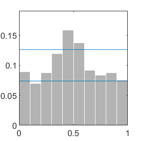
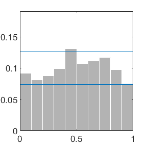
Notes: Teal lines indicate the confidence interval.

Figure 14: Predictive Distributions: Firm-level, 4 Types (Regrouped)

Homog	NP-C/R

Notes: Predictive distributions are regrouped according to predictors. The blue solid / orange dotted / yellow dashed / purple dash-dot lines are the predictive distributions of typical firms a/b/c/d in Figure 4 in the main text, respectively.

Table 10: Two-digit NAICS Codes

Code	Sector
11	Agriculture, Forestry, Fishing and Hunting
21	Mining, Quarrying, and Oil and Gas Extraction
22	Utilities
23	Construction
31-33	Manufacturing
42	Wholesale Trade
44-45	Retail Trade
48-49	Transportation and Warehousing
51	Information
52	Finance and Insurance
53	Real Estate and Rental and Leasing
54	Professional, Scientific, and Technical Services
56	Administrative and Support and Waste Management and Remediation Services
61	Educational Services
62	Health Care and Social Assistance
71	Arts, Entertainment, and Recreation
72	Accommodation and Food Services
81	Other Services (except Public Administration)

Figure 15: Predictive Distributions: Aggregated by Sectors, All Sectors

23	32	33	42
44	45	48	51
52	53	54	56
62	72	81

Notes: Subgraph titles are two-digit NAICS codes. Only sectors with more than 10 firms are shown. The black solid (teal dotted) lines are the predictive distributions via the NP-C/R (Homog).

E.3.2 Discussions

Other Setups.

(1) Choices of variables: In the main text, $y_{it}$ is chosen to be log employment. I adopt log employment instead of the employment growth rate, as the latter significantly reduces the cross-sectional sample size due to the rank requirement. $\text{R\&D}_{it}$ is given by the ratio of a firm’s R&D employment over its total employment considering that R&D employment has more complete observations compared with other innovation intensity gauges.

I have also explored other measures of firm performance (e.g.  log revenue) and innovation activities (e.g.  a binary variable on whether the firm has any R&D expenditure, and a discrete variable on numbers of intellectual properties–patents, copyrights, or trademarks–owned or licensed by the firm). The relative rankings of density forecasts are generally robust across measures.

(2) Model specifications: Following the young firm dynamics literature, for the key variables with potential heterogeneous effects ($w_{i,t-1}$), I also examined the following two setups beyond the R&D setup in the main text:

(a) $w_{i,t-1}=1$, which specifies the baseline model with $\lambda_{i}$ being the individual-specific intercept.

(b) $w_{i,t-1}=\left[1,\;\text{rec}_{t-1}\right]^{\prime}$. $\text{rec}_{t}$ is an aggregate dummy variable indicating the recent recession. It is equal to 1 for 2008 and 2009, and is equal to 0 for other periods.

Results show that for common parameter $\beta$, the posterior means are around $0.4\sim 0.6$ in most cases. For point forecasts, most of the predictors are comparable according to the MSE, with only Flat performing poorly in all three setups. For density forecasts, the overall best across all three setups is Heterosk-NP-C/R in the R&D setup. Comparing across setups, the one with the recession dummy produces the worst density forecasts (and worst point forecasts as well), so the recession dummy with heterogeneous effects does not contribute much to forecasting and may even incur overfitting.

$\beta$ Estimates in the Literature.

Compared to the literature, the closest setup is Zarutskie and Yang (2015) using traditional panel data methods, where the estimated persistence of log employment is 0.824 and 0.816 without firm fixed effects (their Table 2) which is close to Homog, and 0.228 with firm fixed effects estimated via OLS (their Table 4) which is close to Flat.

Conditional Independence between $\lambda_{i}$ and $\sigma_{i}^{2}$.

First, Figure 16 shows the joint distribution of $\hat{\lambda}_{i}$ and $\hat{\sigma}_{i}^{2}$ as well as the joint distribution of $\hat{\sigma}_{i}^{2}$ and the standardized $y_{i0}$, the conditioning variable. There does not seem to be much correlation between $\hat{\lambda}_{i}$ and $\hat{\sigma}_{i}^{2}$ and between $\hat{\sigma}_{i}^{2}$ and $y_{i0}$.

Figure 16: Joint Distributions: $\hat{\lambda}_{i}$, $\hat{\sigma}_{i}^{2}$, and $y_{i0}$

$\hat{\sigma}^{2}_{i}$
	Standardized $y_{i0}$

$\hat{\sigma}^{2}_{i}$
	$\hat{\lambda}_{i1}$

$\hat{\sigma}^{2}_{i}$
	$\hat{\lambda}_{i2}$

Notes: $\lambda_{i1}$ is the heterogeneous intercept, and $\lambda_{i2}$ is the heterogeneous coefficient on R&D.

Second, the correlation matrix together with $p$-values in parentheses (Table 11) delivers a similar message that the uncondtional correlations between $\hat{\lambda}_{i}$ and $\hat{\sigma}_{i}^{2}$ and between $\hat{\sigma}_{i}^{2}$ and $y_{i0}$ are roughly insignificant.

Table 11: Unconditional Correlations: $\hat{\lambda}_{i}$, $\hat{\sigma}_{i}^{2}$, and $y_{i0}$

	$\hat{\lambda}_{i1}$	$\hat{\lambda}_{i2}$	$\hat{\sigma}_{i}^{2}$	$y_{i0}$
$\hat{\lambda}_{i1}$	—
$\hat{\lambda}_{i2}$	0.33 (0.00)	—
$\hat{\sigma}_{i}^{2}$	-0.08 (0.06)	0.02 (0.62)	—
$y_{i0}$	0.70 (0.00)	0.10 (0.02)	-0.10 (0.02)	—

Notes: $\lambda_{i1}$ is the heterogeneous intercept, and $\lambda_{i2}$ is the heterogeneous coefficient on R&D. $p$-values are in parentheses. The entries in bold are significant at the 5% level.

Third, to assess conditional correlation, I considered a regression

$$\hat{\sigma}_{i}^{2}=b_{0}+b_{1}\hat{\lambda}_{i1}+b_{2}\hat{\lambda}_{i2}+b_{3}y_{i0}+\epsilon_{i},$$

where the joint significance of $(b_{1},b_{2})$ could give us an idea regarding the conditional correlation between $\hat{\lambda}_{i}$ and $\hat{\sigma}_{i}^{2}$ conditioning on $y_{i0}$. The estimated $\hat{b}_{1}$ is $-0.02$ with the 95% interval being $[-0.09,0.05]$, and $\hat{b}_{2}$ is $0.06$ with the 95% interval being $[-0.07,0.18]$. Both intervals contain 0. The $p$-value of the $F$-test on $(b_{1},b_{2})$ is 0.92, which is not significant either.

Fourth, to examine conditional independence beyond correlation, I conducted various pairwise conditional independence tests via the R package “bnlearn” (Scutari, 2009). It cannot reject the null hypothesis that $\left.\left(\hat{\lambda}_{i1},\hat{\sigma}_{i}^{2}\right)\right|\left(\hat{\lambda}_{i2},y_{i0}\right)$, $\left.\left(\hat{\lambda}_{i2},\hat{\sigma}_{i}^{2}\right)\right|\left(\hat{\lambda}_{i1},y_{i0}\right)$, $\left.\left(\hat{\lambda}_{i1},\hat{\sigma}_{i}^{2}\right)\right|y_{i0}$, and $\left.\left(\hat{\lambda}_{i2},\hat{\sigma}_{i}^{2}\right)\right|y_{i0}$ are pairwise conditional independent (the corresponding $p$-values are all larger than 0.3). Note that all exercises here are in a “sanity check” manner, and an asymptotic theory of tests is beyond the scope of this paper.

Last but not least, I have also explored the alternative predictor with a joint MGLR_x prior on $h_{i}=\left(\lambda_{i}^{\prime},l_{i}\right)^{\prime}$ mentioned in Appendix B.2. However, the density forecasts significantly deteriorate in both the Monte Carlo simulation and the empirical application (see the first row versus the second row in Table 12). One possible explanation could be that if the true DGP exhibits conditional independence between $\lambda_{i}$ and $\sigma_{i}^{2}$, then although in principle the alternative predictor could approximate the conditional independence structure asymptotically, it could generate overfitting problems and cause inferior out-of-sample density forecasts in finite samples.

Combining the unconditional and conditional evidence based on posterior means of individual heterogeneity as well as the robustness check on density forecast performance, one would be partially confident about the conditional independence assumption in this young firm sample.

Heterogeneous AR(1) Coefficients.

Heterogeneous AR(1) coefficients could be interesting in empirical studies (e.g., Arellano et al. (2017) analyzed earnings and consumption dynamics in a nonlinear panel setup). As a robustness check, I have experimented with a version of heterogeneous persistence $\beta_{i}$ constructed from the best density predictor, NP-C/R, in the empirical application. Unfortunately, its density forecast is significantly worse than the forecast from the specification with homogeneous $\beta$ (see entries (1,1) versus (3,1) in Table 12).

To investigate why this is the case, I turned to the Monte Carlo simulation where the true DGP features homogeneous $\beta$. If we fit a model with heterogeneous persistence, the range of the posterior mean $\hat{\beta}_{i}$ is fairly dispersed, most of $\hat{\beta}_{i}$s appear to be smaller than the true value (this usually happens in time series settings where both the persistence and the initial condition are positive and the sample size is relatively small), and density forecast performance deteriorates in a similar manner as in the empirical application (see entries (1,2) versus (3,2) in Table 12). Therefore, one possible explanation could be that in a relatively small sample, heterogeneous $\beta_{i}$ may tend to fit noise and thus hamper out-of-sample density forecast performance.

Table 12: Density Forecast Evaluation: Robustness Checks

	Empirical	Monte Carlo
NP-C/R	-195***	-1193***
Cond. Correlated $\left(\lambda_{i},\sigma_{i}^{2}\right)$	-506***	-1240***
Heterogeneous $\beta_{i}$	-371***	-1274***

Notes: NP-C/R is the best density predictor in Table 6, which features homogeneous $\beta$ and conditional independence between $\lambda_{i}$ and $\sigma_{i}^{2}$. The tests are conducted with respect to NP-C/R, with significance levels indicated by *: 10%, **: 5%, and ***: 1%. The Monte Carlo part is based on one of the 100 repetitions in the general model with normal $v_{it}$.

References

- Akcigit and Kerr (2018) Akcigit, U. and Kerr, W. R. (2018). Growth through heterogeneous innovations. Journal of Political Economy, 126 (4), 1374–1443.
- Amewou-Atisso et al. (2003) Amewou-Atisso, M., Ghosal, S., Ghosh, J. K. and Ramamoorthi, R. V. (2003). Posterior consistency for semi-parametric regression problems. Bernoulli, 9 (2), 291–312.
- Amisano and Geweke (2017) Amisano, G. and Geweke, J. (2017). Prediction using several macroeconomic models. The Review of Economics and Statistics, 99 (5), 912–925.
- Amisano and Giacomini (2007) — and Giacomini, R. (2007). Comparing density forecasts via weighted likelihood ratio tests. Journal of Business & Economic Statistics, 25 (2), 177–190.
- Antoniak (1974) Antoniak, C. E. (1974). Mixtures of Dirichlet processes with applications to Bayesian nonparametric problems. The Annals of Statistics, pp. 1152–1174.
- Arellano (2003) Arellano, M. (2003). Panel Data Econometrics. Oxford University Press.
- Arellano et al. (2017) —, Blundell, R. and Bonhomme, S. (2017). Earnings and consumption dynamics: a nonlinear panel data framework. Econometrica, 85 (3), 693–734.
- Arellano and Bonhomme (2012) — and Bonhomme, S. (2012). Identifying distributional characteristics in random coefficients panel data models. The Review of Economic Studies, 79 (3), 987–1020.
- Arellano and Bover (1995) — and Bover, O. (1995). Another look at the instrumental variable estimation of error-components models. Journal of Econometrics, 68 (1), 29 – 51.
- Arellano and Honoré (2001) — and Honoré, B. (2001). Panel data models: some recent developments. Handbook of econometrics, 5, 3229–3296.
- Atchadé and Rosenthal (2005) Atchadé, Y. F. and Rosenthal, J. S. (2005). On adaptive Markov chain Monte Carlo algorithms. Bernoulli, 11 (5), 815–828.
- Baltagi (1995) Baltagi, B. (1995). Econometric Analysis of Panel Data. John Wiley & Sons, New York.
- Barron et al. (1999) Barron, A., Schervish, M. J. and Wasserman, L. (1999). The consistency of posterior distributions in nonparametric problems. Ann. Statist., 27 (2), 536–561.
- Basu and Chib (2003) Basu, S. and Chib, S. (2003). Marginal likelihood and Bayes factors for Dirichlet process mixture models. Journal of the American Statistical Association, 98 (461), 224–235.
- Blackwell and Dubins (1962) Blackwell, D. and Dubins, L. (1962). Merging of opinions with increasing information. The Annals of Mathematical Statistics, 33 (3), 882–886.
- Burda and Harding (2013) Burda, M. and Harding, M. (2013). Panel probit with flexible correlated effects: quantifying technology spillovers in the presence of latent heterogeneity. Journal of Applied Econometrics, 28 (6), 956–981.