Joint Embedding of Words and Labels for Text Classification

Abstract

Word embeddings are effective intermediate representations for capturing semantic regularities between words, when learning the representations of text sequences. We propose to view text classification as a label-word joint embedding problem: each label is embedded in the same space with the word vectors. We introduce an attention framework that measures the compatibility of embeddings between text sequences and labels. The attention is learned on a training set of labeled samples to ensure that, given a text sequence, the relevant words are weighted higher than the irrelevant ones. Our method maintains the interpretability of word embeddings, and enjoys a built-in ability to leverage alternative sources of information, in addition to input text sequences. Extensive results on the several large text datasets show that the proposed framework outperforms the state-of-the-art methods by a large margin, in terms of both accuracy and speed.

1 Introduction

Text classification is a fundamental problem in natural language processing (NLP). The task is to annotate a given text sequence with one (or multiple) class label(s) describing its textual content. A key intermediate step is the text representation. Traditional methods represent text with hand-crafted features, such as sparse lexical features (e.g., $n$-grams) Wang and Manning (2012). Recently, neural models have been employed to learn text representations, including convolutional neural networks (CNNs) Kalchbrenner et al. (2014); Zhang et al. (2017b); Shen et al. (2017) and recurrent neural networks (RNNs) based on long short-term memory (LSTM) Hochreiter and Schmidhuber (1997); Wang et al. (2018).

To further increase the representation flexibility of such models, attention mechanisms Bahdanau et al. (2015) have been introduced as an integral part of models employed for text classification Yang et al. (2016). The attention module is trained to capture the dependencies that make significant contributions to the task, regardless of the distance between the elements in the sequence. It can thus provide complementary information to the distance-aware dependencies modeled by RNN/CNN. The increasing representation power of the attention mechanism comes with increased model complexity.

Alternatively, several recent studies show that the success of deep learning on text classification largely depends on the effectiveness of the word embeddings  Joulin et al. (2016); Wieting et al. (2016); Arora et al. (2017); Shen et al. (2018a). Particularly, Shen et al. (2018a) quantitatively show that the word-embeddings-based text classification tasks can have the similar level of difficulty regardless of the employed models, using the concept of intrinsic dimension Li et al. (2018). Thus, simple models are preferred. As the basic building blocks in neural-based NLP, word embeddings capture the similarities/regularities between words Mikolov et al. (2013); Pennington et al. (2014). This idea has been extended to compute embeddings that capture the semantics of word sequences (e.g., phrases, sentences, paragraphs and documents) Le and Mikolov (2014); Kiros et al. (2015). These representations are built upon various types of compositions of word vectors, ranging from simple averaging to sophisticated architectures. Further, they suggest that simple models are efficient and interpretable, and have the potential to outperform sophisticated deep neural models.

It is therefore desirable to leverage the best of both lines of works: learning text representations to capture the dependencies that make significant contributions to the task, while maintaining low computational cost. For the task of text classification, labels play a central role of the final performance. A natural question to ask is how we can directly use label information in constructing the text-sequence representations.

1.1 Our Contribution

Our primary contribution is therefore to propose such a solution by making use of the label embedding framework, and propose the Label-Embedding Attentive Model (LEAM) to improve text classification. While there is an abundant literature in the NLP community on word embeddings (how to describe a word) for text representations, much less work has been devoted in comparison to label embeddings (how to describe a class). The proposed LEAM is implemented by jointly embedding the word and label in the same latent space, and the text representations are constructed directly using the text-label compatibility.

Our label embedding framework has the following salutary properties: $(\textup{\it i})$ Label-attentive text representation is informative for the downstream classification task, as it directly learns from a shared joint space, whereas traditional methods proceed in multiple steps by solving intermediate problems. $(\textup{\it ii})$ The LEAM learning procedure only involves a series of basic algebraic operations, and hence it retains the interpretability of simple models, especially when the label description is available. $(\textup{\it iii})$ Our attention mechanism (derived from the text-label compatibility) has fewer parameters and less computation than related methods, and thus is much cheaper in both training and testing, compared with sophisticated deep attention models. $(\textup{\it iv})$ We perform extensive experiments on several text-classification tasks, demonstrating the effectiveness of our label-embedding attentive model, providing state-of-the-art results on benchmark datasets. $(\textup{\it v})$ We further apply LEAM to predict the medical codes from clinical text. As an interesting by-product, our attentive model can highlight the informative key words for prediction, which in practice can reduce a doctor’s burden on reading clinical notes.

2 Related Work

Label embedding has been shown to be effective in various domains and tasks. In computer vision, there has been a vast amount of research on leveraging label embeddings for image classification (Akata et al., 2016), multimodal learning between images and text (Frome et al., 2013; Kiros et al., 2014), and text recognition in images Rodriguez-Serrano et al. (2013). It is particularly successful on the task of zero-shot learning Palatucci et al. (2009); Yogatama et al. (2015); Ma et al. (2016), where the label correlation captured in the embedding space can improve the prediction when some classes are unseen. In NLP, labels embedding for text classification has been studied in the context of heterogeneous networks in (Tang et al., 2015) and multitask learning in (Zhang et al., 2017a), respectively. To the authors’ knowledge, there is little research on investigating the effectiveness of label embeddings to design efficient attention models, and how to joint embedding of words and labels to make full use of label information for text classification has not been studied previously, representing a contribution of this paper.

For text representation, the currently best-performing models usually consist of an encoder and a decoder connected through an attention mechanism Vaswani et al. (2017); Bahdanau et al. (2015), with successful applications to sentiment classification Zhou et al. (2016), sentence pair modeling Yin et al. (2016) and sentence summarization Rush et al. (2015). Based on this success, more advanced attention models have been developed, including hierarchical attention networks Yang et al. (2016), attention over attention Cui et al. (2016), and multi-step attention Gehring et al. (2017). The idea of attention is motivated by the observation that different words in the same context are differentially informative, and the same word may be differentially important in a different context. The realization of “context” varies in different applications and model architectures. Typically, the context is chosen as the target task, and the attention is computed over the hidden layers of a CNN/RNN. Our attention model is directly built in the joint embedding space of words and labels, and the context is specified by the label embedding.

Several recent works Vaswani et al. (2017); Shen et al. (2018b, c) have demonstrated that simple attention architectures can alone achieve state-of-the-art performance with less computational time, dispensing with recurrence and convolutions entirely. Our work is in the same direction, sharing the similar spirit of retaining model simplicity and interpretability. The major difference is that the aforementioned work focused on self attention, which applies attention to each pair of word tokens from the text sequences. In this paper, we investigate the attention between words and labels, which is more directly related to the target task. Furthermore, the proposed LEAM has much less model parameters.

3 Preliminaries

Throughout this paper, we denote vectors as bold, lower-case letters, and matrices as bold, upper-case letters. We use $\oslash$ for element-wise division when applied to vectors or matrices. We use $\circ$ for function composition, and $\Delta^{p}$ for the set of one hot vectors in dimension $p$.

Given a training set $\mathcal{S}=\{({{\bf X}}_{n},\bm{y}_{n})\}_{n=1}^{N}$ of pair-wise data, where ${{\bf X}}\in\mathcal{X}$ is the text sequence, and $\bm{y}\in\mathcal{Y}$ is its corresponding label. Specifically, $\bm{y}$ is a one hot vector in single-label problem and a binary vector in multi-label problem, as defined later in Section 4.1. Our goal for text classification is to learn a function $f:\mathcal{X}\mapsto\mathcal{Y}$ by minimizing an empirical risk of the form:

$$\min_{f\in\mathcal{F}}\frac{1}{N}\sum_{n=1}^{N}\delta(\bm{y}_{n},f({{\bf X}}_{n}))\vspace{-2mm}\vspace{0mm}$$ (1)

where $\delta:\mathcal{Y}\times\mathcal{Y}\mapsto\mathbb{R}$ measures the loss incurred from predicting $f({{\bf X}})$ when the true label is $\bm{y}$, where $f$ belongs to the functional space $\mathcal{F}$. In the evaluation stage, we shall use the $0/1$ loss as a target loss: $\delta(\bm{y},\bm{z})=0$ if $\bm{y}=\bm{z}$, and $1$ otherwise. In the training stage, we consider surrogate losses commonly used for structured prediction in different problem setups (see Section 4.1 for details on the surrogate losses used in this paper).

More specifically, an input sequence ${{\bf X}}$ of length $L$ is composed of word tokens: ${{\bf X}}=\{\bm{x}_{1},\cdots,\bm{x}_{L}\}$. Each token $\bm{x}_{l}$ is a one hot vector in the space $\Delta^{D}$, where $D$ is the dictionary size. Performing learning in $\Delta^{D}$ is computationally expensive and difficult. An elegant framework in NLP, initially proposed in Mikolov et al. (2013); Le and Mikolov (2014); Pennington et al. (2014); Kiros et al. (2015), allows to concisely perform learning by mapping the words into an embedding space. The framework relies on so called word embedding: $\Delta^{D}\mapsto\mathbb{R}^{P}$, where $P$ is the dimensionality of the embedding space. Therefore, the text sequence ${{\bf X}}$ is represented via the respective word embedding for each token: ${{\bf V}}=\{\bm{v}_{1},\cdots,\bm{v}_{L}\}$, where $\bm{v}_{l}\in\mathbb{R}^{P}$. A typical text classification method proceeds in three steps, end-to-end, by considering a function decomposition $f=f_{0}\circ f_{1}\circ f_{2}$ as shown in Figure 1(a):

• $f_{0}:{{\bf X}}\mapsto{{\bf V}}$, the text sequence is represented as its word-embedding form ${{\bf V}}$, which is a matrix of $P\times L$.

• $f_{1}:{{\bf V}}\mapsto\bm{z}$, a compositional function $f_{1}$ aggregates word embeddings into a fixed-length vector representation $\bm{z}$.

• $f_{2}:\bm{z}\mapsto\bm{y}$, a classifier $f_{2}$ annotates the text representation $\bm{z}$ with a label.

A vast amount of work has been devoted to devising the proper functions $f_{0}$ and $f_{1}$, i.e., how to represent a word or a word sequence, respectively. The success of NLP largely depends on the effectiveness of word embeddings in $f_{0}$ Bengio et al. (2003); Collobert and Weston (2008); Mikolov et al. (2013); Pennington et al. (2014). They are often pre-trained offline on large corpus, then refined jointly via $f_{1}$ and $f_{2}$ for task-specific representations. Furthermore, the design of $f_{1}$ can be broadly cast into two categories. The popular deep learning models consider the mapping as a “black box,” and have employed sophisticated CNN/RNN architectures to achieve state-of-the-art performance Zhang et al. (2015); Yang et al. (2016). On the contrary, recent studies show that simple manipulation of the word embeddings, e.g., mean or max-pooling, can also provide surprisingly excellent performance Joulin et al. (2016); Wieting et al. (2016); Arora et al. (2017); Shen et al. (2018a). Nevertheless, these methods only leverage the information from the input text sequence.

4 Label-Embedding Attentive Model

(a) Traditional method

(b) Proposed joint embedding method

Figure 1: Illustration of different schemes for document representations $\bm{z}$. (a) Much work in NLP has been devoted to directly aggregating word embedding ${{\bf V}}$ for $\bm{z}$. (b) We focus on learning label embedding ${\bf C}$ (how to embed class labels in a Euclidean space), and leveraging the “compatibility” ${\bf G}$ between embedded words and labels to derive the attention score ${\bm{\beta}}$ for improved $\bm{z}$. Note that $\otimes$ denotes the cosine similarity between ${\bf C}$ and ${{\bf V}}$. In this figure, there are K=2 classes.

4.1 Model

By examining the three steps in the traditional pipeline of text classification, we note that the use of label information only occurs in the last step, when learning $f_{2}$, and its impact on learning the representations of words in $f_{0}$ or word sequences in $f_{1}$ is ignored or indirect. Hence, we propose a new pipeline by incorporating label information in every step, as shown in Figure 1(b):

• $f_{0}$: Besides embedding words, we also embed all the labels in the same space, which act as the “anchor points” of the classes to influence the refinement of word embeddings.

• $f_{1}$: The compositional function aggregates word embeddings into $\bm{z}$, weighted by the compatibility between labels and words.

• $f_{2}$: The learning of $f_{2}$ remains the same, as it directly interacts with labels.

Under the proposed label embedding framework, we specifically describe a label-embedding attentive model.

Joint Embeddings of Words and Labels

We propose to embed both the words and the labels into a joint space i.e., $\Delta^{D}\mapsto\mathbb{R}^{P}$ and $\mathcal{Y}\mapsto\mathbb{R}^{P}$. The label embeddings are ${\bf C}=[{\bm{c}}_{1},\cdots,{\bm{c}}_{K}]$, where $K$ is the number of classes.

A simple way to measure the compatibility of label-word pairs is via the cosine similarity

$${\bf G}=({\bf C}^{\top}{{\bf V}})\oslash\hat{{\bf G}},\vspace{0mm}$$ (2)

where $\hat{{\bf G}}$ is the normalization matrix of size $K\times L$, with each element obtained as the multiplication of $\ell_{2}$ norms of the $c$-th label embedding and $l$-th word embedding: $\hat{g}_{kl}=\|{\bm{c}}_{k}\|\|\bm{v}_{l}\|$.

To further capture the relative spatial information among consecutive words (i.e., phrases) and introduce non-linearity in the compatibility measure, we consider a generalization of (2). Specifically, for a text phase of length $2r+1$ centered at $l$, the local matrix block ${\bf G}_{l-r:l+r}$ in ${\bf G}$ measures the label-to-token compatibility for the “label-phrase” pairs. To learn a higher-level compatibility stigmatization $\bm{u}_{l}$ between the $l$-th phrase and all labels, we have:

$${\bm{u}_{l}=\mbox{ReLU}({\bf G}_{l-r:l+r}{{\bf W}}_{1}+{\bm{b}}_{1}),}\vspace{0mm}$$ (3)

where ${{\bf W}}_{1}\in\mathbb{R}^{2r+1}$ and ${\bm{b}}_{1}\in\mathbb{R}^{K}$ are parameters to be learned, and $\bm{u}_{l}\in\mathbb{R}^{K}$. The largest compatibility value of the $l$-th phrase wrt the labels is collected:

$${m_{l}=\mbox{max-pooling}(\bm{u}_{l}).}\vspace{0mm}$$ (4)

Together, ${\bm{m}}$ is a vector of length $L$. The compatibility/attention score for the entire text sequence is:

$${{\bm{\beta}}=\mbox{SoftMax}({\bm{m}}),}\vspace{0mm}$$ (5)

where the $l$-th element of SoftMax is $\beta_{l}=\frac{\exp(m_{l})}{\sum_{l^{\prime}=1}^{L}\exp(m_{l^{\prime}})}$.

The text sequence representation can be simply obtained via averaging the word embeddings, weighted by label-based attention score:

$${\bm{z}=\sum_{l}\beta_{l}\bm{v}_{l}.}\vspace{0mm}$$ (6)

Relation to Predictive Text Embeddings

Predictive Text Embeddings (PTE) (Tang et al., 2015) is the first method to leverage label embeddings to improve the learned word embeddings. We discuss three major differences between PTE and our LEAM: $(\textup{\it i})$ The general settings are different. PTE casts the text representation through heterogeneous networks, while we consider text representation through an attention model. $(\textup{\it ii})$ In PTE, the text representation $\bm{z}$ is the averaging of word embeddings. In LEAM, $\bm{z}$ is weighted averaging of word embeddings through the proposed label-attentive score in (6). $(\textup{\it iii})$ PTE only considers the linear interaction between individual words and labels. LEAM greatly improves the performance by considering nonlinear interaction between phrase and labels. Specifically, we note that the text embedding in PTE is similar with a very special case of LEAM, when our window size $r=1$ and attention score ${\bm{\beta}}$ is uniform. As shown later in Figure 2(c) of the experimental results, LEAM can be significantly better than the PTE variant.

Training Objective

The proposed joint embedding framework is applicable to various text classification tasks. We consider two setups in this paper. For a learned text sequence representation $\bm{z}=f_{1}\circ f_{0}({{\bf X}})$, we jointly optimize $f=f_{0}\circ f_{1}\circ f_{2}$ over $\mathcal{F}$, where $f_{2}$ is defined according to the specific tasks:

• Single-label problem: categorizes each text instance to precisely one of $K$ classes, $\bm{y}\in\Delta^{K}$

  $$\min_{f\in\mathcal{F}}\frac{1}{N}\sum_{n=1}^{N}\mbox{CE}(\bm{y}_{n},f_{2}(\bm{z}_{n})),\vspace{0mm}$$ (7)

  where $\mbox{CE}(\cdot,\cdot)$ is the cross entropy between two probability vectors, and $f_{2}(\bm{z}_{n})=\mbox{SoftMax }(\bm{z}_{n}^{\prime})$, with $\bm{z}_{n}^{\prime}={{\bf W}}_{2}\bm{z}_{n}+{\bm{b}}_{2}$ and ${{\bf W}}_{2}\in\mathbb{R}^{K\times P},{\bm{b}}_{2}\in\mathbb{R}^{K}$ are trainable parameters.

• Multi-label problem: categorizes each text instance to a set of $K$ target labels $\{\bm{y}_{k}\in\Delta^{2}|k=1,\cdots,K\}$; there is no constraint on how many of the classes the instance can be assigned to, and

  $$\min_{f\in\mathcal{F}}\frac{1}{NK}\sum_{n=1}^{N}\sum_{k=1}^{K}\mbox{CE}(\bm{y}_{nk},f_{2}(\bm{z}_{nk}),\vspace{0mm}$$ (8)

  where $f_{2}(\bm{z}_{nk})=\frac{1}{1+\exp(\bm{z}_{nk}^{\prime})}$, and $\bm{z}_{nk}^{\prime}$ is the $k$th column of $\bm{z}_{n}^{\prime}$.

To summarize, the model parameters $\bm{\theta}=\{{{\bf V}},{\bf C},{{\bf W}}_{1},{\bm{b}}_{1},{{\bf W}}_{2},{\bm{b}}_{2}\}$. They are trained end-to-end during learning. $\{{{\bf W}}_{1},{\bm{b}}_{1}\}$ and $\{{{\bf W}}_{2},{\bm{b}}_{2}\}$ are weights in $f_{1}$ and $f_{2}$, respectively, which are treated as standard neural networks. For the joint embeddings $\{{{\bf V}},{\bf C}\}$ in $f_{0}$, the pre-trained word embeddings are used as initialization if available.

4.2 Learning & Testing with LEAM

Learning and Regularization

The quality of the jointly learned embeddings are key to the model performance and interpretability. Ideally, we hope that each label embedding acts as the “anchor” points for each classes: closer to the word/sequence representations that are in the same classes, while farther from those in different classes. To best achieve this property, we consider to regularize the learned label embeddings ${\bm{c}}_{k}$ to be on its corresponding manifold. This is imposed by the fact ${\bm{c}}_{k}$ should be easily classified as the correct label $\bm{y}_{k}$:

$$\min_{f\in\mathcal{F}}\frac{1}{K}\sum_{n=1}^{K}\mbox{CE}(\bm{y}_{k},f_{2}({\bm{c}}_{k})),\vspace{0mm}$$ (9)

where $f_{2}$ is specficied according to the problem in either (7) or (8). This regularization is used as a penalty in the main training objective in (7) or (8), and the default weighting hyperparameter is set as 1. It will lead to meaningful interpretability of learned label embeddings as shown in the experiments.

Interestingly in text classification, the class itself is often described as a set of $E$ words $\{{\bm{e}}_{i},i=1,\cdots,E\}$. These words are considered as the most representative description of each class, and highly distinguishing between different classes. For example, the $\mathtt{Yahoo!~{}Answers~{}Topic}$ dataset Zhang et al. (2015) contains ten classes, most of which have two words to precisely describe its class-specific features, such as “Computers & Internet”, “Business & Finance” as well as “Politics & Government” etc. We consider to use each label’s corresponding pre-trained word embeddings as the initialization of the label embeddings. For the datasets without representative class descriptions, one may initialize the label embeddings as random samples drawn from a standard Gaussian distribution.

Testing

Both the learned word and label embeddings are available in the testing stage. We clarify that the label embeddings ${\bf C}$ of all class candidates $\mathcal{Y}$ are considered as the input in the testing stage; one should distinguish this from the use of groundtruth label $\bm{y}$ in prediction. For a text sequence ${{\bf X}}$, one may feed it through the proposed pipeline for prediction: $(\textup{\it i})$ $f_{1}$: harvesting the word embeddings ${{\bf V}}$, $(\textup{\it ii})$ $f_{2}$: ${{\bf V}}$ interacts with ${\bf C}$ to obtain ${\bf G}$, pooled as ${\bm{\beta}}$, which further attends ${{\bf V}}$ to derive $\bm{z}$, and $(\textup{\it iii})$ $f_{3}$: assigning labels based on the tasks. To speed up testing, one may store ${\bf G}$ offline, and avoid its online computational cost.

4.3 Model Complexity

We compare CNN, LSTM, Simple Word Embeddings-based Models (SWEM) Shen et al. (2018a) and our LEAM wrt the parameters and computational speed. For the CNN, we assume the same size $m$ for all filters. Specifically, $h$ represents the dimension of the hidden units in the LSTM or the number of filters in the CNN; $R$ denotes the number of blocks in the Bi-BloSAN; $P$ denotes the final sequence representation dimension. Similar to Vaswani et al. (2017); Shen et al. (2018a), we examine the number of compositional parameters, computational complexity and sequential steps of the four methods. As shown in Table LABEL:tab:archit_compare, both the CNN and LSTM have a large number of compositional parameters. Since $K\ll m,h$, the number of parameters in our models is much smaller than for the CNN and LSTM models. For the computational complexity, our model is almost same order as the most simple SWEM model, and is smaller than the CNN or LSTM by a factor of $mh/K$ or $h/K$.

5 Experimental Results

Setup

We use 300-dimensional GloVe word embeddings Pennington et al. (2014) as initialization for word embeddings and label embeddings in our model. Out-Of-Vocabulary (OOV) words are initialized from a uniform distribution with range $[-0.01,0.01]$. The final classifier is implemented as an MLP layer followed by a sigmoid or softmax function depending on specific task. We train our model’s parameters with the Adam Optimizer (Kingma and Ba, 2014), with an initial learning rate of $0.001$, and a minibatch size of 100. Dropout regularization (Srivastava et al., 2014) is employed on the final MLP layer, with dropout rate $0.5$. The model is implemented using Tensorflow and is trained on GPU Titan X.

The code to reproduce the experimental results is at  https://github.com/guoyinwang/LEAM

5.1 Classification on Benchmark Datasets

We test our model on the same five standard benchmark datasets as in (Zhang et al., 2015). The summary statistics of the data are shown in Table LABEL:tab:datasets, with content specified below:

• $\mathtt{AGNews}$: Topic classification over four categories of Internet news articles (Del Corso et al., 2005) composed of titles plus description classified into: World, Entertainment, Sports and Business.

• $\mathtt{Yelp~{}~{}Review~{}~{}Full}$: The dataset is obtained from the Yelp Dataset Challenge in 2015, the task is sentiment classification of polarity star labels ranging from 1 to 5.

• $\mathtt{Yelp~{}~{}Review~{}~{}Polarity}$: The same set of text reviews from Yelp Dataset Challenge in 2015, except that a coarser sentiment definition is considered: 1 and 2 are negative, and 4 and 5 as positive.

• $\mathtt{DBPedia}$: Ontology classification over fourteen non-overlapping classes picked from DBpedia 2014 (Wikipedia).

• $\mathtt{Yahoo!~{}~{}Answers~{}~{}Topic}$: Topic classification over ten largest main categories from Yahoo! Answers Comprehensive Questions and Answers version 1.0, including question title, question content and best answer.

Model	Yahoo	DBPedia	AGNews	Yelp P.	Yelp F.
Bag-of-words (Zhang et al., 2015)	68.90	96.60	88.80	92.20	58.00
Small word CNN (Zhang et al., 2015)	69.98	98.15	89.13	94.46	58.59
Large word CNN (Zhang et al., 2015)	70.94	98.28	91.45	95.11	59.48
LSTM (Zhang et al., 2015)	70.84	98.55	86.06	94.74	58.17
SA-LSTM (word-level) (Dai and Le, 2015)	-	98.60	-	-	-
Deep CNN (29 layer) (Conneau et al., 2017)	73.43	98.71	91.27	95.72	64.26
SWEM (Shen et al., 2018a)	73.53	98.42	92.24	93.76	61.11
fastText (Joulin et al., 2016)	72.30	98.60	92.50	95.70	63.90
HAN (Yang et al., 2016)	75.80	-	-	-	-
Bi-BloSAN⋄ (Shen et al., 2018c)	76.28	98.77	93.32	94.56	62.13
LEAM	77.42	99.02	92.45	95.31	64.09
LEAM (linear)	75.22	98.32	91.75	93.43	61.03

Table 3: Test Accuracy on document classification tasks, in percentage. ^⋄ We ran Bi-BloSAN using the authors’ implementation; all other results are directly cited from the respective papers.

We compare with a variety of methods, including $(\textup{\it i})$ the bag-of-words in (Zhang et al., 2015); $(\textup{\it ii})$ sophisticated deep CNN/RNN models: large/small word CNN, LSTM reported in (Zhang et al., 2015; Dai and Le, 2015) and deep CNN (29 layer) (Conneau et al., 2017); $(\textup{\it iii})$ simple compositional methods: fastText (Joulin et al., 2016) and simple word embedding models (SWEM) (Shen et al., 2018a); $(\textup{\it iv})$ deep attention models: hierarchical attention network (HAN) (Yang et al., 2016); $(\textup{\it v})$ simple attention models: bi-directional block self-attention network (Bi-BloSAN) (Shen et al., 2018c). The results are shown in Table 3.

Testing accuracy

Simple compositional methods indeed achieve comparable performance as the sophisticated deep CNN/RNN models. On the other hand, deep hierarchical attention model can improve the pure CNN/RNN models. The recently proposed self-attention network generally yield higher accuracy than previous methods. All approaches are better than traditional bag-of-words method. Our proposed LEAM outperforms the state-of-the-art methods on two largest datasets, i.e., Yahoo and DBPedia. On other datasets, LEAM ranks the 2nd or 3rd best, which are similar to top 1 method in term of the accuracy. This is probably due to two reasons: $(\textup{\it i})$ the number of classes on these datasets is smaller, and $(\textup{\it ii})$ there is no explicit corresponding word embedding available for the label embedding initialization during learning. The potential of label embedding may not be fully exploited. As the ablation study, we replace the nonlinear compatibility (3) to the linear one in (2) . The degraded performance demonstrates the necessity of spatial dependency and nonlinearity in constructing the attentions.

Nevertheless, we argue LEAM is favorable for text classification, by comparing the model size and time cost Table LABEL:tab:model_complexity, as well as convergence speed in Figure 2(a). The time cost is reported as the wall-clock time for 1000 iterations. LEAM maintains the simplicity and low cost of SWEM, compared with other models. LEAM uses much less model parameters, and converges significantly faster than Bi-BloSAN. We also compare the performance when only a partial dataset is labeled, the results are shown in Figure 2(b). LEAM consistently outperforms other methods with different proportion of labeled data.

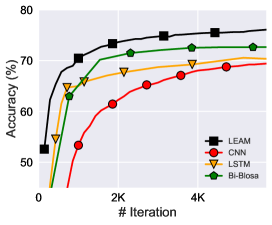
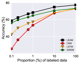
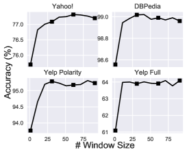
(a) Convergence speed	(b) Partially labeled data	(c) Effects of window size

Figure 2: Comprehensive study of LEAM, including convergence speed, performance vs proportion of labeled data, and impact of hyper-parameter

Hyper-parameter

Our method has an additional hyperparameter, the window size $r$ to define the length of “phase” to construct the attention. Larger $r$ captures long term dependency, while smaller $r$ enforces the local dependency. We study its impact in Figure 2(c). The topic classification tasks generally requires a larger $r$, while sentiment classification tasks allows relatively smaller $r$. One may safely choose $r$ around $50$ if not finetuning. We report the optimal results in Table 3.

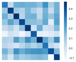
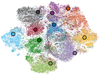
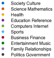
(a) Cosine similarity matrix	(b) t-SNE plot of joint embeddings

Figure 3: Correlation between the learned text sequence representation $\bm{z}$ and label embedding ${{\bf V}}$. (a) Cosine similarity matrix between averaged $\bar{\bm{z}}$ per class and label embedding ${{\bf V}}$, and (b) t-SNE plot of joint embedding of text $\bm{z}$ and labels ${{\bf V}}$.

5.2 Representational Ability

Label embeddings are highly meaningful

To provide insight into the meaningfulness of the learned representations, in Figure 3 we visualize the correlation between label embeddings and document embeddings based on the Yahoo dateset. First, we compute the averaged document embeddings per class: $\bar{\bm{z}}_{k}=\frac{1}{|\mathcal{S}_{k}|}\sum_{i\in\mathcal{S}_{k}}\bm{z}_{i}$, where $\mathcal{S}_{k}$ is the set of sample indices belonging to class $k$. Intuitively, $\bar{\bm{z}}_{k}$ represents the center of embedded text manifold for class $k$. Ideally, the perfect label embedding ${\bm{c}}_{k}$ should be the representative anchor point for class $k$. We compute the cosine similarity between $\bar{\bm{z}_{k}}$ and ${\bm{c}}_{k}$ across all the classes, shown in Figure 3(a). The rows are averaged per-class document embeddings, while columns are label embeddings. Therefore, the on-diagonal elements measure how representative the learned label embeddings are to describe its own classes, while off-diagonal elements reflect how distinctive the label embeddings are to be separated from other classes. The high on-diagonal elements and low off-diagonal elements in Figure 3(a) indicate the superb ability of the label representations learned from LEAM.

Further, since both the document and label embeddings live in the same high-dimensional space, we use t-SNE (Maaten and Hinton, 2008) to visualize them on a 2D map in Figure 3(b). Each color represents a different class, the point clouds are document embeddings, and the label embeddings are the large dots with black circles. As can be seen, each label embedding falls into the internal region of the respective manifold, which again demonstrate the strong representative power of label embeddings.

Interpretability of attention

Our attention score ${\bm{\beta}}$ can be used to highlight the most informative words wrt the downstream prediction task. We visualize two examples in Figure 4(a) for the Yahoo dataset. The darker yellow means more important words. The 1st text sequence is on the topic of “Sports”, and the 2nd text sequence is “Entertainment”. The attention score can correctly detect the key words with proper scores.

5.3 Applications to Clinical Text

To demonstrate the practical value of label embeddings, we apply LEAM for a real health care scenario: medical code prediction on the Electronic Health Records dataset. A given patient may have multiple diagnoses, and thus multi-label learning is required.

Specifically, we consider an open-access dataset, $\mathtt{MIMIC}$-$\mathtt{III}$ Johnson et al. (2016), which contains text and structured records from a hospital intensive care unit. Each record includes a variety of narrative notes describing a patient’s stay, including diagnoses and procedures. They are accompanied by a set of metadata codes from the International Classification of Diseases (ICD), which present a standardized way of indicating diagnoses/procedures. To compare with previous work, we follow Shi et al. (2017); Mullenbach et al. (2018), and preprocess a dataset consisting of the most common 50 labels. It results in 8,067 documents for training, 1,574 for validation, and 1,730 for testing.

Results

We compare against the three baselines: a logistic regression model with bag-of-words, a bidirectional gated recurrent unit (Bi-GRU) and a single-layer 1D convolutional network Kim (2014). We also compare with three recent methods for multi-label classification of clinical text, including Condensed Memory Networks (C-MemNN) Prakash et al. (2017), Attentive LSTM Shi et al. (2017) and Convolutional Attention (CAML) Mullenbach et al. (2018).

To quantify the prediction performance, we follow Mullenbach et al. (2018) to consider the micro-averaged and macro-averaged F1 and area under the ROC curve (AUC), as well as the precision at $n$ (P@$n$). Micro-averaged values are calculated by treating each (text, code) pair as a separate prediction. Macro-averaged values are calculated by averaging metrics computed per-label. P@$n$ is the fraction of the $n$ highestscored labels that are present in the ground truth.

The results are shown in Table LABEL:tab:multilabel-results. LEAM provides the best AUC score, and better F1 and P@5 values than all methods except CNN. CNN consistently outperforms the basic Bi-GRU architecture, and the logistic regression baseline performs worse than all deep learning architectures.

We emphasize that the learned attention can be very useful to reduce a doctor’s reading burden. As shown in Figure 4(b), the health related words are highlighted.

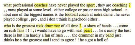
(a) Yahoo dataset

(b) Clinical text

Figure 4: Visualization of learned attention ${\bm{\beta}}$.

6 Conclusions

In this work, we first investigate label embeddings for text representations, and propose the label-embedding attentive models. It embeds the words and labels in the same joint space, and measures the compatibility of word-label pairs to attend the document representations. The learning framework is tested on several large standard datasets and a real clinical text application. Compared with the previous methods, our LEAM algorithm requires much lower computational cost, and achieves better if not comparable performance relative to the state-of-the-art. The learned attention is highly interpretable: highlighting the most informative words in the text sequence for the downstream classification task.

Acknowledgments

This research was supported by DARPA, DOE, NIH, ONR and NSF.

References

- Akata et al. (2016) Zeynep Akata, Florent Perronnin, Zaid Harchaoui, and Cordelia Schmid. 2016. Label-embedding for image classification. IEEE transactions on pattern analysis and machine intelligence.
- Arora et al. (2017) Sanjeev Arora, Yingyu Liang, and Tengyu Ma. 2017. A simple but tough-to-beat baseline for sentence embeddings. ICLR.
- Bahdanau et al. (2015) Dzmitry Bahdanau, Kyunghyun Cho, and Yoshua Bengio. 2015. Neural machine translation by jointly learning to align and translate. ICLR.
- Bengio et al. (2003) Yoshua Bengio, Réjean Ducharme, Pascal Vincent, and Christian Jauvin. 2003. A neural probabilistic language model. Journal of machine learning research.
- Collobert and Weston (2008) Ronan Collobert and Jason Weston. 2008. A unified architecture for natural language processing: Deep neural networks with multitask learning. In Proceedings of the 25th international conference on Machine learning.
- Conneau et al. (2017) Alexis Conneau, Holger Schwenk, Loïc Barrault, and Yann Lecun. 2017. Very deep convolutional networks for text classification. In Proceedings of the 15th Conference of the European Chapter of the Association for Computational Linguistics: Volume 1, Long Papers, volume 1, pages 1107–1116.
- Cui et al. (2016) Yiming Cui, Zhipeng Chen, Si Wei, Shijin Wang, Ting Liu, and Guoping Hu. 2016. Attention-over-attention neural networks for reading comprehension. arXiv preprint arXiv:1607.04423.
- Dai and Le (2015) Andrew M Dai and Quoc V Le. 2015. Semi-supervised sequence learning. In Advances in Neural Information Processing Systems, pages 3079–3087.
- Del Corso et al. (2005) Gianna M Del Corso, Antonio Gulli, and Francesco Romani. 2005. Ranking a stream of news. In Proceedings of the 14th international conference on World Wide Web. ACM.
- Frome et al. (2013) Andrea Frome, Greg S Corrado, Jon Shlens, Samy Bengio, Jeff Dean, Tomas Mikolov, et al. 2013. Devise: A deep visual-semantic embedding model. In NIPS.
- Gehring et al. (2017) Jonas Gehring, Michael Auli, David Grangier, Denis Yarats, and Yann N Dauphin. 2017. Convolutional sequence to sequence learning. arXiv preprint arXiv:1705.03122.
- Hochreiter and Schmidhuber (1997) Sepp Hochreiter and Jürgen Schmidhuber. 1997. Long short-term memory. Neural computation.
- Johnson et al. (2016) Alistair EW Johnson, Tom J Pollard, Lu Shen, H Lehman Li-wei, Mengling Feng, Mohammad Ghassemi, Benjamin Moody, Peter Szolovits, Leo Anthony Celi, and Roger G Mark. 2016. Mimic-iii, a freely accessible critical care database. Scientific data.
- Joulin et al. (2016) Armand Joulin, Edouard Grave, Piotr Bojanowski, and Tomas Mikolov. 2016. Bag of tricks for efficient text classification. EACL.
- Kalchbrenner et al. (2014) Nal Kalchbrenner, Edward Grefenstette, and Phil Blunsom. 2014. A convolutional neural network for modelling sentences. ACL.
- Kim (2014) Yoon Kim. 2014. Convolutional neural networks for sentence classification. arXiv preprint arXiv:1408.5882.
- Kingma and Ba (2014) Diederik P Kingma and Jimmy Ba. 2014. Adam: A method for stochastic optimization. arXiv preprint arXiv:1412.6980.
- Kiros et al. (2014) Ryan Kiros, Ruslan Salakhutdinov, and Richard S Zemel. 2014. Unifying visual-semantic embeddings with multimodal neural language models. NIPS 2014 deep learning workshop.
- Kiros et al. (2015) Ryan Kiros, Yukun Zhu, Ruslan R Salakhutdinov, Richard Zemel, Raquel Urtasun, Antonio Torralba, and Sanja Fidler. 2015. Skip-thought vectors. In Advances in neural information processing systems.
- Le and Mikolov (2014) Quoc Le and Tomas Mikolov. 2014. Distributed representations of sentences and documents. In International Conference on Machine Learning, pages 1188–1196.
- Li et al. (2018) Chunyuan Li, Heerad Farkhoor, Rosanne Liu, and Jason Yosinski. 2018. Measuring the intrinsic dimension of objective landscapes. In International Conference on Learning Representations.
- Ma et al. (2016) Yukun Ma, Erik Cambria, and Sa Gao. 2016. Label embedding for zero-shot fine-grained named entity typing. In COLING.
- Maaten and Hinton (2008) Laurens van der Maaten and Geoffrey Hinton. 2008. Visualizing data using t-sne. Journal of machine learning research.
- Mikolov et al. (2013) Tomas Mikolov, Ilya Sutskever, Kai Chen, Greg S Corrado, and Jeff Dean. 2013. Distributed representations of words and phrases and their compositionality. In Advances in neural information processing systems, pages 3111–3119.
- Mullenbach et al. (2018) James Mullenbach, Sarah Wiegreffe, Jon Duke, Jimeng Sun, and Jacob Eisenstein. 2018. Explainable prediction of medical codes from clinical text. arXiv preprint arXiv:1802.05695.
- Palatucci et al. (2009) Mark Palatucci, Dean Pomerleau, Geoffrey E Hinton, and Tom M Mitchell. 2009. Zero-shot learning with semantic output codes. In NIPS.
- Pennington et al. (2014) Jeffrey Pennington, Richard Socher, and Christopher Manning. 2014. Glove: Global vectors for word representation. In Proceedings of the 2014 conference on empirical methods in natural language processing (EMNLP), pages 1532–1543.
- Prakash et al. (2017) Aaditya Prakash, Siyuan Zhao, Sadid A Hasan, Vivek V Datla, Kathy Lee, Ashequl Qadir, Joey Liu, and Oladimeji Farri. 2017. Condensed memory networks for clinical diagnostic inferencing. In AAAI.
- Rodriguez-Serrano et al. (2013) Jose A Rodriguez-Serrano, Florent Perronnin, and France Meylan. 2013. Label embedding for text recognition. In Proceedings of the British Machine Vision Conference.
- Rush et al. (2015) Alexander M Rush, Sumit Chopra, and Jason Weston. 2015. A neural attention model for abstractive sentence summarization. arXiv preprint arXiv:1509.00685.
- Shen et al. (2018a) Dinghan Shen, Guoyin Wang, Wenlin Wang, Martin Renqiang Min, Qinliang Su, Yizhe Zhang, Chunyuan Li, Ricardo Henao, and Lawrence Carin. 2018a. Baseline needs more love: On simple word-embedding-based models and associated pooling mechanisms. In ACL.
- Shen et al. (2017) Dinghan Shen, Yizhe Zhang, Ricardo Henao, Qinliang Su, and Lawrence Carin. 2017. Deconvolutional latent-variable model for text sequence matching. AAAI.
- Shen et al. (2018b) Tao Shen, Tianyi Zhou, Guodong Long, Jing Jiang, Shirui Pan, and Chengqi Zhang. 2018b. Disan: Directional self-attention network for rnn/cnn-free language understanding. AAAI.
- Shen et al. (2018c) Tao Shen, Tianyi Zhou, Guodong Long, Jing Jiang, and Chengqi Zhang. 2018c. Bi-directional block self-attention for fast and memory-efficient sequence modeling. ICLR.
- Shi et al. (2017) Haoran Shi, Pengtao Xie, Zhiting Hu, Ming Zhang, and Eric P Xing. 2017. Towards automated icd coding using deep learning. arXiv preprint arXiv:1711.04075.
- Srivastava et al. (2014) Nitish Srivastava, Geoffrey Hinton, Alex Krizhevsky, Ilya Sutskever, and Ruslan Salakhutdinov. 2014. Dropout: A simple way to prevent neural networks from overfitting. The Journal of Machine Learning Research.
- Tang et al. (2015) Jian Tang, Meng Qu, and Qiaozhu Mei. 2015. Pte: Predictive text embedding through large-scale heterogeneous text networks. In Proceedings of the 21th ACM SIGKDD International Conference on Knowledge Discovery and Data Mining, pages 1165–1174. ACM.
- Vaswani et al. (2017) Ashish Vaswani, Noam Shazeer, Niki Parmar, Jakob Uszkoreit, Llion Jones, Aidan N Gomez, Łukasz Kaiser, and Illia Polosukhin. 2017. Attention is all you need. In Advances in Neural Information Processing Systems, pages 6000–6010.
- Wang and Manning (2012) Sida Wang and Christopher D Manning. 2012. Baselines and bigrams: Simple, good sentiment and topic classification. In ACL.
- Wang et al. (2018) Wenlin Wang, Zhe Gan, Wenqi Wang, Dinghan Shen, Jiaji Huang, Wei Ping, Sanjeev Satheesh, and Lawrence Carin. 2018. Topic compositional neural language model. AISTATS.
- Wieting et al. (2016) John Wieting, Mohit Bansal, Kevin Gimpel, and Karen Livescu. 2016. Towards universal paraphrastic sentence embeddings. ICLR.
- Yang et al. (2016) Zichao Yang, Diyi Yang, Chris Dyer, Xiaodong He, Alex Smola, and Eduard Hovy. 2016. Hierarchical attention networks for document classification. In North American Chapter of the Association for Computational Linguistics: Human Language Technologies.
- Yin et al. (2016) Wenpeng Yin, Hinrich Schütze, Bing Xiang, and Bowen Zhou. 2016. Abcnn: Attention-based convolutional neural network for modeling sentence pairs. TACL.
- Yogatama et al. (2015) Dani Yogatama, Daniel Gillick, and Nevena Lazic. 2015. Embedding methods for fine grained entity type classification. In ACL.
- Zhang et al. (2017a) Honglun Zhang, Liqiang Xiao, Wenqing Chen, Yongkun Wang, and Yaohui Jin. 2017a. Multi-task label embedding for text classification. arXiv preprint arXiv:1710.07210.
- Zhang et al. (2015) Xiang Zhang, Junbo Zhao, and Yann LeCun. 2015. Character-level convolutional networks for text classification. In NIPS.
- Zhang et al. (2017b) Yizhe Zhang, Dinghan Shen, Guoyin Wang, Zhe Gan, Ricardo Henao, and Lawrence Carin. 2017b. Deconvolutional paragraph representation learning. In NIPS.
- Zhou et al. (2016) Xinjie Zhou, Xiaojun Wan, and Jianguo Xiao. 2016. Attention-based lstm network for cross-lingual sentiment classification. In EMNLP.