Semi-Supervised Domain Adaptation with Representation Learning for Semantic Segmentation across Time

Abstract

Deep learning generates state-of-the-art semantic segmentation provided that a large number of images together with pixel-wise annotations are available. To alleviate the expensive data collection process, we propose a semi-supervised domain adaptation method for the specific case of images with similar semantic content but different pixel distributions. A network trained with supervision on a past dataset is finetuned on the new dataset to conserve its features maps. The domain adaptation becomes a simple regression between feature maps and does not require annotations on the new dataset. This method reaches performances similar to classic transfer learning on the PASCAL VOC dataset with synthetic transformations.

1 Introduction

Recent deep learning applications such as environment monitoring [15] and autonomous driving [3] rely on semantic segmentation of datasets with redundant images. As monitoring progresses and new datasets are acquired, their data distributions may change due to light variations or camera upgrades. This can prevent a Convolutional Neural Network (CNN) trained at time $t$ to generalize at a later time. Each time the distribution deviates from the past one, the network needs to be fine-tuned or retrained from scratch, both of which require ground-truth pixel-wise annotations. To avoid the burden of annotating new datasets, we propose a semi-supervised method to transfer the network knowledge across time. We do so by transferring the deep representations learned by the network instead of classic transductive transfer learning [14], also called finetuning. Figure 1 illustrates our method on a synthetic transformation emulating a camera downgrade: a first network $H_{\theta_{1}}$ is trained on a dataset $D_{1}$ with pixel-wise supervision. Then, a second network $H_{\theta_{2}}$ is trained to generate deep representations for a different dataset $D_{2}$ to match the deep representations of $H_{\theta_{1}}$ on $D_{1}$. This approach has been studied in [1] for classification in the Unsupervised and Transfer Learning Challenge. One of the limitations in this work was the lack of instances pairs with the same semantic content. In the segmentation applications we address, such pairs arise naturally which solves this issue.

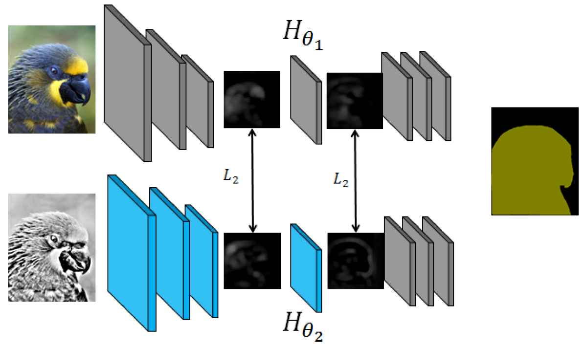
Figure 1: Top: The trained and frozen (gray) network provides ground truth deep representations. Down: The trainable layers (blue) must learn the deep representations.

One application example is environmental monitoring across time [15]: a DCNN is used to segment land categories on aerial images over a period from 1955 to 2015. The 2015 dataset is made of RGB digital images whereas the 1955 data is made of black and white analog images that have been digitized. A network trained on the 2015 data can not generalize on the 1955 one because the images do not have the same color domain nor the same resolution or grain. And even though the surveys cover the same area, the images are not perfectly aligned due to small changes in land use, which prevent the use of 2015 annotations to train a network on the 1955 data. What stays coarsely invariant for one image across surveys is the high-level semantic content.

We emulate equivalent transformations on the PASCAL VOC 12 dataset [5]. Synthetic data is necessary to gather ideal baselines since they require pixel-wise annotated images over several input distribution (Section 3.2). To the best of our knowledge, there is no such dataset publicly available. Experiments show that our transfer method reaches the same performance as standard transfer learning and classic training. Our contribution is twofold: i) we extend the initial work of [1] to semantic segmentation on a wider database, ii) we provide visual insight on the CNN adaptation behavior. The next section describes the state-of-the-art in transfer learning for DCNN. Section 3 and 4 present our method and results.

2 Related work

Domain adaptation through feature transfer is first applied to classification: [7] uses auto-encoders to learn high-level representations of sentiments from various datasets to better classify Amazon reviews. And [1] tackles the challenge of digits classification where some classes are not represented in the training set. Both learn a data transformation that best captures each class’s unique features so that a trained classifier can even process class instances from new domains. This transformation is evaluated with the classification score. One of the best methods relies on unsupervised auto-encoder training that forces the network to capture the relevant features to reconstruct the input.

We draw inspiration from these works and transfer the features maps of a segmentation CNN across data domains. Our work differs from [7, 1] in the target task and the feature learning method. First, contrary to previous classification focus, we test our method on semantic segmentation on the same dataset across time. Also, we tackle a different category of domain adaptation where the output variable is the same but the input pixel distribution varies. Second, we do not follow the previous feature training methods: we use the annotations from one dataset to train a segmentation network, then utilize the features that the network autonomously learned as ground-truth feature representations. For every new segmentation dataset, we force the network to match these representations. This method is semi-supervised since it requires only to match images of the same locations, which can be done during the data collection process using odometry.

Given that [15] did not release their segmentation dataset and [8] only provides odometry datasets, we rely on three synthetic transformations of the PASCAL VOC 12 dataset [5] to test our method. Our transfer learning method reach the same performance as finetuning and standard training.

3 Method

3.1 Training

Let $H_{\theta}$ be a network model with weights $\theta$, $X$ an image and ${\cal F}_{\theta}(X)$ the set a set of feature maps of the network $H_{\theta}$, with ${\cal F}_{\theta}(X)=\left\{F^{l}_{\theta}(X),\;l\in L\right\}$. $H_{\theta_{1}}$ is an instance of $H$ trained with supervision on $D_{1}$. $H_{\theta_{2}}$ is another instance of $H$ first initialized with the weights $\theta_{1}$. $H_{\theta_{2}}$ is then finetuned on image pairs $\left\{(X_{1},X_{2})\subset D_{1}\times D_{2}\right\}$ with the same semantic content but different pixel distributions. The feature maps ${\cal F}_{\theta_{2}}(X_{2})$ must match the corresponding ${\cal F}_{\theta_{1}}(X_{1})$ without ground-truth annotations on $D_{2}$. A loss is computed for each feature map and is back-propagated only in the layers lower than $l$: $\mathcal{L}^{l}(X)=w_{l}\|F^{l}_{\theta_{1}}-F^{l}_{\theta_{2}}\|^{2},w_{l}\in\mathbb{R}$. In our implementation, the feature weights $w_{l}$ are constant over the training. Investigations over dynamic weighting strategies have been left for future work.

3.2 Evaluation

Our transfer method is evaluated with the segmentation performance of the adapted network $H_{\theta_{2}}$ on the new dataset $D_{2}$. We use the standard segmentation evaluataion metrics: the mean accuracy (acc) and the mIOU. We compare against three baselines: baseline $B_{0}$ measures the performance of the first network $H_{\theta_{1}}$ on the new dataset $D_{2}$, i.e. how well $H_{\theta_{1}}$ generalizes to a dataset with the same content but a different pixel distribution. This also gives a quantitative measure of the image transformation between two datasets.In $B_{1}$, we train $H_{\theta_{2}}$ with full supervision on $D_{2}$ using the pixel-wise annotations from $D_{1}$. This ideal setting provides the performance our transfer learning should aim at. The last baseline $B_{2}$ measures the performance of $H_{\theta_{2}}$ when it is initialized with $\theta_{1}$ and then classically fine-tuned on $D_{2}$ with $D_{1}$ annotations. This provides the performance of classic supervised fine-tuning our method should reach while not using explicit annotations.

3.3 Visualization

Besides the proposed domain adaptation techniques described above, this paper also developed a visualization technique inspired from existing approaches used in other contexts. Specifically, we design an optimization to observe the evolution of the representations induced by the feature regression during the domain adaptation. An image $X_{1}\in D_{1}$ is fed to $H_{\theta_{2}}$ to generates a set of features ${\cal F}_{\theta_{2}}(X_{1})$. Starting from white noise, we then generate the image $\hat{X_{1}}$ that minimizes $\sum_{l\in L}\|F^{l}_{\theta_{2}}(X_{1})-F^{l}_{\theta_{2}}(\hat{X_{1}})\|$, i.e. a version of $X_{1}$ as seen by $H_{\theta_{2}}$. Visually, $\hat{X}_{1}$ has the same content as $X_{1}$ with the visual aspect of $D_{2}$.

The optimization is inspired from the feature map inversion method [12] to integrate style transfer into it. In addition, we adapt the style transfer method from [6] [10] to generate image content and style from only one network instead of two. The final optimization is performed as follows: we initialize $\hat{X_{1}}$ with white noise and feed it to $H_{\theta_{2}}$. For each feature map, a content loss and a style loss are computed and backpropagated into the image. $\hat{X_{1}}$ is optimized with Stochastic Gradient Descent (SGD). We use the losses and Gram matrix definitions from [6]. The content loss is a simple $\mathcal{L}_{2}$ loss between feature maps $\mathcal{L}_{content}(l)=\frac{1}{2}\|F^{l}_{\theta_{2}}(X_{1})-F^{l}_{\theta_{2}}(X)\|^{2}$. The style loss is a normalized $\mathcal{L}_{2}$ loss between the Gram matrix of the feature maps. This matrix is computed from a 2D projection of each feature map $F^{l}_{\theta_{2}}$: $\mathcal{L}_{style}(l)\propto\|G(F^{l}_{\theta_{2}}(X_{1}))-G(F^{l}_{\theta_{2}}(X))\|^{2}$.

4 Experiments

4.1 Dataset

We run tests on three synthetic transformations of the augmented version [9] of the PASCAL VOC12 dataset [5] resulting in 10 582 training images and 1449 validation images with 21 semantic classes. The regression is trained on the 10 582 original images of $D_{1}$ and the transformed ones of $D_{2}$. $H_{\theta_{2}}$ is then evaluated on the transformed validation set of $D_{2}$.

Three transformations $T_{1},T_{2},T_{3}$ with increasing perturbations are generated with GIMP resulting in $D^{1}_{2},D^{2}_{2},D^{3}_{2}$ (Figure 2). We use the ’photocopy’ filter $T_{1}$ to emulate a change of color and saturation. This problem arises in long-term environmental monitoring where recent datasets are numerical RGB images and older datasets are collected with the numerization of analogic pictures [15]. We address the issue of image misalignment and noise with the ripple distortion $T_{2}$. This is typical in natural environment monitoring such as in the dataset from [8]. Finally, we mix a change of texture and misalignment with edge noise in the cubism filter $T_{3}$.

Figure 2: Synthetic transformations. Column 0: PASCAL. Left-Right: transformation. Photocopy (Distortion: 32.5%), Ripple (62.6%), Cubism (94.0%)

For each transformation $T_{i}$, the image distortion between $D_{1}$ and $D_{2}^{i}$ is quantized with the normalized performance degradation of the network $H_{\theta_{1}}$ on $D_{2}^{i}$. After training $H_{\theta_{1}}$ on $D_{1}$ with the original DeepLab V3 [2] setup, the accuracy and mIOU reach respectively 79.92% and 69.22%. With $\textrm{acc}(H_{\theta_{1}},D_{2})$ and $\textrm{mIOU}(H_{\theta_{1}},D_{2})$ the performances of $H_{\theta_{1}}$ on $D_{2}$, the image distortion between $D_{1}$ and $D_{2}$ is: $\frac{1}{2}\left(\frac{|79.92-\textrm{acc}(H_{\theta_{1}},D_{2})|}{79.92}+\frac{|69.22-\textrm{mIOU}(H_{\theta_{1}},D_{2})|}{69.22}\right)$.

The dataset distortions (Fig. 2) comfort the visual intuition that the three transformations exhibit an increasing level of complexity that challenges the network trained only on $D_{1}$.

4.2 Experimental Setup

4.2.1 Supervised training of $H_{\theta_{1}}$.

$H$ follows the state-of-the-art VGG-16 architecture [17] from DeepLabV3 [2] for training time considerations. and converges within only 5 hours of training on an NVIDIA 1080Ti. As in [2], we train the network for 20 000 iterations with a batch size of 10, SGD with a momentum of 0.9, a weight decay of 0.5 and the ”poly” learning rate policy initialized at $2.5\times 10^{-4}$ and $power=0.9$.

4.2.2 Feature map training of $H_{\theta_{2}}$.

We run the unsupervised domain adaption training on several sets of ${\cal F}$ to better understand the hierarchical model of network representations.

An intuition gathered from the literature [4, 13, 16] suggests that early layers capture low-level representations such as colors and edges, whereas higher layers embed more complex representations such as object contours and their label. According to this intuition, we could expect that regression of high layers are more relevant than lower ones when the transformation is significant. To test this assumption, we run individual regressions on one feature map and compare the performance of $H_{\theta_{2}}$. We choose the feature map post max-pooling as they show the highest representations shifts in consecutive layers. When we display features of a VGG bloc, the features of successive convolutional layers look highly similar whereas we always observe significant variations after the pooling layers.

We also test the correlations between the network representation levels. We run the regression on all the post-pooling layers simultaneously with two weighting strategies. In the first one, $W_{inc}$, $w_{l}$ increases with the layer level, i.e. we favor the deeper representations. We do the contrary with the second one, $W_{dec}$, and rely more on low-level features. In both cases, we use the following uniform weight distribution $[0.2,0.4,0.6,0.8,0.9]$.

4.3 Experimental Results

Despite training without supervision, our method reaches similar or higher performance than classic supervised fine-tuning (Fig. 3). The feature map chosen for the regression has a high impact on the performance: regression on the higher level maps provides better results (Fig. 4). Figure 5 illustrates how the feature maps of the old network shift toward their initial representations after our finetuning. The image reconstructed from the finetuned feature maps displays the same content as in the old dataset but with the style of the new one (Fig. 6). This observation follows previous findings in neural image style transfer [6]: $\mathcal{L}_{2}$-regression between feature maps does transfer the image content but not the image style.

Quantitative Results

Fig. 3 shows that the regression results on pool5 reach similar performances to classic fine-tuning. The $B_{0}$ line recalls the performance of $H_{\theta_{1}}$ on the transformed dataset $D_{2}$. Our method improves significantly the metrics compared to $B_{0}$ which means that transferring deep representations is indeed a relevant transfer learning method for semantic segmentation. Classic finetuning $B_{2}$ outperforms the training from scratch $B_{1}$ on $D_{2}$: this comforts the results from [11] on the importance of weight initialization and that finetuning is relevant for boosting the performances. Our method always outperforms $B_{2}$’s mIOU and reaches similar mean accuracy. This shows that transfer learning of deep representations can replace classic CNN finetuning without performance degradation.

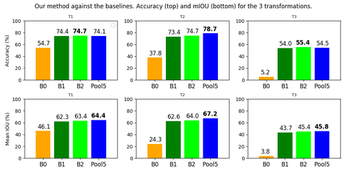
Figure 3: Transfer performance against the baselines.

Fig. 4 summarizes the performances of individual and parallel regressions to better understand the network representation hierarchy. The best performances are reached with the individual regression on the highest post-pooling layer pool5. This suggests that high-level representations are the most relevant to transfer for semantic segmentation. The metrics for each regression vary with the transformation type. The experiments do not allow to draw a general conclusion but we can gather an intuition on which representations are the most relevant to transfer. For the color and saturation transformation $T_{1}$, the transfer of layers up to pool3 improves $B_{0}$ which is not the case for $T_{2}$ and $T_{3}$. One explanation can be that $T_{1}$ conserves the alignment of the image and that color processing is handled in the low-level layers. $T_{2}$ and $T_{3}$ maintain the image color domain but modify the contours of the semantic units either with regular noise as in the ripple transformation or with random one in the cubism effect.

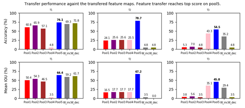
Figure 4: Transfer performance against the transferred features maps. Transferring on pool5 gives the best scores.

Object contours are features usually generated in deeper layers which can explain why the transfer of pool_5 only is relevant for these datasets. These results also suggest that when low-level layers are not relevant to transfer, they can hinder the transfer of the relevant layers. For example, the transfer learning on multiple layers performs worse than the transfer on pool5 only. For $T_{3}$, we observe that a weight distribution that favors high layers performs better than $W_{dec}$ but worse than the transfer of pool5. The overall intuition we can draw consists in relying on high-level feature transfer even though low-level layers can be relevant for color domain perturbations.

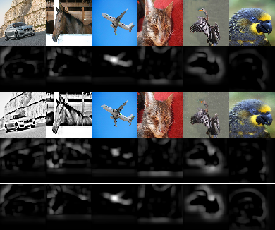
Figure 5: Deep representation evolution. Line 1: original images. Line 2: one feature of the old network $H_{\theta_{1}}$ on the old data $D_{1}$. Line 3: perturbed image from the new data $D_{2}$. Line 4: the same feature of the old network $H_{\theta_{1}}$ on the new data $D_{2}$. Line 5: the same feature of the new network $H_{\theta_{2}}$ on the new data $D_{2}$.

Qualitative Results

Figure 5 illustrates how finetuning shifts the feature maps on the new dataset towards the maps from the old one. The first two lines display the original image and one of their feature maps. The next line displays the perturbed images followed by the same feature map, before and after our finetuning. The new map appears less noisy, especially around the semantic contours of the image. This empirical observation generalises to most of the image feature maps. One possible interpretation is that our adaptation regularises the feature noise introduced by the change in image distribution.

The image reconstructed from the new CNN feature maps displays the visual style of the new dataset (Fig. 6). This interesting observation suggests that the $\mathcal{L}_{2}$ regression of feature maps only transfers image content between CNNS and not the style. The new network is specialised on the new image style. This explanation is coherent with previous image style transfer work [6, 10]: the optimisation run in these work generally have two terms: the first one is a simple $\mathcal{L}_{2}$ between feature maps and is called the ‘content’ loss. The second term, termed the ‘style loss’, is the difference between the gram matrix of the feature maps i.e. the relative relations of the vectors inside one feature maps. Since we only regress the feature maps, it was expected that the new network would embed the style of the new dataset.

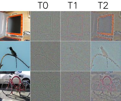
Figure 6: Style reconstruction. The finetuned network is fed with the left-most image. We reconstruct the image as seen by the three finetuned networks (right images). The generated image has the same content and the style on which the network is finetuned.

5 Conclusion

We have introduced a method for unsupervised domain adaptation for semantic segmentation that relies on the transfer of CNN deep representations. It is relevant for applications with redundant semantic content and a drift of the pixel distributions such as autonomous-driving or long-term environment monitoring for which new datasets covering a similar semantic content are acquired over time. This method shows similar performance to classic fine-tuning on three synthetic transformations of the PASCAL VOC dataset that emulates color domain variations, resolution degradation and noise. Quantitative results suggest that high-level representations are the most relevant to transfer even though low-level transfer also reach acceptable performance for color-domain transformations. These observations comfort the recurrent intuitions on the semantics of CNN features.

References

- [1] Bengio, Y. Deep learning of representations for unsupervised and transfer learning. In Proceedings of ICML Workshop on Unsupervised and Transfer Learning (2012).
- [2] Chen, L.-C., Papandreou, G., Kokkinos, I., Murphy, K., and Yuille, A. L. Deeplab: Semantic image segmentation with deep convolutional nets, atrous convolution, and fully connected crfs. IEEE transactions on pattern analysis and machine intelligence 40, 4 (2018), 834–848.
- [3] Cordts, M., Omran, M., Ramos, S., Rehfeld, T., Enzweiler, M., Benenson, R., Franke, U., Roth, S., and Schiele, B. The cityscapes dataset for semantic urban scene understanding. In Computer vision and pattern recognition (2016).
- [4] Dosovitskiy, A., and Brox, T. Inverting visual representations with convolutional networks. In Computer vision and pattern recognition (2016).
- [5] Everingham, M., Eslami, S. A., Van Gool, L., Williams, C. K., Winn, J., and Zisserman, A. The pascal visual object classes challenge: A retrospective. International journal of computer vision 111, 1 (2015), 98–136.
- [6] Gatys, L. A., Ecker, A. S., and Bethge, M. Image style transfer using convolutional neural networks. In Computer Vision and Pattern Recognition (2016).
- [7] Glorot, X., Bordes, A., and Bengio, Y. Domain adaptation for large-scale sentiment classification: A deep learning approach. In Proceedings of the 28th international conference on machine learning (ICML-11) (2011), pp. 513–520.
- [8] Griffith, S., Chahine, G., and Pradalier, C. Symphony lake dataset. The International Journal of Robotics Research 36, 11 (2017), 1151–1158.
- [9] Hariharan, B., Arbeláez, P., Bourdev, L., Maji, S., and Malik, J. Semantic contours from inverse detectors. In Internation Conference on Computer Vision (2011).
- [10] Johnson, J., Alahi, A., and Fei-Fei, L. Perceptual losses for real-time style transfer and super-resolution. In European Conference on Computer Vision (2016).
- [11] Lamblin, P., and Bengio, Y. Important gains from supervised fine-tuning of deep architectures on large labeled sets. In NIPS* 2010 Deep Learning and Unsupervised Feature Learning Workshop (2010), pp. 1–8.
- [12] Mahendran, A., and Vedaldi, A. Understanding deep image representations by inverting them. In Computer vision and pattern recognition (2015).
- [13] Oquab, M., Bottou, L., Laptev, I., and Sivic, J. Learning and transferring mid-level image representations using convolutional neural networks. In Computer Vision and Pattern Recognition (2014).
- [14] Pan, S. J., and Yang, Q. A survey on transfer learning. IEEE Transactions on knowledge and data engineering 22, 10 (2010), 1345–1359.
- [15] Richard, A., Benbihi, A., Pradalier, C., Perez, V., Van Couwenberghe, R., and Durand, P. Automated segmentation and classification of land use from overhead imagery. In 14th International Conference on Precision Agriculture (2018).
- [16] Simonyan, K., Vedaldi, A., and Zisserman, A. Deep inside convolutional networks: Visualising image classification models and saliency maps. arXiv:1312.6034.
- [17] Simonyan, K., and Zisserman, A. Very deep convolutional networks for large-scale image recognition. arXiv:1409.1556.