Late Bloomer Galaxies: Growing Up in Cosmic Autumn

Abstract

Late bloomers are massive ($M_{\ast}>10^{10}\,\rm{\hbox{$\,$M${}_{\odot}$}}$) galaxies at $z<1$ that formed the majority of their stars within $\sim$2 Gyr of the epoch of observation. Our improved methodology for deriving star formation histories (SFHs) of galaxies at redshifts $0.45<z<0.75$ from the Carnegie-Spitzer-IMACS Survey includes confidence intervals that robustly distinguish late bloomers from “old” galaxies. We use simulated SFHs to test for “false positives” and contamination from old galaxies to demonstrate that the late bloomer population is not an artifact of our template modeling technique. We show that late bloomers account for $\sim$20% of $z\sim 0.6$ galaxies with masses of the modern Milky Way, with a moderate dependence on mass. We take advantage of a 1% overlap of our sample with HST (CANDELS) imaging to construct a “gold standard” catalog of 74 galaxies with high-confidence SFHs, SEDs, basic data, and HST images to facilitate comparison with future studies by others. This small subset suggests that galaxies with both old and young SFHs cover the full range of morphology and environment (excluding rich groups or clusters), albeit with a mild but suggestive correlation with local environment. We begin the investigation of whether late bloomers of sufficient mass and frequency are produced in current-generation $\Lambda$CDM-based semi-analytic models of galaxy formation. In terms of halo growth, we find a late-assembling halo fraction within a factor-of-two of our late bloomer fraction. However, sufficiently delaying star formation in such halos may be a challenge for the baryon component of such models.

1. Introduction: Star Formation Histories, Individual and Collective

The global history of star formation is constructed by measuring the star formation rate (SFR) of galaxies over cosmic time in a sufficiently large volume to contain a representative sample of starforming galaxies. The evolution of this quantity, the star formation rate density, (SFRD; Lanzetta, Wolfe, & Turnshek 1995, Lilly et al. 1996, Pei & Fall 1995, Madau & Dickinson 2014, hereinafter MD14), is well defined over most of cosmic history, $0<z<10$ (Oesch et al. 2014). Modulo corrections for starlight absorbed by dust grains and potential incompleteness from galaxies fainter than—and SFRs less than—the observation limit, the SFRD is an accurate description of the efficiency with which galaxies have grown since a time when their stellar masses were $\sim$1% of what they are today. The cumulative buildup of stellar mass, recovered from the mass function of galaxies over the same range of epochs, is in good agreement with the integral of the SFRD (Dickinson et al. 2003; MD14). It could be argued, then, that the story of global stellar mass production is now reasonably well understood, or at least well-characterized.

“Cosmic noon” is a good name for when the luminosity of the universe peaked (as is “cosmic dawn”—first light). However—as suggested by the title of this paper—the growth of galaxies relates better to cosmic seasons rather than hours of the day; i.e., a cosmic spring ($3<z<6$), summer ($1<z<3$), and autumn ($z<1$). with cosmic winter yet to come.

In their comprehensive review of the history of cosmic star formation, MD14 parameterized the rise and fall of the SFRD as a polynomial (see MD14 Figure 9, Equation 15), a form that provides a good fit to the data but offers no insight into the physical processes that control the evolution of the global SFR, let alone the SFR histories of the individual galaxies from which it is composed. Taking this latter step requires a further constraint on the behavior of SFRs with epoch. The star formation main sequence (SFMS; e.g., Noeske et al. 2007; Whitaker et al. 2012)—a now thoroughly studied correlation between stellar mass and SFR at $z\lesssim 6$—has been the favored method for constructing SFHs that, in aggregate, reproduces the SFRD (e.g., Peng et al. 2010, Speagle et al. 2014, or Tomczak et al. 2016). From the near-unity slope of the SFMS the implication has been drawn that galaxies grow in direct proportion to their mass, modulo the rising zero point of the SFMS before $z\sim 2$—faster growth—and a rapid decline after. If the considerable scatter of the SFMS can be taken as a series of random perturbations on otherwise smooth growth, each galaxy can be fit by a set of conformal growth curves, identical up to a mass scaling (e.g., Peng et al. 2010, Leitner et al. 2012; Behroozi et al. 2013). However, since the SFMS bends from this unity slope at its high mass end—in effect, a general slowing of the stellar mass growth after the peak in the SFRD—some sort of “quenching” mechanism is required to explain the declining SFRs of evolved, massive galaxies, and its collective manifestation in the decline of the SFRD after $z\sim 1.5$.

In a previous series of papers, Oemler et al. (2013, O13), Gladders et al. (2013, G13) Abramson et al. (2015), Abramson et al. 2016, A16), and Dressler et al. 2016, D16), we have described a different approach that evolved from O13’s identification of a fraction of massive galaxies, $\log M_{\ast}\gtrsim 10.6$, increasing in redshift up to $z\sim$1, that require rising SFRs around the epoch of observation (T_obs). This is a notable departure from what had long been inferred from studies of low-redshift galaxies: almost every present-day galaxy can be fit by a “tau-model” of exponential decline (Tinsely 1972). O13 found a fraction of these so-called “young” galaxies of $\sim$20% by $z\sim 0.8$. Such galaxies had been found in previous studies (e.g., Cowie 1996, Noeske et al. 2007), however, the larger sample of O13 showed that their prior characterization as starbursts was not tenable (see Figure 4 of O13). Although late-rising SFHs are observed for many present-epoch dwarf galaxies (e.g., Gallagher et al. 1984), the identification of rising SFRs for a substantial fraction of massive galaxies ($M_{\ast}>10^{10}$ M_⊙) at redshifts $z>0.3$ was new information for understanding the evolution of common galaxies (see, for example, Kelson 2014).

Responding to the inadequacy of tau-model SFHs for this population, Gladders et al. (2013; G13) explored the idea that individual SFHs might be better parameterized by a two-timescale lognormal form. This idea that came from realizing that the SFRD itself is well described as a single lognormal, with timescales of $T_{0}\approx 5.2$ Gyr (associated with the midpoint of mass buildup), and a characteristic duration of 5.7 Gyr.

Abramson et al. (2015) and A16 explored the implications of this parametric SFH model in terms of the galaxy stellar mass function. These studies found a very good match even up to $z\sim 8$, remarkable because the parameters of the G13 model relied only on data from galaxies at redshifts $z<1$. A16 expanded this to include the slope, evolution, and scatter of the SFMS and other aspects of the SFMS “grow and quench” picture, finding again that the G13 lognormal SFHs model accounted equally well for observations of principal ensemble behaviors. The paper concluded that identifying a uniquely “good” description of galaxy evolution required new observational constraints.

Towards this end, D16 investigated individual galaxy spectral energy distributions—SEDs—and their implied SFHs in order to test the efficacy of the two approaches, which to that point were evaluated mostly in terms of distribution functions and scatter-plots/scaling-laws. D16 used spectrophotometric data from the Carnegie-Spitzer-IMACS study (CSI, Kelson et al. 2014, K14) that combined broad-band photometry and IMACS (Dressler et al. 2011) prism observations for $\sim$20,000 galaxies in the XMM field of the Spitzer SWIRE survey (Lonsdale et al. 2003). These data were used to construct SEDs analyzed in terms of SFHs. The innovative methodology of K14 was to model the SED as the sum of 6 epochs of (constant level) star formation, the first from redshift $z=5$ to 1 Gyr before the epoch of observation, T_obs, followed by five 200 Myr periods over that final Gyr. D16 defined a quantity z5fract as the fraction of the total stellar mass generated before the final Gyr of the observed galaxy. Using z5fract as a proxy for the galaxy’s mean age brought attention to a population of late-growing galaxies with a fraction of old stellar mass—i.e., that formed in the first SFH bin—below 50%. This population amounted to about 20% of the sample, reminiscent of the fraction of young galaxies found in studies cited above and the G13 model analysis. D16 was a step beyond the earlier work, though, because the identification of individual SFHs, while crude, offered for the first time the possibility of discriminating between the “grow and quench” and “a diversity of lognormals” pictures.

In this paper, we improve and refine the SFH analysis of D16, focusing on the reality of what we called “late-bloomers,” galaxies at $z\sim 0.6$ where the majority of its stellar mass appears to have formed later than $z\sim 1$. (See Chauke et al. 2018 for a recent complementary study at $z=0.6$–1.) This includes a critical look at the possibility that our earlier analysis simply failed to detect large populations of old stars because of insufficient sensitivity or the hiding of these stars by dust. By exploiting the highest signal-to-noise ($S/N$) data of the CSI XMM field and making full use of the thousands of duplicate measurements collected in the survey, we arrive at a improved SFH analysis, particularly with respect to the amount of old stellar mass in what appear to be genuinely young galaxies. Further, we add confidence intervals to the SFHs to accurately characterize their uncertainties, and perform a rigorous analysis of simulated SEDs to assess the impact of $S/N$ on SFH derivations and to determine the level at which late bloomers might be contaminated by misidentified older objects.

With measures of confidence in our SFH fits of CSI data, we catalog a “gold sample” of 74 galaxies with high confidence SFHs and HST (CANDELS) imaging. We provide coordinates and other basic data, including RGB images, SEDs, and derived SFHs to enable other researchers to observe and analyze these galaxies and compare their results with ours.

Indeed, new datasets and methods now make this kind of analysis not only possible, but robust (see, e.g., Pacifici et al. 2012, 2016; Iyer & Gawiser 2017; Chauke et al. 2018). Extant and future facilities can support inferences regarding the full diversity and character of individual galaxy growth and so directly confront theoretical evolutionary models in their native domain. This work joins the above cohort of complementary studies in establishing the first more-than-tentative footholds in this new regime.

The paper is organized as follows: Section 2 reviews the methodology of D16 in the context of the fidelity of the SEDs. There, we define “late bloomer” (Section 2.2), and describe improvements to the analysis made through a purposeful attempt to falsify our claim that such galaxies are common and span a wide range in stellar mass. Such careful scrutiny and skepticism are justified by the challenge late bloomers may present to conventional wisdom about the growth of stellar mass. Section 3 presents our best assessment of the global late bloomer fraction at $z\sim 0.65$. Section 4 presents the catalog of 74 galaxies with HST imaging, secure SEDs, and high-confidence SFHs, intended to encourage tests of our results with other techniques and analyses. Section 5.1 describes basic properties of late bloomers using larger sample of $\sim$7600 galaxies of $M_{\ast}>10^{10}$  M_⊙ with high-quality SEDs and well-constrained SFHs to explore the late bloomer fraction trends with stellar mass, redshift, and environment. The discussion in Section 5.2 focuses on the compatibility of late bloomers with a $\Lambda$CDM semi-analytic model of stellar mass growth, including the implications of this work for abundance matching and scaling laws as tools in studying galaxy evolution. Section 6 distills the major conclusions of the paper and describes possible next-steps—including ongoing efforts to obtain higher resolution IMACS spectra—to significantly improve SFH constraints and better distinguish late bloomers from truly old galaxies.

2. Improvements in Deriving SFHs from CSI Spectrophotometric Data

The results of D16 on SFH diversity were not anticipated in designing the CSI program. Its primary goal was to improve on previous measurements of the fraction of passive galaxies as a function of redshift and stellar mass, in connection with the question of which processes might lead star forming galaxies to a temporary or permanent cessation of star formation. Because passive populations are most luminous in the near-IR, the choice of a sample from the SWIRE project, magnitude-limited by Spitzer 3.6 $\micron$ imaging, yielded improved sensitivity to passive populations at redshifts up to $z\sim 1.5$ and thus a better measure of the evolution of their fraction of the total galaxy population.

The goal in CSI of measuring redshifts to 2% or better—important both for SED analysis and for distinguishing galaxy clustering—led to a better method of extracting SFHs from the combination of IMACS prism spectra and broad-band photometry. This necessarily included an accurate assessment of star formation in the final Gyr before the epoch of observation (T_obs), as distinct from earlier star formation. This in turn lead to the parameterization of the SFH as a single early epoch of star formation beginning at $z=5$ followed by 5 epochs of 200 Myr duration in the final Gyr. Slicing cosmic history in this way well addressed the question of whether galaxies were passive or active and provided, for passive galaxies, potential evidence of relatively recent star formation. Such information that might inform the mechanism of what is commonly called “quenching” of star formation.

The fraction of stellar mass a galaxy produced in the Gyr before T_obs was a matter of special interest because of O13’s study of field galaxies (in the IMACS Cluster Building Survey) that inferred rising SFHs for a growing fraction of galaxies at redshifts $0.2<z<0.8$. Rising SFHs were implied by specific star formation rates (sSFRs) that exceeded what is allowed for constant star formation systems—the limiting case for exponentially declining “tau-model” (Tinsley 1972). The CSI data moved this work beyond a comparison of sSFR distributions at different epochs to the actual identification of galaxies with rising SFHs after $z\approx 1$.

In fact, such rising SFHs are implied by characteristic SFRs that are twice the lifetime average of galaxies (e.g., Kelson 2014, see also G13). The importance of such results is easy missed. Even modest fractions of galaxies with late-rising SFHs imply a break in mass rank ordering, making traditional techniques of abundance matching an exercise that is dubious, at best. The implication that the relative positions of galaxies within scaling relations like the SFMS do not stay fixed vitiates any ability to connect progenitors and descendants over cosmic time using scaling relation data and stellar masses alone.

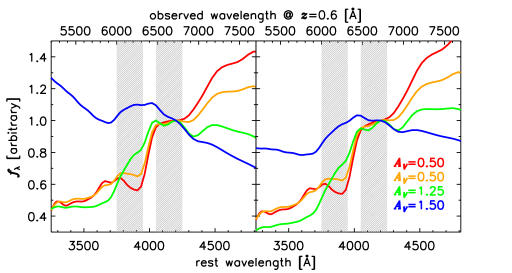
Figure 1.— Four template SEDs for solar metallicity stellar populations with a range of ages. (left) SEDs of population unattenuated by any dust; (right) the same SEDs but attenuated by levels of dust given in the figure. The blue line is a young population, constant SFR from 200 Myr prior to T_obs; green line, from 1 Gyr to 200 Myr; orange line, from 2 to 1 Gyr; red line, from $z=5$ to 2 Gyr before T_obs. Populations 1 Gyr or younger are easily distinguished from older populations, while 1–2 Gyr, though less distinct, has a significantly different SED than that of constant star formation from $z=5$ to $z=1$ (or star formation that ended earlier). Adding a 1–2 Gyr epoch of star formation into the CSI SFH modeling enables the recovery of a longer timescale of late star formation, as is expected given our knowledge of the SFHs of the Milky Way and its neighbors inferred directly through color-magnitude diagrams. Each template is normalized at rest-frame 4200 Å; vertical dashed lines show bandpasses measuring the D4000 break at $z=0.6$. Even when the young populations are highly reddened, SEDs have structure, around the Balmer and 4000Å breaks for example, that provide strong leverage on the relative fractions of old, intermediate, and young stellar mass.

After D16, we recognized the advantage of pushing further back in time—from 1 Gyr before T_obs to 2 Gyr—effectively separating the old from young stellar populations at $z\approx 1$ (given the sample $\langle z\rangle\sim 0.6$). Figure 1 shows that the stellar template of a 1–2 Gyr old population, essentially F stars, can be distinguished from the template of the $\sim$5 Gyr of old stars that preceded it. By adding this epoch of intermediate-age star formation, our analysis has purchase on star formation after $z\approx 1$ that occurred prior to the easily recognizable 0–1 Gyr population. Furthermore, our new model SFHs are less likely to incorrectly ascribe star formation that is relatively recent to the oldest stellar population. We discuss the 1–2 Gyr population further in Section 2.1.

Figure 2 (top) shows our new scheme for parsing SFHs into five age intervals: (1) constant SFR from 200 Myr prior to T_obs; (2) 500 to 200 Myr; (3) 1 Gyr to 500 Myr; (4) 2 to 1 Gyr; (4) from $z=5$ to 2 Gyr before T_obs. In addition to better time resolution of SFHs back to $z\approx 1$, these choices represent an improvement over the four equal-length time bins because they are attentive to the natural timescales of stellar populations as expressed in stellar spectra.

Figure 2 also explains how the SEDs are presented in Section 4. The constraining data are photometry in 8 broad bands (ugrizJK_s—the red boxes) and an IMACS prism spectrum covering (rest-frame) 3000–4500 Å (the blue trace). The solid black line shows the best fit to the photometry and spectrum produced through the modeling. The five components to the model SED are shown as template spectra at the derived flux level for each age bin where star formation has been detected. The templates are color-coded to match the SFRs and integrated stellar mass, as shown in the enlarged left and center boxes above the upper SED. The modeling also solves for $A_{V}$ extinction (right-center box, following Calzetti et al. 2000) and metal abundance (not shown) for each of the stellar populations.

The two example CSI SEDs shown in Figure 2 from the statistical sample (see Sec 3) span the wide diversity of SFHs found by D16. The upper example is a $z=0.62$ galaxy dominated by an old stellar population, the kind of galaxy that has long been recognized in this subject. It is noteworthy, however, that this very massive galaxy is not “quenched,” but shows a continuing history of star formation that, in the best fitting model, adds $\sim$25% in stellar mass since $z\approx 1$. The lower example is a $z=0.586$ galaxy dominated by star formation after $z\approx 1$. Active star formation is well detected in both galaxies, beginning 500 Myr before T_obs, and accompanied by 1.3–1.5 magnitudes of extinction.

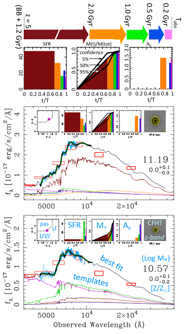
Figure 2.— Two example SEDs from CSI. At the top of the figure are the 5 “age bins” (in order of decreasing age, the brown, orange, green, blue, and magenta arrows) used to parameterize the SFH. Each SED includes: (1) the data—broad band photometry (8 red boxes; Spitzer 3.6 $\mu$m fluxes were used for selection only, not in SED fitting) and the IMACS prism spectrum (blue trace); (2) the most-likely SED fit (black line); (3) stellar templates for constant star formation in the five color-coded age intervals; (4) $\log M_{\ast}$; (5) the metal abundance of the fit model. The thin black line is the maximum likelihood fit—the sum of the templates, but at the lower spectral resolution of the prism data. The width of the heavier line through the prism data covers the 5%–95% uncertainty of the fit model. The five boxes above the SED show: (1) UVJ diagram (passive vs active SF); (2) the mean SFR over each age interval (SFH); (3) fractional stellar mass growth; (4) extinction ($A_{V}$ mag) for each age interval; (5) isophotal $z$-band image from CFHT Legacy Survey. The three black lines in the center box show the confidence interval derived for stellar mass growth—5%, maximum likelihood, 95%. The top SED shows a well-constrained SFH; nevertheless, the range of 60%–95% contribution from the old population (born 2 Gyr or more before T_obs) covers both a dominant old galaxy and one that has formed stars more-or-less constantly up to T_obs. The bottom SED has a confidence interval that appears wider, but an old contribution of less than 50% (built up in $\sim$5 Gyr compared to 2 Gyr) identifies this galaxy—with high confidence—as a late bloomer.

However, the “best fit” model of the SED is not the whole story. The most important modification of our approach since D16 is the extraction of confidence intervals for the SFHs, which previously had been recorded only as the fit of maximum-likelihood (ML). Adding the bounding values that specify the 5% and 95% confidence fits provides an essential metric of SFH reliability. Focusing on the center box (the stellar mass growth), we see that the SFH of the top SED constrains the population of stars older than T_obs– 2 Gyr to between 60% to 95% of the stellar mass. In other words, our confidence interval runs from a galaxy that is almost completely old to one that has essentially “constant star formation” from $z=5$ to T_obs. The 5%–95% confidence interval for the bottom example runs from a galaxy with zero old stellar population to one with as much as $\sim$35%. Either way, this galaxy is found to be very young, despite its Milky Way (MW)-like mass (i.e., $\log M_{\ast}\in[10.5,10.8]$).

We use these SFH confidence intervals in the following discussion to define a class of massive galaxies that has not been recognized: massive $z\sim 0.6$ galaxies whose stars formed mainly within 2 Gyr following $z\sim 1$, instead of the preceding $\sim$5 Gyr. We call these “late bloomer” galaxies.

2.1. Why Add a 1–2 Gyr Stellar Template?

Figure 1 shows that stellar populations of age $\mathrel{\raise 1.50696pt\hbox{$\scriptstyle<$}\kern-6.00006pt\lower 1.72218pt\hbox{{$\scriptstyle\sim$}}}$1 Gyr can be unambiguously separated from the light of much older stars. D16 used this as a conservative, reliable way to distinguish young from old populations. However, from the vantage point of galaxies observed $\sim$5 Gyr earlier than today, with their lower fraction of very old stars—all less than 7 Gyr old—a 2 Gyr separation of old and young populations is feasible given sufficient $S/N$, as Figure 1 also shows.

There are good reasons for adding 1–2 Gyr-old stars to the “young” category. First, separating “young” from “old” populations at 1 Gyr made it likely that a significant fraction of recent star formation, 1–2 Gyr before T_obs, was erroneously credited to a population that was, on average, much older. This is mitigated by defining old as “stars forming earlier than 2 Gyr before T_obs.” Second, the identification of late bloomers based on populations less than 1 Gyr from T_obs implied an almost bursty history, while it is more sensible to expect this late epoch of star formation to have lasted several Gyr (e.g., Chauke et al. 2018). Even if the timescale for mass growth is as short as $\sim$1 Gyr, this is far from the conventional situation of incremental mass growth in a burst, since the mass growth has been sufficient to surpass the mass of old stars, those born prior to 1 Gyr, or now, 2 Gyr. In the appendix we show, through the analysis of simulated SFHs, that detections of 1–2 Gyr-old populations are generally reliable, and thus an improvement in identifying late bloomers.

2.2. The Re-Definition of a “Late Bloomer”

Based on the addition of the 1–2 Gyr star formation template, we thus revise the definition of a late bloomer used in D16 based on z5fract—the fraction of mass formed earlier than 1 Gyr before T_obs—to one based on z5fract2, the fraction of mass formed 2 Gyr or more prior. Table 1 (see Section 4) includes z5fract2 and recalculated z5fract values based on our new SFHs, with the modifications described above.

Formally, we define a late bloomer as a galaxy in which $\leq$50% of the stellar mass formed in the epoch $z=5$ to 2 Gyr before T_obs at the 95% confidence level; i.e.,

$${\it z5fract2}_{95\%}<0.5$$ (1)

Through this definition—which our simulations show leads to the best compromise between sample purity and completeness (see the appendix)—mass growth in the final 2 Gyr for late bloomers exceeds that of the previous 5 Gyr. Obviously, this implies rising SFRs (i.e., accelerating mass growth). Moreover, though, it implies SFRs are rising faster than linearly at these epochs: if ${\rm SFR}\propto t$, $M_{\ast}(t)\propto t^{2}$, for which it so happens that z5fract2 $\simeq\,0.5$ at $z=0.65$. This means that our late bloomer definition is conservative—it excludes galaxies that have substantial (though not super-linear) increases in SFR over the final 2 Gyr. As such, our abundance estimates for late bloomer-like systems should be higher than what we quote in Section 3.

Although the galaxies on the other side of this divide are dominated by star formation before $z\sim 1$, our data strongly suggest that not all of these followed similar SFHs that were at some point quenched on a $\mathrel{\raise 1.50696pt\hbox{$\scriptstyle<$}\kern-6.00006pt\lower 1.72218pt\hbox{{$\scriptstyle\sim$}}}$1 Gyr timescale. Rather, we see these older galaxies as including those whose star formation rose and and fell rapidly in the first few Gyr of cosmic history, and those that rose slowly with more-or-less continuous star formation until $z\sim 0.6$—if not all the way to the present epoch. For the purposes of the following discussion, we define old galaxies as those with ${\it z5fract2}\ \geq 0.85$, and constant-star-formation galaxies as forming 50%–85% of their mass before $\hbox{\emph{T${}_{\rm obs}$}}-2$ Gyr ($0.5<{\it z5fract2}<0.85$). The latter interval begins with SFRs that are rising in the final 2 Gyr (not super-linearly) and ends with SFRs that peaked before $z\approx 1$ and are slowly declining by $z\sim 0.6$.

2.3. Spectral Characterization of Late Bloomers

Outfitted with an improved toolkit for turning SEDs into SFHs, we focused on the major issue of the relative proportion of young to old stellar populations in our sample galaxies.

Much of the leverage for deriving a SFH from a SED rests in the low-spectral-resolution ($R\sim 30$) prism spectrum, which is particularly sensitive to young and intermediate-age populations, and the 4 broad-band photometric indices i, z, J, K that measure the contribution from the red-giant-branch stars of old stellar populations. (The Spitzer 3.6 µm detection band is omitted in the SED fitting to avoid selection bias.) Galaxies with star formation during the 2 Gyr before T_obs (since $z\approx 1$, for our sample) show unambiguous evidence through the Balmer break, primarily from A stars, but also from F stars. This signature is readily distinguishable from the contribution from older stars to this spectral region, which exhibits a strong D4000 break and other prominent features—the G-band, Ca H&K lines and CH complexes. (This spectral region is called the “break region” in the discussion to follow.) Massive galaxies can have substantial contributions from both old and young stars, so the spectral resolution $R\sim 30$ of the prism observations is an important advantage over broad-band photometry SEDs in distinguishing the contributions of both young and old populations.

The old stellar population (i.e., older than 2 Gyr at T_obs) dominates the flux further into the red and infrared, so good broad-band photometry beyond 6000 Å is generally sufficient for assessing their contribution. However, the added constraint of the break region may be essential if the older population is viewed through a dusty disk, which can further diminish or eliminate its signature at rest-frame $\lambda\sim 4000$ Å. Since testing the reality of late bloomers depends critically on whether or not an old stellar population can be detected, we tested the dust attenuation issue through simulations of mock spectra that included substantial “hidden” old stellar mass. These tests are summarized in the appendix and included in our full sample result uncertainties (Section 3). The upshot is that the impact of such hidden mass is unlikely to be dramatic, such that the observed late bloomer abundance is accurate to roughly $\pm 0.05$ in absolute terms over a wide range of $S/N$, $A_{V}$, and ${\rm SFR}(\hbox{\emph{T${}_{\rm obs}$}})$ mixes.

2.4. Role of Duplicate Observations

CSI has a $\sim$20% repeat observation fraction to facilitate empirical estimates of measurement errors, which can be nonlinear functions of the observations. In general, these duplicates can unfortunately not be used to test the repeatability of binary classifications such as being a late bloomer. Such groupings are like a biased coin toss, with the bias set by the selection method’s purity. In our case, simulations suggest (and the assessments below reveal) a $P\simeq 70\%$ purity, which is not close enough to unity to guarantee repeat classifications ($\propto P^{n_{\rm obs}}$) agree. Indeed, at $P=0.7$, we expect to repeat-confirm only 58% of the initial late bloomer candidates.

The proper use of repeat observations at moderate purity is instead to characterize formal measurement errors in a continuous—not binary—property. This is analogous to repeated flux measurements in noisy images: the scatter between them reflects the true underlying noise level. In the context of late bloomers, the analogy is repeated assessments of the amount of old stellar mass in a galaxy. The scatter between estimates reflects the noise floor on this estimate. Our classifications should be reliable if this floor is $\lesssim$50%. Fortunately, this is the case.

Averaged over total stellar masses $10\leq\log M_{\ast}^{\rm tot}\leq 11$, the RMS scatter in the differences of maximum likelihood old stellar mass fractions across duplicates is $74\%\pm 2\%$. Assuming Gaussianity, this is $\sqrt{2}\times$ the formal error on a single measurement, implying an acceptable $52\%\pm 1\%$ 1 $\sigma$ noise floor on z5fract2. If these estimates are restricted to galaxies whose first observation implied identically zero old mass, the noise floor—closer to a real upper limit on z5fract2 in these cases—drops to $46\%\pm 2\%$.

As discussed above and in the appendix, however, we do not select late bloomers using the maximum likelihood old mass fractions, but their estimated 95% upper limits. For galaxies with zero maximum likelihood old mass, we find the mean of these limits in the second observation to be $75\%\pm 3\%$ ($10\leq\log M_{\ast}^{\rm tot}\leq 11$). For Gaussian noise, this is $1.960\times$ the standard deviation, implying just a $38\%\pm 1\%$ z5fract2 1 $\sigma$ noise floor. Including all galaxies raises this to $48\%\pm 1\%$.

In sum, both duplicate-based approaches support the conclusion that our LB selection method is accurate at the 1 $\sigma$/68% level. Reassuringly, this is fully consistent with the $\sim$70% purity we infer from simulations (see the appendix).

Comparing duplicate observations and SFHs also helped us optimize our SED fitting, modifying the procedure described in K14 by narrowing dust and metallicity constraints for the oldest population. This allowed finer parameter grids, which improved redshift estimation accuracy. Because of the similarity in shape and location of the Balmer break in young populations and the 4000 Å break in old populations, better redshifts led to higher fidelity SED-derived SFHs.

3. The Late Bloomer Fraction of CSI Galaxies at z $=0.6$

In this section we quantify the fraction of CSI galaxies that were late bloomers $\sim$6 Gyr ago. This measurement simply entails summing the weights of the relevant galaxies, described in K14. Every galaxy’s weight is the inverse of the completeness estimated for its magnitude, color, and local source density, divided by the number of times a galaxy was observed. The CSI late bloomer fraction (LBF) is therefore the sum of the weights for galaxies with ${\it z5fract2}_{95\%}<0.5$ over the sum of the weights of the galaxies in the full catalog. In order to ensure fidelity in late bloomer fraction estimates, we reduced the size of the full XMM-SWIRE CSI catalog of 50,000 high quality redshift measurements to approximately 22,000 systems with high-quality observations and stellar masses above $10^{10}\,\rm{\hbox{$\,$M${}_{\odot}$}}$.

To assess the LBF’s sensitivity to sample depth, $S/N$, redshift uncertainty, and spectrophotometric quality variations, we used seven different versions of the CSI dataset based on different cuts in these dimensions. We fold the RMS scatter (a few percent) between LBFs from these different selections into the error bars in our plots. These different versions of the catalogs are valid statistical samples with their own completeness estimates as functions of magnitude, color, and source density, with sizes ranging from 8,000 to 12,000 galaxies with $M_{\ast}>10^{10}\,\rm{\hbox{$\,$M${}_{\odot}$}}$ at $0.45<z<0.75$. For the measurements of LBF evolution (Section 5.1.2), this sample is extended over $0.25<z<0.75$ and is 25%–30% larger, depending on the selection cuts.

Figure 3.— Late bloomer fractions at $0.45<z<0.75$ in three different stellar mass bins. A substantial fraction of galaxies at these epochs had recently experienced runaway growth. Open circles: Raw CSI measurements; Filled circles: Reasonable lower bounds on true LBFs based on simulations in the appendix; Open squares: Pessimistic lower bounds assuming the raw measurement at $\log M_{\ast}\sim 11$ represents only false positives. The upper dashed line trace 1-$\sigma$ upper bounds on the observed LBFs. The upper solid line includes an additional $\pm 0.05$ uncertainty in those upper bounds due to potential uncertainties in the correction factors to LBFs, as derived from scatter between different simulations of CSI data. While the filled circles trace reasonable lower bounds on the LBFs, using plausible corrections to the measurements, the lower dashed line is the 1-$\sigma$ lower bound on these corrected LBFs from the formal errors alone. The lower solid line includes an additional uncertainty of $\pm 0.05$, derived from scatter between different simulations of CSI data.

Figure 3 shows the measured LBFs as functions of stellar mass at $\langle z\rangle=0.6$ (open circles). Simulations of CSI data described in the appendix allow us to quantify the systematic bias in these measurements due to contamination by false positives (galaxies that grew less than half their mass in the last 2 Gyr). According to these simulations, this bias is approximately zero if late bloomers are selected using the 95% upper limits on z5fract2—the definition we adopt (Equation 1)—with an additional uncertainty of $\pm 0.05$ due to model-to-model variations, uncertainties in the mix of quiescent and star-forming galaxies, and uncertainties in the underlying mix of SFRs at T_obs.

The simulations also let us construct plausible lower limits to the LBFs, with systematic contamination at levels of $+0.05$ for quiescent galaxies and $+0.10$ for star forming galaxies. These plausible lower bounds are shown in Figure 3 using the filled circles.

A third, empirical, and more pessimistic approach is to assume that all late bloomers in the stellar mass bin $\log M>10.8$ are false positives, such that the LBF in that mass bin is identical to the contamination rate (at least for populations with the same mix of quiescent and star forming galaxies). By scaling the high mass LBF by the ratio of the quiescent fraction in each bin to that at high mass, we can empirically correct each bin for the potential contamination by false positives. These results are shown by the open squares.

Formal uncertainties in the raw measurements are estimated through bootstrapping. Systematic uncertainties in those measurements are estimated using the RMS variation in LBF derived from multiple variations of the CSI catalog tailored in different ways, such as varying $S/N$ restrictions, prism spectral quality, how well the spectra have colors that match the photometry, etc. The dashed lines show their quadrature sum above and below the raw measurements and plausible lower bounds. The additional uncertainty of $\pm 0.05$ due to model-to-model variations, uncertainties in the true mix of quiescent and star-forming, and uncertainties in the underlying mix of ongoing star formation rates, added in quadrature, is thus shown by the solid lines.

Taking these measurements at face value, several striking conclusions are readily apparent:

• Many galaxies at least doubled their stellar mass between $z=1$ and $z=0.6$.

• About $20\%$ of MW-mass galaxies did this, and $\sim$30% of galaxies at half the MW’s mass.

• More massive galaxies do this less, but, even at $M_{\ast}>M^{*}$, the LBF remains $\sim$5%–10%.

These relatively simple observations strongly confront the basic picture, commonly held, that most galaxies in this mass range generally grew early, with much slower rates of growth after cosmic summer. They strongly contradict paradigms in which galaxies are thought to simply grow along the SFMS and quench en masse: Even modest numbers of galaxies—to say nothing of 20%—with sustained, rapid, late growth, as shown above, have strong consequences for analyses of galaxy evolution that rely on the preservation of mass (and so abundance) rank ordering.

Given the strong implications for these measurements, we devoted great effort to simulating CSI data with the aim of understanding how to make late bloomers “go away.” That is, we tried to identify what fraction of CSI late bloomer identifications could be due to noise and, for example, dust effects, which could systematically hide old stellar mass and artificially make intrinsically non-late bloomers appear as late bloomers. The simulations allowed us to derive plausible corrections to the CSI measurements, but did not in any way indicate that these were substantially biased by errors in the SED-inferred SFHs.

The upshot of this exercise is that the $z\sim 0.6$ LBF is highly unlikely to be zero for galaxies with stellar masses at least up to $\log M_{\ast}\sim 10.8$. Our most conservative assessment is that the LBFs of galaxies with half-to-all the MW’s mass is at least 10%–20%. Stated most plainly, roughly one-in-five of today’s MW-mass galaxies went through an extreme growth spurt between $z=1$ and $z=0.6$, having evolved only lackadaisically before then, and perhaps since. This is an odd conclusion from the standpoint of SFMS-integration or abundance matching, but, try as we may, we cannot avoid it.

The simulations only provided one scenario to make our LBFs a complete procedural artifact: forcing half the stars to have been formed in the first 1–2 Gyr, to be hidden or partially obscured underneath the stars that formed subsequently. But even even in these cases, the inferred SFHs from the SED fitting represent the formation histories of the final $\sim$5 Gyr. The implication is that such galaxies would have had lacunal histories: initial early “bursts,” rising again only much later to rapidly grow the final quarter of their stellar mass in the 2 Gyr prior to $z\sim 0.6$. To contrive that all late bloomers—again, 20% of MW-mass systems—grew that way seems at least as challenging as accepting them as real late bloomers in the sense of Gladders et al. (2013), Kelson (2014), or Kelson, Benson, & Abramson (2016; hereafter KBA16).

4. A Catalog of Galaxies with HST Imaging and Secure SFHs

This section provides a catalog of galaxies with high-confidence SFHs to serve as a reference sample for comparison with and by other studies. The 5 square degrees of the XMM-SWIRE field containing the sample in this paper overlaps by $\sim$1% with CANDELS HST imaging (Koekemoer et al. 2011). We chose to focus on this area for our catalog since high-resolution images of the calibrator galaxies should be indispensable in evaluating SFHs in terms of galaxy structure and morphology, the presence of near neighbors, distribution of star formation, and notable features (for example, tidal tails) that could be identified. Images also set the stage for later observations and studies motivated by interesting SFHs.

To assemble a representative set of high-quality SFHs for the catalog, we started with the statistical sample from Section 3 restricted to the redshift range $0.45<z<0.75$. (For the median redshift of $z\approx 0.6$, 1 and 2 Gyr before T_obs are $z\approx 0.80$ and $z\approx 1.0$, respectively.) We further reduced the sample by cutting at (1) $S/N>15\,{\rm pix^{-1}}$ (for the prism spectrum continuum), (2) $\Delta z<1.5\%(1+z)$ $(\pm 0.024$ at $\langle z\rangle\sim 0.6$), and (3) more restrictive quality criteria on the spectral flux calibrations. Thus, out of  230 CSI galaxies in the redshift range of interest, these restrictions yield a sample of 128 high-confidence CSI sources with joint CANDELS F606, F814, and F160W ACS/WFC3 imaging with which to make RGB images. We focus on 74 of these galaxies (with 6 duplicates) as a “gold standard” sample below, for which confidence in their early mass fractions is high, based on the analysis of duplicates, and the simulations described in the appendix.

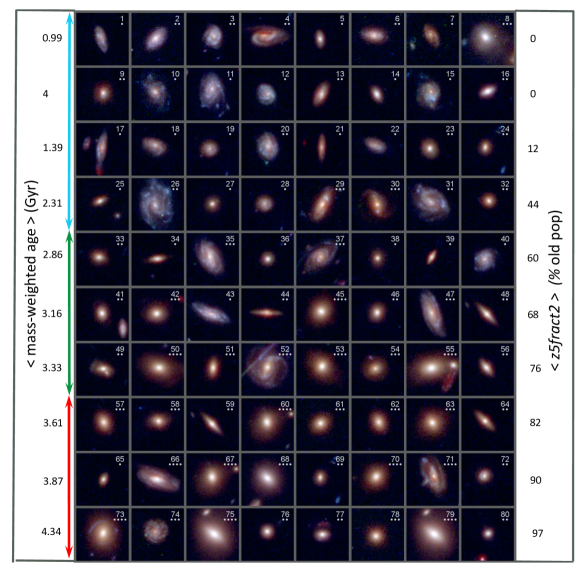
Figure 4.— CANDELS HST images for high-confidence SFHs from this study. 80 observations of 74 galaxies with 6 repeat SED measurements (see Figure 5 and Table 1). Images (identical for repeats) are arranged by increasing z5fract2, as is indicated by the mean value of z5fract2 (right column) for each row, expressed as the percentage of old stellar population (rather than a fraction). Images are RBG, created from F606, F814, F160 images from WFC3; each box has a physical scale of $\sim$35 kpc on a side. The number in the upper right corner of each image is the catalog number in Table 1. The dots below the catalog number give the measured stellar mass for each observation binned by factors-of-two: $\log M_{\ast}=10.0$–10.3 (one dot), 10.3–10.6 (two dots), 10.6–10.9 (three dots), 10.9–11.2 (4 dots). The mass-weighted age in Gyr (not to be confused with commonly used light-weighted agefrom the vantage point of T_obs, averaged over each row, is given in the left column. Three ranges of SFH fits are indicated: (blue arrow) late bloomers—95% confidence $<$50% old population ; (green arrow) old, approximately constant star formation—95% confidence $>$50% old population; (red arrow) old—95% confidence $>$70% old population. The duplicate IDs—19/28, 24/69, 48/59, 57/62, 60/67, 75/79—show that SFHs place both members of the pair in the same category—late bloomer, constant star forming, old galaxies.

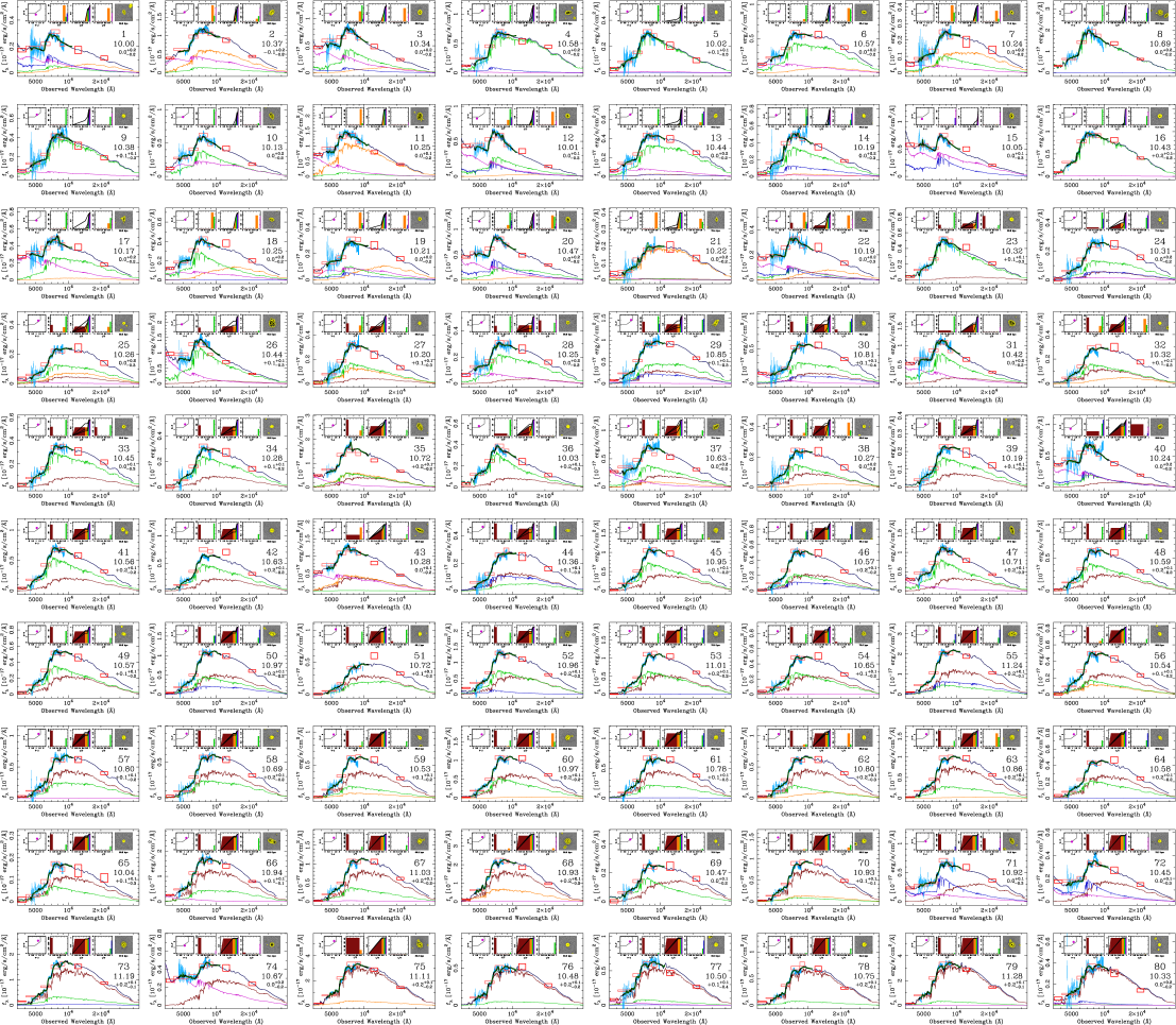
Figure 5.— SEDs for Galaxies with HST images and high-confidence SFHs from this study. Documentation on how to read these SED plots is given in Figure 2. The SEDs are arranged to match the images in Figure 4 and are include the image/catalog number for convenience.

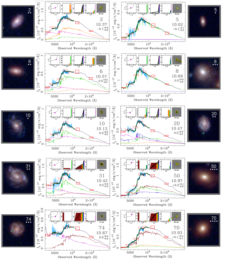
Figure 6.— Images and SEDs for 10 galaxies with high-confidence SFHs from this study, showing the range of histories and morphologies of galaxies, from old galaxies to late bloomers. The top three rows are for late bloomers: each galaxy has a contribution from an old population (earlier than T_obs–2 Gyr) of less than 50%, at the 95% confidence level. IDs 5 and 8 appear to have “early type” morphologies and a single stellar population of age 0.5–1.0 Gyr that well fits the SED, as discussed in the text. It is worth noting that, in the UVJ diagram (top left box), three of the six late bloomers are clearly situated in the “passive” area, showing that this diagnostic is indicative of the most recent epoch of star formation rather than a more general indicator of long term star formation or passivity. The galaxies in the bottom two rows have old populations of more than 50% at the 95% confidence level. The CSI SFHs for IDs 31 and 50 are more-or-less constant in time (a diagonal line in the mass growth plot) while 74 and 70 have are dominated by old stars ($>$70%) with contributions of $<$10% of stars born within 2 Gyr of T_obs. With respect to morphology, IDs 50 and 70 are early types, while ID 31 is clearly a spiral disk galaxy. ID 74 shows a spiral pattern, but this is apparently due to a small fraction of stellar mass in a starforming disk, in an otherwise spheroidal, old galaxy.

Figure 4 is a mosaic of the 80 HST images of the 74 catalog objects. Figure 5 shows the corresponding SEDs for each observation as described below. Table 1 identifies these objects by RA and DEC and provides basic data for each of the 80 observations: $i$-band magnitude; prism spectrum $S/N$; $z$ (1$\sigma$ errors); $\log M_{\ast}$ (5%–95% confidence interval); fractional mass-growth history (1$\sigma$ errors) at 2 Gyr (i.e., z5fract2), 1 Gyr (i.e., z5fract), 500 Myr, and 200 Myr before T_obs; and n2, local galaxy number density in Mpc^-3 derived from the full CSI catalog ($r=2$ comoving Mpc aperture).

Figure 4 is arranged by increasing z5fract2: late bloomers are on top with the oldest galaxies at the bottom. The sample is not strictly speaking a random draw from the 128 possibilities because it is biased to more-certain SFHs and to late bloomers, which make up 40% of the galaxies in this “gold sample,” compared to 20%–30% of observed galaxies overall (see Section 3, Figure 3. The numbers to the right of each row give its $\langle{\it z5fract2}\rangle$ as a percentage, with mean mass-weighted-ages on the left. All quantities are derived from the SFHs/SEDs of Figure 5.

As the appendix explains, based on simulations, the z5fract2 values for the late bloomers in Figure 4 can be treated as lower limits: the 0% in the first two rows reflects non-detections of a population that may be as high as 60%. However, the simulations also suggest that the late bloomer sample in these figures/tables is about 75% pure, and that a majority of the 25% contaminants that formally breach the ${\it z5fract2}<0.5$ bound have, in reality, $0.5<{\it z5fract2}<0.6$. These are still very young galaxies, considering that this is the fraction of mass produced in the first $\sim$5 Gyr compared that made in just the 2 Gyr before T_obs. In any event, future investigations using better data with higher resultant purity ($P\gg 0.75$) in their SFH classifications should concur on about $3/4$ of our late bloomer classifications (see Section 2.4). We encourage such new observations but are open to sharing our own data for use in novel, improved analyses.

4.1. Morphology and Galaxy Age

Figure 4 is divided into three sections: 4 rows of late bloomers (the blue range), 3 rows of more-or-less constant star formation (the green range), and 3 rows of the oldest galaxies (the red range). The main bias of the 74 galaxy catalog with respect to a random draw of the full CSI SWIRE catalog is only an over-representation of late bloomers at the $\sim 30$% level. Therefore, we can use this subsample to make two remarkable assertions about galaxy evolution. The CANDELS images in Figure 4 tell us that

1. Massive galaxies, $M_{\ast}>10^{10}$ M_⊙, come in a range of ages, including those that formed all their stars early in the universe, those that formed them over a long time, but also late bloomers, which formed most of their stars after the universe was already 6 Gyr old. There is a trend with mass in the sense that less massive galaxies are generally younger, but as we have found many times in studies of galaxy evolution, all types are represented at all masses, with differences only in the mean;

2. Galaxies of all ages come in all morphologies. There is a trend in Figure 4 that younger galaxies are generally more disky and the oldest galaxies are more likely to be spheroidal, but again, for each class, all morphological types are represented: only the mean type changes.

The first point above is made even in the first row of galaxies, for which no old population is detected: three have masses close to 10¹⁰ M_⊙ (IDs 1, 5, 7), and one galaxy is more massive than the Milky Way (8). Of the 7 different galaxies in the bottom row—almost entirely old stellar populations—three have masses of $\sim$2 $\times$ 10¹⁰ M_⊙ while 2 exceed 10¹¹ M_⊙. In a similar vein, disk galaxies with large, presumably massive bulges are found all over the mosaic, for example, IDs 2, 8, and 23 among the late bloomers and 53, 60, and 75 among many of the old galaxies. Likewise, small bulge galaxies are probably expected for late bloomers—for example, 1, 15, and 22—but they are found all the way down the age sequence, for example, 43, 52, 66, 74.

The point is that galaxies encompass SFHs that are very fast, very slow, or very late in a way that is correlated to mass and morphology, but not in a strong way. Simple models that predict the appearances of galaxies, old to young, tell only part of the story.

4.2. Ten Examples of Late Bloomers and Their Elders: Images and SFHs

Figure 6 provides images and SEDs for 10 galaxies: 6 late bloomers and 4 old, 2 of which are have long-term, continuing star formation. Along with the two SEDs of Figure 2 and its discussion in Section 2, this figure will help the reader interpret the compendium of 80 SEDs for the 74 cataloged galaxies in Figure 5.

Among the 6 selected late bloomers, we see a variety of SFHs, but all developed after $z\approx 1$, and for each the envelope of “allowed” SFHs is very narrow. By definition, none have a detected old stellar mass fraction of $>$ 50% as an upper limit, but in these 6 examples, even within the 95% confidence interval, there is no evidence for a stellar population that formed earlier than T_obs – 2 Gyr (the brown rectangle is not present). However, we reemphasize that this does not preclude the presence of a sizeable old population: our sensitivity to $<$10¹⁰ M_⊙ is borderline, and less than 3 $\times$10⁹ M_⊙ in old stars is very unlikely to be detected, as the discussion in the appendix explains. All 6 late bloomers show considerable star formation in the 1–2 Gyr and 0.5–1.0 Gyr populations (orange and green) or both, suggesting that these are galaxies with a several-Gyr history of star formation, as opposed to a few-hundred Myr burst. One late bloomer is passive at T_obs and—of the five that are starforming—SFRs have mainly declined in the last 0.5 Gyr. All are dusty, with measurable, sometimes large extinction at all ages $<$2 Gyr. Four of the 6 are disk galaxies (for the four rows of late bloomers in Figure 4, 17 of 24 are), and all of these have small-to-moderate bulges.

The most striking feature of this group of late bloomers comes from IDs 5 and 8, both massive galaxies that would, by appearance, normally be considered early types. These appear to be entirely composed of A stars (the green 0.5–1.0 Gyr population). Only a single young stellar template is required for a very good SED fit. This suggests a remarkable SFH, to be sure, but perhaps more remarkable is the amount of stellar mass involved: $\sim$10¹¹ M_⊙ of gas was turned into stars in approximately 1 Gyr. (An all-green SFH solution is likely consistent with star formation over $\sim$2 Gyr, whose mean age is that of the green age bin, but this is hardly less surprising.) As we saw in the statistical sample discussed in Section 3, if these massive, spheroidal galaxies with a sudden stellar buildup after $z\approx 1$ are not common, neither are they rare. Based on this small sample, 3 others—a total of 5 of the 24 late-bloomers in Figure 4—appear to have the same morphology and whiter “color” that distinguish them as a different kind of system from the redder images of spheroidal galaxies identified as truly old, visual evidence that these are a different kind of system.

In summary, not only is it remarkable that there are massive galaxies that make most of their stars around $z\sim 0.8$, but moreover, some of these have the the “early” morphology associated with old, massive galaxies, and certainly not associated with a large amount of young stars. “Late bloomers” already land in the “unexpected” category, we think, but arriving in many morphological types adds to a puzzle, which must be solved—if understanding galaxy evolution is the goal.

For IDs 50 and 74, the two examples of more-or-less-constant star formation, the presence of multiple epochs of star formation is the common feature of this type. Of the two, one is very actively forming stars but the other is not—it appears to be an old galaxy (and old looking, too) that had a MWs mass of gas dumped on it in the last Gyr or so, which it promptly turned into stars. “Accretion” seems more than an understatement, but neither does this resemble a major merger, given the large gas fraction required.

The two very old galaxies in the bottom row are more than 95% old, but each shows signs of a small amount of late star formation—a late “frosting,” and a heavy one at that. For galaxy 74 the star formation is ongoing and a prominent spiral pattern is seen, but it seems likely that the bulk of the stellar mass is spheroidally distributed, with a thin disk hosting the brief return to life of this galaxy. Galaxy 70 is an example of what we would likely call, looking back from the present epoch, a completely old galaxy, suggesting that late episodes of significant star formation 5–6 Gyr ago were common for these as well (see also, e.g., Treu et al. 2005). Neither of these galaxies will have been passive for all of its life up to “today”—i.e., they will have left the quiescent region of the UVJ diagram after initially entering it—something that deserves more investigation with larger samples that include morphologies.

5. Discussion

In this section, we begin with a phenomenological description of late bloomers in the broader context of what is known about the evolution of MW-like galaxies. We then ask how late bloomers fit into the dark matter halo/$\Lambda$CDM picture via a comparison to a semi-analytic model. This is only a short introduction to what could be a complex and broad-reaching challenge: What aspects of the widely accepted picture of halo and stellar mass growth—and the agents of abatement that lead to a “cosmic winter” of galaxy building—are actually physically illuminating.

5.1. Late Bloomers: What, When, Where, How, and Why?

For newly recognized phenomena, these simple interrogatives define a traditional first step towards understanding. In this section, we review the state of the subject of late bloomer galaxies as we now see it.

5.1.1 “What?”

The “what” of late bloomers rests on the reliable determination of SFHs that are not part of the canon—i.e., do not correspond to those generated by integrating scaling laws such as the SFMS. The direct implication is that a significant fraction of presently MW-mass (and probably greater) galaxies experienced most of their star formation in the “cosmic autumn” instead of “cosmic spring” or “summer,” something that has not been recognized from studies of present-epoch galaxies (though cf. Marínez-García et al. 2017). From a theoretical perspective, late bloomers might be outside expectations if their growth in stellar mass departed substantially from the growth of their dark matter halos, as judged from, e.g., $\Lambda$CDM $N$-body simulations. In this context, late bloomers could be galaxies whose SFHs are delayed with respect to their dark matter halo growth. Section 5.2 discusses the above questions in more detail.

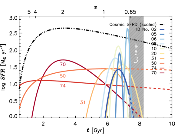
Figure 7.— Lognormal SFH fits for the 10 galaxies in Figure 6. The dot-dashed black line is the cosmic SFR density. The six late bloomers (blue-to-green lines) have the form that is unique to a two-parameter SFH model (like the lognormal). They peak at late times, after $z=1$, but form their considerable stellar masses in 1–2 Gyr, in stark constrast to the SFRD and the SFHs of old galaxies. Two of the 4 old galaxies in Figure 6, IDs 70 and 74, peak early—near or before the SFRD peaks. ID 74 appears in its lognormal parameterization to have a very extended history of star formation, but this is probably an artifact of significant star formation at T_obs; such bimodal SFHs are poorly described by a lognormal. ID 50 is an example of a galaxy whose SFH is approximately constant. ID 31 appears to rise well after the SFRD peak, but its star formation history is broad and might have been called a late bloomer if observed 1-2 Gyr earlier.

5.1.2 “When?”

The “when” of late bloomers is best approached by finding a way of characterizing their exceptional SFHs. Our parameterization of SFHs as lognormals is such an approach. While lognormal SFHs may be an approximation and subject to alteration by late processes like galaxy mergers and baryon accretion, the success of this model in reproducing the “bulk properties” of galaxies demonstrates its suitability as a starting point (G13, A16).

In Figure 7 we show fits to lognormal SFHs for the 10 galaxies of Figure 6, obtained by solving for the $(T_{0},\tau)$ pairs that best reproduces each systems’ total mass at the end of the five CSI SFH bins. The two old galaxies, 74 and 70, show small $T_{0}$ but long $\tau$, not far from a traditional exponential model (Tinsley 1972). Our measurements are upper limits—$T_{0}$ could be earlier and $\tau$ shorter—since our ability to age-date loses sensitivity before the peak in the SFRD at $z\sim 2$. We are on firmer ground in the case of more-or-less-constant star formation, ID 50, whose timescales are within our effective time horizon.

The SFHs that are best captured by a lognormal parameterization are the 6 late bloomers (and perhaps one marginal case, ID 31): these are well constrained by the best-measured star formation rates, $\mathrel{\raise 1.50696pt\hbox{$\scriptstyle<$}\kern-6.00006pt\lower 1.72218pt\hbox{{$\scriptstyle\sim$}}}$2 Gyr old populations, and the minimal to less-than-equal contribution from an old population. Thus, at these stellar masses, the long $T_{0}$, short $\tau$ values for late bloomers are the distinguishing features of this type (see Figure 4), a combination of values that may or may not be consistent with a conformal galaxy growth model.

We know, from the adequacy of simple declining exponential models to fit the the SFHs of local galaxies, that late bloomers are essentially extinct today, at least for galaxies more massive than 10¹⁰ M_⊙. By this we mean that, if measurements are made for $z\approx 0$ galaxies to focus on star formation that occurred since 2 Gyr before the present epoch ($z\approx 0.16$), there should be no late bloomers; i.e., no galaxies with a substantial fraction of the stellar mass formed during that period. The decline of the late bloomer population from $\sim$20% at $z\sim 0.8$ to near zero today was first documented in O13 and confirmed in the D16 study. Figure 8 shows this result from the CSI sample for this study. At $z=0.7,0.6,0.5,0.4,0.3$, the LBF noticeably declines from $\sim$30% to $<$5% at the MW’s current mass of $\log M_{\ast}\sim 10.7$.

Note that the LBF at $\log M_{\ast}\sim 10.2$ and $z\sim 0.7$ is about twice that at $z\sim 0.4$ (2 Gyr later) for $\log M_{\ast}\sim 10.6$ . Hence, a meaningful fraction of late bloomers will go on to double once more over the course of their lives, growing 0.6 dex in 4 Gyr.

It is worth distinguishing this signal from the very different question of whether we could recognize that a present-epoch galaxy was a late bloomer at $z\sim 0.6$ (i.e., was a descendant of one of the CSI systems). That answer is probably no: with present techniques based on integrated stellar populations, it would be very difficult to recognize that a $z\sim 0$ galaxy had its major star formation 6 Gyr ago rather than 8+ Gyr ago. For this reason—and the near-zero $z\approx 0$ LBF—we should not be surprised that there has been no hint of late bloomer SFHs from studies of present-epoch galaxies.

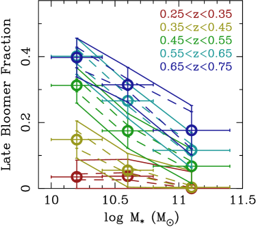
Figure 8.— The dependence of the late bloomer fraction (LBF) on mass and redshift. The LBF declines with increasing mass but also with decreasing redshift: later than $z\sim 0.3$, late bloomers effectively disappear at $\log M_{\ast}>10$.

Are there late bloomers at higher redshift, $z\mathrel{\raise 1.50696pt\hbox{$\scriptstyle>$}\kern-6.00006pt\lower 1.72218pt\hbox{{$\scriptstyle\sim$}}}1.0$, for example? G13’s original lognormal realization suggests that short $\tau$ SFHs spread from the earliest times (starting with old galaxies like IDs 74 and 70) through the SFRD peak, all the way to $z\sim 0.3$, but disappear at lower redshifts (consistent with Figure 8. In principle, CSI data at $z\mathrel{\raise 1.50696pt\hbox{$\scriptstyle>$}\kern-6.00006pt\lower 1.72218pt\hbox{{$\scriptstyle\sim$}}}1$ should be able test this, but beyond $z>1.2$, our data will not be able to answer this question: The break region redshifts out of the optical, and in any case we imagine that the shorter age of the universe would make it very difficult to distinguish long $\tau$ from short $\tau$ for galaxies with $T_{0}$ approximately that of the peak in cosmic star formation. The takeaway is that massive late bloomers probably cover the whole of cosmic history up to a few Gyr ago, even if, operationally, they are hard to distinguish as a separate class of objects at $z\gtrsim 1$.

5.1.3 Where?

Figure 9, left, shows the distribution of galaxy overdensities around secure late bloomers (LBs) and non-late bloomers (NLBs) for the full CSI sample, measured in 1 Mpc apertures. From this perspective the “environments” of LBs appear similar to those of NLBs, with mean densities differing by only $\sim$25%. Figure 9, right, shows the correlation of mean local galaxy density with the scales over which they are measured; NLBs live in regions with slightly higher density on scales at least to 8 projected comoving Mpc.

Some part of this signal is due to the fact that the galaxies least likely to be late bloomers—elliptical galaxies and other passively evolving systems—are known to live in the densest regions (Dressler 1980) and are the most strongly clustered (Davis & Geller 1976, Loveday et al. 1995). We can remove this signal by eliminating all galaxies in the upper quartile in projected galaxy density ($\Sigma_{\rm 1\,Mpc}$, orange dashed line). Figure 10 presents the results.

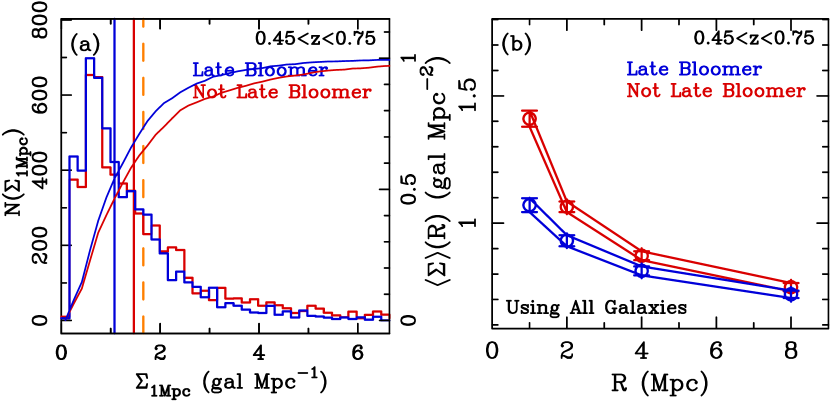
Figure 9.— (a) (thick lines) Distributions of local projected galaxy densities within projected radii of 1 comoving Mpc and $\Delta z\pm 0.02(1+z)$ around late bloomers and non late bloomers. Cumulative distributions are shown using the thin lines. Orange vertical line marks the 75th percentile of the full distribution of galaxy densities. Mean local densities for late bloomers and non-late bloomers are shown by the blue and red vertical lines, respectively. (b) Mean local projected galaxy densities around late bloomers and non-late bloomers as a function of project scale over which densities are measured.

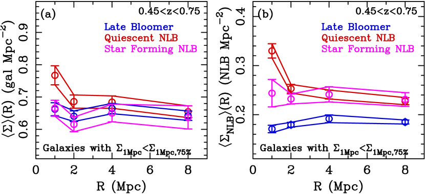
Figure 10.— (a) Mean local projected galaxy densities around those late bloomers and non-late bloomers with $\Sigma_{\rm 1\,Mpc}$ less than the 75th percentile (orange line in Figure 9) as a function of project scale over which densities are measured. Late bloomers and non-late bloomers live in neighborhoods with similar numbers of neighbors. (b) Measuring densities of non-late bloomer neighbors, we see that late bloomers prefer not to livearound non-late bloomers, and that non-late bloomers prefer to live around each other. This homophily of galaxy SFHs either reflects long-term exposure to similar environmental forces, or different sets of initial conditions that set ensembles on paths to beingearly or late forming.

The remaining LBs now appear to inhabit almost exactly the same environments as ordinary, starforming galaxies (see blue and violet lines in Figure 10a). One might therefore conclude that, in the general field, LBs do not live in particularly interesting places. However, this is not the case: When one measures environments by counting only the NLB galaxies—the systems generally thought of as “normal,” with SFHs that began their decline at $z\gtrsim 1$—a very different signal emerges.

Figure 10b shows that late bloomers avoid non-late bloomers. Although, projected on the sky, LBs do not live in regions specially marked as over- or under-dense in all galaxies, late-growing galaxies nevertheless do live in special places: ones with markedly fewer NLBs (starforming or not).

Two implications stem from this finding. One is simply (again) that LBs are a real phenomenon, not some noise-selected subset of the normal galaxy population.

The second is more profound: galaxy SFHs trace environmental histories. Moreover, since z5fract2 depends on the SFR averaged over the first $>$4 Gyr-wide bin, they do so over long timescales. Though they may have just as many neighbors, late bloomers do not grow up in non-late bloomer neighborhoods; those neighborhoods apparently do not foster, and have never fostered, LB behavior (see also O13).

In sociology, “homophily” is the tendency of individuals to form relationships with other, similar individuals. In astronomy, “red galaxies cluster” is an example of homophily. Here, however, we are encountering homophily not as a function of present attributes, but historical ones. The signal in Figure 10b suggests that galaxy childhood and/or inheritance matters: Either star formation behavior and performance over Hubble timescales reflects (1) prolonged childhood exposure to similar environmental factors, or (2) accumulated biases towards early or late growth inherited from initial conditions (e.g., KBA2016). We cannot yet say, specifically, what these factors/biases are, but they would seem to be poorly encoded by the overdensities inhabited at T_obs (e.g., Mo & White 1996). Halo mass at T_obs must also be a poor proxy under either scenario, outside of the most clustered halos hosting the most quiescent NLBs. Only once you have the SFHs can you tease out these key facts.

5.1.4 “How?”

“How” can be approached in many ways, but we think the heart of the question is this: How can major star formation in $\sim$one-fifth of massive galaxies be postponed by billions of years compared to their peers?

The obvious appeal is to major mergers, but two arguments push back on this possibility. First, as established by a number of studies using a variety of techniques (e.g., Bell et al. 2006; Williams et al. 2011; Man et al. 2016) the major merger fraction at these epochs is only about 6%, less than $1/3$ of the CSI LBF estimate. Second, such mergers would have to be extremely gas rich/entail systems with quite low $M_{\ast}/M_{\rm halo}$. Recall: our SEDs and SFH inferences are sensitive to the mass present before the late bloomer “episode.” Hence, to explain MW-mass late bloomers in which little or no old stellar mass is detected (not atypical; see Figure 4), two $\sim 10^{12}\,\rm{\hbox{$\,$M${}_{\odot}$}}$ halos that are mostly gaseous would have to merge. Given that effectively all results from abundance matching show such haloes having, on average, the highest stellar mass fractions (e.g., Moster et al. 2013; Behroozi et al. 2013a), this scenario seems highly unlikely. Assuming an 0.2 dex scatter in $M_{\ast}/M_{\rm halo}$ (Behroozi et al. 2013b), and that the MW’s $M_{\ast}\sim 10^{10.7}\,\rm{\hbox{$\,$M${}_{\odot}$}}$ is representative, our $M_{\ast}\sim 10^{10}\,\rm{\hbox{$\,$M${}_{\odot}$}}$ detection threshold corresponds to a more-than-3 $\sigma$ low-side outlier for a given halo mass, far too rare to account for the late bloomers.

While it is true that dark matter halos show a range of collapse times—the result of a spread of initial densities at a fixed mass—a doubling of collapse times for a fraction of $\sim$20% of $\sim$10¹² M_⊙ halos may not comport with current $\Lambda$CDM simulations (see Section 5.2). If not, baryonic physics is the only plausible agent. Indeed, the importance of “feedback” in modeling galaxy evolution has grown rapidly in this decade, particularly as a feature needed by the simulations to retard or stop the growth of massive galaxies (to match the observed mass function) when plenty of gas remains to fuel star formation. By expelling gas into a galaxy’s halo, winds driven by vigorous star formation and/or supernovae, or powered by AGN outbursts fed by gas inflow, could suppress star formation—temporarily or permanently.

The problem of invoking feedback to explain late bloomers is that such influences are least expected here. Late bloomers have formed a smaller fraction of stars for their halo mass, so feedback from star formation is minimized, and galaxies that have had little stellar mass growth are not good candidates for large supermassive black holes. This does raise an interesting and answerable question: what is the incidence of Seyfert nuclei in late bloomers compared to “normal” populations? Again, the most remarkable feature of this phenomenon is that, with $\mathrel{\raise 1.50696pt\hbox{$\scriptstyle<$}\kern-6.00006pt\lower 1.72218pt\hbox{{$\scriptstyle\sim$}}}$10¹⁰  M_⊙ of mass in old stars, how do these systems retain $10^{10}\mathrel{\raise 1.50696pt\hbox{$\scriptstyle<$}\kern-6.00006pt\lower 1.72218pt\hbox{{$\scriptstyle\sim$}}}M_{\rm gas}\mathrel{\raise 1.50696pt\hbox{$\scriptstyle<$}\kern-6.00006pt\lower 1.72218pt\hbox{{$\scriptstyle\sim$}}}10^{11}$ M_⊙ of gas to $z\sim 1$, some 6 Gyr after the big bang, and then begin to form stars at furious rates of 10–100  M_⊙ yr^-1, long after their elders passed through that phase. How, indeed?

5.1.5 “Why?”

At the heart of the “why” of late bloomers, we think, is the fundamental question of what processes shape the SFHs of galaxies—all galaxies. The reigning paradigm has been “grow and quench,” the idea that stellar mass grows along global scaling laws, such as the SFMS, until some feedback mechanism sharply curtails star formation, or ends it altogether. The picture is widely accepted, even in the absence of a uniquely successful model for the quenching mechanism. Furthermore, ensemble properties of galaxies—for example, mass functions and fractions of active versus passive galaxies—provide very weak constraints, easily satisfied by very different models (A16; KBA16). Sufficient numbers of individual examples of galaxies in the act of quenching are not identified, and models and predictions of what observations might be discriminating are not offered.

Quenching, to be meaningful, is by definition a short timescale process that requires an event that alters the course a galaxy would otherwise take. There is scant evidence for this at low redshift. Most SDSS “green valley” galaxies are not recently-quenched galaxies from the “blue cloud,” as had been suggested (e.g. Faber et al. 2007): expected UV color evolution and spectral features (strong Balmer absorption without star formation) is seen in only a few percent of the population (Schawinski et al. 2014; Dressler & Abramson 2015; Rowlands et al. 2018). In fact, green valley galaxies are evolving slowly towards the red sequence, as star formation slowly ebbs. Acknowledgement of this fact has led to the introduction of an oxymoronic “slow quenching” to describe what is certainly better characterized as galaxy evolution over a Hubble time.

Perhaps, as originally suggested, massive galaxies at high redshift truly quench—rapidly—but a “smoking gun” requires the identification of a mechanism and its observation. An appropriate alternative is one that invokes Hubble-timescale processes—which, by definition, become rapid at high-$z$—to shape the SFHs of all galaxies, like the lognormal model we have developed (G13, D16, A16). As with quenching, the success of this model has been largely judged by its ability to reproduce the mean properties of galaxy populations through cosmic time. However, as we have shifted our focus to the SFHs of individual galaxies (D16 and this paper), we believe that this richer data set moves the discussion from “why do galaxies quench?” to “why do galaxies follow a Hubble-time-scale form?” (See also Pacifici et al. 2016.) For both rapid and slow forming galaxies we see a common theme: galaxies grow as long as their gas fractions are high and fall as stellar mass overtakes available gas for further star formation. However, the critical physics that translates this observation into a lognormal or similar SFH remains elusive.

We suggest that late bloomers are key to understanding what shapes star formation histories because they are simply non-existent within grow and quench scaling law-driven pictures, but they are clearly real. The “why” of late bloomers is, then, their role in properly and fully describing the histories of star formation for all galaxies. Any model that does not produce late bloomers must be incomplete, but models in that category should view late bloomers as an opportunity to learn about and/or tune the physical inputs to their star formation prescriptions. What is clear is that late bloomers are a new, potentially strong constraint on future simulations and theory of galaxy growth.

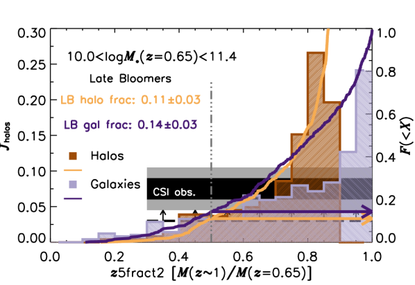
Figure 11.— Theoretical halo (orange) and galaxy (purple) z5fract2 values (left axis) and LBFs (right axis) based on the GALACTICUS semi-analytic model. Orange and purple horizontal arrows highlight the halo and galaxy model LBFs, respectively, while the black/gray solid horizontal bands show the CSI empirical results (see Figure 3). Only model halos harboring galaxies above the CSI completeness limit in the empirical analysis—$\log M_{\ast}\geq 10$—are considered. Binomial uncertainties show the 95% model confidence interval. GALACTICUS’ halo LBF is consistent with the empirical lower-limit: its galaxy LBF with the best observational estimate at $\sim$1 $\sigma$.

5.2. Late Bloomers, Dark Matter Halos, and the Grow and Quench Paradigm

In this section, we consider the late bloomers we have found at $\sim$20% abundance in our $z\sim 0.6$ sample in the context of a semi-analytic model of galaxy evolution in a $\Lambda$CDM universe. Three issues that stand out are: (1) Are a significant fraction of $\sim$10¹² M_⊙ dark matter halos still assembling at $z\leq 1$? (2) Are theoretical prescriptions used to model baryon evolution able to delay stellar mass growth with respect to halos? (3) What implications do the late bloomers have for established methods of inferring galaxy SFHs from global scaling laws (and quenching prescriptions)? Below, we address these questions in order. Our results are based on the well-tested GALACTICUS semi-analytic model by Benson 2012. They are robust to resolution at least over minimum halo masses of $10^{9}$–$10^{10}\,\rm{\hbox{$\,$M${}_{\odot}$}}$; the .xml input file from which they were derived is appended as an ancillary data file.

5.2.1 “Late” Halo Growth at Milky Way Scales

An obvious question to ask when trying to understand late bloomer galaxies in the $\Lambda$CDM framework is whether a similar number of halos also doubled in mass so rapidly at these redshifts. If so, at least the diversity in halo growth trajectories could encompass that in galaxy SFHs.

To answer this question, we ran GALACTICUS in a “standard” DM+baryons mode (revision 6169:394a64c6b493; see Knebe et al. 2018), tracking 3000 halos. We then selected all 489 halos at $z=0.65$ harboring galaxies with $M_{\ast}\geq 10^{10}\,\rm{\hbox{$\,$M${}_{\odot}$}}$. We identified their most massive progenitor 2 Gyr earlier ($z=1.08$) and defined ${\it z5fract2}_{\rm halo}$ as the ratio of the progenitor to descendant masses. We repeated this calculation for the corresponding galaxies. Figure 11 shows the results.

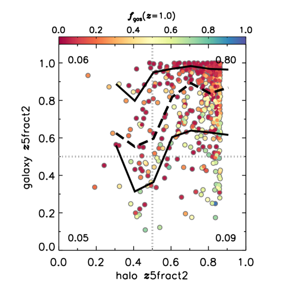
Figure 12.— Halo vs. galaxy z5fract2 from the GALACTICUS SAM. Points are colored by gas fractions—$M_{\rm gas}/(M_{\rm gas}+M_{\ast})$—at T_obs minus 2 Gyr ($z\approx 1$). Dashed/solid black lines show the median/1 $\sigma$ spread, respectively, in bins of 0.1 dex in ${\it z5fract2}_{\rm halo}$. Late blooming galaxies tend to be gas rich, though late blooming halos can host gas-poor galaxies (perhaps suggesting these are not analogous to the actual halos of CSI late bloomers). The fraction of objects is printed in each galaxy–halo (non-)LB quadrant.

The cumulative distributions in that plot reveal that, while most halos only grew $\sim$20% (in agreement with the traditional vision of massive galaxy growth), 8%–15% of those harboring CSI-detectable galaxies did indeed double in mass in the 2 Gyr preceding T_obs (95% confidence). These numbers rise to 11%–17% when examining the simulated galaxies themselves. These fractions are at most a factor of $\sim$2 away from the CSI observations, suggesting that at least the number of halos is sufficient to account for the late bloomer phenomenon, and global baryonic prescriptions are capable of producing them. As such, the existence of these objects was predictable from numerical modeling, though we are unaware of any works that drew attention to them. Certainly, there does not seem to be a compelling reason to rule-out late bloomers from a dark matter assembly perspective (see also Giocoli et al. 2012).

5.2.2 Connecting Galaxy to Halo Growth

Though there may be sufficient late-blooming halos and galaxies in GALACTICUS, the question remains as to the physical connection between these two entities; i.e., is halo assembly sufficient to account for the timing of galaxy growth, or is there something else at play (Section 5.1.4)? Figure 12 plots z5fract2 vs. ${\it z5fract2}_{\rm halo}$ to investigate this link.

While there is a weak trend in the expected sense—late-growing galaxies are more likely to occupy late-growing halos—the scatter evident in this diagram is extreme: galaxies might span 40% in z5fract2 at fixed halo assembly history (to the extent it is encoded by ${\it z5fract2}_{\rm halo}$). As such, baryonic effects are playing a substantial role in late bloomer formation beyond what can be accounted for by the halo histories. This finding echoes results from Diemer et al. (2017; see their Figure 9), though we note no late bloomers were found in that analysis of the ILLUSTRIS hydrodynamical simulation (Vogelsberger et al. 2014), suggesting (perhaps unsurprisingly) that assessing the above baryonic effects will no doubt be sensitive to the specifics of the modeling.

Nevertheless, a clue to the nature of such phenomena that is hopefully so macroscopic as to be insensitive to such details lies in the color coding in Figure 12. This shows galaxy gas fractions, $M_{\rm gas}/(M_{\rm gas}+M_{\ast})$ (an observable, in principle), at $\hbox{\emph{T${}_{\rm obs}$}}-2$ Gyr. Predictably, objects with the highest gas fractions—60%–80%—are much more likely to be late bloomers at fixed halo assembly history than galaxies with the lowest. Indeed, examining the $M_{\ast}$–$M_{\rm halo}$ relationship (not shown) reveals that non-late blooming galaxies in late blooming halos (top-left corner of Figure 12) live in abnormally massive halos for their stellar mass. This suggests they are centrals of assembling groups—i.e., the high environmental density tail we excluded when discussing LB environments in Section 5.1.3. As such, they would typically be passive, consistent with their below-average gas fractions in GALACTICUS. Though substantial scatter persists even here, this kind of statement would represent meaningful input by modelers as to how, where, and why observers might find late bloomers at other epochs or along other axes: if quantitative predictions for, e.g., the mean and scatter in gas temperatures or molecular fractions, local environments, bulge-to-disk ratios, or kinematics were made, these would be testable by future targeted observations or surveys. Other useful inputs include the AGN fraction among late bloomers, their metallicity distributions (stellar and gas-phase), and areas of parameter space that are certainly forbidden under $\Lambda$CDM halo assembly. Correct predictions in any of these veins would go a long way towards reassuring the community that a model captured something fundamental about galaxy evolution that qualitatively distinguished it from others with diverging answers.

5.2.3 Implications for Scaling Law-Based Inferences

Independent of their physical implications, we believe that the late bloomers demonstrate a central, mathematical fact that the community must recognize if we are to gain a meaningful sense of the narrative of galaxy evolution. Simply, late bloomers cannot be described by any model based on abundance matching or the integration of scatter-free scaling laws (e.g., the SFMS). These consequences follow from the fact that late bloomers break mass rank ordering; i.e., though they may occupy the same bin at T_obs as equal-mass systems with constant (or even linearly increasing) SFHs, they were arbitrarily less massive 2 Gyr in the past. As such, they must have jumped over all galaxies in the intervening mass bins to reach the endpoint at which they were identified. If mass—halo or stellar—is taken as the controlling parameter for an object’s growth rate—as it is in abundance matching or SFMS integration—this phenomenon obviously cannot occur.

The implications of this fact could not be more profound: if relative positions on scaling relations do not stay fixed, the above methods become effectively useless for identifying—let alone characterizing—the progenitors or descendants of any galaxy, or even mass-limited sample. Of course, by definition, they are accurate in the mean. However, if, as we find, fully 1-in-5 systems are not only “outliers” here, but contradictory of the methods by which the mean is defined, it is clear not only that the “average galaxy” is unrepresentative of important physics, but that approaching the problem from this vantage point mathematically forbids even the recognition of this fact, to say nothing of illuminating its causes (A16).

This is not to claim that this issue has so far been unknown—Torrey et al. (2017), for example, perform a detailed investigation of the size and character of the effect of mass/abundance rank-order breaking based on numerical simulations. Studies of this kind provide important insights as to where and when galaxies ”jump” each other, and statistical corrections to account for this phenomenon. We encourage further efforts in this vein, but the claim we are making here is that understanding its physical causes/making and testing potentially discriminating theoretical predictions with more global ramifications depends on actually identifying the galaxies that are doing it: late bloomers. Only in this way can we hope not only to learn the amount of SFH diversity, but understand why galaxies take the paths they do through that envelope.

Regardless, the implication from late bloomers on rank-order breaking suggests that further attempts to combine stellar and halo mass functions and SFR scaling laws (of any depth and redshift) will not be edifying. Instead, attention must be paid to inferring appropriately complex SFHs from the SEDs that the above exercises would otherwise have required (Pacifici et al. 2016; KBA16; Iyer & Gawiser 2017; and Abramson et al. 2017 provide steps in this direction).

6. Summary and Future Work

The principle goal of this paper has been to make a compelling case for the reality of late bloomers, massive galaxies that built the majority of their mass at a time when most galaxies were in notable decline. Toward this end, the paper contains five major sections:

• A description of changes made in our spectral fitting program to improve its sensitivity to late bloomers and to provide SFH confidence intervals to assess the likelihood that a galaxy fits that classification;

• The first robust measurement of the late bloomer fraction from individual galaxy SEDs, showing 1-in-5 present-day MW mass systems (more or less depending on epoch and mass) belong to this class. We encourage new, higher-quality observations to verify this finding and are open to sharing our data for novel/improved reanalyses.

• A catalog of galaxies with high-confidence SFHs, images, and basic data that can be used as a standard sample for independent studies by others employing different methods;

• A discussion of the implications of late bloomers in the context of numerical models of structure growth that include prescriptions for star formation, and for popular ideas about galaxy evolution, such as the SFMS, quenching, and abundance matching;

• An appendix with a detailed description of the simulated SFHs to test the sensitivity of our methodology to detecting old stellar populations as a function of $S/N$ and in the presence of dust extinction.

Our conclusion is that late bloomers at redshifts $0.45<z<0.75$ are real and that they represent a significant minority population of galaxies that grew to Milky Way mass and above by the present epoch. The abundance of late bloomers declined rapidly beginning at $z\sim 0.3$ and became extinct (for massive galaxies) by the present epoch. Comparing with theoretical work on galaxy SFHs suggests that a late-assembling population of dark matter halos available to host late bloomers is $\sim$10%, consistent with our lower bound to the fraction of late bloomers, arrived at by assuming that all $\sim$10¹¹  M_⊙ examples are false positives. However, it remains puzzling how such halos would have avoided star formation for $\sim$5 Gyr and reached $z\sim 1$ with enough available gas to fuel the relatively rapid onset of star formation seen in late bloomers.

This idea of a diverse SFHs, including this $\sim$20% fraction that grew late and rapidly, but also declined relatively soon thereafter, is at odds with the prevailing paradigm of an ordered, conformal set of SFHs quenched internally by a mass-related process or externally through environmental agents. Because the paradigm employs the SFMS to infer SFHs and “abundance matching” to relate the growth stellar mass with respect to dark matter halos, this picture has had considerable impact in the study of galaxy evolution—the existence of late bloomers will be important to understanding the limitations of this approach. We have, therefore, devoted most of this paper to examining the basic methods that underlie the discovery of late bloomers, and used synthetic SFHs and simulations to demonstrate that our work is sound. We believe we have made this case sufficiently well that it will be insufficient for others to simply dismiss late bloomers as the result of some unknown difficulty in spectral synthesis, but instead require observations and analyses purposed at testing our results and finding possible mistakes or errors. To support this effort, we have provided a 74-galaxy sample with high-confidence SFHs with basic data and HST images.

Our work suggests several obvious possibilities for future observations that will clarify many of the issues raised in this paper. First, our modeling of late bloomers is built on spectral templates that have higher resolution than the $\sim$30 Å prism spectroscopy used in the CSI study. As such, we can predict with confidence what higher resolution spectra of late bloomers should look like, both for the confirmation of Balmer absorption lines from younger stars and from metal lines from older populations. We are following up the catalog sample presented here with IMACS observations at $\sim$10 Å resolution and expect that others testing our results will likely obtain such improved data.

A second opportunity is investigate the nature of the stochastic component of SFHs as judged by the fraction of late bloomers that are passive at T_obs. This unambiguous observation should yield insights into the duty cycles of episodes of vigorous star formation. This will be especially interesting extended over the redshift range $0.3<z<1.0$ that our CSI data cover well for the kind of analysis we present here.

Finally, towards understanding where late bloomers fit in the context of most galaxies that accomplished the majority of their star formation before $z=1$, it will be important to investigate such properties as AGN incidence, indicators of major mergers or accretion events, and local environment that may hold clues to the late blooming of this remarkable population.

The authors thank the scientists and staff of the Las Campanas Observatories for their dedicated and effective support over the many nights of the CSI Survey. We also thank A. Benson for valuable assistance in running and understanding his numerical model. We especially appreciated Simon Lilly’s fair-minded consideration of late bloomers as examples of physics outside his paradigm of galaxy evolution—this paper was encouraged by his challenge to convince him of the reality of late bloomers. Lastly, we are grateful to the referee for a careful reading and thoughtful report, which asked for additional information that both strengthens our results and should also help readers better understand our methodology and approach.

Appendix A How Many Late Bloomers Are Imposters?

An important goal of this paper has been to compute the global fraction of galaxies that formed at least half their stars between $z=1$ and $z\sim 0.6$. In this appendix we show, quantiatively, how observational noise drives the best-fit solutions away from the intrinsic growth trajectories of the galaxies. We also show how to compensate for such problems without unnecessarily imposing priors on the early growth histories of galaxies, something which could bias the inferred z5fract2 distribution.

A.1. Why Simulations Are Needed To Inform Selection and Statistical Corrections

The principal side effect of observational noise is to diminish one’s ability to detect old stars, especially when the SED is dominated by young(er) stars. For example, if young stars produce 90% of a galaxy’s light, then, at $S/N\lower 1.29167pt\hbox{$\scriptscriptstyle\;\buildrel<\over{\sim}\;$}10$ at a handful of wavelengths, one has virtually no purchase on the old stellar component. This issue is the chief reason why parameterized SFHs are seen by many to be so useful: they bring along prescribed (and proscribed) amounts of stellar mass according to implicit preconceptions of galaxy growth. Obviously, the problems only get worse when young stars produce yet more light, or at earlier cosmic times, when younger galaxies are more common. Inferences about their properties from SEDs will become increasingly dependent on input assumptions about prior growth.

In terms of $S/N$ and information content, we have in CSI independent flux measurements at ${\cal O}(10^{2})$ wavelengths, with most of the data discussed in this paper at $S/N\gg 10$. Theoretically, we retain statiscially meaningful leverage on the old stellar mass in CSI with $\sqrt{N}\sim 10$, even when young stars make up $\sim 90\%$ of the light.

In practice, however, degeneracies arise between dust and the ages of older stars that may lie underneath younger stellar populations: the residual light from such brighter stars might be too noisy to disentangle the effects of reddening from age. Given the complexities of these degeneracies in the data, we must assess their effects through simulations.

More concretely, galaxies that did grow late may have SEDs that appear optimally fit by histories with earlier growth, and vice versa. One strategy, then, would be to identify the metrics by which one identifies as many late bloomers as possible, with the greatest completeness. However, such a strategy may be plagued by many false positives. In particular, the SEDs of galaxies that grew most of their mass early but also had sufficient numbers of young or intermediate age stars, when subject to observational noise, could be falsely identified as late bloomers. A balance must be struck between the purity of the samples identified as late bloomers and its completeness.

We prefer a strategy that minimizes (or at least mitigates against) false positives, even at the expense of inadequately capturing the census of true late bloomers. Obtaining non-zero, but believable, lower bounds on late bloomer fractions already provides strong, negative implications for common approaches to galaxy evolution, for example, the use of mean growth trajectories and abundance matching. Clearly, the identification of a sample that is, say, 95% complete but only 10% pure is not very useful. Ideally, its much mores sensible to construct samples that are simultaneously $>50\%$ complete and $>50\%$ pure. Only through simulations of the data can one hope to verify such procedures.

When certain classes of noisy SEDs may have diminished fractional sensitivity to old stellar mass, one faces two choices for how to proceed:

1. Include strongly constrained early star formation histories as priors in SED fitting, at least for (relatively) early times; or

2. Impose minimal SFH priors and use the broad confidence limits that arise from the increase in noise while maintaining (empirical) ignorance about the underlying nature of (early) growth trajectories.

The former has been an attractive approach in the community, with parameterized SFHs commonly in use to mitigate the larger uncertainties in any weighing of old stellar mass. In order to use maximum likelihood estimates of z5fract2, they must first be derived using priors that adequately reflect the true underlying distribution of growth histories. Unfortunately, inputing what one thinks is the true underlying distribution of growth histories is prone to lead z5fract2 distributions that resemble the starting assumptions. Hence, the appropriate choice of strategy must be (2).

With such an approach, many noisy SEDs may not statistically require the presence of any old stellar mass, but simultaneously the best-fit stellar population parameters ought still be accompanied by increasingly broad confidence intervals for z5fract2. By definition, when the fraction of old stellar mass is increased for such galaxies to levels at which goodness-of-fit metrics depart from optimality, these levels of old mass can be considered as (nearly) “maximum-old-mass” models—as the z5fract2 values are then pushed (nearly) as high as possible without statistically violating the constraints of the data.

We desire simply a census of the number of galaxies in CSI that have no more than half their stellar mass in old stars. Thus, for our application, the true nature of early growth trajectories is unimportant, so long as we can place (strong) upper limits on the old mass present in the galaxies we identify. For example, we are not particularly interested in distinguishing between galaxies that have 10% of their mass in old stars from those that have 20%—they are equally interesting to us cosmologically and astrophysically. Similarly, by first trying only to find galaxies that grew at least half their stellar mass in the last 2 Gyr, one can relegate to a later date the more detailed questions about which grew 70% and which grew 85%, why they did so, and maybe even how.

It is in this context that we now proceed to demonstrate that the best-fit z5fract2 values do not serve our purposes for quantifying how many galaxies grew most of their stellar mass after $z=1$, and that the best way to select late bloomers is to use their 95% upper confidence limits on z5fract2.

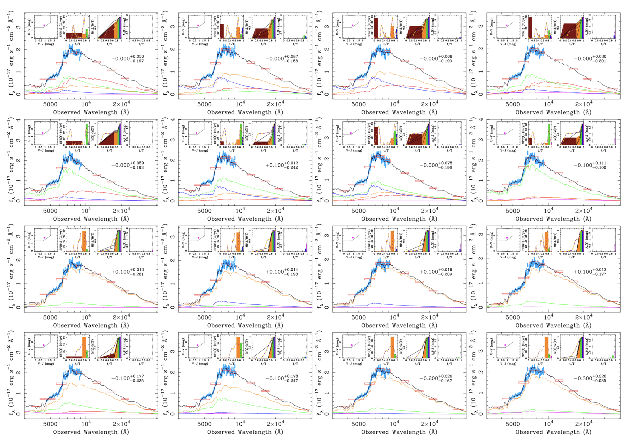
Figure A1.— Rows show example observations for different mock galaxies from Models A (top two rows) and D (bottom two rows) at $S/N=20\,{\rm pix^{-1}}$. The bottom row is for a mock galaxy with half-solar metallicity. Each simulation uses 100 mock galaxies observed 100 times to probe how inferred SFH confidence intervals circumscribe the true SFHs. At this $S/N$, the best-fit SFH solutions (middle two insets) capture many of the features of the underlying true SFH, shown as yellow dashed lines. That our SED fitting generally recovers these basic SFH features is the key result of these simulations. The metal abundances inferred from the SED fitting are listed inside each panel.

A.2. Simulations of CSI Data and their Implications

The ideal set of mock SFHs is one that fills the entire possible empirical parameter space, with a broad diversity of early mass growth independent of later SFRs. By definition, the non-Markovian stochastic SFHs from Kelson (2014), fit the bill perfectly—they are scale-free and have stochastic increments that are zero in the mean. Furthermore, the $1/f$ noise in these SFHs provides a realistic match to the SFMS and its scatter, as well as a diversity of shapes similar to that seen in real galaxies and hydrodynamic simulations (see Kelson 2014; KBA16). Using these as a basis of our simulated CSI data provides a broad range of intrinsic z5fract2 properties and a broad range of ongoing SFRs from quiescence through the vigorous rates of growth seen at intermediate redshift.

The first step was to turn these mock SFHs into SEDs using the Flexible Stellar Population Synthesis models (Conroy, Gunn, & White 2009), fixed (solar) metallicity, $5\leq S/N\leq 80$ for the prism spectra, and variable amounts of dust reddening. In addition to histories generated in a manner consistent with Kelson (2014), we also simulated mock galaxies in which arbitrary amounts of ancient stellar populations were added, allowing for different levels of dust reddening for the old stars compared to that covering the stellar populations that grew over a more extended period of time. The point of this is to vary the amount of old mass that is potentially difficult to detect or even hidden under the noise, contriving situations that bracket what is empirically unknown to help us construct sensible bounds on the fractions of galaxies that grew late.

The simplest runs assume zero dust reddening (Model A), with others having more complexity, such as random screen reddening between $0\leq A_{V}\leq 1$ mag independent of mock galaxy properties (Model B), or random screen reddening up to a maximum $A_{V}$ set by the SFR at T_obs normalized to a maximum of $A_{V}=2$ mag (Model C). Another set solely used histories that have ${\rm SFR}=0$ in their final 30 Myr timestep to help compare sensitivities to z5fract2 in both star-forming and passive mock galaxies (Model D).

The first three simulations (Models A–C) are built on an unbiased random sampling of Kelson (2014) growth trajectories, and therefore have intrinsically high LBFs of 46%, and (apparent) quiescent fractions (QFs) of $\sim 15\%$—derived from inferred sSFR in the last 200 Myr bin (classification by UVJ selection results in a QF of $\sim 17\%$).

Model D has a low intrinsic LBF of 7% because it is comprised of stochastic SFHs with zero ongoing SFR; these histories have a long SFR coherence time. The “observed” 200 Myr sSFRs imply a QF of $\sim 87\%$ (UVJ classification implies a QF of 95%).

We also ran a fifth model—Model E—identical to Model B except in that 25% of the mass is added as very old stars hidden with $A_{V}=2$  mag. This test probes the extent to which old stellar mass that only modestly impacts galaxy SEDs may bias measurements of the early mass fractions. It has a a similarly low QF to Model B, despite the significantly lower intrinsic LBF.

These simulations test sensitivity to the relative amounts of old stellar mass at a range of $S/N$ and broad levels of dust reddening. In such models the old stellar populations may be more attenuated than is realistic, though as starforming disk galaxies are seen edge on, the effects of dust reddening on integrated colors can be significant (Patel et al. 2012). Having greater amounts of dust mixed with the old stars than is present in the starforming disks, however, is an infrequent occurance, even though our stellar population fitting certainly can model such mixtures.

Figure A1 shows examples of such mock SED observations in a manner similar to the presentation of CSI data in Figure 5. Qualitatively, late-time mass fractions are generally consistent with the true values from the input SFHs. Table 2 summarizes CSI’s ability to quantitatively select galaxies that grew more than half their stars in the 2 Gyr prior to observation from the five sets of simulations. For each set we provide the “observed” quiescent fractions (again using the 200 Myr age bin from the best-fit SED), as well as the intrinsic LBF of the set, followed by the measured LBFs using selection of LBs by ${\it z5fract2}_{ML}<0.5$ and ${\it z5fract2}_{95\%}<0.5$. Both reddening and noise change the ability to detect/identify late bloomers quantitatively but not qualitatively. Serious degradation in the ability to reliably identify late bloomers occurs once the $S/N\lower 1.29167pt\hbox{$\scriptscriptstyle\;\buildrel<\over{\sim}\;$}10$ per pixel, for reasons already elucidated.

A.2.1 The Four Questions

Having run hundreds of SFHs at many $S/N$, $A_{V}$, etc., according to the above schemes, we can now answer The Four Questions:

1. What metrics can be used to robustly measure the late bloomer fraction?

2. How accurate are the observed late bloomer fractions?

3. How pure is the late bloomer selection?

4. What are the chief contaminants in an observationally selected late bloomer sample?

Metrics for Measurement of LBF

Selecting late bloomers using ${\it z5fract2}_{ML}$—the maximum likelihood z5fract2 estimates—always over-estimates what (and which) fraction of the population grew most of their mass in the last 2 Gyr. Too many galaxies that did not grow so late have best-fit SED parameters that identify too little early stellar mass due to noise in the data and the way it reduces the statistical significance of pixels that deviate from the fit by young and intermediate-aged stellar populations. Thus, there is too little information present for the best-fit solutions to encode sufficient amounts of old stars.

A more probabilistic approach, whereby the 95% upper limit is used to select late bloomers with a threshold of ${\it z5fract2}_{95\%}<0.5$, yields significantly more accurate LBFs, with significantly improved purities. Answer No. 1 is thus: When there are late bloomers, we can count them most robustly using a selection of ${\it z5fract2}_{95\%}<0.5$.

LBF Measurement Accuracy

While the measurements of late bloomer Fractions using the Maximum Likelihood selection are always too high, the selection by 95% upper confidence limits appears not to overestimate the LBF by more than a few percent. The presence of dust appears to diminish the ability to classify $\sim$10% of galaxies, for which the noise and resulting covariances/degeneracies between reddening and old stellar mass simply produces confidence intervals that are too broad for robust late bloomer identification, even if their ${\it z5fract2}_{ML}$ values would have led to inclusion. We would much rather lose late bloomers and underestimate the true LBF if it means strengthening the empirical evidence for this populations that challenges “established” concepts and approaches such as the preservation of mass rank-ordering. Answer No. 2 is thus: Our measured late bloomer Fractions appear only to require small corrections. In detail, we estimate corrections for the quiescent and star-forming fractions of galaxies separately, thus creating a weighted correction based on the QF in bins of stellar mass and redshift

LB Selection Purity

In parentheses in Table 2 we also list the “purity” of late bloomer samples selected using a given criterion; i.e, ${\it z5fract2}_{ML}<0.5$ or ${\it z5fract2}_{95\%}<0.5$. In the models that most closely mimic the actual CSI sample—Models A–C—these numbers are $\sim$75%; i.e., $3/4$ of observational LB identifications should be physically meaningful. Answer No. 3 is thus: Most of the late bloomers that are selected truly grew more than half their mass in the last 2 Gyr. And while we are confident that our selection of individual late bloomers has this level of purity, the question of how many of our catalog entries in Section 4 will be verified by subsequent follow-up, on an object-by-object basis, will follow that of strongly biased coin flips, with results that depend sensitively to the purity with which the follow-up observations can measure the amount of old stellar mass in galaxies dominated by young stellar populations. If follow-up techniques have similar purity to that probed by CSI in this paper, $\sim 75\%$ purity, then these follow-up observations will re-identify only $75\%\times 75\%+25\%\times 25\%$, or $62.5\%$ of our late bloomers as late bloomers. If follow-up techniques can provide an ability to identify late bloomers with $\lower 1.29167pt\hbox{$\scriptscriptstyle\;\buildrel>\over{\sim}\;$}95\%$ purity, then $75\%\times 0.95\%+25\%\times 05\%$, or $70\%$ of the individual galaxies we identified as late bloomers would be reidentified as such. In detail, and as discussed below, we also estimate purities for the quiescent and star-forming fractions of galaxies separately, and create a weighted purity based on the QF in bins of stellar mass and redshift.

Chief LB Contaminants

Importantly, although the purity is never 100%, in almost all cases, the majority of LB false-positives have intrinsic values $0.5\leq{\it z5fract2}\leq 0.6$. Even for mock galaxies observed at the limit of ${\it z5fract2}_{95\%}\sim 0.5$, $\lower 1.29167pt\hbox{$\scriptscriptstyle\;\buildrel<\over{\sim}\;$}75\%$ of these LBs grew more than 40% of their mass in the last 2 Gyr. Answer No. 4 is thus: Integrating over the broad range of possible intrinsic ${\it z5fract2}$ values (which is unknown in a data set), between 50% and 75% of the contaminants have ${\it z5fract2}<0.6$, with half of the remaining contaminants having grown at least a third of their stellar mass in the last 2 Gyr. In other words, almost all of these galaxies are young, even if not late bloomers by our conservative definition. Whether or not such systems are meaningfully distinct from “true” LBs is a topic we encourage other authors to explore.

A.2.2 Corrections to Observed Late Bloomer Fraction by Type

Table 3 dissects the mock observations further, given the modest dependence of LBF accuracy and LB purity on the mix of star-formation activity in Models A–E. Table 3 lists the measured LBFs and purities for mock galaxies classified as star-forming and quiescent (again using their 200 Myr sSFRs). In principle, the statistics in Table 3 can be used to construct corrections to any measured LBFs if one takes into account the mix of quiescent and star-forming galaxies in a given sample.

For example, at intermediate redshifts in CSI, $\sim$70% of galaxies at $\log M_{\ast}>10.8$ are quiescent. For such galaxies, the models indicate we should observe an LBF of $\sim$0.05, with approximately zero systematic error. For the $\sim$30% of galaxies in that mass range that are star-forming, perhaps they are similar to the galaxies classified as star-forming in Model D, only that there are a few more of them (to lower the apparent QF from 87% to 70%). Table 3 suggests that we would observe an LBF of $\sim$0.39 for the star-forming ensemble, even though the intrinsic LBF may be lower by $\sim 0.07$.

These estimates of systematic errors by galaxy or SED type let us construct systematic corrections to the CSI late bloomer fractions, $\Delta\hbox{LBF}$, in each mass or redshift bin: $\hbox{QF}\times\Delta\hbox{LBF}_{Q}+(1-\hbox{QF})\times\Delta\hbox{LBF}_{SF}$, the mean of the systematic offsets between the measured and intrinsic LBF for quiescent and star-forming galaxies, weighted by the observed quiescent and star-forming fractions.

We can check if this approximation is valid by testing whether we can obtain, approximately, the right LBFs using a similar weighting. For galaxies at $\log M>10.8$, with $\hbox{QF}\sim 0.70$, one expects to measure an LBF of $0.70\times 0.06+0.30\times 0.39$, or $\sim 0.16$ —roughly the fraction presented in Figure 3 (though the intrinsic value may be more like $\sim$0.11 depending on the true mix of SFHs). At higher redshifts, the SFMS moves up (e.g., Whitaker et al. 2014), suggesting that the star forming population will be more vigorous, perhaps more consistent with histories in Models A–C. If there is little-to-no dust attenuation in those galaxies, one might expect the LBF to approach $0.70\times 0.06+0.30\times 0.50$, $\sim 0.19$ —consistent with the measurements in CSI’s higher redshift slices (Figure 8).

Similar calculations hold for intermediate ($10.4\leq\log M_{\ast}\leq 10.8$) and lower masses ($10.0\leq\log M_{\ast}\leq 10.4$). The observed QF in the former is $\sim$50%, so one expects an observed LBF of $0.50\times 0.06+0.50\times 0.43$, or $\sim 0.25$ — what we see. At lower masses, the QF is $\sim 25\%$, suggesting an LBF of $0.25\times 0.06+0.75\times 0.43$, or $\sim 0.34$ — again, what we see in CSI. One can take these rough agreements with the observed LBFs either as indicating that the suites of Kelson (2014) SFHs are a good match to those of real galaxies, or that the simulations can accurately be used to estimate (systematic) uncertainties and (systematic) corrections to the observed LBFs in CSI. We only require the latter.

Thus, our simple recipe for correcting CSI measurements of LBFs utilizes the fact that, according to Model D in Table 3, the measured LBF is overestimated by about $+0.04$ for quiescent galaxies, and about $+0.07$ for starforming ones. Thus we might expect the CSI measurement of LBF at $\log M>10.8$ to be overestimated by $0.70\times 0.04+0.30\times 0.07$, or $\sim 0.05$. In the next two lower mass bins, the equivalent corrections are $0.50\times 0.04+0.50\times 0.07$, or $\sim 0.055$, and $0.25\times 0.04+0.75\times 0.07$, or $\sim 0.063$, respectively. We take these values as corrections to our LBFs for estimating plausible lower bounds. We adopt a systematic uncertainty of $\pm 0.05$ in all of the LBFs quoted in this paper.

A.2.3 Simulation Examples: Model C

In the tables above, we see that the selection by ${\it z5fract2}_{95\%}$ is significantly more conservative. While obtaining the correct LBF to within $\pm 0.05$ in the full samples of Models A, D, and E, it significantly underestimates the LBF in Models B and C. There, more galaxies apparently scatter out than scatter in, with dust reddened young or intermediate SEDs admitting more old stellar mass than is intrinsically present. Here we explore such effects graphically to illustrate what kinds of objects scatter in and out of the LB classification.

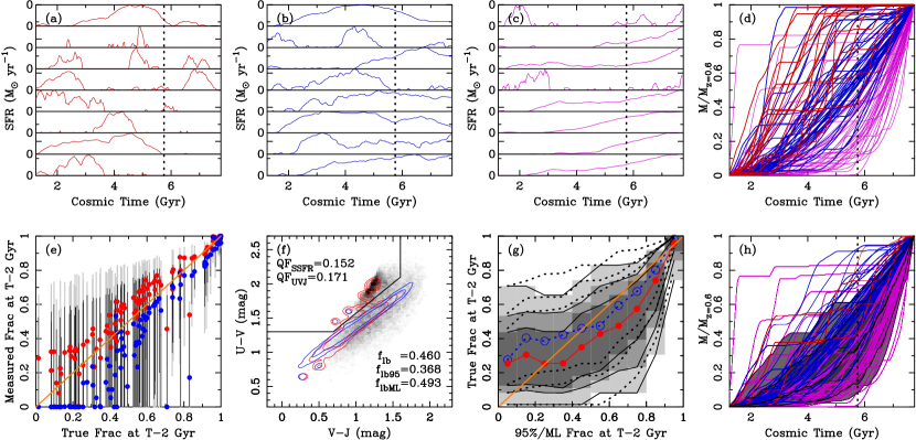
Figure A2.— Summary of the Model C simulations of mock galaxies at $z=0.6$ observed at $S/N=40$ per pixel. These simulations include simple screens of dust reddening in which the attenuation, $A_{V}$, is randomly selected uniformly up to an amount set by its ongoing SFR, with the entire population of $A_{V}$ normalized to a maximum $A_{V}=2$ mag. (a-c) Mock SFHs generated using the formalism of Kelson (2014) for use in simulating CSI’s ability to accurately measure the amounts of old stellar mass in systems. Red trajectories have low star formation activity at the epoch of observation, blue intermediate, and violet high. (d) Integrated growth trajectories for the 100 mock galaxies used in the simulations. (e) Distributions of measured best-fit (maximum likelihood, ML) ${\it z5fract2}$ for the 100 observations of each of 100 mock galaxies observed. Dark gray vertical bars extend over the 16th-84th percentiles of the ML measurements for each galaxy. The light gray extend over the 5th-95th percentiles. Blue circles show the median ML measurement for each mock galaxy, skewing to lower and lower values as the amount of old mass present decreases. Red circles show the median of the 95% upper limits derived from each mock measurement. Noise in the data skews the distribution of ML measurements such that the typical values are biased low. (f) Distribution of restframe $UVJ$ diagram for the mock galaxies. The quiescent galaxy fractions are shown, measured using $UVJ$ classification or classification by SSFR as measured by the last 200 Myr age bin. The quiescent fraction of this batch of simulated galaxies is $\sim 16\%$, low compared to the $\sim 40\%$ quiescent fraction in CSI for galaxies at $\log M>10$. Here the simulation also has a high intrinsic late bloomer fraction of 46%, underestimated by our ${\it z5fract2}_{95\%}$ selection criterion. Blue contours trace galaxies selected thusly to be late bloomers. Red contours show the distribution of the remaining galaxies. The grayscale in the background is the distribution of galaxies at $z\sim 0.6$ in CSI with stellar masses $\log M>10$. The mock galaxies reproduce the general morphology of the “quiescent clump” and star forming sequence, suggesting that simulations such as these, agnostic to assumptions about the forms of early SFHs, can provide a useful proxy for getting at systematic issues in SED fitting and estimates of early mass fractions. (g) Distribution of true ${\it z5fract2}$ values given different ${\it z5fract2}_{95\%}$ or ${\it z5fract2}_{ML}$ thresholds when selecting late growing mock galaxies. Blue circles trace the median true value of selected galaxies when using the ML ${\it z5fract2}$ measurements. Black dashed lines trace the 5th, 16th, 25th, 75th, 84th, and 95th percentiles. Red circles and solid black lines trace the equivalent percentiles when selecting late bloomers using ${\it z5fract2}_{95\%}$ instead of the maximum likelihood values. Selecting late bloomers using ${\it z5fract2}_{95\%}$ results in a purer identification of galaxies that grew the bulk of their stellar mass late. (h) Growth trajectories for the mock galaxies with observations that led to their selection as late bloomers. Shaded regions show the 5th, 16th, 84th, and 95th percentiles of these growth trajectories, to highlight the range of mass fractions captured by our LB selection criteria. An additional solid black line traces the 50th percentile.

Figure A2 quantitatively shows for Model C the measurements of mass in stars formed before $z=1$ relative to the mass measured at the epoch of observation ($z=0.6$). While these plots present a simple analysis of $10^{4}$ mock observations at $S/N=40$ per pixel, the basic picture only degrades significantly once one reaches $S/N\approx 10$. Overall these mock observations show that we can place strong constraints on the fraction of old stellar mass for individual galaxies.

Panels (a–c)

show example SFHs for mock galaxies in the simulations. Red, blue, and violet code trajectories for $\log{\dot{M}_{\ast}}/M_{\ast}<-10.5$, $-10.5\leq\log{\dot{M}_{\ast}}/M_{\ast}\leq-10$, and $\log{\dot{M}_{\ast}}/M_{\ast}>-10$, respectively, where $M_{\ast}=\int{\dot{M}_{\ast}}\,dt$. Note: these sSFRs reflect SFR on a $\sim$30 Myr timescale because the stochastic SFHs have 200 timesteps.

Panel (d)

shows the 100 growth trajectories using the same color coding. The Kelson (2014) non-Markovian stochastic SFHs naturally produce starforming and quiescent galaxies at a ratio of $\sim$5:1 (in their final 30 Myr timestep), which also holds in the late bloomer population. Hence, while most late bloomers are star-forming at T_obs, quite a few are not. Having simulations with both star-forming and quiescent LBs among the broad diversity of possible SFHs is critical for revealing what kind(s) of LBs we can reliably identify in CSI, or conversely whether CSI can help determine the duty cycles and frequencies with which galaxies may exit and/or enter the quiescent zone of, for example, the UVJ diagram.

Panel (e)

shows the distribution of best-fit, ${\it z5fract2}_{ML}$ estimates for each galaxy. Since each mock galaxy was observed 100 times, we have a well defined distribution of constraints on the mass present by $z=1$ for each one. Each vertical light (dark) gray bar extends over the 5^th–95^th (16^th–84^th) percentiles of the z5fract2_ML distributions for each mock galaxy. Blue filled circles show the medians. Below ${\it z5fract2}_{\rm true}\lower 1.29167pt\hbox{$\scriptscriptstyle\;\buildrel<\over{\sim}\;$}0.5$ it becomes increasingly difficult to detect and measure the presence of old stars using our techniques unless one has $S/N\lower 1.29167pt\hbox{$\scriptscriptstyle\;\buildrel>\over{\sim}\;$}100$ per pixel. At the typical CSI $S/N$, galaxies with low intrinsic fractions of stellar mass older than 2 Gyr are increasingly driven towards best-fit measurements containing identically zero old stars, and with increasing frequency.

That said, red circles in Figure A2e mark the medians of the 95% upper confidence limits on z5fract2 for each galaxy. When the best-fit solutions are consistent with zero old stars, our methodology maintains broad confidence limits, accurately reflecting the increased uncertainty on the old stellar mass so as to capture at least the potential for old stars to be present.

We again conclude that the right approach in CSI is to use the 95% ${\it z5fract2}$ upper-limits to identify LBs. These problems are likely to be generally applicable, hence classification by best-fit SFH properties should be performed with great caution.

Panel (f)

shows the distribution of “observed” UVJ colors for these mock galaxies in comparison to the UVJ colors of CSI galaxies at $z\sim 0.6$ and $\log M_{\ast}>10$. Blue contours to trace the mock LBs as classified by $z5fract2_{95\%}<0.5$; red contours trace the rest. The quiescent clump is consistent with CSI’s because those galaxies have very low intrinsic $A_{V}$, matching the dust-free mock galaxies. However, the star-forming mock galaxies in Figure A2 do not span the full range of CSI colors because this does require dust reddening (see Patel et al 2010).

Panel (g)

schematically traces the distributions of true ${\it z5fract2}$ given different ${\it z5fract2}_{95\%}$ and ${\it z5fract2}_{ML}$ observational selection thresholds. Perfect inferences of SFHs, and thus perfect ability to identify late bloomers, would trace the orange, diagonal, unity line. Observational noise results in errors and uncertainties in the inferred SFHs, quantified here as an increasing dispersion and (upward) bias in true ${\it z5fract2}$ values as the amount of old mass inferred from the SED fits decreases.

Blue circles trace the median true value of selected galaxies using ${\it z5fract2}_{ML}$. Black dashed lines trace the 5^th, 16^th, 25^th, 75^th, 84^th, and 95^th percentiles. Selecting late growing galaxies by ${\it z5fract2}_{ML}<0.5$ produces a sample where $\sim$75% intrinsically have ${\it z5fract2}\lower 1.29167pt\hbox{$\scriptscriptstyle\;\buildrel<\over{\sim}\;$}0.6$, and another 20% of reach up to ${\it z5fract2}\sim 0.85$.

The red circles and solid black lines trace the equivalent percentiles using ${\it z5fract2}_{95\%}$, instead. Here $\sim$84% of galaxies with measured ${\it z5fract2}_{95\%}<0.5$ intrinsically have ${\it z5fract2}\lower 1.29167pt\hbox{$\scriptscriptstyle\;\buildrel<\over{\sim}\;$}0.6$, and another $\sim$10% reach ${\it z5fract2}\sim 0.75$. Thus, selection of late bloomers by ${\it z5fract2}_{95\%}$ results in a purer sample.

Panel (h)

uses selection by ${\it z5fract2}_{95\%}$ to identify galaxies as (probable) LBs and shows their growth trajectories. The black lines trace the 5th, 16th, 50th, 84th, and 95th percentiles, to better illustrate the small fraction of the sample that are not true LBs. Identifying nontrivial samples of galaxies at $z\ll 1$ that have had such growth histories is a major challenge to notions that most normal and massive galaxies formed their stars and quenched early, leaving open the question of how such galaxies lingered for so long before experiencing rapid late-time growth. Furthermore, such galaxies break analytical approaches to ensemble galaxy evolution that do not explicitly account for the leap-frogging of subpopulations past others in their mass growth.

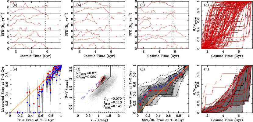
Figure A3.— Summary of the Model D simulations. Panels as in Figure A2.

A.2.4 Simulation Examples: Model D

Figure A3 shows the same information but for Model D—mock galaxies with ${\rm SFR}(\hbox{\emph{T${}_{\rm obs}$}})=0$. Overall these mock observations show that we can place strong constraints on the fraction of stellar mass already in place by $z=1$ for individual passive galaxies.

Even for mock galaxies where we have “observed” ${\it z5fract2}_{95\%}\sim 0.5$, 84% of such objects intrinsically have ${\it z5fract2}<0.6$.

Identifying nontrivial samples of quiescent galaxies at $z\ll 1$ that have had such growth histories allows us to better probe the dynamism hidden in the histories of galaxies that are largely viewed as “red and dead.” Measuring the late bloomer fractions in seemingly quiescent populations also quantifies the extent to which galaxies enter the red sequence and stop growing new stars for the remainders of their lifetimes.

A.2.5 Simulation Examples: The Effects of Subsolar Metallicities and Lower Signal-To-Noise Ratios

When $S/N$ ratios are insufficient to simultaneously constrain both the ages and metallicities of stellar population, SED fitting procedure(s) can produce results skewed by any input priors on stellar population metallicity—which in CSI are biased towards solar. To test the sensitivity of CSI’s ability to select late bloomers over a range of metallicities, we ran three variants of Model (C)— with stellar populations having solar metallicity, half-solar metallicity, and quarter-solar metallicity. Figure A4 recreates the final four panels of Figure A2 for these simulations at the three metallicities, and at $S/N=40$. The UVJ diagrams (b,f, and j) are, however, presented with violet contours that trace (75% of) the late bloomers in CSI. For comparison, the blue contours trace the distribution of mock galaxies that were selected by our fitting procedures to be late bloomers. Table 4 summarizes the key statistics from these simulations and for additional $S/N$ ratios than are displayed in these figures.

The key takeway from the simulations that vary metallicity and signal-to-noise ratio is that estimates of late bloomer fractions are only mildly sensitive to the range of signal-to-noise ratios being considered in the samples used in this paper. In contrast, our methodology for estimating a population’s late bloomer fraction is sensitive to the metallicity(ies) of the underlying stellar populations. Quantitatively, if the stellar populations in all galaxies selected by CSI as late bloomers had quarter-solar metallicity, then our analysis of their spectra makes $33\%-50\%$ more of them appear as late bloomers than are currently present. However, given past work on the ages and metallicities of galaxies at these epochs (see, e.g., Gallazzi et al. 2014) or the distributions of UVJ colors that are observed (see Panels b,f, and j). there is no evidence to suggest $[\hbox{Fe}/\hbox{H}]\approx-0.6$ dex is representative of the metallicities for a majority of the late bloomers identified by CSI. These simulations indicate that the effect is $\sim 20\%$ when the underlying galaxies identified as late bloomers have stellar populations with metallicities that are half-solar, i.e. bringing any observed estimate of $25\%$ down to $20\%$—a systematic error within our already stated levels of uncertainty.

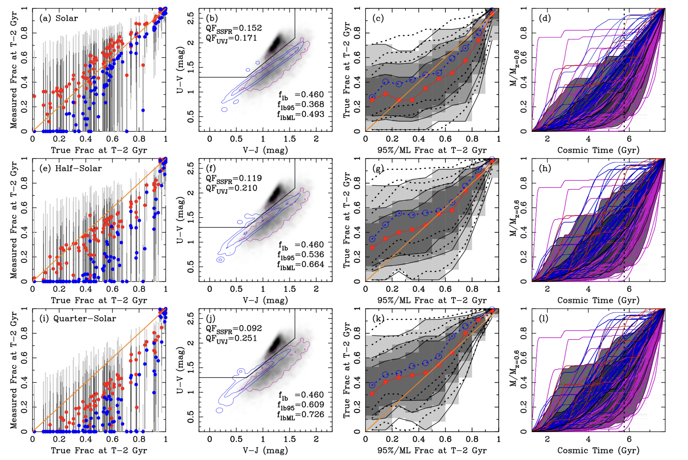
Figure A4.— Summary of the effects of metallicity using Model C at $S/N=40$. Each row is analogous to panels (e-h) of Figure A2, with the exception of the UVJ diagrams which now only show (blue) the distribution of mock galaxies selected to be late-bloomers after SED fitting, and (violet) the contour containing 75% of the late-bloomers in CSI with stellar masses above $10^{10}$ M_⊙. Top row shows the results for solar metallicity stellar populations. Center row shows the results of our template fitting when the galaxies have half-solar metallicity stellar populations. Bottom row shows the results of our template fitting when the galaxies have quarter-solar metallicity stellar populations.

Table 1Properties of CSI Galaxies in CANDELS/UDS

Panel	RA	DEC	$i$	$S/N$	$z$	$\log M_{\hbox{*}}\tablenotemark{a,b}$	Fractional Growth History				$n_{2}$
#			(mag)			$(M_{\odot})$	(2 Gyr)	(1 Gyr)	(0.5 Gyr)	(0.2 Gyr)	(Mpc-3)
1	2:17:48.94	-5:13:12.4	$21.94$	$17$	$0.652_{-0.007}^{+0.018}$	$10.00_{-0.02}^{+0.04}$	$0.00_{-0.00}^{+0.00}$	$0.73_{-0.02}^{+0.04}$	$0.84_{-0.09}^{+0.01}$	$0.95_{-0.03}^{+0.01}$	5.04
2	2:17:57.09	-5:11:00.5	$20.56$	$54$	$0.526_{-0.021}^{+0.021}$	$10.37_{-0.01}^{+0.04}$	$0.00_{-0.00}^{+0.00}$	$0.74_{-0.54}^{+0.16}$	$0.87_{-0.02}^{+0.03}$	$0.87_{-0.02}^{+0.03}$	1.53
3	2:17:43.38	-5:12:33.0	$20.97$	$35$	$0.656_{-0.007}^{+0.012}$	$10.34_{-0.02}^{+0.01}$	$0.00_{-0.00}^{+0.00}$	$0.49_{-0.01}^{+0.02}$	$0.89_{-0.07}^{+0.02}$	$0.93_{-0.02}^{+0.00}$	6.02
4	2:16:55.44	-5:09:01.5	$21.06$	$32$	$0.604_{-0.006}^{+0.037}$	$10.58_{-0.02}^{+0.12}$	$0.00_{-0.00}^{+0.00}$	$0.00_{-0.00}^{+0.72}$	$0.98_{-0.29}^{+0.02}$	$1.00_{-0.00}^{+0.00}$	1.99
5	2:17:37.05	-5:12:26.7	$21.94$	$18$	$0.656_{-0.011}^{+0.024}$	$10.02_{-0.02}^{+0.03}$	$0.00_{-0.00}^{+0.13}$	$0.00_{-0.00}^{+0.25}$	$0.98_{-0.27}^{+0.01}$	$0.99_{-0.00}^{+0.01}$	6.17
6	2:16:58.33	-5:07:52.4	$21.24$	$40$	$0.632_{-0.021}^{+0.008}$	$10.57_{-0.02}^{+0.03}$	$0.00_{-0.00}^{+0.00}$	$0.21_{-0.08}^{+0.38}$	$0.97_{-0.07}^{+0.00}$	$0.97_{-0.01}^{+0.01}$	2.92
7	2:17:11.68	-5:07:42.7	$22.18$	$15$	$0.714_{-0.030}^{+0.001}$	$10.24_{-0.05}^{+0.02}$	$0.00_{-0.00}^{+0.00}$	$0.76_{-0.39}^{+0.02}$	$0.98_{-0.00}^{+0.00}$	$0.98_{-0.00}^{+0.00}$	1.47
8	2:17:54.10	-5:12:49.9	$19.96$	$31$	$0.572_{-0.011}^{+0.007}$	$10.69_{-0.03}^{+0.01}$	$0.00_{-0.00}^{+0.00}$	$0.00_{-0.00}^{+0.31}$	$0.99_{-0.23}^{+0.01}$	$1.00_{-0.00}^{+0.00}$	1.16
9	2:17:37.81	-5:14:23.3	$21.62$	$15$	$0.684_{-0.013}^{+0.018}$	$10.38_{-0.02}^{+0.02}$	$0.00_{-0.00}^{+0.28}$	$0.00_{-0.00}^{+0.52}$	$0.98_{-0.41}^{+0.01}$	$0.98_{-0.00}^{+0.01}$	2.64
10	2:16:59.33	-5:16:23.7	$21.20$	$30$	$0.668_{-0.018}^{+0.015}$	$10.13_{-0.02}^{+0.01}$	$0.00_{-0.00}^{+0.00}$	$0.00_{-0.00}^{+0.34}$	$0.75_{-0.25}^{+0.04}$	$0.75_{-0.04}^{+0.04}$	2.91
11	2:17:27.41	-5:15:20.8	$20.34$	$36$	$0.458_{-0.007}^{+0.006}$	$10.25_{-0.02}^{+0.01}$	$0.00_{-0.00}^{+0.01}$	$0.93_{-0.06}^{+0.05}$	$0.98_{-0.01}^{+0.00}$	$0.98_{-0.01}^{+0.00}$	1.52
12	2:17:00.65	-5:10:31.6	$21.25$	$37$	$0.634_{-0.013}^{+0.009}$	$10.01_{-0.04}^{+0.03}$	$0.00_{-0.00}^{+0.00}$	$0.31_{-0.09}^{+0.08}$	$0.79_{-0.07}^{+0.09}$	$0.93_{-0.01}^{+0.00}$	3.16
13	2:17:29.56	-5:15:33.3	$21.58$	$25$	$0.658_{-0.010}^{+0.019}$	$10.44_{-0.03}^{+0.01}$	$0.00_{-0.00}^{+0.21}$	$0.05_{-0.01}^{+0.32}$	$0.93_{-0.55}^{+0.04}$	$0.96_{-0.00}^{+0.00}$	2.31
14	2:17:47.17	-5:08:46.3	$21.46$	$19$	$0.600_{-0.012}^{+0.006}$	$10.19_{-0.02}^{+0.01}$	$0.00_{-0.00}^{+0.00}$	$0.06_{-0.06}^{+0.32}$	$0.76_{-0.35}^{+0.14}$	$0.99_{-0.00}^{+0.01}$	1.33
15	2:16:53.85	-5:16:15.6	$20.98$	$57$	$0.754_{-0.008}^{+0.015}$	$10.05_{-0.01}^{+0.08}$	$0.00_{-0.00}^{+0.00}$	$0.00_{-0.00}^{+0.23}$	$0.00_{-0.00}^{+0.26}$	$0.40_{-0.05}^{+0.15}$	1.36
16	2:16:56.46	-5:12:57.4	$20.76$	$126$	$0.506_{-0.009}^{+0.004}$	$10.43_{-0.02}^{+0.01}$	$0.00_{-0.00}^{+0.00}$	$0.00_{-0.00}^{+0.13}$	$1.00_{-0.00}^{+0.00}$	$1.00_{-0.00}^{+0.00}$	0.32
17	2:17:18.69	-5:14:00.9	$21.46$	$20$	$0.590_{-0.010}^{+0.064}$	$10.17_{-0.02}^{+0.10}$	$0.00_{-0.00}^{+0.49}$	$0.08_{-0.02}^{+0.74}$	$0.93_{-0.20}^{+0.01}$	$0.93_{-0.01}^{+0.03}$	2.45
18	2:17:05.49	-5:12:44.7	$21.60$	$39$	$0.608_{-0.007}^{+0.017}$	$10.25_{-0.01}^{+0.03}$	$0.00_{-0.00}^{+0.00}$	$0.70_{-0.01}^{+0.04}$	$0.95_{-0.06}^{+0.00}$	$0.96_{-0.02}^{+0.00}$	2.09
19	2:17:22.99	-5:13:23.4	$21.94$	$19$	$0.656_{-0.036}^{+0.021}$	$10.21_{-0.03}^{+0.03}$	$0.00_{-0.00}^{+0.22}$	$0.74_{-0.02}^{+0.07}$	$0.87_{-0.13}^{+0.07}$	$0.92_{-0.01}^{+0.03}$	3.36
28				$21$	$0.642_{-0.013}^{+0.020}$	$10.25_{-0.06}^{+0.04}$	$0.43_{-0.43}^{+0.13}$	$0.43_{-0.43}^{+0.13}$	$0.97_{-0.07}^{+0.00}$	$0.97_{-0.02}^{+0.01}$	3.63
20	2:17:11.41	-5:15:56.4	$20.90$	$57$	$0.676_{-0.017}^{+0.008}$	$10.47_{-0.04}^{+0.03}$	$0.00_{-0.00}^{+0.00}$	$0.24_{-0.24}^{+0.35}$	$0.79_{-0.09}^{+0.13}$	$0.96_{-0.00}^{+0.00}$	2.65
21	2:17:42.14	-5:13:56.1	$22.55$	$17$	$0.676_{-0.032}^{+0.010}$	$10.22_{-0.04}^{+0.03}$	$0.06_{-0.06}^{+0.18}$	$0.98_{-0.04}^{+0.02}$	$1.00_{-0.00}^{+0.00}$	$1.00_{-0.00}^{+0.00}$	4.97
22	2:16:57.42	-5:14:45.3	$21.89$	$20$	$0.670_{-0.020}^{+0.022}$	$10.19_{-0.05}^{+0.03}$	$0.21_{-0.21}^{+0.26}$	$0.78_{-0.09}^{+0.08}$	$0.90_{-0.18}^{+0.06}$	$0.95_{-0.09}^{+0.01}$	2.41
23	2:16:58.70	-5:10:28.2	$21.38$	$46$	$0.642_{-0.008}^{+0.004}$	$10.32_{-0.03}^{+0.04}$	$0.32_{-0.24}^{+0.16}$	$0.32_{-0.08}^{+0.17}$	$1.00_{-0.09}^{+0.00}$	$1.00_{-0.00}^{+0.00}$	2.66
24	2:17:04.27	-5:13:25.9	$22.20$	$20$	$0.704_{-0.014}^{+0.009}$	$10.31_{-0.02}^{+0.03}$	$0.34_{-0.34}^{+0.18}$	$0.34_{-0.15}^{+0.21}$	$0.81_{-0.21}^{+0.17}$	$0.99_{-0.01}^{+0.00}$	1.62
69				$35$	$0.682_{-0.008}^{+0.007}$	$10.47_{-0.12}^{+0.03}$	$0.90_{-0.05}^{+0.01}$	$0.90_{-0.04}^{+0.02}$	$1.00_{-0.04}^{+0.00}$	$1.00_{-0.00}^{+0.00}$	2.09
25	2:16:59.73	-5:10:35.1	$22.31$	$21$	$0.654_{-0.016}^{+0.015}$	$10.26_{-0.06}^{+0.06}$	$0.36_{-0.36}^{+0.27}$	$0.61_{-0.06}^{+0.16}$	$1.00_{-0.00}^{+0.00}$	$1.00_{-0.00}^{+0.00}$	2.80
26	2:16:59.16	-5:12:56.7	$20.42$	$40$	$0.578_{-0.011}^{+0.005}$	$10.44_{-0.06}^{+0.07}$	$0.36_{-0.36}^{+0.33}$	$0.36_{-0.36}^{+0.33}$	$0.99_{-0.09}^{+0.01}$	$0.99_{-0.01}^{+0.01}$	1.00
27	2:17:12.00	-5:09:12.9	$21.91$	$23$	$0.640_{-0.012}^{+0.008}$	$10.20_{-0.03}^{+0.05}$	$0.38_{-0.06}^{+0.27}$	$0.66_{-0.04}^{+0.08}$	$1.00_{-0.00}^{+0.00}$	$1.00_{-0.00}^{+0.00}$	2.75
29	2:17:38.68	-5:15:53.0	$20.77$	$23$	$0.604_{-0.017}^{+0.010}$	$10.85_{-0.04}^{+0.05}$	$0.50_{-0.21}^{+0.21}$	$0.50_{-0.21}^{+0.21}$	$0.88_{-0.13}^{+0.12}$	$1.00_{-0.00}^{+0.00}$	3.38
30	2:17:44.51	-5:09:10.1	$21.39$	$16$	$0.762_{-0.008}^{+0.032}$	$10.81_{-0.05}^{+0.03}$	$0.50_{-0.50}^{+0.22}$	$0.50_{-0.24}^{+0.22}$	$0.88_{-0.20}^{+0.12}$	$1.00_{-0.00}^{+0.00}$	0.67
31	2:17:43.30	-5:14:04.4	$20.59$	$25$	$0.640_{-0.029}^{+0.014}$	$10.42_{-0.08}^{+0.05}$	$0.50_{-0.50}^{+0.08}$	$0.50_{-0.10}^{+0.08}$	$0.96_{-0.07}^{+0.01}$	$0.96_{-0.01}^{+0.01}$	5.45
32	2:17:33.01	-5:13:14.0	$22.01$	$34$	$0.634_{-0.009}^{+0.007}$	$10.32_{-0.01}^{+0.05}$	$0.51_{-0.13}^{+0.14}$	$0.72_{-0.17}^{+0.08}$	$1.00_{-0.00}^{+0.00}$	$1.00_{-0.00}^{+0.00}$	6.50
33	2:16:58.27	-5:11:02.7	$21.84$	$28$	$0.658_{-0.009}^{+0.009}$	$10.45_{-0.07}^{+0.05}$	$0.53_{-0.24}^{+0.23}$	$0.53_{-0.23}^{+0.23}$	$1.00_{-0.19}^{+0.00}$	$1.00_{-0.00}^{+0.00}$	2.98
34	2:17:34.33	-5:12:44.4	$21.91$	$26$	$0.640_{-0.008}^{+0.011}$	$10.28_{-0.06}^{+0.01}$	$0.57_{-0.23}^{+0.02}$	$0.57_{-0.23}^{+0.02}$	$1.00_{-0.05}^{+0.00}$	$1.00_{-0.00}^{+0.00}$	6.52
35	2:17:03.39	-5:09:40.9	$20.22$	$56$	$0.504_{-0.007}^{+0.003}$	$10.72_{-0.05}^{+0.04}$	$0.60_{-0.07}^{+0.16}$	$0.80_{-0.05}^{+0.05}$	$1.00_{-0.00}^{+0.00}$	$1.00_{-0.00}^{+0.00}$	0.52
36	2:17:33.54	-5:15:33.9	$21.70$	$39$	$0.590_{-0.008}^{+0.010}$	$10.03_{-0.04}^{+0.09}$	$0.61_{-0.41}^{+0.11}$	$0.61_{-0.06}^{+0.11}$	$1.00_{-0.00}^{+0.00}$	$1.00_{-0.00}^{+0.00}$	3.00
37	2:17:25.70	-5:12:43.7	$21.10$	$18$	$0.674_{-0.023}^{+0.016}$	$10.63_{-0.10}^{+0.01}$	$0.62_{-0.41}^{+0.02}$	$0.69_{-0.21}^{+0.24}$	$0.99_{-0.00}^{+0.00}$	$0.99_{-0.00}^{+0.00}$	2.30
38	2:16:55.47	-5:11:10.3	$22.20$	$18$	$0.664_{-0.020}^{+0.017}$	$10.27_{-0.10}^{+0.02}$	$0.62_{-0.62}^{+0.14}$	$0.74_{-0.17}^{+0.04}$	$1.00_{-0.25}^{+0.00}$	$1.00_{-0.00}^{+0.00}$	3.38
39	2:17:29.41	-5:12:25.4	$22.29$	$29$	$0.650_{-0.014}^{+0.012}$	$10.19_{-0.06}^{+0.02}$	$0.63_{-0.23}^{+0.01}$	$0.63_{-0.22}^{+0.01}$	$1.00_{-0.00}^{+0.00}$	$1.00_{-0.00}^{+0.00}$	4.62
40	2:17:53.28	-5:09:27.8	$21.15$	$19$	$0.644_{-0.005}^{+0.016}$	$10.24_{-0.02}^{+0.07}$	$0.63_{-0.02}^{+0.12}$	$0.63_{-0.02}^{+0.12}$	$0.81_{-0.11}^{+0.06}$	$0.94_{-0.03}^{+0.01}$	2.05
41	2:17:31.26	-5:12:17.2	$21.10$	$52$	$0.600_{-0.007}^{+0.008}$	$10.56_{-0.07}^{+0.01}$	$0.65_{-0.18}^{+0.06}$	$0.65_{-0.18}^{+0.06}$	$1.00_{-0.00}^{+0.00}$	$1.00_{-0.00}^{+0.00}$	3.07
42	2:16:55.69	-5:12:48.2	$20.99$	$48$	$0.638_{-0.010}^{+0.007}$	$10.63_{-0.06}^{+0.02}$	$0.65_{-0.19}^{+0.03}$	$0.65_{-0.19}^{+0.03}$	$1.00_{-0.08}^{+0.00}$	$1.00_{-0.00}^{+0.00}$	3.01
43	2:17:24.12	-5:15:56.1	$20.48$	$68$	$0.440_{-0.006}^{+0.004}$	$10.28_{-0.01}^{+0.08}$	$0.65_{-0.08}^{+0.14}$	$0.92_{-0.03}^{+0.02}$	$0.93_{-0.01}^{+0.01}$	$0.93_{-0.01}^{+0.01}$	1.73
44	2:17:55.57	-5:11:54.7	$22.14$	$16$	$0.632_{-0.014}^{+0.012}$	$10.36_{-0.06}^{+0.01}$	$0.67_{-0.23}^{+0.07}$	$0.67_{-0.22}^{+0.07}$	$0.81_{-0.10}^{+0.18}$	$1.00_{-0.00}^{+0.00}$	2.11
45	2:17:33.67	-5:12:04.1	$20.62$	$44$	$0.698_{-0.006}^{+0.006}$	$10.95_{-0.06}^{+0.01}$	$0.69_{-0.13}^{+0.03}$	$0.69_{-0.13}^{+0.03}$	$1.00_{-0.08}^{+0.00}$	$1.00_{-0.00}^{+0.00}$	2.44
46	2:17:05.65	-5:12:55.0	$21.39$	$40$	$0.632_{-0.015}^{+0.012}$	$10.57_{-0.01}^{+0.01}$	$0.71_{-0.08}^{+0.07}$	$0.71_{-0.08}^{+0.07}$	$0.88_{-0.09}^{+0.07}$	$1.00_{-0.00}^{+0.00}$	2.53
47	2:17:21.06	-5:08:56.7	$20.60$	$40$	$0.604_{-0.008}^{+0.009}$	$10.71_{-0.07}^{+0.01}$	$0.71_{-0.10}^{+0.04}$	$0.71_{-0.10}^{+0.04}$	$1.00_{-0.00}^{+0.00}$	$1.00_{-0.00}^{+0.00}$	1.24
48	2:17:27.08	-5:09:50.5	$21.21$	$41$	$0.610_{-0.007}^{+0.006}$	$10.59_{-0.06}^{+0.02}$	$0.72_{-0.08}^{+0.03}$	$0.72_{-0.08}^{+0.03}$	$1.00_{-0.07}^{+0.00}$	$1.00_{-0.00}^{+0.00}$	1.53
59				$43$	$0.588_{-0.006}^{+0.006}$	$10.53_{-0.01}^{+0.11}$	$0.82_{-0.06}^{+0.10}$	$0.87_{-0.01}^{+0.04}$	$1.00_{-0.00}^{+0.00}$	$1.00_{-0.00}^{+0.00}$	1.31
49	2:17:38.00	-5:13:09.9	$21.40$	$49$	$0.642_{-0.008}^{+0.008}$	$10.57_{-0.07}^{+0.02}$	$0.73_{-0.11}^{+0.05}$	$0.73_{-0.11}^{+0.05}$	$1.00_{-0.04}^{+0.00}$	$1.00_{-0.00}^{+0.00}$	6.78
50	2:17:33.78	-5:14:01.9	$20.61$	$38$	$0.662_{-0.010}^{+0.005}$	$10.97_{-0.06}^{+0.01}$	$0.73_{-0.12}^{+0.02}$	$0.73_{-0.12}^{+0.02}$	$0.90_{-0.10}^{+0.10}$	$1.00_{-0.00}^{+0.00}$	4.96
51	2:17:36.61	-5:13:34.2	$21.64$	$19$	$0.648_{-0.004}^{+0.010}$	$10.72_{-0.04}^{+0.06}$	$0.74_{-0.05}^{+0.18}$	$0.74_{-0.05}^{+0.18}$	$1.00_{-0.07}^{+0.00}$	$1.00_{-0.00}^{+0.00}$	6.10
52	2:17:25.59	-5:13:31.4	$20.39$	$45$	$0.630_{-0.008}^{+0.010}$	$10.96_{-0.10}^{+0.05}$	$0.75_{-0.15}^{+0.10}$	$0.75_{-0.15}^{+0.10}$	$0.99_{-0.05}^{+0.01}$	$1.00_{-0.00}^{+0.00}$	4.95
53	2:17:14.46	-5:15:46.0	$20.56$	$67$	$0.686_{-0.005}^{+0.003}$	$11.01_{-0.01}^{+0.03}$	$0.77_{-0.00}^{+0.05}$	$0.77_{-0.00}^{+0.05}$	$1.00_{-0.07}^{+0.00}$	$1.00_{-0.00}^{+0.00}$	1.71
54	2:17:08.28	-5:16:11.6	$21.46$	$36$	$0.682_{-0.013}^{+0.010}$	$10.65_{-0.07}^{+0.02}$	$0.78_{-0.11}^{+0.05}$	$0.78_{-0.09}^{+0.05}$	$1.00_{-0.01}^{+0.00}$	$1.00_{-0.00}^{+0.00}$	2.39
55	2:16:54.22	-5:14:56.4	$19.90$	$154$	$0.624_{-0.005}^{+0.002}$	$11.24_{-0.01}^{+0.01}$	$0.79_{-0.00}^{+0.01}$	$0.79_{-0.00}^{+0.01}$	$0.87_{-0.02}^{+0.01}$	$1.00_{-0.00}^{+0.00}$	2.24
56	2:17:09.69	-5:08:53.8	$21.44$	$38$	$0.634_{-0.014}^{+0.011}$	$10.54_{-0.07}^{+0.01}$	$0.79_{-0.08}^{+0.07}$	$0.89_{-0.05}^{+0.01}$	$1.00_{-0.00}^{+0.00}$	$1.00_{-0.00}^{+0.00}$	2.80
57	2:17:43.33	-5:13:30.6	$21.21$	$23$	$0.640_{-0.005}^{+0.010}$	$10.80_{-0.06}^{+0.03}$	$0.79_{-0.09}^{+0.10}$	$0.79_{-0.09}^{+0.10}$	$1.00_{-0.09}^{+0.00}$	$1.00_{-0.00}^{+0.00}$	5.31
62				$32$	$0.630_{-0.006}^{+0.012}$	$10.80_{-0.10}^{+0.04}$	$0.83_{-0.09}^{+0.08}$	$0.94_{-0.19}^{+0.00}$	$1.00_{-0.00}^{+0.00}$	$1.00_{-0.00}^{+0.00}$	5.41
58	2:17:28.93	-5:13:17.9	$21.28$	$30$	$0.604_{-0.010}^{+0.009}$	$10.69_{-0.05}^{+0.01}$	$0.81_{-0.09}^{+0.03}$	$0.81_{-0.09}^{+0.03}$	$1.00_{-0.05}^{+0.00}$	$1.00_{-0.00}^{+0.00}$	4.57
60	2:17:11.60	-5:09:01.0	$20.59$	$59$	$0.646_{-0.007}^{+0.002}$	$10.97_{-0.08}^{+0.01}$	$0.82_{-0.07}^{+0.00}$	$0.84_{-0.09}^{+0.00}$	$1.00_{-0.00}^{+0.00}$	$1.00_{-0.00}^{+0.00}$	2.86
67				$54$	$0.650_{-0.007}^{+0.003}$	$11.03_{-0.09}^{+0.01}$	$0.90_{-0.05}^{+0.00}$	$0.90_{-0.05}^{+0.00}$	$1.00_{-0.00}^{+0.00}$	$1.00_{-0.00}^{+0.00}$	3.03
61	2:17:38.95	-5:13:05.2	$21.11$	$31$	$0.652_{-0.007}^{+0.005}$	$10.78_{-0.07}^{+0.01}$	$0.83_{-0.08}^{+0.06}$	$0.83_{-0.08}^{+0.08}$	$1.00_{-0.11}^{+0.00}$	$1.00_{-0.00}^{+0.00}$	6.37
63	2:17:37.48	-5:14:31.1	$20.70$	$72$	$0.624_{-0.008}^{+0.006}$	$10.86_{-0.01}^{+0.08}$	$0.83_{-0.10}^{+0.04}$	$0.85_{-0.06}^{+0.09}$	$1.00_{-0.00}^{+0.00}$	$1.00_{-0.00}^{+0.00}$	5.27
64	2:17:31.04	-5:12:37.5	$21.57$	$50$	$0.636_{-0.006}^{+0.006}$	$10.58_{-0.07}^{+0.03}$	$0.84_{-0.07}^{+0.06}$	$0.84_{-0.07}^{+0.06}$	$1.00_{-0.08}^{+0.00}$	$1.00_{-0.00}^{+0.00}$	5.75
65	2:17:36.68	-5:13:41.2	$22.59$	$25$	$0.642_{-0.008}^{+0.007}$	$10.04_{-0.01}^{+0.11}$	$0.85_{-0.07}^{+0.05}$	$0.85_{-0.05}^{+0.06}$	$1.00_{-0.00}^{+0.00}$	$1.00_{-0.00}^{+0.00}$	6.39
66	2:17:31.86	-5:09:57.7	$20.14$	$64$	$0.498_{-0.006}^{+0.004}$	$10.94_{-0.09}^{+0.01}$	$0.87_{-0.06}^{+0.01}$	$0.87_{-0.06}^{+0.02}$	$1.00_{-0.00}^{+0.00}$	$1.00_{-0.00}^{+0.00}$	1.63
68	2:17:34.17	-5:13:39.3	$19.80$	$132$	$0.438_{-0.003}^{+0.002}$	$10.93_{-0.07}^{+0.01}$	$0.90_{-0.02}^{+0.07}$	$1.00_{-0.00}^{+0.00}$	$1.00_{-0.00}^{+0.00}$	$1.00_{-0.00}^{+0.00}$	0.84
70	2:17:38.16	-5:13:19.1	$20.80$	$56$	$0.634_{-0.006}^{+0.003}$	$10.93_{-0.08}^{+0.01}$	$0.92_{-0.06}^{+0.04}$	$0.97_{-0.02}^{+0.01}$	$1.00_{-0.01}^{+0.00}$	$1.00_{-0.00}^{+0.00}$	6.39
71	2:17:45.71	-5:13:27.7	$21.05$	$22$	$0.774_{-0.007}^{+0.007}$	$10.92_{-0.08}^{+0.02}$	$0.92_{-0.02}^{+0.01}$	$0.92_{-0.02}^{+0.01}$	$0.92_{-0.02}^{+0.01}$	$0.99_{-0.01}^{+0.00}$	1.10
72	2:17:14.97	-5:12:29.3	$21.87$	$30$	$0.760_{-0.008}^{+0.007}$	$10.45_{-0.09}^{+0.01}$	$0.93_{-0.04}^{+0.00}$	$0.93_{-0.03}^{+0.00}$	$0.93_{-0.03}^{+0.00}$	$0.98_{-0.01}^{+0.00}$	1.08
73	2:17:06.22	-5:13:17.8	$20.23$	$75$	$0.622_{-0.005}^{+0.003}$	$11.19_{-0.01}^{+0.01}$	$0.94_{-0.01}^{+0.00}$	$0.94_{-0.01}^{+0.00}$	$0.99_{-0.01}^{+0.01}$	$1.00_{-0.00}^{+0.00}$	2.32
74	2:17:29.02	-5:15:49.1	$21.57$	$27$	$0.772_{-0.012}^{+0.008}$	$10.67_{-0.07}^{+0.03}$	$0.96_{-0.01}^{+0.01}$	$0.96_{-0.01}^{+0.01}$	$0.96_{-0.01}^{+0.01}$	$0.96_{-0.01}^{+0.01}$	1.40
75	2:17:44.55	-5:15:22.3	$19.37$	$138$	$0.490_{-0.004}^{+0.001}$	$11.11_{-0.01}^{+0.02}$	$0.96_{-0.01}^{+0.04}$	$1.00_{-0.00}^{+0.00}$	$1.00_{-0.00}^{+0.00}$	$1.00_{-0.00}^{+0.00}$	1.32
79				$86$	$0.488_{-0.006}^{+0.004}$	$11.28_{-0.01}^{+0.01}$	$0.98_{-0.01}^{+0.00}$	$0.98_{-0.01}^{+0.00}$	$1.00_{-0.00}^{+0.00}$	$1.00_{-0.00}^{+0.00}$	1.31
76	2:17:36.32	-5:11:01.1	$21.40$	$32$	$0.492_{-0.007}^{+0.007}$	$10.48_{-0.01}^{+0.01}$	$0.96_{-0.02}^{+0.00}$	$0.96_{-0.02}^{+0.00}$	$1.00_{-0.00}^{+0.00}$	$1.00_{-0.00}^{+0.00}$	1.57
77	2:17:29.91	-5:08:44.1	$21.23$	$27$	$0.490_{-0.010}^{+0.011}$	$10.50_{-0.12}^{+0.01}$	$0.96_{-0.04}^{+0.03}$	$0.96_{-0.02}^{+0.03}$	$1.00_{-0.03}^{+0.00}$	$1.00_{-0.00}^{+0.00}$	1.33
78	2:18:01.19	-5:08:22.4	$21.07$	$53$	$0.564_{-0.007}^{+0.005}$	$10.75_{-0.01}^{+0.01}$	$0.97_{-0.01}^{+0.00}$	$0.97_{-0.01}^{+0.00}$	$1.00_{-0.02}^{+0.00}$	$1.00_{-0.00}^{+0.00}$	1.80
80	2:17:45.53	-5:10:06.9	$21.76$	$16$	$0.518_{-0.010}^{+0.010}$	$10.33_{-0.15}^{+0.03}$	$0.99_{-0.02}^{+0.01}$	$0.99_{-0.02}^{+0.01}$	$0.99_{-0.01}^{+0.00}$	$1.00_{-0.00}^{+0.00}$	1.42

Note. — Confidence intervals reflect formal/random errors only.

Table 2True and Recovered LBFs and Purity of Selection of Simulated Data

Model	QF	LBF	LBF${}_{ML}(P_{ML})$	LBF${}_{95\%}(P_{95\%})$
(A) $A_{V}=0$	0.15	0.46	$0.58(0.70)$	${\bf 0.43}(0.76)$
(B) $\hbox{max}A_{V}=1$	0.15	0.46	$0.49(0.69)$	${\bf 0.35}(0.76)$
(C) $\hbox{max}(A_{V})\propto\log{\dot{M}}_{z=0.6}$	0.15	0.46	$0.49(0.69)$	${\bf 0.37}(0.75)$
(D) ${\dot{M}}_{z=0.6}=0$, $A_{V}=0$	0.87	0.07	$0.15(0.44)$	${\bf 0.11}(0.55)$
(E) $3:1$ mix of B $+$ Dead	0.17	0.27	$0.41(0.46)$	${\bf 0.28}(0.51)$

Table 3Late Bloomer Fractions and Purity of Selection in Simulated Data by Star Forming Activity

	Star Forming				Quiescent
Model	LBF	LBFML	LBF95%		LBF	LBFML	LBF95%
(A)	0.53	$0.67(0.70)$	${\bf 0.50}(0.77)$		0.06	$0.07(0.42)$	${\bf 0.05}(0.44)$
(B)	0.53	$0.55(0.71)$	${\bf 0.40}(0.77)$		0.06	$0.11(0.31)$	${\bf 0.06}(0.40)$
(C)	0.53	$0.57(0.70)$	${\bf 0.43}(0.76)$		0.06	$0.07(0.41)$	${\bf 0.04}(0.39)$
(D)	0.32	$0.47(0.64)$	${\bf 0.39}(0.74)$		0.02	$0.09(0.24)$	${\bf 0.06}(0.31)$
(E)	0.32	$0.46(0.48)$	${\bf 0.32}(0.52)$		0.00	$0.11(0.00)$	${\bf 0.06}(0.00)$

Table 4The Effects of $S/N$ Ratio and Uncertain Metallicity on True and Recovered LBFs and Purity with Simulated Data using Model (C)

$S/N$ Ratio	$[\hbox{Fe}/\hbox{H}]$	LBF	LBF${}_{ML}(P_{ML})$	LBF${}_{95\%}(P_{95\%})$
40	0.0	0.46	$0.49(0.69)$	${\bf 0.37}(0.75)$
40	-0.3	0.46	$0.66(0.60)$	${\bf 0.54}(0.67)$
40	-0.6	0.46	$0.73(0.59)$	${\bf 0.61}(0.63)$
20	0.0	0.46	$0.50(0.65)$	${\bf 0.35}(0.69)$
20	-0.3	0.46	$0.69(0.56)$	${\bf 0.54}(0.61)$
20	-0.6	0.46	$0.79(0.52)$	${\bf 0.65}(0.55)$
10	0.0	0.46	$0.54(0.61)$	${\bf 0.34}(0.66)$
10	-0.3	0.46	$0.69(0.53)$	${\bf 0.51}(0.59)$
10	-0.6	0.46	$0.84(0.47)$	${\bf 0.67}(0.49)$

References

- Abramson et al. (2013) Abramson, L. E., Dressler, A., Gladders, M. D., et al. 2013, ApJ, 777, 124
- Abramson et al. (2015) Abramson, L. E., Gladders, M. D., Dressler, A., et al. 2015b, ApJ, 801, L12 (A15)
- Abramson et al. (2016) Abramson, L. E., Gladders, M. D., Dressler, A., et al. 2016, ApJ, 832, 7 (A16)
- Abramson et al. (2017) Abramson, L. E., Newman, A. B., Treu, T., et al. 2017, arXiv:1710.00843
- Behroozi et al. (2013) Behroozi, P. S., Marchesini, D., Wechsler, R. H., et al. 2013, ApJ, 777, L10
- Behroozi et al. (2013) Behroozi, P. S., Wechsler, R. H., & Conroy, C. 2013, ApJ, 770, 57
- Bell et al. (2006) Bell, E. F., Phleps, S., Somerville, R. S., et al. 2006, ApJ, 652, 270
- Benson (2012) Benson, A. J. 2012, NewAstron., 17, 175
- Calzetti et al. (2000) Calzetti, D., Armus, L., Bohlin, R. C., et al. 2000, ApJ, 533, 682
- Chauke et al. (2018) Chauke, P., van der Wel, A., Pacifici, C., et al. 2018, arXiv:1805.02568
- Conroy et al. (2009) Conroy, C., Gunn, J. E., & White, M. 2009, ApJ, 699, 486
- Conroy & Gunn (2010) Conroy, C., & Gunn, J. E. 2010, ApJ, 712, 833
- Cowie et al. (1996) Cowie, L. L., Songaila, A., Hu, E. M., & Cohen, J. G. 1996, AJ, 112, 839
- Dalcanton et al. (2012) Dalcanton, J. J., Williams, B. F., Lang, D., et al. 2012, ApJS, 200, 18
- Davis & Geller (1976) Davis, M., & Geller, M. J. 1976, ApJ, 208, 13
- Dickinson et al. (2003) Dickinson, M., Papovich, C., Ferguson, H. C., & Budavári, T. 2003, ApJ, 587, 25
- Dressler (1980) Dressler, A. 1980, ApJ, 236, 351
- Dressler et al. (2011) Dressler, A., Bigelow, B., Hare, T., et al. 2011, PASP, 123, 288
- Dressler et al. (2016) Dressler, A., Kelson, D. D., Abramson, L. E., et al. 2016, ApJ, 833, 251 (D16)
- Faber et al. (2007) Faber, S. M., Willmer, C. N. A., Wolf, C., et al. 2007, ApJ, 665, 265
- Gallagher et al. (1984) Gallagher, J. S., III, Hunter, D. A., & Tutukov, A. V. 1984, ApJ, 284, 544
- Gallazzi et al. (2014) Gallazzi, A., Bell, E. F., Zibetti, S., Brinchmann, J., & Kelson, D. D. 2014, ApJ, 788, 72
- Giocoli et al. (2012) Giocoli, C., Tormen, G., & Sheth, R. K. 2012, MNRAS, 422, 185
- Gladders et al. (2013) Gladders, M. D., Oemler, A., Dressler, A., et al. 2013, ApJ, 770, 64 (G13)
- Iyer & Gawiser (2017) Iyer, K., & Gawiser, E. 2017, ApJ, 838, 127
- Kelson et al. (2014) Kelson, D. D., Williams, R. J., Dressler, A., et al. 2014a, ApJ, 783, 110 (K14)
- Kelson (2014) Kelson, D. D. 2014b, arXiv:1406.5191
- Kelson et al. (2016) Kelson, D. D., Benson, A. J., & Abramson, L. E. 2016, arXiv:1610.06566
- Knebe et al. (2018) Knebe, A., Stoppacher, D., Prada, F., et al. 2018, MNRAS, 474, 5206
- Koekemoer et al. (2011) Koekemoer, A. M., Faber, S. M., Ferguson, H. C., et al. 2011, ApJS, 197, 36
- Lanzetta et al. (1995) Lanzetta, K. M., Wolfe, A. M., & Turnshek, D. A. 1995, ApJ, 440, 435
- Leitner (2012) Leitner, S. N. 2012, Ph.D. Thesis,
- Lilly et al. (1996) Lilly, S. J., Le Fevre, O., Hammer, F., & Crampton, D. 1996, ApJ, 460, L1
- Lonsdale et al. (2003) Lonsdale, C. J., Smith, H. E., Rowan-Robinson, M., et al. 2003, PASP, 115, 89
- Loveday et al. (1995) Loveday, J., Maddox, S. J., Efstathiou, G., & Peterson, B. A. 1995, ApJ, 442, 457
- Madau & Dickinson (2014) Madau, P., & Dickinson, M. 2014, ARA&A, 52, 415 (MD14)
- Man et al. (2016) Man, A. W. S., Zirm, A. W., & Toft, S. 2016, ApJ, 830, 89
- Martínez-García et al. (2017) Martínez-García, E. E., Bruzual, G., Magris, G., & González-Lópezlira, R. A. 2017, arXiv:1710.09402
- Noeske et al. (2007) Noeske, K. G., Weiner, B. J., Faber, S. M., et al. 2007, ApJ, 660, L43
- Oemler et al. (2013b) Oemler, A., Jr., Dressler, A., Gladders, M. G., et al. 2013a, ApJ, 770, 63 (O13)
- Oesch et al. (2017) Oesch, P. A., Bouwens, R. J., Illingworth, G. D., Labbe, I., & Stefanon, M. 2017, arXiv:1710.11131
- Pacifici et al. (2013) Pacifici, C., Kassin, S. A., Weiner, B., Charlot, S., & Gardner, J. P. 2013, ApJ, 762, L15
- Pacifici et al. (2016) Pacifici, C., Kassin, S. A., Weiner, B. J., et al. 2016, ApJ, 832, 79
- Pei & Fall (1995) Pei, Y. C., & Fall, S. M. 1995, ApJ, 454, 69
- Peng et al. (2010) Peng, Y.-j., Lilly, S. J., Kovač, K., et al. 2010, ApJ, 721, 193
- Rowlands et al. (2018) Rowlands, K., Wild, V., Bourne, N., et al. 2018, MNRAS, 473, 1168
- Schawinski et al. (2014) Schawinski, K., Urry, C. M., Simmons, B. D., et al. 2014, MNRAS, 440, 889
- Speagle et al. (2014) Speagle, J. S., Steinhardt, C. L., Capak, P. L., & Silverman, J. D. 2014, ApJS, 214, 15
- Tinsley (1972) Tinsley, B. M. 1972, A&A, 20, 383
- Tomczak et al. (2016) Tomczak, A. R., Quadri, R. F., Tran, K.-V. H., et al. 2016, ApJ, 817, 118
- Torrey et al. (2017) Torrey, P., Wellons, S., Ma, C.-P., Hopkins, P. F., & Vogelsberger, M. 2017, MNRAS, 467, 4872
- Treu et al. (2005) Treu, T., Ellis, R. S., Liao, T. X., et al. 2005, ApJ, 633, 174
- Vogelsberger et al. (2014) Vogelsberger, M., Genel, S., Springel, V., et al. 2014, MNRAS, 444, 1518
- Whitaker et al. (2012) Whitaker, K. E., van Dokkum, P. G., Brammer, G., & Franx, M. 2012, ApJ, 754, L29
- Williams et al. (2011) Williams, R. J., Quadri, R. F., & Franx, M. 2011, ApJ, 738, L25