Beyond $\mathcal{R}(D^{(*)})$ with the general 2HDM-III for $b\to c\tau\nu$

Abstract

We review the parameter regions allowed by measurements of $\mathcal{R}(D^{(*)})$ and by a theoretical limit on ${\cal B}(B_{c}\to\tau\nu)$ in terms of generic scalar and pseudoscalar new physics couplings, $g_{s}$ and $g_{p}$. We then use these regions as constraints to predict the ranges for additional observables in $b\to c\tau\nu$ including the differential decay distributions $d\Gamma/dq^{2}$; the ratios $\mathcal{R}(J/\psi)$ and $\mathcal{R}(\Lambda_{c})$; and the tau-lepton polarisation in $B\to D^{(\star)}\tau\nu$, with emphasis on the CP violating normal polarisation. Finally we map the allowed regions in $g_{s}$ and $g_{p}$ into the parameters of four versions of the Yukawa couplings of the general 2HDM-III model. We find that the model is still viable but could be ruled out by a confirmation of a large $\mathcal{R}(J/\psi)$.

1 Introduction

Amongst the most interesting current results in B physics, the searches for lepton universality in semileptonic B decays stand out. On the experimental side, hints at deviations from the standard model (SM) in some of these modes have existed for several years, with $\bar{B}\to D\tau\nu$ being measured by BaBar [1, 2] and Belle [3]; and with $\bar{B}\to D^{\star}\tau\nu$ being measured by BaBar [1, 2], Belle [3, 4, 5] and LHCb [6, 7]. On the theoretical side, many extensions of the SM violate lepton universality whereas the SM does not. The tests involve comparing semileptonic B decays into tau-leptons to those with muons and electrons through ratios such as,

$$\mathcal{R}(D^{(*)})=\frac{\Gamma(\bar{B}\to D^{(*)}\tau\bar{\nu})}{\Gamma(\bar{B}\to D^{(*)}l\bar{\nu})},$$ (1)

where $l$ represents either $e$ or $\mu$. The current values for these quantities hint to the existence of new physics, as can be seen when comparing the current HFLAV averages [8],

$$\mathcal{R}(D) = 0.407\pm 0.039\pm 0.024$$

$$\mathcal{R}(D^{\star}) = 0.304\pm 0.013\pm 0.007\ ,$$ (2)

to the current SM predictions from the lattice for $\mathcal{R}(D)$ [9, 10] or from a range of models for $\mathcal{R}(D^{\star})$ [11, 12],

$$\mathcal{R}_{SM}(D) = 0.299\pm 0.011$$

$$\mathcal{R}_{SM}(D^{\star}) = 0.252\pm 0.003\ .$$ (3)

For our new calculations in this paper, we will use the CCQM model for form factors which yields somewhat lower values for these quantities albeit with larger errors, $\mathcal{R}_{SM}(D)=0.27\pm 0.03$ and $\mathcal{R}_{SM}(D^{\star})=0.24\pm 0.02$.

A related measurement, $B_{c}^{+}\to J/\psi\tau^{+}{\nu}_{\tau}$, has been reported by LHCb [13] and also hints to disagreement with the SM, although the errors are too large at present to reach a definitive conclusion,

$$\mathcal{R}(J/\psi) = \frac{\Gamma(B_{c}^{+}\to J/\psi\tau^{+}{\nu}_{\tau})}{\Gamma(B_{c}^{+}\to J/\psi\mu^{+}{\nu}_{\mu})}$$ (4)

$$= 0.71\pm 0.17\pm 0.18\ .$$

Different predictions for the SM arising from different models for form factors produce a range $0.24$ to $0.28$ [14, 15, 16, 17, 18] which is about 2$\sigma$ lower that the LHCb result. With the CCQM form factors we obtain

$$\mathcal{R}(J/\psi)_{SM}=0.24\pm 0.02\ ,$$ (5)

which we use as the SM prediction in our numerical analysis.

Not surprisingly, these anomalies have generated enormous interest in the community. From the experimental side, we expect a measurement of the corresponding ratio for semileptonic $\Lambda_{b}\to\Lambda_{c}\tau\nu$, $\mathcal{R}(\Lambda_{c})$ to be reported soon. From the theory side there have been several proposals for additional observables to be studied in connection with these modes such as the tau-lepton polarisation [19, 20, 21, 22, 23, 24]. In fact, the Belle collaboration has already reported a result for the longitudinal tau polarisation in $\bar{B}\to D^{*}\tau^{-}\bar{\nu}_{\tau}$ [5]

$$P_{L}^{\tau}(D^{*})=-0.38\pm 0.51_{-0.16}^{+0.21},$$ (6)

a result in agreement with the SM prediction [19]

$$P_{L}^{\tau}(D^{*})_{SM}=-0.497\pm 0.013,$$ (7)

albeit with large uncertainty.

There have also been a large number of theory papers interpreting these results in the context of specific models, including additional Higgs doublets, gauge bosons and leptoquarks [25, 26, 27, 28, 29, 30, 31, 32, 33, 34, 35, 19, 36, 37, 38, 39, 40, 41, 42, 43, 44, 45, 46, 47, 48, 49, 50, 23, 51, 52, 53, 54, 55, 56]. One of the first possibilities considered was the 2HDM type II, where BaBar [2] determined it was not possible to simultaneously fit $\mathcal{R}(D)$ and $\mathcal{R}(D^{\star})$. However, a charged Higgs with couplings proportional to fermion masses is an obvious candidate to explain non-universality in semitauonic decays, prompting consideration of the more general 2HDM-III. Several authors have examined the flavour phenomenology of the 2HDM-III in the context of the anomalies mentioned above. Refs. [27, 19, 57] concluded that it is possible to explain $\mathcal{R}(D)$ and $\mathcal{R}(D^{\star})$ in this way after considering existing flavour physics constraints. More recently, Ref. [23, 58], add an analysis of the longitudinal tau-lepton polarisation and forward-backward asymmetries in $b\to c/u\ \tau\nu$ decays within the 2HDM-III.

In this paper we revisit the $b\to c\tau\nu$ modes in the presence of new (pseudo)-scalar operators to include several new results. We begin in Section II with a review of the constraints imposed by the measurements of $\mathcal{R}(D^{(*)})$ and the theoretical limit on ${\cal B}(B_{c}\to\tau\nu)$ [59, 60]. We then use these constraints to obtain the predicted ranges for $\mathcal{R}(J/\psi)$, the tau polarisation in $B\to D^{(*)}\tau\nu$ decays, the differential decay rates and the ratio $\mathcal{R}(\Lambda_{c})$ in Section III. We pay particular attention to the transverse tau polarisation which is $T$-odd [20, 21, 61, 62, 63, 64, 65] as the 2HDM-III model allows for CP violation and would naturally give rise to this effect. We also consider the $d\Gamma/dq^{2}$ distributions [40] in $B\to D^{(*)}\tau\nu$ but find that they offer no discriminating power in this case. They do serve to illustrate the CCQM model for the form factors. In Section IV we review the basics of the general two Higgs doublet model and the four different parameterizations for its Yukawa couplings. We then map this parameter space into the generic allowed regions obtained in Section II, finding they are completely accessible to this model. Finally, in Section V we conclude.

2 $b\to c\tau\nu$ constraints on new (pseudo)-scalar couplings

The effective Hamiltonian responsible for $b\to c\tau\nu$ transitions that results from the SM plus the 2HDM-III can be written in terms of the SM plus generic scalar operators in the form,

$$\begin{array}[]{l}{\cal H}_{{\rm eff}}=C_{SM}^{cb}{\cal O}_{SM}^{cb}+C_{R}^{cb}{\cal O}_{R}^{cb}+C_{L}^{cb}{\cal O}_{L}^{cb},\end{array}$$ (8)

where $C_{SM}^{cb}=4G_{F}V_{cb}/\sqrt{2}$ and the operators are given by

$$\begin{array}[]{l}{\cal O}_{SM}^{cb}=\left(\bar{c}\gamma_{\mu}P_{L}b\right)\left(\bar{\tau}\gamma_{\mu}P_{L}\nu_{\tau}\right),\\ {\cal O}_{R}^{cb}=\left(\bar{c}P_{R}b\right)\left(\bar{\tau}P_{L}\nu_{\tau}\right),\\ {\cal O}_{L}^{cb}=\left(\bar{c}P_{L}b\right)\left(\bar{\tau}P_{L}\nu_{\tau}\right).\end{array}$$ (9)

As the existing constraints will apply separately to the scalar and the pseudoscalar couplings, it is convenient to define

$$g_{S}\equiv\frac{C_{R}^{cb}+C_{L}^{cb}}{C_{SM}^{cb}},\ g_{P}\equiv\frac{C_{R}^{cb}-C_{L}^{cb}}{C_{SM}^{cb}}.$$ (10)

The effect of the effective Hamiltonian, Eq. 8, on the ratios $\mathcal{R}(D^{(*)})$ is known in the literature [11, 27, 57] and can be written as ratios $r_{D^{(*)}}={\cal R}(D^{(*)})/{\cal R}_{SM}(D^{(*)})$,

$$r_{D} = 1+1.5\ \textrm{Re}\left(g_{S}\right)+1.0\ \left|g_{S}\right|^{2},$$

$$r_{D^{*}} = 1+0.12\ \textrm{Re}\left(g_{P}\right)+0.05\ \left|g_{P}\right|^{2}.$$ (11)

A few remarks are in order. First, Refs. [30, 57] observe that the coefficient of $|g_{S}|^{2}$ can be changed from 1.0 to 1.5 to approximate some detector effects in BaBar. As we use the HFLAV average value for $r_{D}$ from both BaBar and Belle results, we will not include this correction in our numerics. Second, the CCQM model we use for the form factors leads to the slightly different expression $r_{D^{*}}=1+0.1\ \textrm{Re}(g_{P})+0.03\ |g_{P}|^{2}$, but with larger theoretical errors. We will discuss the effect of this below.

It is also known that there are values of $C_{L}^{cb}$ and $C_{R}^{cb}$ that can explain both of these ratios, and that the possible solutions become tightly constrained when one also requires that ${\mathcal{B}}(B_{c}\to\tau\nu)\leq 30\%$ [59], which for NP given by scalar operators implies that the ratio

$$\frac{{\cal B}(B_{c}\to\tau\nu)}{{\cal B}(B_{c}\to\tau\nu)_{SM}}=\left|1+\frac{m_{B_{c}}^{2}}{m_{\tau}(m_{b}+m_{c})}g_{P}\right|^{2}$$ (12)

be smaller than around 14.6. An even tighter constraint, by a factor of three, is advocated in Ref. [60].

We summarize these results in Figure 1. On the left panel we consider the constraint on $g_{S}$ which arises solely from satisfying ${\cal R}(D)$ at the $2\sigma$ level and appears as the blue ring. The black ring shows the effect of approximating the BaBar detector effects as suggested by Refs. [30, 57]. The central panel shows the constraints on $g_{P}$: the red ring arising from satisfying $r_{D^{*}}$ at the $2\sigma$ level and the green circle from ${\mathcal{B}}(B_{c}\to\tau\nu)\leq 30\%$. The small combined allowed region shows the tension between these two requirements. On the right panel we illustrate these combined constraints on $g_{P}$ as the red crescent shape. If one adopts the condition ${\mathcal{B}}(B_{c}\to\tau\nu)\leq 10\%$ [60] instead, there is no allowed region that also satisfies $r_{D^{*}}$ at the $2\sigma$ level, but there is one at the $3\sigma$ level and we show this in black. As mentioned above, the expression for $r_{D^{*}}$ with the CCQM form factors is slightly different but with larger errors which allow a larger overlap with ${\mathcal{B}}(B_{c}\to\tau\nu)\leq 30\%$ and this is shown as the orange crescent. For our predictions in the next section we will use the blue ring in the left panel and the red crescent in the right panel. Some, but not all, of these results have appeared before in the literature. For example Refs. [66, 67] do not include a constraint from ${\mathcal{B}}(B_{c}\to\tau\nu)$ in their results.

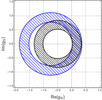
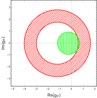
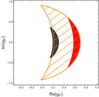
Figure 1: Left panel: the blue ring indicates the region allowed by ${\cal R}(D)$ at the $2\sigma$ level and the black ring shows how this region is modified following the prescription of Refs. [30, 57] described in the text. Center panel: the red ring indicates the region allowed by ${\cal R}(D^{*})$ at the $2\sigma$ level and the green circle results in ${\mathcal{B}}(B_{c}\to\tau\nu)\leq 30\%$. The small crescent region where these two intersect is the constraint of $g_{P}$ that we use for our predictions. This region is magnified as the red crescent on the right panel where it is also compared with the larger orange region which uses the CCQM form factors for ${\cal R}(D^{*})$, and with the black region which shows the intersection between ${\cal R}(D^{*})$ at the $3\sigma$ level and ${\mathcal{B}}(B_{c}\to\tau\nu)\leq 10\%$.

3 Predictions

3.1 Differential decay distributions for $B\to D^{(\star)}\tau\nu$.

In Figure 2 we compare the distributions $d\Gamma/dq^{2}$ for $B\to D^{(\star)}\tau\nu$ using the CCQM form factors with parameter values from Ref. [66]. The results indicate that the predicted spectrum is in good agreement with the measurements within the CCQM uncertainties (which the authors of Ref. [66] estimate at about 10%). The modifications to these predictions from $g_{P}$ and $g_{S}$ as constrained above are indistinguishable from the SM within this level of accuracy.

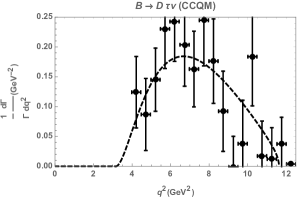
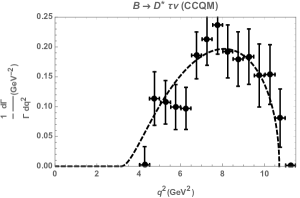
Figure 2: Normalised distributions $d\Gamma(B\to D\tau\nu)/(\Gamma dq^{2})$ (left) and $d\Gamma(B\to D^{\star}\tau\nu)/(\Gamma dq^{2})$ (right) as measured by BaBar [2] compared to the predictions in the SM with form factors from the CCQM of Ref. [66].

3.2 $\mathcal{R}(J/\psi)$

As already mentioned, there is also a more recent measurement of $\mathcal{R}(J/\psi)$ given in Eq. 4, which can be used as an additional test of the model. Using the form factors shown in the appendix with CCQM values from Ref. [68], this can be written in terms of generic scalar coefficients as

$$r_{J/\psi} \equiv \frac{\mathcal{R}(J/\psi)}{\mathcal{R}(J/\psi)_{SM}}\approx 1+0.09\ \textrm{Re}\left(g_{P}\right)+0.03\ \left|g_{P}\right|^{2}.$$ (13)

Note that this result is almost identical to that for $r_{D^{\star}}$ when the CCQM form factors are used for that case as well. The differential distribution $d\Gamma/dq^{2}$ for $B_{c}\to J/\psi\tau\nu$ receives tiny corrections from $g_{S,P}$ as constrained above, making it indistinguishable form the SM one. In Figure 3 we show the prediction for $\mathcal{R}(J/\psi)$ that is consistent with the measured $\mathcal{R}(D^{\star})$ at $2\sigma$ as well as ${\mathcal{B}}(B_{c}\to\tau\nu)\leq 30\%$. The largest prediction ($\sim 1.075$) is about $1.5\sigma$ away from the LHCb measurement thanks to its present large uncertainty, which in terms of this ratio is $r_{J/\psi}=2.5\pm 1.0$. A confirmation of a large value for $r_{J/\psi}$ can potentially rule out (pseudo)-scalar explanations of these anomalies.

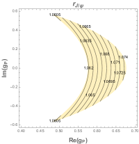
Figure 3: Predictions for $r_{J/\psi}$ compatible with the measured $\mathcal{R}(D^{\star})$ at $2\sigma$ as well as ${\mathcal{B}}(B_{c}\to\tau\nu)\leq 30\%$.

3.3 Polarisations

In general, we can define normal, longitudinal and transverse polarisations of the $\tau$ lepton as a function of $q^{2}$ in terms of the vectors [64],

$$\vec{e}_{L}=\frac{\vec{p}_{\tau}}{|\vec{p}_{\tau}|},\ \vec{e}_{N}=\frac{\vec{p_{\tau}}\times\vec{p}_{D^{(\star)}}}{|\vec{p_{\tau}}\times\vec{p}_{D^{(\star)}}|},\ \vec{e}_{T}=\vec{e}_{N}\times\vec{e}_{L}.$$ (14)

Of particular interest is the normal polarisation, $P_{N}^{\tau}(D^{(\star)})$, which is generated by CP violating phases that arise from extended scalar sectors or Yukawa flavour changing couplings. This observable is very small in the SM, where it can only arise due to unitarity phases in electroweak loop corrections [20, 21, 61, 62, 63, 64, 65].

With the numerical CCQM form factors of Ref. [64], we find that new (pseudo)-scalar complex couplings lead to

$$P_{L}^{\tau}(D)\approx\frac{0.33+1.47\ {\rm Re}(g_{S})+0.98|g_{S}|^{2}}{1+\ 1.47{\rm Re}(g_{S})+0.98|g_{S}|^{2}}, P_{L}^{\tau}(D^{\star})\approx\frac{-0.5+0.1\ {\rm Re}(g_{P})+0.03|g_{P}|^{2}}{1+0.1\ {\rm Re}(g_{P})+0.03|g_{P}|^{2}}$$

$$P_{T}^{\tau}(D)\approx\frac{0.84+1.01\ {\rm Re}(g_{S})}{1+\ 1.47{\rm Re}(g_{S})+0.98|g_{S}|^{2}}, P_{T}^{\tau}(D^{\star})\approx\frac{0.46+0.18\ {\rm Re}(g_{P})}{1+0.1\ {\rm Re}(g_{P})+0.03|g_{P}|^{2}}$$

$$P_{N}^{\tau}(D)\approx\frac{-1.01\ {\rm Im}(g_{S})}{1+\ 1.47{\rm Re}(g_{S})+0.98|g_{S}|^{2}}, P_{N}^{\tau}(D^{\star})\approx\frac{-0.18\ {\rm Im}(g_{P})}{1+0.1\ {\rm Re}(g_{P})+0.03|g_{P}|^{2}}$$ (15)

Figures 4-5 show Eq.(15) in the allowed parameter regions obtained above. In particular we see that $P_{L}^{\tau}(D^{\star})$ as measured by Belle [5] is consistent with all the predictions given the current large uncertainty. The figures also indicate that a large CP violating $P_{N}^{\tau}(D)$ polarisation is possible.

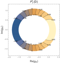
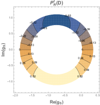
Figure 4: Average tauonic polarisations $P_{L,N,T}^{\tau}(D)$ for the allowed parameter space.

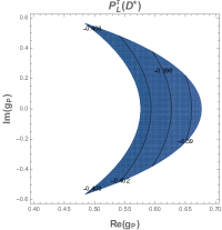
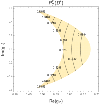
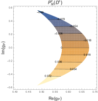
Figure 5: Average tauonic polarisations $P_{L,N,T}^{\tau}(D^{*})$ for the allowed parameter space.

3.4 $\Lambda_{b}\rightarrow\Lambda_{c}l\bar{\nu}$ decays

As mentioned in the introduction, there is one more ratio in the $b\to c\tau\nu$ family that is expected to be measured soon by LHCb, namely $\mathcal{R}(\Lambda_{c})$. In terms of the CCQM form factors we show the differential decay rate [69, 67] in the appendix.

From the partial decay width Eq.(52), we first obtain the $\Lambda_{b}\to\Lambda_{c}\mu\bar{\nu}_{\mu}$ normalised spectral distribution for the SM and compare it with the one measured by LHCb [70] in Figure 6. The green and yellow shaded areas indicate the estimated 10% and 20% errors in the prediction according to [64]. Once again, this figure serves to calibrate the performance of the CCQM form factors in this case.

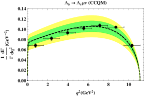
Figure 6: Normalised distribution $d\Gamma(\Lambda_{b}\to\Lambda_{c}\mu\bar{\nu}_{\mu})/(\Gamma dq^{2})$ with the CCQM form factors. The points are the LHCb data [70] and the dashed black line, green and yellow areas mark the central CCQM results and a 10% and 20% deviation respectively.

We also find in this case that the spectral distribution with new $g_{S,P}$ couplings constrained as above, cannot differentiate between the models. We turn to a prediction for $\mathcal{R}(\Lambda_{c})$ which is defined analogously to the previous ratios,

$$\mathcal{R}(\Lambda_{c})\equiv\frac{\Gamma(\Lambda_{b}\to\Lambda_{c}\tau\bar{\nu})}{\Gamma(\Lambda_{b}\to\Lambda_{c}l\bar{\nu})}, r(\Lambda_{c})=\frac{\mathcal{R}(\Lambda_{c})}{\mathcal{R}(\Lambda_{c})_{SM}}.$$ (16)

With the form factors in the appendix this leads to

$$r(\Lambda_{c})\approx\left(1+0.08\text{Re}[g_{P}]+0.43\text{Re}[g_{S}]+0.03|g_{P}|^{2}+0.33|g_{S}|^{2}\right).$$ (17)

It also leads to $\mathcal{R}(\Lambda_{c})_{SM}=0.295$, which compares well with other values found in the literature $\mathcal{R}(\Lambda_{c})_{SM}=0.33\pm 0.01$ [69]. Figure 7 shows $\mathcal{R}(\Lambda_{c})$ with new contributions from $g_{S}$ or $g_{P}$ in their allowed ranges. As Eq. 17 shows no interference between $g_{S}$ and $g_{P}$, the two new contributions simply add.

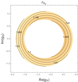
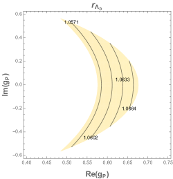
Figure 7: Predictions for $r_{(}\Lambda_{c})$ compatible with the measured $\mathcal{R}(D^{\star})$ at $2\sigma$ as well as ${\mathcal{B}}(B_{c}\to\tau\nu)\leq 30\%$. The left and right panels show separately the contributions from $g_{S}$ and $g_{P}$.

4 General two Higgs doublet model

The most general 2HDM-III, unlike the type I and type II more common versions, allows flavour changing neutral currents (FCNC) at tree-level which are then suppressed with family symmetries, minimal flavour violation, or specific patterns for the Yukawa couplings, for example. The most general renormaliseable quartic scalar potential is commonly written as [71],

$$V(\Phi_{1},\Phi_{2}) = \mu_{1}^{2}(\Phi_{1}^{{\dagger}}\Phi_{1})+\mu_{2}^{2}(\Phi_{2}^{{\dagger}}\Phi_{2})-\left(\mu_{12}^{2}(\Phi_{1}^{{\dagger}}\Phi_{2})+h.c\right)$$ (18)

$$+ \frac{1}{2}\lambda_{1}(\Phi_{1}^{{\dagger}}\Phi_{1})^{2}+\frac{1}{2}\lambda_{2}(\Phi_{2}^{{\dagger}}\Phi_{2})^{2}+\lambda_{3}(\Phi_{1}^{{\dagger}}\Phi_{1})(\Phi_{2}^{{\dagger}}\,\Phi_{2})+\lambda_{4}(\Phi_{1}^{{\dagger}}\Phi_{2})(\Phi_{2}^{{\dagger}}\Phi_{1})$$

$$+ \left(\frac{1}{2}\lambda_{5}(\Phi_{1}^{{\dagger}}\Phi_{2})^{2}+\left(\lambda_{6}(\Phi_{1}^{{\dagger}}\Phi_{1})+\lambda_{7}(\Phi_{2}^{{\dagger}}\Phi_{2})\right)(\Phi_{1}^{{\dagger}}\Phi_{2})+{\rm~{}h.c.}\right)$$

where the two scalar doublets are

$$\Phi_{i}=\left(\begin{array}[]{c}\phi_{i}^{+}\\ \frac{1}{\sqrt{2}}(\upsilon_{i}+\xi_{i}+i\zeta_{i})\end{array}\right).$$ (19)

Discrete symmetries in 2HDM type I and II force the parameters $\mu_{12}$ and $\lambda_{6,7}$ to vanish. The charged Higgs bosons that appear in the mass eigenstate basis correspond to the combinations

$$H^{\pm}=-s_{\beta}\phi_{1}^{\pm}+c_{\beta}\phi_{2}^{\pm}$$ (20)

with the rotation angle given by $\tan\beta=t_{\beta}=\frac{s_{\beta}}{c_{\beta}}=\frac{\upsilon_{2}}{\upsilon_{1}}$ and $\upsilon_{2}^{2}+\upsilon_{1}^{2}=\upsilon^{2}$ with $\upsilon=246$ GeV. There are three neutral scalars that are not CP eigenstates as the parameters $\mu_{12}$ and $\lambda_{6,7}$ can be complex and violate CP. These, however, will not play any role in our discussion beyond the occasional use of existing constraints on the mixing amongst the neutral scalars.

The most general Yukawa Lagrangian in the 2HDM-III without discrete symmetries is given by

$$\mathcal{L}_{Y}=-\left(\overline{Q}_{L}Y_{1}^{u}u_{R}\widetilde{\Phi}_{1}+\overline{Q}_{L}Y_{2}^{u}u_{R}\widetilde{\Phi}_{2}+\overline{Q}_{L}Y_{1}^{d}d_{R}\Phi_{1}\right.$$

$$+\left.\overline{Q}_{L}Y_{2}^{d}d_{R}\Phi_{2}+\overline{L}_{L}Y_{1}^{l}l_{R}\Phi_{1}+\overline{L}_{L}Y_{2}^{l}l_{R}\Phi_{2}\right)+{\rm~{}h.c.}$$ (21)

where $\widetilde{\Phi}_{1,2}=i\sigma_{2}\Phi_{1,2}^{*}$, $Q_{L}$ and $L_{L}$ denote the left-handed quark and lepton doublets, $u_{R}$, $d_{R}$ and $l_{R}$ the right-handed quark and lepton singlets and $Y_{1,2}^{u,d,l}$ denote the $(3\times 3)$ Yukawa matrices.

After spontaneous EWSB and in the fermion mass basis, the charged Higgs couplings to fermions can be written as:

$${\cal L}^{\bar{f}_{i}f_{j}\phi} = -\frac{g}{2\sqrt{2}M_{W}}\Bigg{[}\sum_{l=1}^{3}\bar{u}_{i}\Bigg{[}(V_{{\rm CKM}})_{il}\left(X\,m_{d_{l}}\,\delta_{lj}-\frac{f(X)}{\sqrt{2}}\,\sqrt{m_{d_{l}}m_{d_{j}}}\,\tilde{\chi}_{lj}^{d}\right)(1+\gamma^{5})$$

$$+\left(Y\,m_{u_{i}}\,\delta_{il}-\frac{f(Y)}{\sqrt{2}}\,\sqrt{m_{u_{i}}m_{u_{l}}}\,\tilde{\chi}_{il}^{u}\right)(V_{{\rm CKM}})_{lj}(1-\gamma^{5})\Bigg{]}\,d_{j}\,H^{+}$$

$$+\bar{\nu}_{i}\bigg{(}Z\,m_{l_{i}}\,\delta_{ij}-\frac{f(Z)}{\sqrt{2}}\,\sqrt{m_{l_{i}}m_{l_{j}}}\,\tilde{\chi}_{ij}^{l}\bigg{)}(1+\gamma^{5}){l}_{j}H^{+}+{\rm~{}h.c.}\Bigg{]}$$

where $f(x)=\sqrt{1+x^{2}}$. This form follows the notation of Refs. [72, 73, 74] in which the first term in each line in Eq. 4 is the coupling in one of the four 2HDM without FCNC and the second term is a flavour changing correction that makes it a type III model. Furthermore, the Cheng-Sher ansatz [75] has been implemented to control the size of the FCNC, but also allowing a CP violating phase:

$$\left[\tilde{Y}^{q,l}\right]_{ij}=\frac{\sqrt{m_{i}^{q,l}m_{j}^{q,l}}}{\upsilon}\,\left[\tilde{\chi}^{q,l}\right]_{ij}$$ (23)

with $\tilde{Y}^{f}=V_{fL}^{\dagger}Y^{f}V_{fR}$. The additional parameters that occur as a consequence of allowing flavour changing couplings are $\tilde{\chi}^{q.l}_{ij}$.

The parameters $X$, $Y$ and $Z$ given in Table 1 are the ones that occur in each of the four types of 2HDM with natural flavour conservation.

2HDM-III	$X$	$Y$	$Z$
Model I	$-\cot\beta$	$\cot\beta$	$-\cot\beta$
Model II	$\tan\beta$	$\cot\beta$	$\tan\beta$
Model X	$-\cot\beta$	$\cot\beta$	$\tan\beta$
Model Y	$\tan\beta$	$\cot\beta$	$-\cot\beta$

Table 1: Parameters $X$, $Y$ and $Z$ defined in the Yukawa interactions of Eq.(4) for four versions of the 2HDM-III.

We now turn to the question of the scalar coefficients in Eq. 8 within the. context of the 2HDM-III considered here. Tree-level exchange of the charged Higgs produces

$$C_{L}^{cb}=\frac{-1}{m_{H^{\pm}}^{2}}\Gamma_{cb}^{L}\Gamma_{\nu\tau}^{R}, C_{R}^{cb}=\frac{-1}{m_{H^{\pm}}^{2}}\Gamma_{cb}^{R}\Gamma_{\nu\tau}^{R},$$ (24)

and Eq.(4) implies that,

$$\Gamma_{ij}^{L} = \frac{g}{\sqrt{2}M_{W}}\sum_{l=1}^{3}\left(Y\,m_{u_{i}}\,\delta_{il}-\frac{f(Y)}{\sqrt{2}}\,\sqrt{m_{u_{i}}m_{u_{l}}}\,\tilde{\chi}_{il}^{u}\right)(V_{{\rm CKM}})_{lj},$$

$$\Gamma_{ij}^{R} = \frac{g}{\sqrt{2}M_{W}}\sum_{l=1}^{3}(V_{{\rm CKM}})_{il}\left(X\,m_{d_{l}}\,\delta_{lj}-\frac{f(X)}{\sqrt{2}}\,\sqrt{m_{d_{l}}m_{d_{j}}}\,\tilde{\chi}_{lj}^{d}\right),$$

$$\Gamma_{\nu_{i}j}^{R} = \frac{g}{\sqrt{2}M_{W}}\sum_{i=1}^{3}\bigg{(}Z\,m_{l_{i}}\,\delta_{ij}-\frac{f(Z)}{\sqrt{2}}\,\sqrt{m_{l_{i}}m_{l_{j}}}\,\tilde{\chi}_{ij}^{l}\bigg{)}.$$ (25)

Assuming that the parameters $\tilde{\chi}_{i,j}^{u}$ are of the same order and that the $\tilde{\chi}_{i,j}^{d}$ are also of the same order, as we expect in the context of the Cheng-Sher ansatz, the contributions from the heaviest fermions dominate the sums and Eq. 25 reduces to

$$\Gamma_{cb}^{L}\simeq\frac{g}{\sqrt{2}M_{W}}m_{c}V_{cb}\tilde{Y}, \tilde{Y}=\left(Y\,-\frac{V_{tb}}{V_{cb}}\frac{f(Y)}{\sqrt{2}}\,\sqrt{\frac{m_{t}}{m_{c}}}\,\tilde{\chi}_{ct}^{u}\right),$$

$$\Gamma_{cb}^{R}\simeq\frac{g}{\sqrt{2}M_{W}}m_{b}V_{cb}\tilde{X}, \tilde{X}=\left(X\,-\frac{V_{cs}}{V_{cb}}\frac{f(X)}{\sqrt{2}}\,\sqrt{\frac{m_{s}}{m_{b}}}\,\tilde{\chi}_{sb}^{d}\right),$$

$$\Gamma_{\nu\tau}^{R}\simeq\frac{g}{\sqrt{2}M_{W}}m_{\tau}\tilde{Z}, \tilde{Z}=\left(Z-\frac{f(Z)}{\sqrt{2}}\,\tilde{\chi}_{\tau\tau}^{l}\right).$$ (26)

The allowed parameter regions of Figure 1 then imply constraints on the parameters $m_{H^{\pm}},\,\tan\beta,\,\tilde{\chi}_{ij}^{u,d,l}$ which we discuss next in some detail. The general result is that it is possible to reach the allowed regions in Figure 1 with parameters of the model. Ref. [76] finds solutions for generalised models which can be written in terms of our Eqs. 26 with the factors $\tilde{X},\tilde{Y},\tilde{Z}$ being arbitrary parameters, independent of $\tan\beta$. The solutions they find occur for points with $\tilde{X}\sim{\cal O}(10)$, $\tilde{Y}\sim{\cal O}(100)$, $\tilde{Z}\sim{\cal O}(100)$ and $m_{H}<550$ GeV.

Once we allow for FCNC, all four cases of 2HDM-III can be mapped into the allowed regions in Figure 1. In Figures 8-11 we illustrate the results in two dimensional projections of parameter space. In all cases we present three figures. In the first one we consider the plane $\tan\beta-m_{H^{\pm}}$ and scan over all the real and imaginary parts of the $\tilde{\chi}$ parameters looking for points that satisfy the primary constraints ${\cal R}(D^{*})$ at $2\sigma$ and ${\mathcal{B}}(B_{c}\to\tau\nu)\leq 30\%$. In the second and third plots we illustrate regions of the parameter space of the $\tilde{\chi}$’s where the constraints are satisfied, in particular we specifically show solutions in the vicinity of $g_{s}=-0.5+0.7i$ and $g_{P}=0.63$ as these two points lie well inside the allowed regions of Figure 1. With solutions in this region of parameter space we find $\tilde{X},~{}\tilde{Y},~{}\tilde{Z}$ are ${\cal O}(10)$ to ${\cal O}(1000)$. It is important to emphasise, however, that these are only illustrations and that there are infinitely many solutions. Looking at the four models then,

• Model I. We present numerical results for this case in Figure 8. On the left panel we illustrate the region where solutions exist in the $\tan\beta-m_{H^{\pm}}$ plane. We see that a lower value of $\tan\beta$ and/or $m_{H^{\pm}}$ is needed to obtain solutions with smaller values of $|\tilde{\chi}^{u,d,l}|$. The region shown is dominated by low values of $\tan\beta$ which are compatible with constraints from LHC and LEP on the flavour conserving version of this model as seen in Figure 4 of Ref. [76]. Figure 9 of the same reference indicates that values of $\tan\beta\lesssim 2$ are ruled out by $B$ decay constraints. These constraints, however, can be significantly modified by flavour changing parameters such as $\tilde{\chi}^{d}_{bs}$. We are not aware of any global fit to the full set of parameters in the general 2HDM.

  

  

  

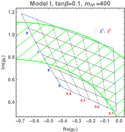
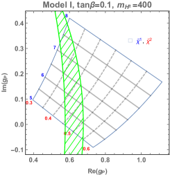
  Figure 8: Left panel: region where ${\cal R}(D^{(*)})$ agrees with experiment at $2\sigma$ and ${\mathcal{B}}(B_{c}\to\tau\nu)\leq 30\%$ in the $\tan\beta-m_{H^{\pm}}$ plane. Centre and right panels: we map solutions with $\tilde{\chi}^{d}_{sb}=\tilde{\chi}^{l}_{\tau\tau}=\tilde{\chi}^{1}e^{0.8i}$, $\tilde{\chi}^{u}_{ct}=\tilde{\chi}^{2}e^{2i}$, $\tan\beta=0.1$ and $m_{H^{\pm}}=400$ GeV onto the allowed regions of Figure 1 shown in green.

• Model II. We present numerical results for this case in Figure 9. On the left panel we illustrate the region where solutions exist in the $\tan\beta-m_{H^{\pm}}$ plane. We see that in this case a higher value of $\tan\beta$ and/or a lower value of $m_{H^{\pm}}$ is needed to obtain solutions with smaller values of $|\tilde{\chi}^{u,d,l}|$. The $\tan\beta-m_{H^{\pm}}$ region of solutions in this case is consistent with the constraints on the corresponding flavour conserving version of this model in Ref. [76]. The centre and right panels illustrate that solutions consistent with the Cheng-Sher ansatz exist in this case.

  

  

  

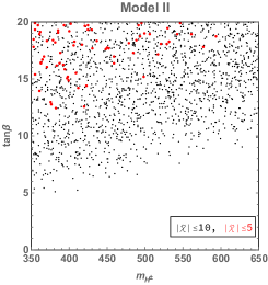
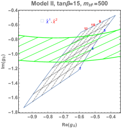
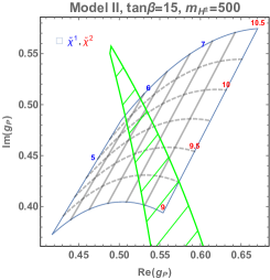
  Figure 9: Left panel: region where ${\cal R}(D^{(*)})$ agrees with experiment at $2\sigma$ and ${\mathcal{B}}(B_{c}\to\tau\nu)\leq 30\%$ in the $\tan\beta-m_{H^{\pm}}$ plane. Centre and right panels: we map solutions with $\tilde{\chi}^{d}_{sb}=\tilde{\chi}^{l}_{\tau\tau}=\tilde{\chi}^{1}e^{-0.8i}$, $\tilde{\chi}^{u}_{ct}=\tilde{\chi}^{2}e^{-1.2i}$, $\tan\beta=15$ and $m_{H^{\pm}}=500$ GeV onto the allowed regions of Figure 1 shown in green.

• Model X. We present numerical results for this case in Figure 10. On the left panel we illustrate the region where solutions exist in the $\tan\beta-m_{H^{\pm}}$ plane. We see that in this case a higher value of $\tan\beta$ and/or a lower value of $m_{H^{\pm}}$ is needed to obtain solutions with smaller values of $|\tilde{\chi}^{u,d,l}|$. This scenario is similar to Model II in that the $\tan\beta-m_{H^{\pm}}$ region of solutions is consistent with the constraints on its corresponding flavour conserving version as per Ref. [76] (called type IV in that reference). The region illustrated on the centre and right panels needs $|\chi^{d,l}|$ values larger than what the Cheng-Sher ansatz would suggest are natural. However, the left panel indicates that there are other solutions which are also consistent with this ansatz.

  

  

  

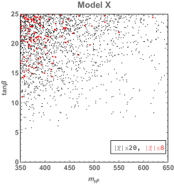
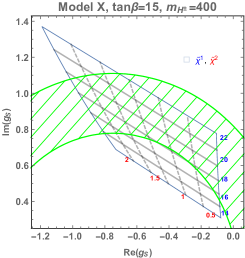
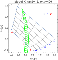
  Figure 10: Left panel: region where ${\cal R}(D^{(*)})$ agrees with experiment at $2\sigma$ and ${\mathcal{B}}(B_{c}\to\tau\nu)\leq 30\%$ in the $\tan\beta-m_{H^{\pm}}$ plane. Centre and right panel: we map solutions with $\tilde{\chi}^{d}_{sb}=\tilde{\chi}^{l}_{\tau\tau}=\tilde{\chi}^{1}e^{-2.4i}$, $\tilde{\chi}^{u}_{ct}=\tilde{\chi}^{2}e^{-1.2i}$, $\tan\beta=15$ and $m_{H^{\pm}}=400$ GeV onto the allowed regions of Figure 1 shown in green.

• Model Y. Finally, we present numerical results for this case in Figure 11. On the left panel we illustrate the region where solutions exist in the $\tan\beta-m_{H^{\pm}}$ plane. We see that in this case a higher value of $\tan\beta$ and/or a lower value of $m_{H^{\pm}}$ is needed to obtain solutions with smaller values of $|\tilde{\chi}^{u,d,l}|$. The $\tan\beta-m_{H^{\pm}}$ region of solutions is once again consistent with its corresponding flavour conserving version [76] (called type III in that reference), although the overlap region mostly lies in the upper range of both $\tan\beta$ and $m_{H^{\pm}}$ shown in the left panel. This panel also suggests that in this case, the $\tilde{\chi}$ parameters are required to be larger than expected in the Cheng-Sher ansatz.

  

  

  

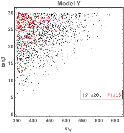
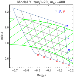
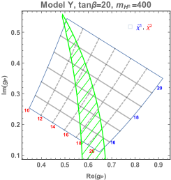
  Figure 11: Left panel: region where ${\cal R}(D^{(*)})$ agrees with experiment at $2\sigma$ and ${\mathcal{B}}(B_{c}\to\tau\nu)\leq 30\%$ in the $\tan\beta-m_{H^{\pm}}$ plane. Centre (right) panel: we map solutions with $\tilde{\chi}^{d}_{sb}=\tilde{\chi}^{l}_{\tau\tau}=\tilde{\chi}^{1}e^{0.7i}$, $\tilde{\chi}^{u}_{ct}=\tilde{\chi}^{2}e^{2i}$, $\tan\beta=20$ and $m_{H^{\pm}}=400$ GeV onto the allowed regions of Figure 1 shown in green.

Additional considerations that may restrict the parameters in the general model arise form Yukawa couplings to the neutral (SM-like) Higgs defined as

$$g_{hf_{i}f_{j}}=\frac{g}{2M_{W}}m_{f_{i}}h_{ij}^{f}.$$ (27)

Once we introduce non-zero couplings $\tilde{\chi}_{ct}^{u},\ \tilde{\chi}_{ct}^{u},\ \tilde{\chi}_{\tau\tau}^{l}$ as in Eq. 26, they also appear in $g_{h\tau\tau},\ g_{hct}$ and $g_{hsb}$, and are given by

$$h_{\tau\tau}^{l} = \begin{cases}\frac{\cos\alpha}{\sin\beta}+\frac{\cos(\beta-\alpha)}{\sin\beta}\frac{\tilde{\chi}_{\tau\tau}^{l}}{\sqrt{2}}&\mbox{for~{}models I, Y }\\ -\frac{\sin\alpha}{\cos\beta}+\frac{\cos(\beta-\alpha)}{\cos\beta}\frac{\tilde{\chi}_{\tau\tau}^{l}}{\sqrt{2}}&\mbox{for~{}models II, X}\end{cases}$$

$$h_{ct}^{u} = -\frac{\cos(\beta-\alpha)}{\sin\beta}\frac{\tilde{\chi}_{ct}^{u}}{\sqrt{2}}\sqrt{\frac{m_{t}}{m_{c}}}\ \mbox{for~{}all~{}models}$$

$$h_{sb}^{d} = \begin{cases}\frac{\cos(\beta-\alpha)}{\sin\beta}\frac{\tilde{\chi}_{sb}^{d}}{\sqrt{2}}\sqrt{\frac{m_{b}}{m_{s}}}&\mbox{for~{}models I, X }\\ \frac{\cos(\beta-\alpha)}{\cos\beta}\frac{\tilde{\chi}_{sb}^{d}}{\sqrt{2}}\sqrt{\frac{m_{b}}{m_{s}}}&\mbox{for~{}models II, Y}\end{cases}$$ (28)

These expressions simplify in the alignment limit, defined as $\cos(\beta-\alpha)\to 0$, in which case the couplings of $h$ tend to the SM Higgs couplings. To linear order in $\cos(\beta-\alpha)$ we obtain

$$|h_{\tau\tau}^{l}|^{2}-1 \approx \begin{cases}-2\cos(\beta-\alpha)\left(\cot\beta+\frac{\tilde{\chi}_{\tau\tau}^{l}}{\sqrt{2}\sin\beta}\right)&\mbox{for~{}models I, Y }\\ 2\cos(\beta-\alpha)\left(\tan\beta-\frac{\tilde{\chi}_{\tau\tau}^{l}}{\sqrt{2}\cos\beta}\right)&\mbox{for~{}models II, X}\end{cases}$$ (29)

The first constraint arises from the process $h\rightarrow\tau^{+}\tau^{-}$, for which the measured signal strength is [77]

$$\mu_{\tau}\equiv\frac{{\cal B}(h\rightarrow\tau^{+}\tau^{-})}{{\cal B}(h\rightarrow\tau^{+}\tau^{-})_{SM}}=1.11_{-0.22}^{+0.24},$$ (30)

leads to

$$-0.32\lesssim|h_{\tau\tau}^{l}|^{2}-1\lesssim 0.58$$ (31)

at the 95% confidence level.

In addition, if the flavour changing couplings get too large they will conflict with the non-observation of $t\to ch$ and with indirect limits on $h\to bs$. For $\mathcal{B}(t\to hc)<0.22\%$ at 95% c.l. [78] one finds

$$\left|\frac{\cos(\beta-\alpha)}{\sin\beta}\tilde{\chi}_{ct}^{u}\right|\lesssim 1.4.$$ (32)

The process $h\to bs$ has not been constrained yet, but it has been argued in the literature that a branching ratio as large as $\mathcal{B}(h\to bs)\sim 36\%$ can remain consistent with other flavour results in these types of models [79]. Adopting this number and with the 95% c. l. $\Gamma_{H}<0.013$ GeV [78] we find,

$$|\frac{\cos(\beta-\alpha)}{\sin\beta}\tilde{\chi}_{sb}^{d}|\lesssim 17\ \ \mbox{for~{}models I, X},$$

$$|\frac{\cos(\beta-\alpha)}{\cos\beta}\tilde{\chi}_{sb}^{d}|\lesssim 17\ \ \mbox{for~{}models II, Y}.$$ (33)

The constraints in Eqs. 31-33 depend on $\cos(\beta-\alpha)$ and disappear in the alignment limit. Ref. [80] presents upper bounds on $\cos(\beta-\alpha)$ of ${\cal O}(0.1)$ that depend on $\tan\beta$ for the four types of flavor conserving models, so they do not automatically extend to our case.

5 Summary Conclusions

We have revisited the 2HDM-III as a possible explanation for the $\mathcal{R}(D^{(*)})$ anomalies. We first summarised the constraints known in the literature in terms of generic (pseudo)-scalar couplings and discussed the possible conflict between $\mathcal{R}(D^{*})$ and ${\mathcal{B}}(B_{c}\to\tau\nu)\leq 30\%$. We found that the parameter space that can explain these two anomalies at the two-sigma level is limited to the region ${\mathcal{B}}(B_{c}\to\tau\nu)>23\%$. The bound ${\mathcal{B}}(B_{c}\to\tau\nu)>10\%$ advocated in Ref.[60] in turn restricts the possible explanation of $\mathcal{R}(D^{(*)})$ to the $3\sigma$ level within these models.

Armed with these constraints we predicted the ranges of other observables in $b\to c\tau\nu$ reactions, including $\mathcal{R}(J/\psi)$ and $\mathcal{R}(\Lambda_{c})$. We find that the large central value in the current measurement of $\mathcal{R}(J/\psi)$ is consistent with this model at about the $2\sigma$ level with the currently large experimental error, but that a more precise measurement of this quantity could place it in conflict with $\mathcal{R}(D^{(*)})$.

We found that the distributions $d\Gamma/dq^{2}$ in $B\to D\tau\nu$, $B\to D^{(*)}\tau\nu$ or $B_{c}\to J/\psi\tau\nu$ cannot distinguish between the SM or models with new (pseudo)-scalar couplings.

We presented predictions for the tau-lepton polarisation in $B\to D^{(*)}\tau\nu$ in the presently allowed region of parameter space. In particular we find that phases in the Yukawa couplings can produce substantial T-odd normal polarisations.

We considered four versions of the 2HDM-III which are constructed by extending the four flavour conserving 2HDM with the addition of flavour changing couplings that we have limited in size with the Sher-Cheng ansatz. We mapped the allowed regions in $g_{P}-g_{S}$ into the parameter space of these four models. We found that the allowed $(m_{H^{\pm}},\tan\beta)$ ranges also satisfy the LHC and LEP constraints found in the literature for the flavour conserving versions of these models. We also found that the allowed regions of parameter space are not further constrained by $h\to\tau\tau$, $t\to hc$, $h\to bs$.

Appendix A Helicity Amplitudes

The invariant form factors describing the hadronic transitions $\bar{B}\to D$ and $\overline{B}\to D^{*}$ are defined as usual

$$\langle D(p_{2})|\bar{c}\gamma^{\mu}b|\bar{B}(p_{1})\rangle=F_{+}(q^{2})P^{\mu}+F_{-}(q^{2})q^{\mu},$$

$$\langle D(p_{2})|\bar{c}b|\bar{B}(p_{1})\rangle=(m1+m2)F^{S}(q^{2}),$$

$$\langle D^{*}(p_{2})|\bar{c}\gamma^{\mu}(1\mp\gamma^{5})b|\bar{B}(p_{1})\rangle=\frac{\epsilon_{2\alpha}^{\dagger}}{m_{1}+m_{2}}\Big{[}\mp g^{\mu\alpha}PqA_{0}(q^{2})$$

$$\pm P^{\mu}P^{\alpha}A_{+}(q^{2})\pm q^{\mu}P^{\alpha}A_{-}(q^{2})+i\varepsilon^{\mu\alpha}PqV(q^{2})\Big{]},$$

$$\langle D^{*}(p_{2})|\bar{c}\gamma^{5}b|\bar{B}(p_{1})\rangle=\epsilon_{2\alpha}^{\dagger}P^{\alpha}G^{S}(q^{2}),$$ (34)

where $P=p_{1}+p_{2}$, $q=p_{1}-p_{2}$, and $\epsilon_{2}$ is the polarization vector of the $D^{*}$ meson which satisfies $\epsilon_{2}^{\dagger}\cdot p_{2}=0$. The particles are on their mass shells: $p_{1}^{2}=m_{B}^{2}$ and $p_{2}^{2}=m_{D^{(\ast)}}^{2}$. All the expressions are written in terms of helicity form factors, which are related to those in Eq. 34 for the $\overline{B}\to D$ transition by [64]

$$H_{t} = \frac{PqF_{+}+q^{2}F_{-}}{\sqrt{q^{2}}},\,$$ (35)

$$H_{0} = \frac{2m_{B}|\mathbf{p_{2}|}F_{+}}{\sqrt{q^{2}}},$$ (36)

$$H_{P}^{S} = (m_{B}+m_{D})F^{S},$$ (37)

where $|{\bf p_{2}}|=\lambda^{1/2}(m_{B}^{2},m_{D^{(*)}}^{2},q^{2})/2m_{B}$ is the momentum of the daughter meson with $\lambda=(m_{B}^{2}-m_{D^{(*)}}^{2}-q^{2})^{2}-4m_{D^{(*)}}^{2}q^{2}.$ For the $\overline{B}\to D^{*}$ transition [64]

$$H_{t} = \frac{m_{B}|{\bf p_{2}}|\left(Pq(-A_{0}+A_{+})+q^{2}A_{-}\right)}{m_{D^{*}}\sqrt{q^{2}}(m_{B}+m_{D^{*}})},$$ (38)

$$H_{\pm} = \frac{-PqA_{0}\pm 2m_{1}|{\bf p_{2}}|V}{m_{B}+m_{D^{*}}},$$ (39)

$$H_{V}^{S} = \frac{m_{B}}{m_{D^{*}}}|{\bf p_{2}}|G^{S},$$ (40)

$$H_{0} = \frac{-Pq(m_{B}^{2}-m_{D^{*}}^{2}-q^{2})A_{0}+4m_{B}^{2}|{\bf p_{2}}|^{2}A_{+}}{2m_{2}\sqrt{q^{2}}(m_{B}+m_{D^{*}})}.$$ (41)

For our numerical estimates we use the helicity amplitudes calculated in the covariant confined quark model (CCQM) with the double-pole parameterisation of Refs. [64, 66]:

$$j(q^{2}) = \frac{j(0)}{1-a_{j}s+b_{j}s^{2}},\quad s=\frac{q^{2}}{m_{B}^{2}},$$ (42)

$$j=F_{\pm},\,A_{0,\pm},\,F^{S},\,G^{S},\,V.$$

Similarly, for the $\Lambda_{b}$ decay we need the vector and axial current form factors [69, 81]

$$H_{\lambda_{2},\lambda_{W}}=H_{\lambda_{2},\lambda_{W}}^{V}-H_{\lambda_{2},\lambda_{W}}^{A},$$ (43)

$$H_{\lambda_{2},\lambda_{W}}^{V(A)}=\epsilon^{\dagger\mu}(\lambda_{W})\langle\Lambda_{c},\lambda_{2}|\bar{c}\gamma_{\mu}(\gamma_{\mu}\gamma_{5})b|\Lambda_{b},\lambda_{1}\rangle,$$ (44)

which satisfy the parity relations,

$$H_{\lambda_{2},\lambda_{W}}^{V}=H_{-\lambda_{2},-\lambda_{W}}^{V},\quad H_{\lambda_{2},\lambda_{W}}^{A}=-H_{-\lambda_{2},-\lambda_{W}}^{A},$$ (45)

$$H_{-\lambda_{2},-\lambda_{W}}=H_{\lambda_{2},\lambda_{W}}^{V}+H_{\lambda_{2},\lambda_{W}}^{A},$$ (46)

where $\lambda_{2}$ and $\lambda_{W}$ denote the helicities of the daughter baryon $\Lambda_{c}$ and the virtual $W$ boson respectively. In the SM the helicity amplitudes $H_{\lambda_{2},\lambda_{W}}^{V(A)}$are given by [81]

$$H_{+\frac{1}{2},t}^{V(A)} =\sqrt{\frac{Q_{\pm}}{q^{2}}}\left(M_{\mp}F_{1}^{V(A)}\pm\frac{q^{2}}{M_{\Lambda_{b}}}F_{3}^{V(A)}\right),$$ (47)

$$H_{+\frac{1}{2},+}^{V(A)} =\sqrt{2Q_{\mp}}\left(F_{1}^{V(A)}\pm\frac{M_{\pm}}{M_{\Lambda_{b}}}F_{2}^{V(A)}\right),$$ (48)

$$H_{+\frac{1}{2},0}^{V(A)} =\sqrt{\frac{Q_{\mp}}{q^{2}}}\left(M_{\pm}F_{1}^{V(A)}\pm\frac{q^{2}}{M_{\Lambda_{b}}}F_{2}^{V(A)}\right).$$ (49)

with $M_{\pm}=M_{\Lambda_{b}}\pm M_{\Lambda_{c}}$ and $Q_{\pm}=M_{\pm}^{2}-q^{2}$. The helicity amplitudes for scalar and pseudo-scalar operators needed for 2HDM are [67]

$$H_{\lambda_{2},0}^{SP}= H_{\lambda_{2},0}^{S}-H_{\lambda_{2},0}^{P},$$ (50)

$$H_{\pm\frac{1}{2},0}^{SP}= \frac{\sqrt{Q_{+}}}{m_{b}-m_{c}}\left(M_{-}F_{1}^{V}+\frac{q^{2}}{M_{\Lambda_{b}}}F_{3}^{V}\right)$$

$$\pm\frac{\sqrt{Q_{-}}}{m_{b}+m_{c}}\left(M_{+}F_{1}^{A}-\frac{q^{2}}{M_{\Lambda_{b}}}F_{3}^{A}\right).$$ (51)

In this way, the partial decay width of the $\Lambda_{b}\to\Lambda_{c}l\bar{\nu}$ process is given by [67]

$$\frac{{\rm d}\Gamma}{{\rm d}q^{2}}=\frac{G_{F}^{2}|V_{cb}|^{2}q^{2}|\vec{\mathbf{p}}_{2}|}{192\pi{}^{3}M_{\Lambda_{b}}^{2}}\left(1-2\delta_{l}\right)^{2}\left[\left(1+\delta_{l}\right)\sum_{ij}H_{ij}^{2}+\frac{3}{2}B_{3}^{NP}+\frac{3m_{l}}{\sqrt{q^{2}}}B_{4}^{Int}\right]$$ (52)

where $\delta_{l}=m_{l}^{2}/2q^{2}$, $ij=(-\frac{1}{2},-),\,(-\frac{1}{2},0),\,(\frac{1}{2},0),\,(\frac{1}{2},+)$ and

$$B_{3}^{NP} = |H_{1/2,0}^{SP}|^{2}+|H_{-1/2,0}^{SP}|^{2},$$

$$B_{4}^{Int} = \mathrm{Re}(H_{1/2,t}\ (H_{1/2,0}^{SP})^{*}+H_{-1/2,t}\ (H_{-1/2,0}^{SP})^{*}).$$ (53)

Appendix B Polarisations

Following Ref. [64], the ratios ${\cal R}(D^{(*)})$ are given by

$$\mathcal{R}(D^{(*)})=\frac{\left(\frac{q^{2}-m_{\tau}^{2}}{q^{2}-m_{\mu}^{2}}\right){\cal H}_{tot}(D^{(*)})}{\sum_{n}|H_{n}|^{2}+\delta_{\mu}\big{(}\sum_{n}|H_{n}|^{2}+3|H_{t}|^{2}\big{)}},$$ (54)

with

$${\cal H}_{tot}(D) =\left[|H_{0}|^{2}+\delta_{\tau}(|H_{0}|^{2}+3|H_{t}|^{2}\right]+\frac{3}{2}|g_{S}|^{2}|H_{P}^{S}|^{2}+3\sqrt{2\delta_{\tau}}\textrm{Re[}g_{S}]H_{P}^{S}H_{t},$$

$${\cal H}_{tot}(D^{*}) =\sum_{n}|H_{n}|^{2}\left(\delta_{\tau}+1\right)+3\delta_{\tau}|H_{t}|^{2}+\frac{3}{2}|g_{P}|^{2}|H_{V}^{S}|^{2}-3\sqrt{2\delta_{\tau}}\textrm{Re[}g_{P}]H_{V}^{S}H_{t},$$ (55)

and $g_{S}\equiv\left(C_{L}^{cb}+C_{R}^{cb}\right)/C_{SM}^{cb}$ and $g_{P}\equiv\left(C_{L}^{cb}-C_{R}^{cb}\right)/C_{SM}^{cb}$. In terms of Eq. 55, the longitudinal differential polarisation will be,

$${\cal H}_{tot}(D)\frac{dP_{L}^{\tau}(D)}{dq^{2}} = \left[|H_{0}|^{2}\left(\delta_{\tau}-1\right)+3\delta_{\tau}|H_{t}|^{2}+\frac{3}{2}|g_{S}|^{2}|H_{P}^{S}|^{2}+3\sqrt{2\delta_{\tau}}\textrm{Re(}g_{S})H_{P}^{S}H_{t}\right],$$ (56)

$${\cal H}_{tot}(D^{*})\frac{dP_{L}^{\tau}(D^{*})}{dq^{2}} = \left[\sum_{n}|H_{n}|^{2}\left(\delta_{\tau}-1\right)+3\delta_{\tau}|H_{t}|^{2}+\frac{3}{2}|g_{P}|^{2}|H_{V}^{S}|^{2}-3\sqrt{2\delta_{\tau}}\textrm{Re(}g_{P})H_{V}^{S}H_{t}\right].$$

Similarly, the transverse polarisation is given by

$$\frac{dP_{T}^{\tau}(D)}{dq^{2}} = \frac{3\pi\sqrt{\delta_{\tau}}}{2\sqrt{2}{\cal H}_{tot}(D)}\left(H_{0}H_{t}+\frac{\textrm{Re(}g_{S})H_{P}^{S}H_{0}}{\sqrt{2\delta_{\tau}}}\right),$$

$$\frac{dP_{T}^{\tau}(D^{*})}{dq^{2}} = \frac{3\pi\sqrt{\delta_{\tau}}}{4\sqrt{2}{\cal H}_{tot}(D^{*})}\left[\left(|H_{-}|^{2}-|H_{+}|^{2}\right)+2H_{0}H_{t}-\frac{2\textrm{Re}(g_{P})H_{V}^{S}H_{0}}{\sqrt{2\delta_{\tau}}}\right].$$ (57)

Finally, in the presence of CP-violating phases in the NP Higgs exchange amplitude, there is a normal differential polarisation that reads

$$\frac{dP_{N}^{\tau}(D)}{dq^{2}} = \frac{-3\pi}{4{\cal H}_{tot}(D)}\textrm{Im(}g_{S})H_{P}^{S}H_{0},$$

$$\frac{dP_{N}^{\tau}(D^{*})}{dq^{2}} = \frac{3\pi}{4{\cal H}_{tot}(D^{*})}\textrm{Im(}g_{P})H_{V}^{S}H_{0}.$$ (58)

To calculate the integrated, or $q^{2}$ averaged polarisations, one has to include the $q^{2}$-dependent phase-space factor $C(q^{2})=|\mathbf{p_{2}}|(q^{2}-m_{\tau}^{2})^{2}/q^{2}$ [64],

$$P_{i}^{\tau}(D^{(*)})=\frac{\intop_{m_{\tau}^{2}}^{q_{max}^{2}}dq^{2}C(q^{2})\frac{dP_{i}^{\tau}(D^{(*)})}{dq^{2}}{\cal H}_{tot}(D^{(*)})}{\intop_{m_{\tau}^{2}}^{q_{max}^{2}}dq^{2}C(q^{2}){\cal H}_{tot}(D^{(*)})}.$$ (59)

References

• [1] BaBar collaboration, J. P. Lees et al., Evidence for an excess of $\bar{B}\to D^{(*)}\tau^{-}\bar{\nu}_{\tau}$ decays, Phys. Rev. Lett. 109 (2012) 101802, [1205.5442].
• [2] BaBar collaboration, J. P. Lees et al., Measurement of an Excess of $\bar{B}\to D^{(*)}\tau^{-}\bar{\nu}_{\tau}$ Decays and Implications for Charged Higgs Bosons, Phys. Rev. D88 (2013) 072012, [1303.0571].
• [3] Belle collaboration, M. Huschle et al., Measurement of the branching ratio of $\bar{B}\to D^{(\ast)}\tau^{-}\bar{\nu}_{\tau}$ relative to $\bar{B}\to D^{(\ast)}\ell^{-}\bar{\nu}_{\ell}$ decays with hadronic tagging at Belle, Phys. Rev. D92 (2015) 072014, [1507.03233].
• [4] Belle collaboration, Y. Sato et al., Measurement of the branching ratio of $\bar{B}^{0}\rightarrow D^{*+}\tau^{-}\bar{\nu}_{\tau}$ relative to $\bar{B}^{0}\rightarrow D^{*+}\ell^{-}\bar{\nu}_{\ell}$ decays with a semileptonic tagging method, Phys. Rev. D94 (2016) 072007, [1607.07923].
• [5] Belle collaboration, S. Hirose et al., Measurement of the $\tau$ lepton polarization and $R(D^{*})$ in the decay $\bar{B}\to D^{*}\tau^{-}\bar{\nu}_{\tau}$, Phys. Rev. Lett. 118 (2017) 211801, [1612.00529].
• [6] LHCb collaboration, R. Aaij et al., Measurement of the ratio of branching fractions $\mathcal{B}(\bar{B}^{0}\to D^{*+}\tau^{-}\bar{\nu}_{\tau})/\mathcal{B}(\bar{B}^{0}\to D^{*+}\mu^{-}\bar{\nu}_{\mu})$, Phys. Rev. Lett. 115 (2015) 111803, [1506.08614].
• [7] BaBar, LHCb collaboration, G. Wormser, Measurement of the ratio of branching fractions $\cal{B}(B^{0}\to D^{*-}\tau^{+}\nu_{\tau})/\cal{B}(B^{0}\to D^{*-}\mu^{+}\nu_{\mu})$ with hadronic $\tau$ three-prong decays, PoS FPCP2017 (2017) 006.
• [8] HFLAV collaboration, Y. Amhis et al., Averages of $b$-hadron, $c$-hadron, and $\tau$-lepton properties as of summer 2016, Eur. Phys. J. C77 (2017) 895, [1612.07233].
• [9] MILC collaboration, J. A. Bailey et al., $B\to D\ell\nu$ form factors at nonzero recoil and |Vcb| from 2+1-flavor lattice QCD, Phys. Rev. D92 (2015) 034506, [1503.07237].
• [10] HPQCD collaboration, H. Na, C. M. Bouchard, G. P. Lepage, C. Monahan and J. Shigemitsu, $B\rightarrow Dl\nu$ form factors at nonzero recoil and extraction of $|V_{cb}|$, Phys. Rev. D92 (2015) 054510, [1505.03925].
• [11] S. Fajfer, J. F. Kamenik and I. Nisandzic, On the $B\to D^{*}\tau\bar{\nu}_{\tau}$ Sensitivity to New Physics, Phys. Rev. D85 (2012) 094025, [1203.2654].
• [12] D. Bigi, P. Gambino and S. Schacht, $R(D^{*})$, $|V_{cb}|$, and the Heavy Quark Symmetry relations between form factors, JHEP 11 (2017) 061, [1707.09509].
• [13] LHCb collaboration, R. Aaij et al., Measurement of the ratio of branching fractions $\mathcal{B}(B_{c}^{+}\,\to\,J/\psi\tau^{+}\nu_{\tau})$/$\mathcal{B}(B_{c}^{+}\,\to\,J/\psi\mu^{+}\nu_{\mu})$, Phys. Rev. Lett. 120 (2018) 121801, [1711.05623].
• [14] A. Yu. Anisimov, I. M. Narodetsky, C. Semay and B. Silvestre-Brac, The $B_{c}$ meson lifetime in the light front constituent quark model, Phys. Lett. B452 (1999) 129–136, [hep-ph/9812514].
• [15] V. V. Kiselev, Exclusive decays and lifetime of $B_{c}$ meson in QCD sum rules, hep-ph/0211021.
• [16] M. A. Ivanov, J. G. Korner and P. Santorelli, Exclusive semileptonic and nonleptonic decays of the $B_{c}$ meson, Phys. Rev. D73 (2006) 054024, [hep-ph/0602050].
• [17] E. Hernandez, J. Nieves and J. M. Verde-Velasco, Study of exclusive semileptonic and non-leptonic decays of $B_{c}$ - in a nonrelativistic quark model, Phys. Rev. D74 (2006) 074008, [hep-ph/0607150].
• [18] R. Watanabe, New Physics effect on $B_{c}\to J/\psi\tau\bar{\nu}$ in relation to the $R_{D^{(*)}}$ anomaly, Phys. Lett. B776 (2018) 5–9, [1709.08644].
• [19] M. Tanaka and R. Watanabe, New physics in the weak interaction of $\bar{B}\to D^{(*)}\tau\bar{\nu}$, Phys. Rev. D87 (2013) 034028, [1212.1878].
• [20] G.-H. Wu, K. Kiers and J. N. Ng, Polarization measurements and T violation in exclusive semileptonic B decays, Phys. Rev. D56 (1997) 5413–5430, [hep-ph/9705293].
• [21] J.-P. Lee, CP violating transverse lepton polarization in B —> D(*) l anti-nu including tensor interactions, Phys. Lett. B526 (2002) 61–71, [hep-ph/0111184].
• [22] C.-H. Chen and C.-Q. Geng, Lepton angular asymmetries in semileptonic charmful B decays, Phys. Rev. D71 (2005) 077501, [hep-ph/0503123].
• [23] C.-H. Chen and T. Nomura, Charged-Higgs on $R_{D^{(*)}}$, $\tau$ polarization, and FBA, Eur. Phys. J. C77 (2017) 631, [1703.03646].
• [24] S. Iguro and Y. Omura, Status of the semileptonic $B$ decays and muon g-2 in general 2HDMs with right-handed neutrinos, JHEP 05 (2018) 173, [1802.01732].
• [25] J. F. Kamenik and F. Mescia, $B\to D\tau\nu$ Branching Ratios: Opportunity for Lattice QCD and Hadron Colliders, Phys. Rev. D78 (2008) 014003, [0802.3790].
• [26] M. Tanaka and R. Watanabe, Tau longitudinal polarization in $B\to D\tau\nu$ and its role in the search for charged Higgs boson, Phys. Rev. D82 (2010) 034027, [1005.4306].
• [27] A. Crivellin, C. Greub and A. Kokulu, Explaining $B\to D\tau\nu$, $B\to D^{*}\tau\nu$ and $B\to\tau\nu$ in a 2HDM of type III, Phys. Rev. D86 (2012) 054014, [1206.2634].
• [28] A. Celis, M. Jung, X.-Q. Li and A. Pich, Sensitivity to charged scalars in $\boldsymbol{B\to D^{(*)}\tau\nu_{\tau}}$ and $\boldsymbol{B\to\tau\nu_{\tau}}$ decays, JHEP 01 (2013) 054, [1210.8443].
• [29] N. G. Deshpande and A. Menon, Hints of R-parity violation in B decays into $\tau\nu$, JHEP 01 (2013) 025, [1208.4134].
• [30] S. Fajfer, J. F. Kamenik, I. Nisandzic and J. Zupan, Implications of Lepton Flavor Universality Violations in B Decays, Phys. Rev. Lett. 109 (2012) 161801, [1206.1872].
• [31] A. Datta, M. Duraisamy and D. Ghosh, Diagnosing New Physics in $b\to c\,\tau\,\nu_{\tau}$ decays in the light of the recent BaBar result, Phys. Rev. D86 (2012) 034027, [1206.3760].
• [32] D. Bečirević, N. KoÅ¡nik and A. Tayduganov, $\bar{B}\to D\tau\bar{\nu}_{\tau}$ vs. $\bar{B}\to D\mu\bar{\nu}_{\mu}$, Phys. Lett. B716 (2012) 208–213, [1206.4977].
• [33] X.-G. He and G. Valencia, $B$ decays with $\tau$ leptons in nonuniversal left-right models, Phys. Rev. D87 (2013) 014014, [1211.0348].
• [34] A. Rashed, M. Duraisamy and A. Datta, Nonstandard interactions of tau neutrino via charged Higgs and $W^{\prime}$ contribution, Phys. Rev. D87 (2013) 013002, [1204.2023].
• [35] Y. Sakaki and H. Tanaka, Constraints on the charged scalar effects using the forward-backward asymmetry on $B^{-}\to D(*)\tau\nu$ , Phys. Rev. D87 (2013) 054002, [1205.4908].
• [36] P. Ko, Y. Omura and C. Yu, $B\to D^{(}*)\tau\nu$ and $B\to\tau\nu$ in chiral U(1)’ models with flavored multi Higgs doublets, JHEP 03 (2013) 151, [1212.4607].
• [37] G. Bambhaniya, J. Chakrabortty, J. Gluza, M. Kordiaczyńska and R. Szafron, Left-Right Symmetry and the Charged Higgs Bosons at the LHC, JHEP 05 (2014) 033, [1311.4144].
• [38] M. Atoui, V. Morénas, D. Bečirevic and F. Sanfilippo, $B_{s}\to D_{s}\ell\nu_{\ell}$ near zero recoil in and beyond the Standard Model, Eur. Phys. J. C74 (2014) 2861, [1310.5238].
• [39] R. Dutta, A. Bhol and A. K. Giri, Effective theory approach to new physics in $b\to u$ and $b\to c$ leptonic and semileptonic decays, Phys. Rev. D88 (2013) 114023, [1307.6653].
• [40] M. Freytsis, Z. Ligeti and J. T. Ruderman, Flavor models for $\bar{B}\to D^{(*)}\tau\bar{\nu}$, Phys. Rev. D92 (2015) 054018, [1506.08896].
• [41] S. M. Boucenna, A. Celis, J. Fuentes-Martin, A. Vicente and J. Virto, Non-abelian gauge extensions for B-decay anomalies, Phys. Lett. B760 (2016) 214–219, [1604.03088].
• [42] S. M. Boucenna, A. Celis, J. Fuentes-Martin, A. Vicente and J. Virto, Phenomenology of an $SU(2)\times SU(2)\times U(1)$ model with lepton-flavour non-universality, JHEP 12 (2016) 059, [1608.01349].
• [43] C.-W. Chiang, X.-G. He and G. Valencia, $Z^{\prime}$ model for $b\to s\ell\bar{\ell}$ flavor anomalies, Phys. Rev. D93 (2016) 074003, [1601.07328].
• [44] J. Zhu, H.-M. Gan, R.-M. Wang, Y.-Y. Fan, Q. Chang and Y.-G. Xu, Probing the R-parity violating supersymmetric effects in the exclusive $b\to c\ell^{-}\bar{\nu}_{\ell}$ decays, Phys. Rev. D93 (2016) 094023, [1602.06491].
• [45] C. S. Kim, G. Lopez-Castro, S. L. Tostado and A. Vicente, Remarks on the Standard Model predictions for $R(D)$ and $R(D^{*})$, Phys. Rev. D95 (2017) 013003, [1610.04190].
• [46] A. Celis, M. Jung, X.-Q. Li and A. Pich, Scalar contributions to $b\to c(u)\tau\nu$ transitions, Phys. Lett. B771 (2017) 168–179, [1612.07757].
• [47] R. Dutta and A. Bhol, $B_{c}\to(J/\psi,\,\eta_{c})\tau\nu$ semileptonic decays within the standard model and beyond, Phys. Rev. D96 (2017) 076001, [1701.08598].
• [48] G. Cvetič, F. Halzen, C. S. Kim and S. Oh, Anomalies in (semi)-leptonic $B$ decays $B^{\pm}\to\tau^{\pm}\nu$, $B^{\pm}\to D\tau^{\pm}\nu$ and $B^{\pm}\to D^{*}\tau^{\pm}\nu$, and possible resolution with sterile neutrino, Chin. Phys. C41 (2017) 113102, [1702.04335].
• [49] P. Ko, Y. Omura, Y. Shigekami and C. Yu, LHCb anomaly and B physics in flavored $Z^{\prime}$ models with flavored Higgs doublets, Phys. Rev. D95 (2017) 115040, [1702.08666].
• [50] C.-H. Chen, T. Nomura and H. Okada, Excesses of muon $g-2$, $R_{D^{(\ast)}}$, and $R_{K}$ in a leptoquark model, Phys. Lett. B774 (2017) 456–464, [1703.03251].
• [51] R. Dutta, Exploring $R_{D}$, $R_{D^{\ast}}$ and $R_{J/\Psi}$ anomalies, 1710.00351.
• [52] X.-G. He and G. Valencia, Lepton universality violation and right-handed currents in $b\to c\tau\nu$, Phys. Lett. B779 (2018) 52–57, [1711.09525].
• [53] A. Greljo, D. J. Robinson, B. Shakya and J. Zupan, $R(D^{(*)})$ from $W^{\prime}$ and right-handed neutrinos, 1804.04642.
• [54] P. Asadi, M. R. Buckley and D. Shih, It’s all right(-handed neutrinos): a new $W^{\prime}$ model for the $R_{D^{(*)}}$ anomaly, 1804.04135.
• [55] J. M. Cline, Scalar doublet models confront $\tau$ and $b$ anomalies, Phys. Rev. D93 (2016) 075017, [1512.02210].
• [56] A. Crivellin, J. Heeck and P. Stoffer, A perturbed lepton-specific two-Higgs-doublet model facing experimental hints for physics beyond the Standard Model, Phys. Rev. Lett. 116 (2016) 081801, [1507.07567].
• [57] A. Crivellin, A. Kokulu and C. Greub, Flavor-phenomenology of two-Higgs-doublet models with generic Yukawa structure, Phys. Rev. D87 (2013) 094031, [1303.5877].
• [58] C.-H. Chen and T. Nomura, Charged-Higgs on $B^{-}_{q}\to\ell\bar{\nu}$ and $\bar{B}\to(P,V)\ell\bar{\nu}$ in a generic two-Higgs doublet model, 1803.00171.
• [59] R. Alonso, B. Grinstein and J. Martin Camalich, Lifetime of $B_{c}^{-}$ Constrains Explanations for Anomalies in $B\to D^{(*)}\tau\nu$, Phys. Rev. Lett. 118 (2017) 081802, [1611.06676].
• [60] A. G. Akeroyd and C.-H. Chen, Constraint on the branching ratio of $B_{c}\to\tau\bar{\nu}$ from LEP1 and consequences for $R(D^{(*)})$ anomaly, Phys. Rev. D96 (2017) 075011, [1708.04072].
• [61] E. Golowich and G. Valencia, Triple Product Correlations in Semileptonic $B^{\pm}$ Decays, Phys. Rev. D40 (1989) 112.
• [62] M. Tanaka, Charged Higgs effects on exclusive semitauonic $B$ decays, Z. Phys. C67 (1995) 321–326, [hep-ph/9411405].
• [63] K. Hagiwara, M. M. Nojiri and Y. Sakaki, $CP$ violation in $B\to D\tau\nu_{\tau}$ using multipion tau decays, Phys. Rev. D89 (2014) 094009, [1403.5892].
• [64] M. A. Ivanov, J. G. Körner and C.-T. Tran, Probing new physics in $\bar{B}^{0}\to D^{(\ast)}\tau^{-}\bar{\nu}_{\tau}$ using the longitudinal, transverse, and normal polarization components of the tau lepton, Phys. Rev. D95 (2017) 036021, [1701.02937].
• [65] R. Garisto, Cp violating polarizations in semileptonic heavy meson decays, Phys. Rev. D51 (1995) 1107–1116, [hep-ph/9403389].
• [66] M. A. Ivanov, J. G. Körner and C.-T. Tran, Analyzing new physics in the decays $\bar{B}^{0}\to D^{(\ast)}\tau^{-}\bar{\nu}_{\tau}$ with form factors obtained from the covariant quark model, Phys. Rev. D94 (2016) 094028, [1607.02932].
• [67] S. Shivashankara, W. Wu and A. Datta, $\Lambda_{b}\to\Lambda_{c}\tau\bar{\nu}_{\tau}$ Decay in the Standard Model and with New Physics, Phys. Rev. D91 (2015) 115003, [1502.07230].
• [68] C.-T. Tran, M. A. Ivanov, J. G. Körner and P. Santorelli, Implications of new physics in the decays $B_{c}\to(J/\psi,\eta_{c})\tau\nu$, Phys. Rev. D97 (2018) 054014, [1801.06927].
• [69] X.-Q. Li, Y.-D. Yang and X. Zhang, ${\varLambda}_{b}\to{\varLambda}_{c}\tau{\overline{\nu}}_{\tau}$ decay in scalar and vector leptoquark scenarios, JHEP 02 (2017) 068, [1611.01635].
• [70] LHCb collaboration, R. Aaij et al., Measurement of the shape of the $\Lambda_{b}^{0}\to\Lambda_{c}^{+}\mu^{-}\overline{\nu}_{\mu}$ differential decay rate, Phys. Rev. D96 (2017) 112005, [1709.01920].
• [71] Y. L. Wu and L. Wolfenstein, Sources of CP violation in the two Higgs doublet model, Phys. Rev. Lett. 73 (1994) 1762–1764, [hep-ph/9409421].
• [72] J. Hernandez-Sanchez, S. Moretti, R. Noriega-Papaqui and A. Rosado, Off-diagonal terms in Yukawa textures of the Type-III 2-Higgs doublet model and light charged Higgs boson phenomenology, JHEP 07 (2013) 044, [1212.6818].
• [73] J. L. Diaz-Cruz, R. Noriega-Papaqui and A. Rosado, Measuring the fermionic couplings of the Higgs boson at future colliders as a probe of a non-minimal flavor structure, Phys. Rev. D71 (2005) 015014, [hep-ph/0410391].
• [74] J. L. Diaz-Cruz, R. Noriega-Papaqui and A. Rosado, Mass matrix ansatz and lepton flavor violation in the THDM-III, Phys. Rev. D69 (2004) 095002, [hep-ph/0401194].
• [75] T. P. Cheng and M. Sher, Mass Matrix Ansatz and Flavor Nonconservation in Models with Multiple Higgs Doublets, Phys. Rev. D35 (1987) 3484.
• [76] A. Arbey, F. Mahmoudi, O. Stal and T. Stefaniak, Status of the Charged Higgs Boson in Two Higgs Doublet Models, Eur. Phys. J. C78 (2018) 182, [1706.07414].
• [77] ATLAS, CMS collaboration, G. Aad et al., Measurements of the Higgs boson production and decay rates and constraints on its couplings from a combined ATLAS and CMS analysis of the LHC pp collision data at $\sqrt{s}=7$ and 8 TeV, JHEP 08 (2016) 045, [1606.02266].
• [78] M. Tanabashi et al., Review of Particle Physics, Phys. Rev. D98 (2018) 030001.
• [79] A. Crivellin, J. Heeck and D. Müller, Large $h\to bs$ in generic two-Higgs-doublet models, Phys. Rev. D97 (2018) 035008, [1710.04663].
• [80] H. Bélusca-Maïto, A. Falkowski, D. Fontes, J. C. Romão and J. P. Silva, Higgs EFT for 2HDM and beyond, Eur. Phys. J. C77 (2017) 176, [1611.01112].
• [81] T. Gutsche, M. A. Ivanov, J. G. Körner, V. E. Lyubovitskij, P. Santorelli and N. Habyl, Semileptonic decay $\Lambda_{b}\to\Lambda_{c}+\tau^{-}+\bar{\nu_{\tau}}$ in the covariant confined quark model, Phys. Rev. D91 (2015) 074001, [1502.04864].