A stealth defect of spacetime

Abstract

We discuss a special type of Skyrmion spacetime-defect solution, which has a positive energy density of the matter fields but a vanishing asymptotic gravitational mass. With a mass term for the matter field added to the action (corresponding to massive “pions” in the Skyrme model), this particular soliton-type solution has no long-range fields and can appropriately be called a “stealth defect.”

Journal: Mod. Phys. Lett. A 33 (2018) 1850127
       Preprint: arXiv:1805.04091
PACS Nos.: 04.20.Cv, 04.20.Gz

1 Introduction

An explicit Ansatz for a Skyrmion spacetime defect has been presented several years ago [1]. It is now clear that this soliton-type defect solution can have positive gravitational mass but also negative gravitational mass if the defect length scale is small enough [2] (additional numerical results can be found in Ref. 3). As the gravitational mass of such a spacetime-defect solution is a continuous variable, there must also be special spacetime defects with vanishing gravitational mass. These defects with positive energy density of the matter fields and zero asymptotic gravitational mass will be called “stealth defects.” In this article, we will describe the stealth defects in more detail.

Before we turn to the detailed discussion of stealth defects, it may be helpful to recall the main properties of the negative-gravitational-mass Skyrmion spacetime defect. In fact, the origin of the negative gravitational mass of this type of spacetime defect lies in the nontrivial topological structure of spacetime itself. The presence of the spacetime defect, obtained by surgery from Minkowski spacetime, allows for a degenerate metric at the defect surface. As explained in Refs. 2, 3, this degeneracy makes the positive-mass theorems not directly applicable and, at the same time, removes possible​ curvature singularities.

In Ref. 2, we already noted that a special choice of defect scale, with appropriate boundary conditions, results in a vanishing asymptotic gravitational mass. For such a special defect scale, there exists no globally regular solution with the standard (zero-effective-mass) boundary conditions at the defect surface. Therefore, our globally regular solution with nonstandard (negative-effective-mass) boundary conditions at the defect surface may be considered to be a natural consequence of the field equations in this setup. Furthermore, the combination of nontrivial spacetime topology and nontrivial target-space topology appears to allow for the existence of stable static solutions due to topological stabilization. This topological stability results from the use of an $SO(3)$ Skyrme field that matches the nontrivial space topology [basically $\mathbb{R}P^{3}\sim SO(3)$; see Ref. 4 for a review].​​

The outline of the present article is as follows. In Sec. 2, we give the necessary background for the Skyrmion spacetime-defect solution and define its gravitational mass. In Sec. 3, we obtain a vanishing gravitational mass of a particular Skyrmion spacetime-defect solution, primarily by numerical methods but, for a limiting case, also analytically. In Sec. 4, we give a brief discussion of how the stealth defect may manifest itself or, rather, stays hidden for most of the time. In Sec. 5, we put our stealth-defect solution in a larger context, and compare the stealth defect with a so-called invisibility cloak.

2 Setup

2.1 Spacetime manifold

The spacetime manifold considered has been discussed extensively in Refs. 1, 4, so that we can be brief.

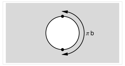
Figure 1: Three-space $M_{3}$ obtained by surgery on three-dimensional Euclidean space $E_{3}$: the interior of a ball with radius $b$ is removed and antipodal points on the boundary of the ball are identified (as indicated by the dots). The “long distance” between antipodal points equals $\pi\,b$ in the original three-space $E_{3}$. (Figure taken from Ref. 1.)

The four-dimensional spacetime manifold has the following topology:

$$M_{4} = \mathbb{R}\times M_{3}\,,$$ (1a)

$$M_{3} = \mathbb{R}P^{3}-p_{\infty}\,,$$ (1b)

where $p_{\infty}$ corresponds to the “point at spatial infinity.” The three-space $M_{3}$ is a noncompact, orientable, nonsimply-connected manifold without boundary. A sketch of the space manifold $M_{3}$ is given in Fig. 1.

A particular covering of $M_{3}$ has three charts of coordinates, labeled by $n=1,2,3$, and details can be found in Ref. 4. These coordinates resemble the standard spherical coordinates and each coordinate chart surrounds one of the three Cartesian coordinate axes but does not intersect the other two axes. The coordinates are denoted

$$(X_{n},\,Y_{n},\,Z_{n})\,,$$ (2)

for $n=1,\,2,\,3$. In each chart, there is one polar-type angular coordinate of finite range, one azimuthal-type angular coordinate of finite range, and one radial-type coordinate with infinite range. Specifically, the coordinates have the following ranges:

$$X_{1} \in(-\infty,\,\infty)\,, Y_{1} \in(0,\,\pi)\,, Z_{1} \in(0,\,\pi)\,,$$ (3a)

$$X_{2} \in(0,\,\pi)\,, Y_{2} \in(-\infty,\,\infty)\,, Z_{2} \in(0,\,\pi)\,,$$ (3b)

$$X_{3} \in(0,\,\pi)\,, Y_{3} \in(0,\,\pi)\,, Z_{3} \in(-\infty,\,\infty)\,.$$ (3c)

The different charts overlap in certain regions, see Ref. 4 for further details. In the present article, we focus on the $n=2$ chart and drop the suffix $2$ on the coordinates,

$$X \in(0,\,\pi)\,, Y \in(-\infty,\,\infty)\,, Z \in(0,\,\pi)\,,$$ (4)

where $Y=0$ indicates the position of the defect surface. Together with the time coordinate $T$, we collectively denote these four spacetime coordinates as $X$. Later, the metric signature will be taken as $(-+++)$.

2.2 Action

The matter fields and their interactions have also been described in Ref. 1, but, as we will make an addition to the theory, we will give some details.

The action reads ($c=\hbar=1$)

$$S = \int_{M_{4}}d^{4}X\,\sqrt{-g}\,\Big{(}\mathcal{L}_{\text{grav}}+\mathcal{L}_{\text{mat}}\Big{)}\,,$$ (5a)

$$\mathcal{L}_{\text{grav}} = \frac{1}{16\pi G_{N}}\>R\,,$$ (5b)

$$\mathcal{L}_{\text{mat}} = \frac{f^{2}}{4}\>\text{tr}\Big{(}\omega_{\mu}\,\omega^{\mu}\Big{)}+\frac{1}{16\,e^{2}}\>\text{tr}\Big{(}\left[\omega_{\mu},\,\omega_{\nu}\right]\left[\omega^{\mu},\,\omega^{\nu}\right]\Big{)}+\frac{1}{2}\,m^{2}\,f^{2}\,\text{tr}\Big{(}\Omega-\mathds{1}_{3}\Big{)}\,,$$ (5c)

$$\omega_{\mu} \equiv \Omega^{-1}\,\partial_{\mu}\,\Omega\,,$$ (5d)

with a Skyrme-type scalar field $\Omega(X)\in SO(3)$. New in (5c) is the mass term proportional to $m^{2}$. Indeed, consider the “pions” $\pi^{a}$ defined by the following expansion:

$$\Omega(X)=\exp\Big{[}S^{a}\,\pi^{a}(X)/f\,\Big{]}\,,$$ (6)

with an implicit sum over $a=1,\,2,\,3$, and $3\times 3$ matrices $S^{a}$ given by

$$S_{1} \equiv \left(\begin{array}[]{ccc}0&0&0\\ 0&0&1\\ \;0&-1&\;0\\ \end{array}\right)\,,\quad S_{2}\equiv\left(\begin{array}[]{ccc}\;0&\;0&-1\\ 0&0&0\\ 1&0&0\\ \end{array}\right)\,,\quad S_{3}\equiv\left(\begin{array}[]{ccc}0&1&0\\ -1&\;0&\;0\\ 0&0&0\\ \end{array}\right)\,.$$ (16)

Incidentally, a useful discussion of the $SO(3)$ Lie group can be found in App. C, pp. 436–438 of Ref. 5. Expanding the $\Omega$ field in (5c) with the Taylor series from (6) and using $\text{tr}(S^{a}S^{b})=-2\,\delta^{ab}$, we have

$$\mathcal{L}_{\text{mat}}=-\frac{1}{2}\,\partial_{\mu}\pi^{a}\partial^{\mu}\pi^{a}-\frac{1}{2}\,m^{2}\,\pi^{a}\pi^{a}+\cdots\,,$$ (17)

which corresponds to three real scalars with equal mass $m$.

The parameters of the theory (5) are Newton’s gravitational coupling constant $G_{N}$ and the energy scale $f>0$ from the kinetic matter term in the action, together with the mass $m$ which we assume to be of order $f$. The first two parameters can be combined in the following dimensionless parameter:

$$\widetilde{\eta} \equiv 8\pi\,G_{N}\,f^{2}\geq 0\,.$$ (18)

The quartic Skyrme term in (5c) has an additional dimensionless real coupling constant,

$$e \in (0,\,\infty)\,.$$ (19)

2.3 Spacetime-defect solution

The self-consistent Ansätze for the metric and the $SO(3)$ matter field have been presented in Ref. 1. For completeness, we give the relevant expressions:

$$ds^{2} = -\big{[}\mu(W)\big{]}^{2}\,dT^{2}+\big{(}1-b^{2}/W\big{)}\,\big{[}\sigma(W)\big{]}^{2}\,(dY)^{2}$$ (20a)

$$+W\Big{[}(dZ)^{2}+\sin^{2}Z\,(dX)^{2}\Big{]}\,,$$

$$\Omega(X) = \cos\big{[}F(W)\big{]}\;\mathds{1}_{3}-\sin\big{[}F(W)\big{]}\;\widehat{x}\cdot\vec{S}+\big{(}1-\cos\big{[}F(W)\big{]}\big{)}\;\widehat{x}\otimes\widehat{x}\,,$$ (20b)

$$W \equiv b^{2}+Y^{2}\,,$$ (20c)

with the matrices $S^{a}$ from (16) and the unit 3-vector $\widehat{x}\equiv\vec{x}/|\vec{x}|$ from the Cartesian coordinates $\vec{x}$ defined in terms of the coordinates $X$, $Y$, and $Z$ (details are in Ref. 4).

The fields of these Ansätze are characterized by the defect length scale $b>0$ (cf. Fig. 1). Henceforth, we will use the Ansatz functions $F(w)$, $\sigma(w)$, and $\mu(w)$ defined in terms of the following dimensionless variable:

$$w\equiv(e\,f)^{2}\;W\in\big{[}(y_{0})^{2},\,\infty\big{)}\,,$$ (21)

where $y_{0}$ is the dimensionless defect scale,

$$y_{0}\equiv e\,f\;b\in\big{(}0,\,\infty\big{)}\,.$$ (22)

The Ansätze (20) reduce the field equations from (5) to the following three ordinary differential equations (ODEs):

$$4\,w\,\sigma^{\prime}(w) = +\sigma(w)\,\left[\left[1-\sigma^{2}(w)\right]+\widetilde{\eta}\,\frac{2}{w}\,\Big{(}A(w)\,\sigma^{2}(w)+C(w)\,\left[w\,F^{\prime}(w)\right]^{2}\Big{)}\right]$$ (23a)

$$+2\,w\,\widetilde{m}^{2}\,\widetilde{\eta}\,\sigma^{3}(w)\,\sin^{2}\frac{F(w)}{2}\,,$$

$$4\,w\,\mu^{\prime}(w) = -\mu(w)\,\left[\left[1-\sigma^{2}(w)\right]+\widetilde{\eta}\,\frac{2}{w}\,\Big{(}A(w)\,\sigma^{2}(w)-C(w)\,\left[w\,F^{\prime}(w)\right]^{2}\Big{)}\right]$$ (23b)

$$-2\,w\,\widetilde{m}^{2}\,\widetilde{\eta}\,\sigma^{2}(w)\,\sin^{2}\frac{F(w)}{2}\,,$$

$$C(w)\,w^{2}\,F^{\prime\prime}(w) = +\sigma^{2}(w)\,\sin F(w)\,\left(\sin^{2}\frac{F(w)}{2}+\frac{w}{2}\right)-\frac{1}{2}\,C(w)\,\sigma^{2}(w)\,w\,F^{\prime}(w)$$ (23c)

$$\times\,\left[1-4\,\widetilde{\eta}\,\frac{1}{w}\,\sin^{2}\frac{F(w)}{2}\,\left(\sin^{2}\frac{F(w)}{2}+w\right)\right]$$

$$-w\,F^{\prime}(w)\,\Big{[}w\,F^{\prime}(w)\,\sin F(w)+w\Big{]}+\frac{\widetilde{m}^{2}}{2}\,w^{2}\,\sigma^{2}(w)\,\sin\frac{F(w)}{2}$$

$$\times\left[\cos\frac{F(w)}{2}+2\,\widetilde{\eta}\,C(w)\,\sin\frac{F(w)}{2}F^{\prime}(w)\right]\,,$$

with a further dimensionless quantity

$$\widetilde{m}^{2}\equiv\frac{1}{e^{2}\,f^{2}}\,m^{2}\,,$$ (24)

and the following auxiliary functions:

$$A(w) \equiv 2\,\sin^{2}\frac{F(w)}{2}\left(\sin^{2}\frac{F(w)}{2}+w\right)\,,$$ (25a)

$$C(w) \equiv 4\,\sin^{2}\frac{F(w)}{2}+w\,.$$ (25b)

These ODEs are to be solved with the following boundary conditions:

$$F(b^{2}) = \pi\,,\quad F(\infty)=0\,,$$ (26a)

$$\sigma(b^{2}) \in (0,\,\infty)\,,$$ (26b)

$$\mu(b^{2}) \in (0,\,\infty)\,,$$ (26c)

where the zero values for $\sigma(b^{2})$ and $\mu(b^{2})$ have been excluded, so that the reduced field equations are well-defined at $Y=0$ (see Sec. 3.3.1 of Ref. 3).

The solutions of the ODEs (23) with boundary conditions (26) behave as follows asymptotically ($w\to\infty$):

$$F(w) \sim \widetilde{k}\,\exp\Big{[}-\widetilde{m}\,\sqrt{w}\,\Big{]}\,\frac{1+\widetilde{m}\,\sqrt{w}}{w}\,,$$ (27a)

$$\sigma(w) \sim \sqrt{1\big{/}\big{(}1-\widetilde{l}/\sqrt{w}\big{)}}\,,$$ (27b)

$$\mu(w) \sim \sqrt{1-\widetilde{l}/\sqrt{w}}\,,$$ (27c)

with constants $\widetilde{k}$ and $\widetilde{l}$. Observe that another contribution $F(w)\propto\exp\big{[}+\widetilde{m}\,\sqrt{w}\,\big{]}$ is eliminated by the boundary condition $F(\infty)=0$.

The reduced expressions for the Ricci curvature scalar $R(w)$, the Kretschmann curvature scalar $K(w)$, and the negative of the 00-component of the Einstein tensor $E^{\mu}_{\;\;\nu}(w)$ $\equiv$ $R^{\mu}_{\;\;\nu}(w)-(1/2)\,R(w)\,\delta^{\mu}_{\;\;\nu}$ have been given in Appendix B of Ref. 1. Here, we present the reduced expression for the 00-component of the energy-momentum tensor $T^{\mu}_{\,\,\nu}(w)$ which corresponds to the negative of the energy density $\rho(w)$,

$$T^{0}_{\,\,0}(w) = -f^{2}\,(e\,f)^{2}\,\frac{2}{w^{2}\,\sigma^{2}(w)}\,$$ (28)

$$\times\Bigg{(}A(w)\,\sigma^{2}(w)+C(w)\,\big{[}w\,F^{\prime}(w)\big{]}^{2}+\widetilde{m}^{2}\,w^{2}\,\sigma^{2}(w)\,\sin^{2}\frac{F(w)}{2}\Bigg{)}\,.$$

The expression in the large brackets on the right-hand side of (28) already appears on the right-hand side of (23a), which results from the 00-component of the Einstein equation.

2.4 Defect solution for $\mathbf{\widetilde{\eta}=0}$

Consider, next, the special theory with $\widetilde{\eta}=0$. Then, the ODE (23a) for $\sigma(w)$ and the ODE (23b) for $\mu(w)$ become independent of the matter function $F(w)$ and can be solved analytically. We obtain the following Schwarzschild-type solutions (cf. Sec. 3 of Ref. 4):

$$\overline{\mu}(w) = \sqrt{1-\widehat{l}/\sqrt{w}}\,,$$ (29a)

$$\overline{\sigma}(w) = \big{[}\overline{\mu}(w)\big{]}^{-1}\,,$$ (29b)

where, for globally regular solutions, the constant $\widehat{l}$ takes values in the following range:

$$\widehat{l}\in(-\infty,\,y_{0})\,.$$ (30)

At $\widetilde{\eta}=0$, the remaining ODE (23c) for $F(w)$ is reduced to the following form:

$$C(w)\,w^{2}\,F^{\prime\prime}(w) = +\overline{\sigma}^{2}(w)\,\sin F(w)\,\Bigg{[}\sin^{2}\frac{F(w)}{2}+\frac{w}{2}\Bigg{]}-\frac{1}{2}\,C(w)\,\overline{\sigma}^{2}(w)\,w\,F^{\prime}(w)$$ (31)

$$-w\,F^{\prime}(w)\,\Bigg{[}w\,F^{\prime}(w)\,\sin F(w)+w\Bigg{]}$$

$$+\frac{\widetilde{m}^{2}}{4}\,w^{2}\,\overline{\sigma}^{2}(w)\,\sin F(w)\,,$$

with $\overline{\sigma}(w)$ given by (29b) and $C(w)$ by (25b). The ODE (31) with boundary conditions (26a) solely depends on the constant $\widehat{l}$, but still cannot be solved analytically.

Physically, the special theory with $\widetilde{\eta}=0$ gives a close approximation to the theory with the matter energy scale $f$ far below the reduced Planck energy scale (the mass $m$ is assumed to be of the same order as $f$),

$$f^{2} \ll \big{(}E_{\text{planck}}\big{)}^{2}\equiv 1/(8\pi G_{N})\approx\big{(}2.44\times 10^{18}\;\text{GeV}\big{)}^{2}\,.$$ (32)

As discussed in App. A of Ref. 2, the theory with a low energy scale (32) and a quartic coupling constant $e\leq 1/\xi$ has anti-gravitating defects if their length scale $b$ is set by the Planck length, $b=\xi\,l_{\text{planck}}$ for a constant $\xi\gtrsim 1$ and with $l_{\text{planck}}\equiv\hbar c/E_{\text{planck}}\approx 8.10\times 10^{-35}\;\text{m}$.

2.5 Gravitational mass of the defect

Finally, introduce the following dimensionless mass-type variable:

$$l(w)\equiv\sqrt{w}\,\left[1-\frac{1}{\sigma^{2}(w)}\right]\,,$$ (33)

which corresponds to a Schwarzschild-type behavior of the square of the metric function,

$$\sigma^{2}(w)=\frac{1}{1-l(w)/\sqrt{w}\,}\,.$$ (34)

The Arnowitt–Deser–Misner (ADM) mass [6] is then obtained by the following limit:

$$M_{\text{ADM}} = \frac{l_{\infty}}{2\,G_{N}\,e\,f}\,,$$ (35a)

$$l_{\infty} \equiv \lim_{w\rightarrow\infty}l(w)\,.$$ (35b)

The task, now, is to find solutions with vanishing ADM mass.

3 Zero-gravitational-mass defect

Numerical results for Skyrmion spacetime defects have been presented in Ref. 2 (further details on the two-dimensional solution space appear in Ref. 3). In fact, Figs. 5 and 6 of Ref. 2 give two numerical solutions with, respectively, negative and positive asymptotic gravitational mass. These two solutions both have boundary conditions (26a), but differ in the boundary condition value of the metric function $\sigma(w)$: $\sigma(b^{2})$ is smaller for the solution of Fig. 5 than for the solution of Fig. 6. For an appropriate intermediate value of $\sigma(b^{2})$, we expect to find a solution with vanishing gravitational mass. The Ansatz functions for this numerical solution are shown in Fig. 3. Practically, these functions have been obtained by integrating inwards from boundary conditions at a large value $w_{\text{max}}$ [specifically, $F(w_{\text{max}})$ and $F^{\prime}(w_{\text{max}})$ from (27a) at $w=w_{\text{max}}$ and $\sigma(w_{\text{max}})$ from (27b) at $w=w_{\text{max}}$ with $\widetilde{l}=0$] and tuning the asymptotic parameter $\widetilde{k}$ to get $F(1)=\pi$.

As mentioned in the caption of Fig. 3, the obtained value for $l_{\infty}$ is very small but not exactly zero. This can, however, be achieved by considering the special theory with $\widetilde{\eta}=0$. Then, it is possible to set $\widehat{l}=0$ in the analytic solutions (29) and also in the corresponding ODE (31) for $F(w)$. The ODE (31) with $\widetilde{m}=0$ and $\overline{\sigma}^{2}(w)=1$ can be solved numerically and the result is shown in Fig. 3.

With a nonzero “pion” mass $m$, the matter fields of the defect solutions have an exponential tail, as shown by (27a) for $\widetilde{m}\neq 0$. Numerical results are given in Figs. 5 and 5. The numerical solutions of Figs. 5 and 5 have an exponentially-vanishing energy density of the matter fields, together with a vanishing ADM mass. In fact, the ADM mass of Fig. 5 is exactly zero.

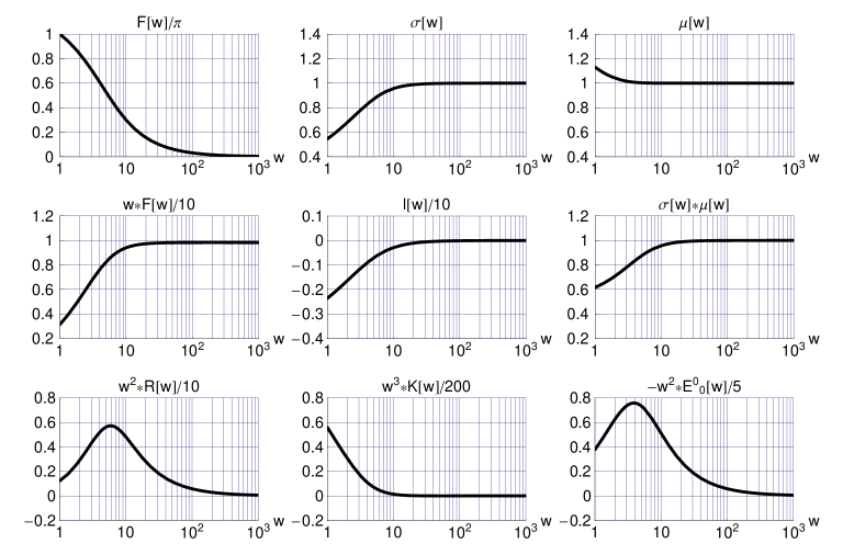
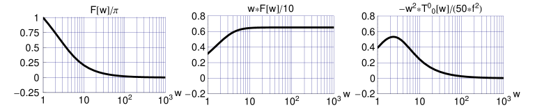
Figure 2: (Top row) Ansatz functions $F(w)$, $\sigma(w)$, and $\mu(w)$ of the numerical solution of the ODEs (23) with $\widetilde{m}=0$. The parameters are $\widetilde{\eta}\equiv 8\pi\,G_{N}\,f^{2}=1/10$ and $y_{0}\equiv efb=1$. The boundary conditions at the defect surface $w=y_{0}^{2}=1$ are: $F/\pi=1.00000$, $F^{\prime}=-0.569030$, $\sigma=0.545346$, and $\mu=1.13031$. (Middle row) Derived functions $w\,F(w)$, $l(w)\equiv\sqrt{w}\,\left[1-1/\sigma^{2}(w)\right]$, and $\sigma(w)\,\mu(w)$. For the functions shown, the value of $|l(w)|$ is less than $10^{-6}$ over the interval $w\in[10^{3},\,10^{7}]$. (Bottom row) Dimensionless Ricci curvature scalar $R(w)$, dimensionless Kretschmann curvature scalar $K(w)$, and negative of the 00-component of the dimensionless Einstein tensor $E^{\mu}_{\;\;\nu}(w)$ $\equiv$ $R^{\mu}_{\;\;\nu}(w)-(1/2)\,R(w)\,\delta^{\mu}_{\;\;\nu}$. See Appendix B of Ref. 1 for the explicit expressions of $R(w)$, $K(w)$, and $E^{0}_{\;\;0}(w)$.

Figure 3: Same as Fig. 3, but with $\widetilde{\eta}=0$. The ODEs for the metric functions $\sigma(w)$ and $\mu(w)$ can then be solved analytically and take the Schwarzschild form (29). Here, the Schwarzschild parameter $\widehat{l}$ is taken to vanish exactly, which implies that the corresponding ADM mass (35) also vanishes exactly [the spacetime manifold is flat with, in particular, $R(w)=K(w)=E^{0}_{\;\;0}(w)=0$]. The corresponding ODE (31) for $F(w)$, with $\widetilde{m}=0$ and $\overline{\sigma}^{2}(w)=1$, has the following boundary conditions at the defect surface $w=y_{0}^{2}=1$: $F=\pi$ and $F^{\prime}=-1077934703/10^{9}$. The right panel shows the energy density of the matter fields, with the energy-momentum-tensor component $T^{0}_{\,\,0}(w)=-\rho(w)$ given by (28).

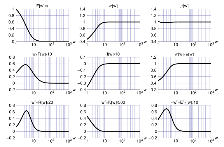
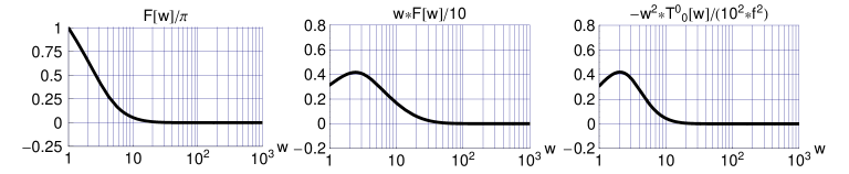
Figure 4: Same as Fig. 3, but with $\widetilde{m}=1$. The boundary conditions at the defect surface $w=y_{0}^{2}=1$ are: $F/\pi=1.00000$, $F^{\prime}=-0.752388$, $\sigma=0.466343$, and $\mu=1.02282$. For the functions shown, the value of $|l(10^{3})|$ is less than $10^{-11}$.

Figure 5: Same as Fig. 3, but with $\widetilde{m}=1$. The boundary conditions at the defect surface $w=y_{0}^{2}=1$ are: $F/\pi=1.00000$ and $F^{\prime}=-1.43972$. As in Fig. 3, the ADM mass vanishes exactly and spacetime is flat.

The solution of Fig. 5 is a prime example of what we propose to call a “stealth defect.” Outside this stealth defect, the matter fields $\pi^{a}$ from (6) rapidly vanish and the spacetime is flat (Minkowskian away from the defect surface). Light rays follows straight paths and pass through the defect: for radial paths crossing the defect surface, the rays go straight through [4], but, for non-radial paths crossing the defect surface, the rays are parallel lines shifted by the identification of antipodal points on the defect surface.

4 Discussion

In this article, we have discussed a particular type of Skyrmion spacetime-defect solution [1], which has a vanishing asymptotic gravitational mass. As to the origin of this zero mass, we observe that there is a positive mass contribution from the matter fields but a negative “effective mass” from the gravitational fields at the defect surface $Y=0$. As explained in our previous article [2] and recalled in the third paragraph of Sec. 1, this negative “effective mass” at the defect surface is needed in order to have a globally regular solution if the defect scale $b$ is small enough.

For the solution of Fig. 5 in particular, the matter energy density is exponentially vanishing towards infinity (as long as $m^{2}\neq 0$) and the monopole term of the gravitational field is absent ($M_{\text{ADM}}=0$ exactly). With a spherically symmetric defect surface and with a spherically symmetric matter distribution, we also expect no higher-order terms of the gravitational field (quadrupole, octupole, etc.), but this expectation needs to be confirmed.

Now, assume that all matter fields have some form of non-gravitational interaction with each other. If so, there will, in principle, be some interaction between the “pions” of the theory considered in (5) and the elementary particles of the standard model. Then, consider what happens with a head-on collision of a stealth defect and an observer made of standard-model particles (mostly up and down quarks, gluons, and electrons). In close approximation, the observer will have no idea of what is going to happen, until he/she is within a distance of order $h/(mc)$ from the defect, where $m$ is the “pion” mass scale from the matter action (5c). What happens during the collision itself and afterwards depends on the details of the setup, for example, the size of the observer compared to the defect scale $b$. The only point we are sure of is that, assuming the existence of this particular type of spacetime-defect solution without long-range fields, an observer has no advance warning if he/she approaches such a stealth-type defect solution (displacement effects of background stars are negligible, at least initially).

5 Outlook

The topic of the present article, a stealth-type soliton solution, is related to the larger physics issue of invisibility. The prime example is an invisibility cloak which can be wrapped around a massive object in order to, more or less, hide the object from an outside observer (see, e.g., Refs. 7, 8, 9, 10 and references therein). Still, the wrapped object has a gravitational mass and is, as such, detectible by its gravitational force on a distant test particle.

In a way, these two types of systems, cloaked object and stealth defect, are orthogonal to each other. The cloaked object, on the one hand, is more or less invisible for light but can still be detected by its asymptotic gravitational mass, $M_{\text{ADM}}>0$. The stealth defect, on the other hand, cannot be detected by its asymptotic gravitational mass, $M_{\text{ADM}}=0$, but is not really invisible for light (assuming that the matter fields of the defect have interactions with photons).

For the stealth defect, the role of the “gravitational invisibility cloak” is played by the defect surface and its nontrivial gravitational fields (as discussed in the second and third paragraphs of Sec. 1): these gravitational fields make the matter fields just outside the defect surface gravitationally invisible at infinity. For the stealth-defect system, this “gravitational invisibility cloak” is buried inside the matter, instead of wrapping around the energy density distribution of the matter.

As a final speculative comment, we could try to hide a massive object by placing an appropriate spacetime defect next to it and wrapping the whole in an invisibility cloak. The defect must have the appropriate negative gravitational mass, so that the total gravitational mass of object+defect+cloak is zero. In addition, the cloak must be strong enough, because the material object receives a repulsive gravitational force from the defect.

Expanding on the last comment, we may consider the present article as a small step towards the “applied physics of the future,” which deals with designing and modelling spacetime in addition to designing and modelling ponderable matter. In this respect, we should mention that the crucial open question is the origin and role of nontrivial spacetime topology (see, in particular, Chap. 6 of Ref. 11). Specialized to our Skyrmion spacetime-defect solution, the questions are what sets the constant defect scale $b$ and can this defect scale become a dynamic variable? These and other theoretical questions need to be addressed before we can really start thinking about the “applied physics of the future.”

References

- [1] F.R. Klinkhamer, “Skyrmion spacetime defect,” Phys. Rev. D 90, 024007 (2014), arXiv:1402.7048.
- [2] F.R. Klinkhamer and J.M. Queiruga, “Antigravity from a spacetime defect,” Phys. Rev. D 97, 124047 (2018), arXiv:1803.09736.
-
[3]
M. Guenther,
“Skyrmion spacetime defect, degenerate metric,
and negative gravitational mass,”
Master Thesis, KIT, September 2017;
available from
https://www.itp.kit.edu/en/publications/diploma - [4] F.R. Klinkhamer, “A new type of nonsingular black-hole solution in general relativity,” Mod. Phys. Lett. A 29, 1430018 (2014), arXiv:1309.7011.
- [5] B. De Wit and J. Smith, Field Theory in Particle Physics, Volume 1 (North-Holland Physics Publishing, Amsterdam, The Netherlands, 1986).
- [6] R. Arnowitt, S. Deser, and C.W. Misner, “Dynamical structure and definition of energy in general relativity,” Phys. Rev. 116, 1322 (1959).
- [7] J. B. Pendry, D. Schurig, and D. R. Smith, “Controlling electromagnetic fields,” Science 312, 1780 (2006).
- [8] U. Leonhardt, “Optical conformal mapping,” Science 312, 1777 (2006), arXiv: physics/0602092v1.
- [9] J.C. Halimeh, R.T. Thompson, and M. Wegener, “Invisibility cloaks in relativistic motion,” Phys. Rev. A 93, 013850 (2016), arXiv:1510.06144.
- [10] R. Schittny, A. Niemeyer, F. Mayer, A. Naber, M. Kadic, and M. Wegener, “Invisibility cloaking in light-scattering media,” Laser Photonics Rev. 10, 382 (2016).
- [11] M. Visser, Lorentzian Wormholes: From Einstein to Hawking (Springer-Verlag, New York, USA, 1995).