Fast magnetic field evolution in neutron stars: the key role of magnetically induced fluid motions in the core

Abstract

In [Gusakov et al. PRD, 96, 103012, (2017)], we proposed a self-consistent method to study the quasistationary evolution of the magnetic field in neutron-star cores. Here we apply it to calculate the instantaneous particle velocities and other parameters of interest, which are fixed by specifying the magnetic field configuration. Interestingly, we found that the magnetic field can lead to generation of a macroscopic fluid motion with the velocity, significantly exceeding the diffusion particle velocities. This result calls into question the standard view on the magnetic field evolution in neutron stars and suggests a new, shorter timescale for such evolution.

I Introduction

One of the most interesting problems in the neutron star (NS) physics concerns the evolutionary relationships between various classes of NSs with often very different surface magnetic fields ranging from, e.g., $10^{8}-10^{10}$ G in millisecond pulsars to $\sim 10^{12}$ G in ordinary radio pulsars and up to $\sim 10^{15}$ G in magnetars. What makes these fields so different? The complete answer is still unknown in spite of a lot of effort devoted to this problem in the past. Obviously, the magnetic field at the stellar surface should be related somehow to that in NS interiors. So far, most of the research has been focused on the magnetic field evolution in the crust (e.g., Refs. Jones (1988); Shalybkov and Urpin (1997); Rheinhardt and Geppert (2002); Hollerbach and Rüdiger (2004); Gourgouliatos et al. (2013); Viganò et al. (2013); Gourgouliatos and Cumming (2014a); Gourgouliatos et al. (2016)). The evolution in the core has been studied less intensively (see, e.g., Refs. Elfritz et al. (2016); Bransgrove et al. (2018); Passamonti et al. (2017); Castillo et al. (2017)). In part, this is because such an analysis is substantially more complex, while the physics involved is not well understood, and in part because of the widespread opinion (but see Refs. Jones (2006); Bransgrove et al. (2018)) that the evolution in the crust proceeds on a shorter timescale than in the core.

This work continues our study of the magnetic field evolution in NS cores. Recently, we have solved the following problem Gusakov et al. (2017). Assume that there is an NS with some (specified) magnetic field $\boldsymbol{B}(t_{0})$ at the initial moment of time $t=t_{0}$. What will be the magnetic field in the next moment $t=t_{0}+\delta t$? The answer to this question is provided by the Faraday’s law, $\boldsymbol{B}(t_{0}+\delta t)=\boldsymbol{B}(t_{0})-c\,\delta t\operatorname{curl}{\boldsymbol{E}}(t_{0})$, so the problem reduces to finding the self-consistent electric field $\boldsymbol{E}$ at $t=t_{0}$. The latter field depends, in turn, on perturbations of particle chemical potentials and various particle velocities induced by the magnetic field. In Ref. Gusakov et al. (2017) we proposed a method to self-consistently calculate all these quantities. We also found that the previous works, exploring the same problem (see, e.g., Refs. Goldreich and Reisenegger (1992); Thompson and Duncan (1996); Hoyos et al. (2008); Reisenegger (2009); Hoyos et al. (2010); Glampedakis et al. (2011a); Beloborodov and Li (2016); Passamonti et al. (2017); Castillo et al. (2017)), have made some unjustified simplifications, that can qualitatively change the results.

Here our aim is to further develop the method of Ref. Gusakov et al. (2017) and to demonstrate its ability to calculate all the ingredients necessary to follow the evolution of $\boldsymbol{B}$ in time. For this purpose, we adopt a model of an NS core consisting of nonsuperfluid neutrons ($n$), nonsuperconducting protons ($p$), and electrons ($e$). Although very simplistic, this model may be adequate in describing hot magnetars with very high magnetic field, resulting in a partly (or fully) suppressed nucleon superfluidity/superconductivity in their cores Sinha and Sedrakian (2015); Sedrakian et al. (2017). The main advantage of the model is that it allows for relatively simple and transparent calculations, the disadvantage is that it ignores the effects of baryon superfluidity/superconductivity, and thus is not directly applicable to cold NSs with relatively low magnetic field (e.g., radio- and millisecond pulsars); evolution of the magnetic field in such stars will be considered by us elsewhere.

The main result in the paper consists in demonstrating that the relative particle velocities (generated by the magnetic field) can generally be much smaller than the velocity of the fluid as a whole. This result is important since it introduces a new small timescale into the problem of the magnetic field evolution in NSs. It also contradicts the general belief that NS matter is motionless to a good approximation in the presence of the magnetic field (e.g., Goldreich and Reisenegger (1992); Thompson and Duncan (1996); Beloborodov and Li (2016); Passamonti et al. (2017); Castillo et al. (2017)).

The paper is organized as follows. Sec. II discusses magnetohydrodynamic equations and various approximations that were made to solve them. In Sec. III we propose a detailed analytic solution to these equations. Sec. IV contains description of the adopted magnetic field models and our numerical results. Finally, discussion and conclusions are presented in Sec. V.

II General equations and quasistationary approximation

In this section we formulate and briefly discuss the magnetohydrodynamic (MHD) equations for nonsuperfluid and nonsuperconducting matter of NSs composed of various particle species. The equation of state (EOS) is assumed to be relativistic, but the effects of general relativity will be disregarded for simplicity. We also neglect (weak) thermal forces in the equations of motion for each particle species, as well as the effects of temperature on the EOS. With these simplifications, the system of MHD equations can be written as (e.g., Iakovlev and Shalybkov (1991); Goldreich and Reisenegger (1992); Gusakov et al. (2017))

$$\frac{\partial n_{a}}{\partial t}+\operatorname{div}\left(n_{a}\boldsymbol{u}_{a}\right)=\Delta\Gamma_{a},$$ (1a)

$$n_{a}\left[\frac{\partial}{\partial t}+\left(\boldsymbol{u}_{a}\boldsymbol{\nabla}\right)\right]\left(\frac{\mu_{a}}{c^{2}}\boldsymbol{u}_{a}\right)=-n_{a}\boldsymbol{\nabla}\mu_{a}+e_{a}n_{a}\left(\boldsymbol{E}+\frac{\boldsymbol{u}_{a}}{c}\times\boldsymbol{B}\right)-\frac{\mu_{a}n_{a}}{c^{2}}\boldsymbol{\nabla}\phi-\sum_{b\neq a}J_{ab}\left(\boldsymbol{u}_{a}-\boldsymbol{u}_{b}\right),$$ (1b)

$$\Delta\phi=\frac{4\pi G}{c^{2}}(P+\varepsilon),$$ (1c)

$$\sum_{a}e_{a}n_{a}=0,$$ (1d)

$$\frac{c}{4\pi}\operatorname{curl}\boldsymbol{B}=\sum_{a}e_{a}n_{a}\boldsymbol{u}_{a}=\boldsymbol{j},$$ (1e)

$$\frac{\partial\boldsymbol{B}}{\partial t}=-c\operatorname{curl}\boldsymbol{E}.$$ (1f)

Eqs. (1a) and (1b) should be satisfied for each particle species “$a$” separately. Here $e_{a}$, $n_{a}$, $\mu_{a}$, and $\boldsymbol{u}_{a}$ are, respectively, the electric charge, number density, chemical potential, and velocity for particles “$a$”; $\Delta\Gamma_{a}$ is the reaction rate for species “$a$” due to nonequilibrium processes of particle mutual transformations; $J_{ab}=J_{ba}$ is the coefficient in the expression for the friction force, $-J_{ab}(\boldsymbol{u}_{a}-\boldsymbol{u}_{b})$, describing friction between species $a$ and $b$; it is related to the effective relaxation time, $\tau_{ab}$, by the formula Iakovlev and Shalybkov (1991): $J_{ab}=n_{a}\mu_{a}/(\tau_{ab}c^{2})$. Further, $\phi$ is the Newtonian gravitational potential, $G$ and $c$ are, respectively, the gravitational constant and the speed of light; $P$ and $\varepsilon=\rho c^{2}$ are the total pressure and energy density (proportional to the total density of matter $\rho$); $\boldsymbol{j}$, $\boldsymbol{E}$, and $\boldsymbol{B}$ are the electric current density, electric, and magnetic fields, respectively.

The thermodynamic parameters appearing in Eqs. (1) are not all independent and are related by the following formulas, valid in strongly degenerate matter,

$$P+\varepsilon =\sum_{a}n_{a}\mu_{a},$$ (2a)

$$\mathrm{d}P =\sum_{a}n_{a}\mathrm{d}\mu_{a}.$$ (2b)

In what follows we consider only small perturbations of the system (1) assuming that unperturbed state describes a nonmagnetized NS with the core composed of neutrons ($n$), protons ($p$), and electrons ($e$) in full hydrostatic and thermodynamic equilibrium. Correspondingly, in the unperturbed star $\boldsymbol{u}_{a}=0$ and $\Delta\Gamma_{a}=0$ for $a=n$, $p$, $e$, while other parameters (e.g., the number densities $n_{a}$) are the only functions of the radial coordinate $r$ (here and hereafter we make use of the spherical coordinates $r$, $\theta$, and $\varphi$).

Now let us slightly perturb the star by creating some small currents that will generate the magnetic field in the system. Following the standard approach of Ref. Goldreich and Reisenegger (1992) (see also, e.g., Refs. Passamonti et al. (2017); Castillo et al. (2017); Gusakov et al. (2017); Glampedakis et al. (2011a); Beloborodov and Li (2016)) we assume that the perturbed star is in the quasistationary equilibrium and is stable with respect to spontaneous reconfiguration of the magnetic field. This allows us to neglect time derivatives in the Euler and the continuity equations, as discussed in detail below. The generated magnetic field causes small deviations $\delta n_{a}$, $\delta\mu_{a}$, $\delta\boldsymbol{E}$, and $\delta\phi$ of the quantities $n_{a}$, $\mu_{a}$, $\boldsymbol{E}$, and $\phi$ from their unperturbed values $n_{a0}$, $\mu_{a0}$, $\boldsymbol{E}_{0}$, and $\phi_{0}$. This launches two dissipation mechanisms: nonequilibrium reactions [see the reaction rates $\Delta\Gamma_{a}$ in Eq. (1a)] and diffusion with small but non-zero particle velocities $\boldsymbol{u}_{a}$ [see the corresponding friction forces, $-J_{ab}(\boldsymbol{u}_{a}-\boldsymbol{u}_{b})$, in Eq. (1b)]. For $npe$-cores of NSs the only nonequilibrium reactions that generate $\Delta\Gamma_{a}$ are the direct and modified Urca processes. The corresponding rates $\Delta\Gamma_{n}=-\Delta\Gamma_{e}=-\Delta\Gamma_{p}\equiv\Delta\Gamma$ were calculated in Ref. Reisenegger (1995a), where it was shown that $\Delta\Gamma$ can be presented as the function of the chemical potential imbalance, $\Delta\mu\equiv\mu_{e}+\mu_{p}-\mu_{n}=\delta\mu_{e}+\delta\mu_{p}-\delta\mu_{n}$. The expressions for these rates, as well as for the coefficients $J_{ab}$ are presented in Ref. Gusakov et al. (2017); we use the same expressions in all our calculations and refer the interested reader to that reference for more details. However, for subsequent presentation it is important to note that the electron-neutron friction coefficient $J_{en}$ is much smaller than other coefficients, $J_{np},\,J_{ep}\gg J_{en}$, and therefore can be ignored. In what follows $J_{np}$, $J_{ep}$, and $\Delta\Gamma$ are treated as given explicit functions of unperturbed number densities $n_{a}$ and temperature $T$.

Now our aim is to write down Eqs. (1) for a perturbed star. Let us, for example, consider equation of motion (1b) for a particle species $a$

$$n_{a}\left[\frac{\partial}{\partial t}+\left(\boldsymbol{u}_{a}\boldsymbol{\nabla}\right)\right]\left(\frac{\mu_{a}}{c^{2}}\boldsymbol{u}_{a}\right)=\delta n_{a}\left(-\boldsymbol{\nabla}\mu_{a}+e_{a}\boldsymbol{E}-\frac{\mu_{a}}{c^{2}}\boldsymbol{\nabla}\phi\right)-\frac{n_{a}}{c^{2}}\left(\delta\mu_{a}\boldsymbol{\nabla}\phi+\mu_{a}\boldsymbol{\nabla}\delta\phi\right)-\\ -n_{a}\boldsymbol{\nabla}\delta\mu_{a}+e_{a}n_{a}\left(\delta\boldsymbol{E}+\frac{\boldsymbol{u}_{a}}{c}\times\boldsymbol{B}\right)-\sum_{b\neq a}J_{ab}(\boldsymbol{u}_{a}-\boldsymbol{u}_{b}).$$ (3)

Here and below to simplify notation, $n_{a}$, $\mu_{a}$, $\boldsymbol{E}$, and $\phi$ stand for the unperturbed quantities. Note that even in the full equilibrium $\boldsymbol{E}\neq 0$, since a self-consistent electric field is generated in order to preserve the quasineutrality condition, $n_{e}=n_{p}$ (see Eq. 1d). The first term on the right-hand side of this equation vanishes because $-\boldsymbol{\nabla}\mu_{a}+e_{a}\boldsymbol{E}-\mu_{a}\boldsymbol{\nabla}\phi/c^{2}=0$ for a star in hydrostatic equilibrium. Eq. (3) (and other equations in the system 1) can be further simplified provided that we make some reasonable approximations, which were discussed in detail in Refs. Goldreich and Reisenegger (1992); Passamonti et al. (2017); Gusakov et al. (2017).

(i) We neglect perturbations of gravitational potential $\delta\phi$ (Cowling approximation Cowling (1941)) and, moreover, the term $n_{a}\delta\mu_{a}\boldsymbol{\nabla}\phi/c^{2}$, since it have to be much smaller than $n_{a}\boldsymbol{\nabla}\delta\mu_{a}$ for a Newtonian star for which Eq. (3) is written. Thus only the last three terms survive in the right-hand side of Eq. (3).

(ii) We use a quasistationary approximation. In our problem the magnetic field $\boldsymbol{B}$ is the only perturbing factor that drives the system out of the equilibrium. Let $\tau_{B}$ and $L_{B}$ be the typical timescale and lengthscale of $\boldsymbol{B}$ evolution. Then one can estimate $\partial/\partial t\sim 1/\tau_{B}$, $\nabla\sim\operatorname{div}\sim\operatorname{curl}\sim 1/L_{B}$, and $u_{a}\sim L_{B}/\tau_{B}$ in Eqs. (1) and (3). Correspondingly, the left-hand side of Eq. (3) can be estimated as

$$n_{a}\left[\frac{\partial}{\partial t}+(u_{a}\nabla)\right]\left(\frac{\mu_{a}}{c^{2}}u_{a}\right)\sim n_{a}\frac{\mu_{a}u_{a}}{c^{2}\tau_{B}}\sim n_{a}\frac{\mu_{a}}{L_{B}}\frac{L_{B}}{c\tau_{B}}\frac{u_{a}}{c}\sim n_{a}\frac{\mu_{a}}{L_{B}}\frac{u_{a}^{2}}{c^{2}}.$$ (4)

In turn, the terms in the right-hand side of Eq. (3) are of the order of $n_{a}\mu_{a}B^{2}/(8\pi PL_{B})$ Gusakov et al. (2017), so that the left-hand side terms can be safely neglected provided that $(u_{a}^{2}/c^{2})(8\pi P)/B^{2}\ll 1$ which is always the case for the typical NS conditions. Similar estimate can be made for the continuity equation (1a) where the time derivatives can also be omitted provided that $B^{2}/(8\pi P)\ll 1$ Goldreich and Reisenegger (1992); Gusakov et al. (2017).

(iii) The system is assumed to be axisymmetric, i.e., $\boldsymbol{B}$ and all the perturbations depend exclusively on $r$ and $\theta$.

Using the above approximations the system of equations, describing $\boldsymbol{B}$-evolution, takes the form (see also Ref. Gusakov et al. (2017))

$$\operatorname{div}(n_{n}\boldsymbol{u}_{n})=-\operatorname{div}(n_{e}\boldsymbol{u}_{p})=-\operatorname{div}(n_{e}\boldsymbol{u}_{e})=\Delta\Gamma,$$ (5a)

$$n_{n}\boldsymbol{\nabla}\delta\mu_{n}+J_{np}(\boldsymbol{u}_{n}-\boldsymbol{u}_{p})=0,$$ (5b)

$$n_{e}\boldsymbol{\nabla}\delta\mu_{e}+J_{ep}(\boldsymbol{u}_{e}-\boldsymbol{u}_{p})=-en_{e}\left(\delta\boldsymbol{E}+\frac{\boldsymbol{u}_{e}}{c}\times\boldsymbol{B}\right),$$ (5c)

$$n_{n}\boldsymbol{\nabla}\delta\mu_{n}+n_{e}\boldsymbol{\nabla}(\delta\mu_{p}+\delta\mu_{e})=\boldsymbol{f}_{A},$$ (5d)

$$\boldsymbol{j}=en_{e}(\boldsymbol{u}_{p}-\boldsymbol{u}_{e}),$$ (5e)

$$\frac{\partial\boldsymbol{B}}{\partial t}=-c\operatorname{curl}\delta\boldsymbol{E}.$$ (5f)

where $e=e_{p}$ is the elementary charge and $\boldsymbol{f}_{A}$ is the Ampere force,

$$\boldsymbol{f}_{A}=\frac{1}{c}\,[\boldsymbol{j}\times\boldsymbol{B}].$$ (6)

In the Euler Eqs. (5b)–(5d) the equation for protons is replaced with the total force balance Eq. (5d), which is a sum of Euler equations over all particle species. Note that Eq. (5d) ensures that the system is in hydrostatic equilibrium during its (quasistationary) evolution. The quasineutrality condition (1d) is accounted for by substituting $n_{p}$ for $n_{e}$ in Eqs. (5); the unperturbed electric field does not appear in Eq. (5f) since it is purely potential.

Now our aim is to find the particle velocities $\boldsymbol{u}_{a}$ from Eqs. (5), induced by the presence of an axisymmetric magnetic field (which is assumed to be specified). As a by-product of this calculation, we will also find $\delta\boldsymbol{E}$ and, consequently, $\partial\boldsymbol{B}/\partial t$ (see Eq. 5f). This will open an exciting possibility to follow the quasistationary evolution of the magnetic field by simply iterating Eq. (5f) in time.

III Solution to Eqs. (5)

First, let us define the baryon velocity $\boldsymbol{U}_{b}$ and the diffusion velocities $\boldsymbol{w}_{a}$ according to the equations

$$\boldsymbol{U}_{b}\equiv\frac{n_{n}}{n_{b}}\boldsymbol{u}_{n}+\frac{n_{p}}{n_{b}}\boldsymbol{u}_{p}=\frac{n_{n}}{n_{b}}\boldsymbol{u}_{n}+\frac{n_{e}}{n_{b}}\boldsymbol{u}_{p},\qquad\boldsymbol{w}_{a}\equiv\boldsymbol{u}_{a}-\boldsymbol{U}_{b},$$ (7)

where $n_{b}\equiv n_{n}+n_{p}=n_{n}+n_{e}$ is the baryon number density. Second, let us introduce the electric field ${\boldsymbol{E}}_{\rm com}$ in the frame, locally comoving with the baryons, that is

$$\delta\boldsymbol{E}_{\text{com}}=\delta\boldsymbol{E}+\frac{\boldsymbol{U}_{b}}{c}\times\boldsymbol{B}.$$ (8)

We assume that the (axisymmetric) instantaneous magnetic field $\boldsymbol{B}$ is specified, i.e., we know the function ${\boldsymbol{B}}(r,\,\theta)$ at some moment of time (but the time dependence of ${\boldsymbol{B}}$ is unknown!). In view of Eqs. (1e) and (6) this means that the vectors $\boldsymbol{j}$ and $\boldsymbol{f}_{A}$ are also specified. In what follows it will be convenient to rewrite the Faraday’s law in terms of the quantities $\delta\boldsymbol{E}_{\text{com}}$ and $\boldsymbol{U}_{b}$. Plugging Eq. (8) into (5f), we get

$$\frac{\partial\boldsymbol{B}}{\partial t}=-c\operatorname{curl}\delta\boldsymbol{E}_{\text{com}}+\operatorname{curl}\left(\boldsymbol{U}_{b}\times\boldsymbol{B}\right).$$ (9)

Thus, in order to trace the evolution of the magnetic field, one has to determine the comoving electric field and the baryon velocity. Note that in Ref. Gusakov et al. (2017) we used the net flow velocity $\boldsymbol{U}=\sum_{a}\mu_{a}n_{a}\boldsymbol{u}_{a}/(P+\varepsilon)$ instead of $\boldsymbol{U}_{b}$. This approach is equivalent to that employed here since $\boldsymbol{U}_{b}=\boldsymbol{U}+\boldsymbol{j}\mu_{e}/[e(P+\varepsilon)]$.

III.1 Finding $\boldsymbol{w}_{a}$ and $\delta\boldsymbol{E}_{\rm com}$

Let us assume for a while that the quantities $\delta\mu_{a}$ are known. Then we can easily find the vectors $\boldsymbol{w}_{a}$ (which are the velocities of particle species $a$ in the frame comoving with baryons, $\boldsymbol{U}_{b}=0$). Using Eqs. (5b), (5e), and (7), one has

$$J_{np}\left(\boldsymbol{w}_{n}-\boldsymbol{w}_{p}\right) =-n_{n}\boldsymbol{\nabla}\delta\mu_{n},$$ (10a)

$$en_{e}\left(\boldsymbol{w}_{p}-\boldsymbol{w}_{e}\right) =\boldsymbol{j},$$ (10b)

$$n_{n}\boldsymbol{w}_{n}+n_{e}\boldsymbol{w}_{p} =0.$$ (10c)

The solution to this system is

$$\boldsymbol{w}_{n} =-\frac{n_{e}n_{n}}{n_{b}J_{np}}\boldsymbol{\nabla}\delta\mu_{n},$$ (11a)

$$\boldsymbol{w}_{p} =\frac{n_{n}^{2}}{n_{b}J_{np}}\boldsymbol{\nabla}\delta\mu_{n},$$ (11b)

$$\boldsymbol{w}_{e} =\frac{n_{n}^{2}}{n_{b}J_{np}}\boldsymbol{\nabla}\delta\mu_{n}-\frac{\boldsymbol{j}}{en_{e}}.$$ (11c)

Eqs. (5c), (8), and (11c) give

$$\delta\boldsymbol{E}_{\text{com}}=-\frac{\boldsymbol{\nabla}\delta\mu_{e}}{e}+\frac{J_{ep}}{e^{2}n_{e}^{2}}\boldsymbol{j}-\frac{n_{n}^{2}}{cn_{b}J_{np}}\boldsymbol{\nabla}\delta\mu_{n}\times\boldsymbol{B}+\frac{\boldsymbol{f}_{A}}{en_{e}}.$$ (12)

Actually, in order to follow the magnetic field evolution, we are interested in the quantity ${\rm curl}\,\delta\boldsymbol{E}_{\text{com}}$ rather than in $\delta\boldsymbol{E}_{\text{com}}$ (see Eq. 9). This means, in particular, that there is no need in calculation of the term $\boldsymbol{\nabla}\delta\mu_{e}/e$ in Eq. (12).

Note that Eqs. (11) and (12) can also be obtained using a diffusion tensor from Ref. Iakovlev and Shalybkov (1991), but this way of derivation is more sophisticated. It leads to the generalized form of the Ohm’s law Shalybkov and Urpin (1995), which is equivalent to Eqs. (11) and (12).

III.2 Finding the poloidal component of the baryon velocity $\boldsymbol{U}_{b}$

First, let us note that, according to Eqs. (5a) and (7), the baryon velocity is purely solenoidal,

$$\operatorname{div}\left(n_{b}\boldsymbol{U}_{b}\right)=0.$$ (13)

Recalling that the system is axisymmetric, the expression for the poloidal component of the baryon velocity can be presented as

$$n_{b}\boldsymbol{U}_{b}^{(p)}=\operatorname{curl}\left[\Upsilon(r,\theta)\boldsymbol{\nabla}\varphi\right]=\boldsymbol{\nabla}\Upsilon\times\boldsymbol{\nabla}\varphi,$$ (14)

where $\boldsymbol{\nabla}\varphi=\boldsymbol{e}_{\varphi}/(r\sin\theta)$; the superscript “${(p)}$” denotes the poloidal component of a vector field; and $\Upsilon$ is an arbitrary function of $r$ and $\theta$. This decomposition is widely used for poloidal magnetic fields (see, e.g., Ref. Goedbloed et al. (2010) and Sec. III.5). Then, plugging Eqs. (7) and (14) into Eq. (5a) for protons, we have

$$\operatorname{div}\left(n_{e}\boldsymbol{u}_{p}\right)=\operatorname{div}\left(\frac{n_{e}}{n_{b}}\boldsymbol{\nabla}\Upsilon\times\boldsymbol{\nabla}\varphi\right)+\operatorname{div}\left(n_{e}\boldsymbol{w}_{p}\right)=\boldsymbol{\nabla}\left(\frac{n_{e}}{n_{b}}\right)\cdot\left(\boldsymbol{\nabla}\Upsilon\times\boldsymbol{\nabla}\varphi\right)+\operatorname{div}\left(n_{e}\boldsymbol{w}_{p}\right)=-\Delta\Gamma.$$ (15)

Employing Eq. (11b), we arrive at

$$\left[\boldsymbol{\nabla}\varphi\times\boldsymbol{\nabla}\left(\frac{n_{e}}{n_{b}}\right)\right]\cdot\boldsymbol{\nabla}\Upsilon=-\operatorname{div}\left(\frac{n_{e}n_{n}^{2}}{n_{b}J_{np}}\boldsymbol{\nabla}\delta\mu_{n}\right)-\Delta\Gamma.$$ (16)

Since $\partial n_{a}/\partial\theta=\partial n_{a}/\partial\varphi=0$, this equation takes the form

$$\frac{\partial\Upsilon}{\partial\theta}=n_{b}r^{2}V(r,\theta)\sin\theta,$$ (17)

where

$$V=\frac{n_{b}}{n_{b}^{\prime}n_{e}-n_{e}^{\prime}n_{b}}\left[\operatorname{div}\left(\frac{n_{e}n_{n}^{2}}{n_{b}J_{np}}\boldsymbol{\nabla}\delta\mu_{n}\right)+\Delta\Gamma\right],$$ (18)

and a prime sign $(^{\prime})$ stands for $\mathrm{d}/\mathrm{d}r$. The solution to Eq. (17) is

$$\Upsilon(r,\theta)=n_{b}r^{2}\int_{0}^{\theta}V(r,\tilde{\theta})\sin\tilde{\theta}\mathrm{d}\tilde{\theta}+\xi(r),$$ (19)

where $\xi(r)$ is an arbitrary function. Plugging this solution into Eq. (14), we find an expression for the poloidal component of the baryon velocity, which contains the term $\xi^{\prime}(r)/(r\sin\theta)$. This velocity must be finite at the symmetry axis, $\theta=0$, which leads to the condition $\xi^{\prime}(r)\equiv 0$. The final expression for $\boldsymbol{U}_{b}^{(p)}=(U_{br},U_{b\theta},0)$ takes the form

$$U_{br}=V,\qquad U_{b\theta}=-\frac{1}{n_{b}r\sin\theta}\frac{\partial}{\partial r}\left(n_{b}r^{2}\int_{0}^{\theta}V\sin\tilde{\theta}\mathrm{d}\tilde{\theta}\right).$$ (20)

Note that, following the method described in our earlier paper Gusakov et al. (2017), one would obtain similar expressions for the net flow velocity $\boldsymbol{U}$. Using them to derive the baryon velocity, one would arrive at Eq. (20), as it should be. Now we have the explicit expressions (18) and (20) for the velocity $\boldsymbol{U}_{b}^{(p)}$. But they still depend on the unknown perturbations of chemical potentials, $\delta\mu_{a}$. Our aim is to find them.

III.3 Perturbations of chemical potentials

Let us consider Eq. (5d). Introducing the chemical potential imbalance, $\Delta\mu=\delta\mu_{p}+\delta\mu_{e}-\delta\mu_{n}$, it can be rewritten as

$$n_{b}\boldsymbol{\nabla}\delta\mu_{n}+n_{e}\boldsymbol{\nabla}\Delta\mu=\boldsymbol{f}_{A}.$$ (21)

Its analytical solution is proposed in Ref. Gusakov et al. (2017). Here we just briefly outline it. First, we remind that our problem is axisymmetric, which means that the $\varphi$-component of the Ampere force must vanish, $f_{A\varphi}=0$. Second, since $\partial n_{a}/\partial\theta=0$, Eq. (21) yields

$$\frac{\partial}{\partial\theta}\left(n_{b}\delta\mu_{n}+n_{e}\Delta\mu\right) =rf_{A\theta},$$ (22a)

$$n_{b}^{\prime}\delta\mu_{n}+n_{e}^{\prime}\Delta\mu =\frac{\partial}{\partial r}\left(n_{b}\delta\mu_{n}+n_{e}\Delta\mu\right)-f_{Ar}.$$ (22b)

Integrating Eq. (22a) with respect to $\theta$ and substituting the result into Eq. (22b), we get

$$n_{b}\delta\mu_{n}+n_{e}\Delta\mu =r\int_{0}^{\theta}f_{A\theta}\mathrm{d}\tilde{\theta}+\zeta(r),$$ (23a)

$$n_{b}^{\prime}\delta\mu_{n}+n_{e}^{\prime}\Delta\mu =\frac{\partial}{\partial r}\left(r\int_{0}^{\theta}f_{A\theta}\mathrm{d}\tilde{\theta}\right)-f_{Ar}+\zeta^{\prime}(r),$$ (23b)

where $\zeta(r)$ is an arbitrary function. In what follows it will be convenient to use the operator $\hat{\bf P}_{l}$ that extracts the $l$’th Legendre component of its argument,

$$\hat{\bf P}_{l}(\cdot)\equiv\frac{2l+1}{2}\int_{0}^{\pi}(\cdot)P_{l}(\cos\theta)\sin\theta\mathrm{d}\theta,$$ (24)

where $P_{l}({\rm cos}\theta)$ is the $l$’th Legendre polynomial. Then for $l\geqslant 1$ we have

$$\begin{pmatrix}\hat{\bf P}_{l}\delta\mu_{n}\\ \hat{\bf P}_{l}\Delta\mu\end{pmatrix}=\begin{pmatrix}n_{e}^{\prime}&n_{b}^{\prime}\\ n_{e}&n_{b}\end{pmatrix}^{-1}\begin{pmatrix}\left[r\hat{\bf P}_{l}\int_{0}^{\theta}f_{A\theta}\mathrm{d}\theta\right]^{\prime}-\hat{\bf P}_{l}f_{Ar}\\ r\hat{\bf P}_{l}\int_{0}^{\theta}f_{A\theta}\mathrm{d}\theta\end{pmatrix},\qquad l\geqslant 1.$$ (25)

Notice that for $l\geqslant 1$ $\hat{\bf P}_{l}\delta\mu_{n}$ and $\hat{\bf P}_{l}\Delta\mu$ do not depend on $T$ and are completely determined by the magnetic field configuration, $\boldsymbol{B}(r,\,\theta)$. In contrast, the zeroth Legendre components $\hat{\bf P}_{0}\delta\mu_{n}$ and $\hat{\bf P}_{0}\Delta\mu$ cannot be determined in this way since they depend on an arbitrary function $\zeta(r)$ in Eqs. (23). The latter function can be found from the requirement that $U_{b\theta}=0$ on the symmetry axis for arbitrary $r$ Gusakov et al. (2017), i.e.,

$$U_{b\theta}=0\quad{\rm at}\quad\theta=0\quad{\rm and}\quad\theta=\pi.$$ (26)

Expanding the function $V(r,\,\theta)$ in Legendre polynomials, $V=\sum_{l=0}^{\infty}(\hat{\bf P}_{l}V)P_{l}(\cos\theta)$, and using Eqs. (18) and (20), one has

$$U_{b\theta}=-\frac{1-\cos\theta}{rn_{b}\sin\theta}\left(n_{b}r^{2}\hat{\bf P}_{0}V\right)^{\prime}+\frac{1}{rn_{b}}\sum_{l=1}^{\infty}\left(n_{b}r^{2}\hat{\bf P}_{l}V\right)^{\prime}\frac{P_{l}^{1}(\cos\theta)}{l(l+1)},$$ (27)

where $P_{l}^{1}(\cos\theta)$ is the associated Legendre polynomial. Since $V$ and $V^{\prime}$ should be finite everywhere in the core, we see that (26) is automatically satisfied for $\theta=0$, while for $\theta=\pi$ it requires

$$\left(n_{b}r^{2}\hat{\bf P}_{0}V\right)^{\prime}=0\Longleftrightarrow n_{b}r^{2}\hat{\bf P}_{0}V=C$$ (28)

where $C$ is a constant. Taking this expression at $r=0$ and recalling again that $V$ is finite, we obtain $C=0$. Therefore, $\hat{\bf P}_{0}V=0$ for any $r$. Note that we could arrive at the same result by considering the baryon conservation law (13) in the integral form. Taking into account that $U_{br}=V$ (see Eq. 20), this condition simply means that $\hat{\bf P}_{0}U_{br}=0$. In fact, it is not difficult to prove that the same condition is also true for a net flow velocity ${\boldsymbol{U}}$, introduced in Sec. III,

$$\hat{\bf P}_{0}U_{br}=0,\quad\quad\hat{\bf P}_{0}U_{r}=0.$$ (29)

Looking at the definition (18) of the function $V$, we see that the condition $\hat{\bf P}_{0}V=0$ depends on both the functions $\hat{\bf P}_{0}\delta\mu_{n}$ and $\hat{\bf P}_{0}\Delta\mu$. Hence, we need an additional equation in order to close the system (to express $\hat{\bf P}_{0}\delta\mu_{n}$ through $\hat{\bf P}_{0}\Delta\mu$). This additional equation is provided by the zeroth Legendre component of Eq. (21). As a result, we have two differential equations for two unknowns, $\hat{\bf P}_{0}\delta\mu_{n}$ and $\hat{\bf P}_{0}\Delta\mu$, which can be written as

$$\frac{1}{r^{2}}\frac{\mathrm{d}}{\mathrm{d}r}\left[r^{2}\frac{n_{e}n_{n}^{2}}{n_{b}J_{np}}\left(\hat{\bf P}_{0}\delta\mu_{n}\right)^{\prime}\right]+\hat{\bf P}_{0}\Delta\Gamma(\Delta\mu)=0,$$ (30a)

$$n_{b}\left(\hat{\bf P}_{0}\delta\mu_{n}\right)^{\prime}+n_{e}\left(\hat{\bf P}_{0}\Delta\mu\right)^{\prime}=\hat{\bf P}_{0}f_{Ar},$$ (30b)

where we make use of the equalities $\partial n_{a}/\partial\theta=0$ and $\partial J_{np}/\partial\theta=0$. Eq. (30b) here is a simple 1st-order differential equation, while Eq. (30a) is of the 2nd-order, with variable coefficients and, in general, nonlinear dependence of $\Delta\Gamma$ on $\Delta\mu$. Thus, this system hardly has an analytic solution and should generally be solved numerically. But first, it should be supplied with a number of boundary conditions, which are discussed in the next section.

Note that the method of calculation of the quantities $\hat{\bf P}_{0}\delta\mu_{n}$ and $\hat{\bf P}_{0}\Delta\mu$, suggested here, is an (improved and simplified) version of the general method presented in appendix D of Ref. Gusakov et al. (2017). In particular, the left-hand side of Eq. (28) is equivalent to equation (D10) in Gusakov et al. (2017), Eq. (30b) coincides with equation (D13), and Eq. (30a) is the equation (D11) integrated with the boundary condition (D12).

III.4 Boundary conditions for Eqs. (30)

The system of Eqs. (30) requires three boundary conditions. Two of them should be chosen at the stellar center,

$$\left(\hat{\bf P}_{0}\delta\mu_{n}\right)^{\prime}\Bigr{|}_{r\rightarrow 0}=0,\qquad\hat{\bf P}_{0}\delta\mu_{n}\bigr{|}_{r\rightarrow 0}=C_{1}.$$ (31)

The first of these conditions follows from the regularity requirement of $\hat{\bf P}_{0}\Delta\Gamma$ at $r\rightarrow 0$ (see Eq. 30a). Due to axisymmetry of the problem we have $\hat{\bf P}_{l}f_{Ar}|_{r\rightarrow 0}=0$, thus, in view of Eq. (30b), this condition is equivalent to $(\hat{\bf P}_{0}\Delta\mu)^{\prime}|_{r\rightarrow 0}=0$ (see also equation (D14) in Ref. Gusakov et al. (2017)). The second condition determines the value of the perturbed neutron chemical potential at the centre. The constant $C_{1}$ there specifies the total number of baryons (or the central density) in the perturbed star. In principle, if one studies the magnetic field evolution in time, one should adjust $C_{1}$ at each time step in order to conserve the total number of baryons in the star. However, here we consider an NS at some particular moment of its evolution. For our purposes, therefore, it is sufficient to set, for example, $C_{1}=0$.

To obtain the third (and the last) boundary condition one should match the solution of Eqs. (30) with the corresponding solution of similar equations in the crust Gusakov et al. (2017). Such an analysis is beyond the scope of the present paper. Instead, here we employ a simplified method pointed out in Ref. Gusakov et al. (2017). It allows us to formulate an approximate expression for the required boundary condition. To proceed, let us assume that the quasistationary approximation is valid not only in the core but also in the NS crust. Then, using integral form of the continuity equation (5a) for, e.g., neutrons, one obtains

$$\int_{\text{core}}\Delta\Gamma\mathrm{d}V+\int_{\text{crust}}\Delta\Gamma_{n\,\text{crust}}\mathrm{d}V=0,$$ (32)

where $\Delta\Gamma_{n\,\text{crust}}$ represents schematically the total rate of reactions with free neutrons in the crust. To rigorously calculate this quantity, one has to formulate a system of quasistationary evolution equations in the crust and solve it. However, one can avoid this complication by assuming that the neutron reactions in the crust are much less efficient than in the core, so that the second term in Eq. (32) can be neglected. Then the third boundary condition will take the form (cf. the end of appendix D in Ref. Gusakov et al. (2017))

$$\int_{0}^{R_{\text{core}}}\left(\hat{\bf P}_{0}\Delta\Gamma\right)r^{2}\mathrm{d}r=0,$$ (33a)

where $$R_{\text{core}} \Delta\Gamma \theta$$ is the core radius. To derive this formula we expanded in Legendre polynomials and integrated it over . Integrating then Eq. (30a) and using (33a), we can represent it in the equivalent differential form,

$$\left(\hat{\bf P}_{0}\delta\mu_{n}\right)^{\prime}\Bigr{|}_{R_{\text{core}}}=0.$$ (33b)

Eqs. (31) and (33b) constitute a complete set of boundary conditions for Eqs. (30).

Eqs. (30) can be solved analytically in two limiting cases. Before discussing them, let us introduce the coefficient $\lambda=\Delta\Gamma/\Delta\mu$. According to Refs. Reisenegger (1995a); Yakovlev et al. (2001), $\lambda$ does not depend on $\Delta\mu$ if $\Delta\mu\ll\pi kT$, where $k$ is the Boltzmann constant. As argued in Ref. Gusakov et al. (2017), and follows from the analysis of the system (30), its solution is governed by the only one dimensionless parameter, $\varkappa=n_{e}^{2}n_{n}^{2}/(n_{b}^{2}J_{np}L_{B}^{2}\lambda)$. The friction coefficient scales as $J_{np}\propto\widetilde{T}^{2}$ Yakovlev and Shalybkov (1990), while $\lambda\propto\widetilde{T}^{6}$ for the modified Urca processes ($\widetilde{T}$ is the redshifted temperature, see Sec. IV for more details). Thus, $\varkappa\propto\widetilde{T}^{-8}$. When $\widetilde{T}$ is low enough, i.e., $\varkappa\gg 1$, the last term in Eq. (30a) can be neglected and, with the boundary conditions (31), we have $\hat{\bf P}_{0}\delta\mu_{n}=0$. Then, using Eq. (30b) and the boundary condition (33a), we can find $\hat{\bf P}_{0}\Delta\mu$. In the opposite limit of high enough $\widetilde{T}$, i.e., $\varkappa\ll 1$, the first term in Eq. (30a) is negligible in comparison to the last one, hence $\hat{\bf P}_{0}\Delta\Gamma=0$. The high temperature means that $\Delta\mu\ll\pi kT$, so that the condition $\hat{\bf P}_{0}\Delta\Gamma=0$ is equivalent to $\hat{\bf P}_{0}\Delta\mu=0$. The solution for $\hat{\bf P}_{0}\delta\mu_{n}$ can then be found by integrating Eq. (30b). Note, however, that $\hat{\bf P}_{0}\delta\mu_{n}$, obtained in this way, is incompatible with the boundary condition (33b). Accurate solution to Eqs. (30) would give a slightly different $\hat{\bf P}_{0}\delta\mu_{n}$ in the very vicinity of the crust-core interface, compatible with Eq. (33b); see Sec. IV.2 for more details.

In this section we formulated a scheme that allows us to calculate all the Legendre components of $\delta\mu_{n}$ and $\Delta\mu$. These quantities should then be substituted into Eq. (12) in order to determine $\delta\boldsymbol{E}_{\text{com}}$ and into Eqs. (18) and (20) to determine $U_{br}$ and $U_{b\theta}$. The last quantity, that remains to be found, is the toroidal component of the baryon velocity, $U_{b\varphi}$.

III.5 Toroidal component of the baryon velocity and evolution of the magnetic field $\boldsymbol{B}$

The method to calculate the toroidal component of $\boldsymbol{U}_{b}$, proposed here, is equivalent to the one sketched in section III C 2 of Ref. Gusakov et al. (2017). Here we discuss it in more detail, using the well known representation of the axisymmetric magnetic field through the poloidal flux and poloidal current functions Goedbloed et al. (2010).

Let us present the magnetic field as a sum of poloidal “${(p)}$” and toroidal “${(t)}$” components, $\boldsymbol{B}=\boldsymbol{B}^{(p)}+\boldsymbol{B}^{(t)}$. In the axisymmetric case one can introduce the scalar functions $\Psi(r,\theta)$ and $I(r,\theta)$ such that (see, e.g., Ref. Goedbloed et al. (2010); cf. Sec. III.2)

$$\boldsymbol{B}^{(p)}=\boldsymbol{\nabla}\Psi\times\boldsymbol{\nabla}\varphi=\operatorname{curl}\left(\Psi\boldsymbol{\nabla}\varphi\right),\qquad\boldsymbol{B}^{(t)}=I\boldsymbol{\nabla}\varphi,$$ (34)

where $\Psi(r,\,\theta)$ is the poloidal flux function. Its name is due to the fact that $2\pi\Psi(r,\theta)$ is the magnetic flux passing throw the polar cap with radius $r$ and opening angle $\theta$. The curves $\Psi={\rm const}$ are the poloidal magnetic field lines. The vector potential for $\boldsymbol{B}^{(p)}$ is $\Psi\boldsymbol{\nabla}\varphi$. In turn, $I(r,\,\theta)$ is the poloidal current function, since $cI(r,\theta)/2$ is the electric current passing throw the same polar cap. The axisymmetric magnetic field is fully determined by specifying the functions $\Psi(r,\theta)$ and $I(r,\theta)$.

Note that in the consideration above we only used the poloidal part of the force balance Eq. (21). For the toroidal part we have (see Appendix A for details)

$$\boldsymbol{f}_{A}^{(t)}=-\frac{\left(\boldsymbol{\nabla}\varphi\right)^{2}}{4\pi}\boldsymbol{\nabla}\Psi\times\boldsymbol{\nabla}I=0\quad\Longrightarrow\quad I=I(\Psi,t),$$ (35)

i.e., $I$ depends on the coordinates $r$ and $\theta$ only through the poloidal flux function $\Psi(r,\,\theta,\,t)$ Goedbloed et al. (2010). This means, in particular, that

$$\boldsymbol{\nabla}I(r,\,\theta,\,t) =I^{\prime}_{\Psi}(\Psi,t)\,\boldsymbol{\nabla}\Psi(r,\,\theta,\,t),$$ (36a)

$$\qquad\frac{\partial I(r,\,\theta,\,t)}{\partial t} =I^{\prime}_{\Psi}(\Psi,t)\,\frac{\partial\Psi(r,\,\theta,\,t)}{\partial t}+I^{\prime}_{t}(\Psi,t),$$ (36b)

where $I^{\prime}_{\Psi}(\Psi,\,t)$ is the partial derivative of $I(\Psi,\,t)$ with respect to $\Psi$ at constant $t$ and $I^{\prime}_{t}(\Psi,\,t)$ is the partial derivative of $I(\Psi,\,t)$ with respect to $t$ at constant $\Psi$. Note that, similar to the function $I(\Psi,\,t)$, both the functions $I^{\prime}_{\Psi}(\Psi,\,t)$ and $I^{\prime}_{t}(\Psi,\,t)$ depend on the spatial coordinates $r$ and $\theta$ only through the function $\Psi(r,\,\theta)$. This very important property, that will be used in what follows, is equivalent to the requirement that not only $\boldsymbol{f}_{A}^{(t)}$, but also $\partial\boldsymbol{f}_{A}^{(t)}/\partial t$ must vanish in an axisymmetric quasistationary NS Gusakov et al. (2017).

As a first step towards calculation of $\boldsymbol{U}_{b}^{(t)}$, let us decompose Eq. (9) into poloidal and toroidal parts

$$\frac{\partial\boldsymbol{B}^{(p)}}{\partial t} =-c\operatorname{curl}\delta\boldsymbol{E}_{\text{com}}^{(t)}+\operatorname{curl}\left(\boldsymbol{U}_{b}^{(p)}\times\boldsymbol{B}^{(p)}\right),$$ (37a)

$$\frac{\partial\boldsymbol{B}^{(t)}}{\partial t} =-c\operatorname{curl}\delta\boldsymbol{E}_{\text{com}}^{(p)}+\operatorname{curl}\left(\boldsymbol{U}_{b}^{(p)}\times\boldsymbol{B}^{(t)}\right)+\operatorname{curl}\left(\boldsymbol{U}_{b}^{(t)}\times\boldsymbol{B}^{(p)}\right).$$ (37b)

Equation (37a) here contains the quantities $\delta\boldsymbol{E}_{\text{com}}$ and $\boldsymbol{U}_{b}^{(p)}$, which are already calculated (see Eqs. 12 and 18 supplemented with expressions for $\delta\mu_{n}$ and $\Delta\mu$ from Secs. III.3 and III.4). In terms of the flux function $\Psi$, it can be rewritten as

$$\frac{\partial\Psi}{\partial t}=-\left(\boldsymbol{U}_{b}^{(p)}+\frac{n_{n}^{2}}{n_{b}J_{np}}\boldsymbol{\nabla}\delta\mu_{n}\right)\cdot\boldsymbol{\nabla}\Psi+\frac{c^{2}J_{ep}}{4\pi e^{2}n_{e}^{2}}\Delta{\!\!}^{*}\Psi,$$ (38)

where $\Delta{\!\!}^{*}$ is the Grad-Shafranov operator (see Appendix A for details). The first term in brackets describes advection of the field lines by the fluid motions; it also includes the effects of the magnetic field dissipation due to nonequilibrium beta-processes. The second term describes evolution due to the ambipolar diffusion. Finally, the last term in Eq. (38) is responsible for Ohmic dissipation. Generally, Eq. (38) is similar to equation (7) of Ref. Gourgouliatos and Cumming (2014b), which is discussed in the context of the magnetic field evolution in the NS crust. The only difference is that, instead of $\boldsymbol{U}_{b}^{(p)}$, equation (7) features the electron poloidal velocity, while the term proportional to ${\boldsymbol{\nabla}}\delta\mu_{n}$ is absent. If the field is frozen-in to the fluid, i.e. $\delta\boldsymbol{E}_{\text{com}}=0$, then only the term $-\boldsymbol{U}_{b}^{(p)}\cdot\boldsymbol{\nabla}\Psi$ in Eq. (38) survives, so that Eq. (38) transforms into the form similar to that used in Ref. Bransgrove et al. (2018) to model the magnetic flux expulsion from the superconducting NS core.

Now let us consider Eq. (37b) for the toroidal magnetic field. Using Eqs. (34) and (36b), it can be rewritten as

$$\left(I^{\prime}_{\Psi}\frac{\partial\Psi}{\partial t}+I^{\prime}_{t}\right)\boldsymbol{\nabla}\varphi=\operatorname{curl}\left(-c\delta\boldsymbol{E}_{\text{com}}^{(p)}+I\,\boldsymbol{U}_{b}^{(p)}\times\boldsymbol{\nabla}\varphi+\boldsymbol{U}_{b}^{(t)}\times\boldsymbol{B}^{(p)}\right),$$ (39)

After some manipulations (see Appendix B), Eq. (39) takes the form

$$(\boldsymbol{\nabla}\varphi)^{2}I^{\prime}_{t}=F(r,\theta)+\boldsymbol{B}^{(p)}\cdot\boldsymbol{\nabla}\left(G(r,\theta)+\boldsymbol{\nabla}\varphi\cdot\boldsymbol{U}_{b}^{(t)}\right),$$ (40)

where

$$F =(\boldsymbol{\nabla}\varphi)^{2}\boldsymbol{\nabla}\Psi\cdot\boldsymbol{\nabla}\left(\frac{c^{2}J_{ep}}{4\pi e^{2}n_{e}^{2}}I^{\prime}_{\Psi}\right)-I\operatorname{div}\left[(\boldsymbol{\nabla}\varphi)^{2}\left(\frac{n_{n}^{2}}{n_{b}J_{np}}\boldsymbol{\nabla}\delta\mu_{n}+\boldsymbol{U}_{b}^{(p)}\right)\right],$$ (41a)

$$G =\frac{c(\boldsymbol{\nabla}\varphi)^{2}}{4\pi en_{e}}\left(\Delta{\!\!}^{*}\Psi+II^{\prime}_{\Psi}\right).$$ (41b)

It can be further rewritten as

$$\boldsymbol{B}^{(p)}\cdot\boldsymbol{\nabla}\left(\frac{U_{b\varphi}}{r\,{\rm sin}\theta}\right)=S(r,\,\theta),$$ (42)

or as

$$B^{(p)}\frac{\partial}{\partial\chi_{\Psi}}\left(\frac{U_{b\varphi}}{r\,{\rm sin}\theta}\right)=S(r,\,\theta),$$ (43)

where $\chi_{\Psi}$ is the “magnetic” coordinate (length) along the poloidal field line $\Psi(r,\,\theta)={\rm const}$ Goedbloed et al. (2010) (we remind the reader that $\boldsymbol{B}^{(p)}$ is directed along these lines);

$$S(r,\,\theta)=(\boldsymbol{\nabla}\varphi)^{2}I^{\prime}_{t}-F(r,\theta)-\boldsymbol{B}^{(p)}\cdot\boldsymbol{\nabla}G(r,\theta),$$ (44)

and we make use of the identity $\boldsymbol{\nabla}\varphi\cdot\boldsymbol{U}_{b}^{(t)}=U_{b\varphi}/(r\sin\theta)$. Equation (43) can be easily integrated, the result is

$$U_{b\varphi}=r\sin\theta\left(-G\bigr{|}_{\chi_{0\Psi}}^{\chi_{\Psi}}-\int_{\chi_{0\Psi}}^{\chi_{\Psi}}\frac{F}{B^{(p)}}\mathrm{d}\chi+I^{\prime}_{t}(\Psi,t)\int_{\chi_{0\Psi}}^{\chi_{\Psi}}\frac{(\boldsymbol{\nabla}\varphi)^{2}}{B^{(p)}}\mathrm{d}\chi+\Omega_{0}(\Psi,t)\right),$$ (45)

where $\Omega_{0}(\Psi,t)=U_{\varphi}/(r\sin\theta)|_{\chi_{0\Psi}}$ is the boundary condition at the point $\chi_{0\Psi}$. Integration in Eq. (45) is performed from a starting point $\chi_{0\Psi}$ on the line with a given $\Psi$ up to some point $\chi_{\Psi}$ on this line. Note that, to obtain Eq. (45) we make use of the fact that $I^{\prime}_{t}(\Psi,t)$ is constant on the poloidal field lines (and hence can be taken outside the corresponding integral, see the third term in the brackets in Eq. 45). In contrast to the functions $I(\Psi,t)$ and $I^{\prime}_{\Psi}(\Psi,t)$, whose dependence on the coordinates $r$ and $\theta$ is completely specified by the instantaneous configuration of the magnetic field, the function $I^{\prime}_{t}(\Psi,t)$ is generally not known (depends on $\partial\boldsymbol{B}/\partial t$). Hence, generally, $U_{b\varphi}$ is determined on each field line up to two “constants”, $I^{\prime}_{t}(\Psi,t)$ and $\Omega_{0}(\Psi,t)$. However, $I^{\prime}_{t}(\Psi,t)$ can be found from the boundary conditions, as explained below.

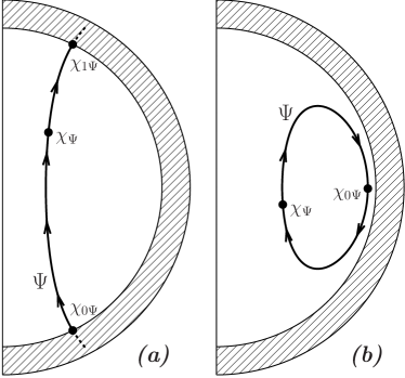
Figure 1: Meridional cross-sections of an NS. Straight vertical lines show the symmetry axis of the star. Hatched regions show the NS crust, white regions show the core. The poloidal magnetic field lines are depicted by the thick black lines (lie on the surface of constant $\Psi$). A direction of the field is shown by arrows and coincides with the direction of integration in Eqs. (45), (46), and (47). (a) The field line with a given $\Psi$ is open in the core. The initial point $\chi_{0\Psi}$ coincides with the point, where the field line enters the core. A point where the field line leaves the core is denoted as $\chi_{1\Psi}$. (b) The field line with a given $\Psi$ is closed in the core. The starting point $\chi_{0\Psi}$ is defined as the nearest point to the crust.

There are two possibilities. The first one is that the field line is open in the core (Fig. 1a) and has two points where it crosses the crust-core interface. Here we do not care whether this line closes up in the crust or continues to the magnetosphere. Let $\chi_{0\Psi}$ be a point where the field line enters the core from the crust, and $\chi_{1\Psi}$ be a point where the field line leaves the core. There should be a boundary condition at $\chi_{1\Psi}$ similar to that at the point $\chi_{0\Psi}$, namely, $U_{b\varphi}/(r\sin\theta)|_{\chi_{1\Psi}}=\Omega_{1}(\Psi,t)$. Then we have for $I^{\prime}_{t}(\Psi,\,t)$ (see Eq. 45)

$$I^{\prime}_{t}(\Psi,t)=\left(\int_{\chi_{0\Psi}}^{\chi_{1\Psi}}\frac{(\boldsymbol{\nabla}\varphi)^{2}}{B^{(p)}}\mathrm{d}\chi\right)^{-1}\left(\Omega_{1}(\Psi,t)-\Omega_{0}(\Psi,t)+G\bigr{|}_{\chi_{0\Psi}}^{\chi_{1\Psi}}+\int_{\chi_{0\Psi}}^{\chi_{1\Psi}}\frac{F}{B^{(p)}}\mathrm{d}\chi\right).$$ (46a)

The second option is realized if the field line is closed up in the core (Fig. 1b). Integrating then Eq. (45) over the closed loop along the field line shown in Fig. 1b, we obtain

$$I^{\prime}_{t}(\Psi,t)=\left(\oint_{\Psi}\frac{(\boldsymbol{\nabla}\varphi)^{2}}{B^{(p)}}\mathrm{d}\chi\right)^{-1}\oint_{\Psi}\frac{F}{B^{(p)}}\mathrm{d}\chi.$$ (46b)

Note that there is no way to relate the “boundary” function $\Omega_{0}(\Psi,t)$ to that in the crust in the case of closed field lines. The region in the core, where the field lines are closed up, appears to be magnetically decoupled from the rest of the star. This seems to be in line with the results of Ref. Glampedakis and Lasky (2015), although the arguments presented there are quite different.

Note also that for a magnetic field configuration with equatorial symmetry one has $\Omega_{1}(\Psi,\,t)=\Omega_{0}(\Psi,\,t)$ and $G|_{\chi_{1\Psi}}=G|_{\chi_{0\Psi}}$, and consequently $I^{\prime}_{t}(\Psi,t)$ is independent of the “boundary” functions $\Omega_{0}(\Psi,\,t)$ and $\Omega_{1}(\Psi,\,t)$ (cf. Eq. 46a),

$$I^{\prime}_{t}(\Psi,t)=\left(\int_{\chi_{0\Psi}}^{\chi_{1\Psi}}\frac{(\boldsymbol{\nabla}\varphi)^{2}}{B^{(p)}}\mathrm{d}\chi\right)^{-1}\int_{\chi_{0\Psi}}^{\chi_{1\Psi}}\frac{F}{B^{(p)}}\mathrm{d}\chi.$$ (47)

Summarizing, we have a recipe to derive the function $I^{\prime}_{t}(\Psi,\,t)$ in Eq. (45). Therefore, we can calculate $U_{b\varphi}$ for a given magnetic field configuration.

III.6 Summary of results for Sec. III

To calculate the fluid motions induced by the magnetic field one should:

(i) determine $\Delta\mu$ and $\delta\mu_{n}$ from Eqs. (25) and (30) with the boundary conditions (31) and (33);

(ii) calculate $\boldsymbol{U}_{b}^{(p)}$ from Eqs. (18) and (20), and $\boldsymbol{U}_{b}^{(t)}$ from Eqs. (45) and (46);

(iii) if one also needs the particle species velocities $\boldsymbol{u}_{a}$ one should first calculate the diffusion velocities $\boldsymbol{w}_{a}$ from Eqs. (11) and then use the formula $\boldsymbol{u}_{a}=\boldsymbol{U}_{b}+\boldsymbol{w}_{a}$.

Moreover, from Eqs. (38) and (46) we now know the time derivatives $\partial\Psi/\partial t$ and $I^{\prime}_{t}(\Psi,\,t)$, which opens up a possibility to determine the derivative $\partial\boldsymbol{B}/\partial t$ for arbitrary $\boldsymbol{B}$, and hence to model the magnetic field evolution in a fully self-consistent way.

IV Quasistationary particle flows: numerical results

The general formalism developed in the previous section allows one to calculate particle velocities in a nonsuperfluid magnetized $npe$-cores of NSs. In this section we present an example of such calculation for two simple models of the poloidal magnetic field, and discuss the main properties of the obtained solutions.

We adopt the same microphysical inputs as in our previous work Gusakov et al. (2017). Namely, we consider an NS with the mass $M=1.4\,$M_⊙ and assume $npe$ HHJ equation of state in the core from Ref. Heiselberg and Hjorth-Jensen (1999). Such an NS model has a radius $R=12.2$ km and the core radius $R_{\rm core}=11.2$ km. To calculate the unperturbed quantities as functions of the radial coordinate $r$ [e.g., the number densities, $n_{a}(r)$] we, somewhat inconsistently, use fully relativistic Tolman-Oppenheimer-Volkoff equations Oppenheimer and Volkoff (1939); Tolman (1939), although perturbed equations are treated in the Newtonian framework. Such an approach allows us to obtain reasonable NS radii, while keeping the discussion of the magnetic field effects relatively simple. We do not expect that accurate account for General Relativity effects will affect our results qualitatively.

To calculate the friction coefficients, $J_{ep}$ and $J_{np}$, we employ equations (78) and (79) from Ref. Gusakov et al. (2017). In turn, the reaction rate $\Delta\Gamma$, which is generated by the modified Urca processes is taken from Ref. Yakovlev et al. (2001) (the more powerful direct Urca process is forbidden for the chosen NS configuration). All these quantities depend on the local stellar temperature $T$, which is related to the redshifted stellar temperature $\widetilde{T}$ by the formula: $T=\widetilde{T}/\sqrt{g_{00}}$, where $g_{00}(r)$ is the time component of the metric tensor. Because of high thermal conductivity (see, e.g., Ref. Potekhin et al. (2015)), the cores of not too young NSs can be treated as nearly isothermal, $\widetilde{T}=\mathrm{const}$, which makes $\widetilde{T}$ a convenient parameter to characterize the thermal state of our system (see below).

IV.1 “Minimal” model of the magnetic field

Following Refs. Akgün et al. (2013); Passamonti et al. (2017) we start with the simplest analytic expression fo the poloidal flux function,

$$\Psi(r,\theta)=B_{\text{max}}R^{2}f\left(\frac{r}{R}\right)\sin^{2}\theta,$$ (48)

where $B_{\text{max}}$ is the maximum value of the magnetic field inside the star; $R$ is the NS radius; and $f(x)$ is the analytic function to be specified below. In the axisymmetric case the field near the stellar centre should be almost homogeneous and aligned with the symmetry axis. Thus at $x=r/R\ll 1$ we should have $f\sim x^{2n}$, where $n\geq 1$ (the case $n=0$ is excluded by the regularity requirement of the magnetic field at $x\rightarrow 0$). Assuming, as was suggested in Ref. Akgün et al. (2013), that $f$ inside the star takes the form, $f=\sum_{n\geq 1}f_{2n}\,x^{2n}$, and matching this expression with the vacuum dipole field outside the star ($f\propto 1/x$), we obtain Passamonti et al. (2017)

$$f(x)=\frac{1}{2}x^{2}-\frac{3}{5}x^{4}+\frac{3}{14}x^{6}.$$ (49)

This is a minimal solution for $f(x)$ in the domain $x\in[0,1]$, satisfying the requirements

$$f^{\prime}(1)=-f(1),\qquad f^{\prime\prime}(1)=2f(1).$$ (50)

The first of these conditions is necessary for continuity of the magnetic field, while the second one ensures that the charge current density at the surface vanishes (see, e.g., Ref. Passamonti et al. (2017) for more details). The expression (49) differs from that proposed in equation (30) of Ref. Passamonti et al. (2017) by a numerical factor $35/4$, appearing due to a different normalization. The magnetic field $\boldsymbol{B}=\boldsymbol{B}^{(p)}$, corresponding to $f(x)$ from Eq. (49), is shown in Fig. 3.

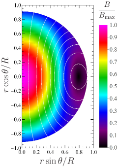
Figure 2: A meridional cross-section of an NS core and “minimal” configuration of the magnetic field considered in the text. Field lines are shown by white curves. The strength of the magnetic field is denoted by different colors.

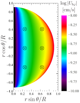
Figure 3: The toroidal component of the baryon velocity $U_{b\varphi}$ for the minimal magnetic field model. Colors denote the value of $U_{b\varphi}$ in the logarithmic scale (in cm/s). Crossed circles represent the direction of $U_{b\varphi}$ (cf. Fig. 9c).

Now let us turn to the toroidal (azimuthal) velocity $U_{b\varphi}$. It is interesting that $U_{b\varphi}$ can be easily calculated for a purely poloidal field (when the poloidal current function $I=0$). Then, according to Eqs. (41) and (61), one has $F=0$ and $G=-j_{\varphi}/(en_{e}r\sin\theta)$; the function $I^{\prime}_{t}(\Psi,\,t)$ also vanishes because of the equatorial symmetry of the chosen magnetic field (see Eq. 47). Hence, $U_{b\varphi}$ can be found provided that the “boundary” function $\Omega_{0}(\Psi,\,t)$ is known (see Eq. 45). Generally, $\Omega_{0}(\Psi,\,t)$ can only be determined from the joint solution to the full system of the magnetic evolution equations in the crust and core. Here we do not attempt to find such a solution and instead, for illustration, assume that $\Omega_{0}(\Psi)=-G|_{\chi_{0\Psi}}$. Then

$$U_{b\varphi}=\frac{j_{\varphi}}{en_{e}}=-\frac{c}{4\pi en_{e}\,r{\rm sin}\,\theta}\Delta{\!\!}^{*}\Psi;$$ (51)

the result is plotted in Fig. 3. Note that $U_{b\varphi}$ does not explicitly depend on the NS temperature and is proportional to $B_{\rm max}$. Note also that, with our choice of boundary condition for $U_{b\varphi}$, it follows from Eqs. (11c) and (51) that $U_{b\varphi}$ is related to the $\varphi$-component of the electron diffusion velocity $\boldsymbol{w}_{e}$ by the formula,

$$U_{b\varphi}=-w_{e\varphi}.$$ (52)

IV.2 Chemical potential perturbations

Now let us discuss how the application of the method, outlined in Secs. III.3 and III.4, works for calculation of the chemical potential perturbations, $\delta\mu_{n}$ and $\Delta\mu$.

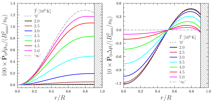
Figure 4: Radial dependence of the zeroth-order Legendre components of (rescaled) chemical potential perturbations, $100\times\delta\mu_{n}/(B_{\text{max}}^{2}/n_{0})$ and $10\times\Delta\mu/(B_{\text{max}}^{2}/n_{0})$, for the minimal magnetic field model from Sec. IV.1. Colored lines show the exact solution to Eqs. (30) with the boundary conditions (31) and (33b) for a set of redshifted temperatures indicated in the figure. Dashed lines are plotted in the low-temperature limit (almost coincide with the black lines); dot-dashed lines illustrate the high-temperature limit. Hatched regions correspond to the crust, where our approach is invalid.

Colored lines in Fig. 4 display solutions to Eqs. (30) for the quantities $\hat{\bf P}_{0}\delta\mu_{n}$ and $\hat{\bf P}_{0}\Delta\mu$ with the boundary conditions (31) and (33b), for a number of redshifted stellar temperatures $\widetilde{T}$, listed in the figure. For a sufficiently weak magnetic field, departure of the system from the beta-equilibrium state is small, $\Delta\mu\ll\pi kT$, hence one can present $\Delta\Gamma$ as Gusakov et al. (2017): $\Delta\Gamma=\lambda\Delta\mu$ (the subthermal regime). Consider the system in this regime. Then the differential equations (30) become linear, and, as a result, $\hat{\bf P}_{0}\delta\mu_{n}$ and $\hat{\bf P}_{0}\Delta\mu$ both proportional to $B_{\text{max}}^{2}$, because $\hat{\bf P}_{0}f_{Ar}\propto B_{\text{max}}^{2}$. Thus, the dimensionless combinations $100\times\hat{\bf P}_{0}\delta\mu_{n}/(B_{\text{max}}^{2}/n_{0})$ and $10\times\hat{\bf P}_{0}\Delta\mu/(B_{\text{max}}^{2}/n_{0})$ ($n_{0}=0.16\,$fm^-3 is the nuclear saturation density), which are shown in Fig. 4, are independent of $B_{\text{max}}^{2}$.

Dashed and dot-dashed lines show, respectively, the low-temperature and high-temperature limits for $\hat{\bf P}_{0}\delta\mu_{n}$ and $\hat{\bf P}_{0}\Delta\mu$ (see details in Sec. III.4). One can see that the temperature $\widetilde{T}=2\times 10^{8}\,$K is small enough to imitate the low-temperature limit (black lines in Fig. 4 almost coincide with the dashed ones). At $\widetilde{T}\sim 3.5\times 10^{8}\,$K the solution to Eqs. (30) is equally far from both limits. The highest $\widetilde{T}$, for which we numerically solved Eqs. (30), was $\widetilde{T}=5\times 10^{8}\,$K. This value is close to the high-temperature limit, but still significantly differs from it. At higher $\widetilde{T}$ Eq. (30a) becomes poorly conditioned so that numerical integration of the system (30) is complicated.

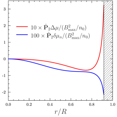
Figure 5: The same as in Fig. 4, but for the second-order Legendre components of $\delta\mu_{n}$ and $\Delta\mu$.

The flux function (48) contains two Legendre components, $P_{0}(\cos\theta)$ and $P_{2}(\cos\theta)$. The same is true for the chemical potential perturbations. Fig. 5 shows dimensionless combinations $100\times\hat{\bf P}_{2}\delta\mu_{n}/(B_{\text{max}}^{2}/n_{0})$ and $10\times\hat{\bf P}_{2}\Delta\mu/(B_{\text{max}}^{2}/n_{0})$ as functions of radial coordinate. According to Eq. (25), these combinations do not depend on $B_{\text{max}}^{2}$ and are fully determined by the magnetic field. Typically, $\hat{\bf P}_{2}$-components are comparable to $\hat{\bf P}_{0}$-components in the major part of the core. However, there is a rapid (but finite) growth of $\hat{\bf P}_{2}\delta\mu_{n}$ and $\hat{\bf P}_{2}\Delta\mu$ near the crust-core interface. The reason for that is a substantial softening of EOS at $n_{b}\lesssim n_{0}$, which results in large derivatives $n^{\prime}_{b}$ and $n^{\prime}_{e}$ in the vicinity of the crust-core boundary. This effect is generic (should be present for all EOSs), as is argued in Appendix C.

Now let us discuss what happens if the system is in the regime, in which $\Delta\mu\gtrsim\pi kT$ (suprathermal regime). In this case $\Delta\Gamma$ is a polynomial in $\Delta\mu/\pi kT$ Reisenegger (1995b). As follows from Figs. 4 and 5, a typical absolute value of the chemical potential imbalance is $\sim(0.03-0.1)\times B_{\text{max}}^{2}/n_{0}$. Correspondingly, a typical magnetic field $B_{\text{max}}^{\star}$ for the transition of the system into the suprathermal regime is given by

$$B_{\text{max}}^{\star}\sim(0.8-1.5)\times 10^{16}\sqrt{\frac{T}{10^{8}\,\text{K}}}~{}{\rm G}.$$ (53)

Note that this equation depends on the local temperature $T$, which is greater than the redshifted one. In the deepest layers of the core $T$ can be larger than $\widetilde{T}$ by a factor of $\sim 1.5$. Then for a typical magnetar temperature Beloborodov and Li (2016), $\widetilde{T}\sim 2\times 10^{8}\,$K, one can expect $B_{\text{max}}^{\star}>10^{16}\,$G. Such a large field can be reached in magnetars, but in what follows we prefer to avoid nonlinearities in $\Delta\Gamma$ by choosing $B_{\text{max}}=5\times 10^{15}\,$G.

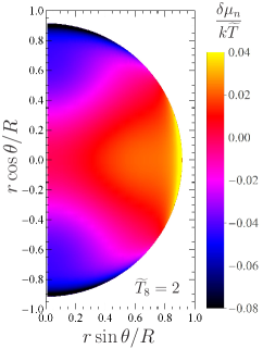
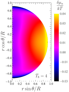
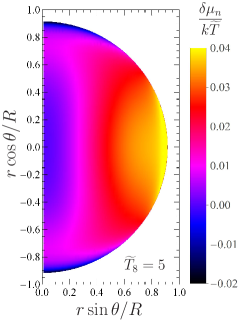
Figure 6: Two-dimensional density plot showing the ratio of $\delta\mu_{n}/(k\widetilde{T})$ in the star for the minimal model of the magnetic field with $B_{\text{max}}=5\times 10^{15}\,$G. The left, middle, and right panels are plotted for $\widetilde{T}=2\times 10^{8}\,$K, $4\times 10^{8}\,$K, and $5\times 10^{8}\,$K, respectively.

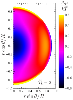
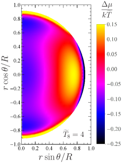
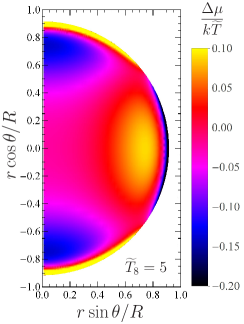
Figure 7: The same as in Fig. 6 but for the ratio $\Delta\mu/(k\widetilde{T})$ and $\widetilde{T}=2\times 10^{8}\,$K (left panel), $\widetilde{T}=4\times 10^{8}\,$K (middle panel), and $\widetilde{T}=5\times 10^{8}\,$K (right panel); see the text.

Our calculations are illustrated in Figs. 6 and 7, where we present density plots for the ratios $\delta\mu_{n}/(k\widetilde{T})$ and $\Delta\mu/(k\widetilde{T})$. One sees from Fig. 6 that the second-order Legendre component of $\delta\mu_{n}$ dominates the zeroth one at $\widetilde{T}=2\times 10^{8}\,$K; at $\widetilde{T}=4\times 10^{8}\,$K and $5\times 10^{8}\,$K they are comparable, with a tendency that $\hat{\bf P}_{0}$-component becomes more and more important with increasing $\widetilde{T}$. The situation with the chemical potential imbalance $\Delta\mu$ is reversed (Fig. 7). At $\widetilde{T}=2\times 10^{8}\,$K the zeroth-order Legendre component, $\hat{\bf P}_{0}\Delta\mu$, is slightlylarger than $\hat{\bf P}_{2}\Delta\mu$, but this difference smooths out at $\widetilde{T}=4\times 10^{8}\,$K; finally, at $\widetilde{T}=5\times 10^{8}\,$K the second-order component dominates.

IV.3 Poloidal flows in the minimal-field model

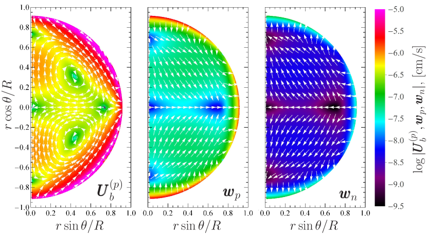
Figure 8: Two dimensional density plots showing the (logarithm of) poloidal component of the baryon velocity $\boldsymbol{U}_{b}^{(p)}$ (left panel), the proton diffusion velocity $\boldsymbol{w}_{p}$ (middle panel), and the neutron diffusion velocity $\boldsymbol{w}_{n}$ (right panel) for the minimal magnetic field model with $B_{\text{max}}=5\times 10^{15}\,$G and $\widetilde{T}=2\times 10^{8}\,$K. Arrows indicate the velocity direction.

In what follows we consider a neutron star with $\widetilde{T}=2\times 10^{8}\,$K and $B_{\text{max}}=5\times 10^{15}\,$G. The chosen $\widetilde{T}$ corresponds to the low-temperature limit, $\varkappa\gg 1$, as discussed in Sec. IV.2 (see the end of Sec. III.4 for a definition of $\varkappa$). Then one has $\hat{\bf P}_{0}\mu_{n}=0$; in addition, the condition $\varkappa\gg 1$ together with the estimate from the footnote 7 allow us to neglect the rate $\Delta\Gamma$ in Eq. (18). This significantly simplifies calculation of the poloidal component $\boldsymbol{U}_{b}^{(p)}$ of the baryon velocity, as well as the proton and neutron diffusion velocities, $\boldsymbol{w}_{p}$ and $\boldsymbol{w}_{n}$.

Fig. 8 presents these three quantities. Note that, for purely poloidal field $\boldsymbol{B}$ the poloidal projections of $\boldsymbol{w}_{p}$ and $\boldsymbol{w}_{e}$ coincide, while $w_{e\varphi}=-U_{b\varphi}$ (see Eq. 52). One can see that the poloidal component $\boldsymbol{U}_{b}^{(p)}$, generated by the magnetic field, is rather high, $U_{b}^{(p)}\sim(0.3-1)\times 10^{-6}\,$cm/s, and it rapidly increases near the crust-core interface. It is also much larger than the typical diffusion velocities and the component $U_{b\varphi}$ (see Fig. 3). Typically, $\boldsymbol{U}_{b}^{(p)}$ in the core can be estimated as (for a given model of the magnetic field)

$$U_{b}^{(p)}\sim(10-30)\,w_{p},$$ (54)

while the proton and neutron diffusion velocities are related by the formula, $\boldsymbol{w}_{p}=-(n_{n}/n_{e})\boldsymbol{w}_{n}$ (see Eq. 11), and thus $w_{p}\sim 10w_{n}$. Note that the relation (54) remains valid in a wide range of $\widetilde{T}$ (low enough to neglect $\Delta\Gamma$) and $B_{\text{max}}$, since all the three velocities $\boldsymbol{U}_{b}^{(p)}$, $\boldsymbol{w}_{p}$, and $\boldsymbol{w}_{n}$ scale as $\propto B_{\text{max}}^{2}/\widetilde{T}$. The reason why $\boldsymbol{U}_{b}^{(p)}$ is much larger than $\boldsymbol{w}_{p}$ and $\boldsymbol{w}_{n}$ can be explained as follows. Let us express, for example, $\theta$-component, $U_{b\theta}$, of the baryon velocity through $\boldsymbol{w}_{p}$. Using Eqs. (11b), (18), and (20), one can write

$$U_{b\theta}=\frac{1}{n_{b}r\,{\rm sin}\theta}\,\frac{\partial}{\partial r}\left(\frac{r^{2}}{x_{e}^{\prime}}\int_{0}^{\theta}{\rm div}(n_{e}\boldsymbol{w}_{p})\,{\rm sin}\tilde{\theta}\,d\tilde{\theta}\right),$$ (55)

where $x_{e}\equiv n_{e}/n_{b}$. Naive estimate of this expression, which assumes $d/dr\sim 1/R$, suggests, incorrectly, that $U_{b\theta}\sim w_{p}$. What is wrong here? Note that $\boldsymbol{w}_{p}$ depends on various derivatives of $n_{b}$ and $n_{e}$, as well as on the derivatives of the magnetic function $f(r/R)$ (see Eqs. 11b and 25), namely, on $n_{b}^{\prime}$, $n_{e}^{\prime}$, $n_{b}^{\prime\prime}$, $n_{e}^{\prime\prime}$, $f$, $f^{\prime\prime}$, and $f^{\prime\prime\prime}$. Correspondingly, $U_{b\theta}$ depends on up to the fourth derivative of $n_{b}$ and $n_{e}$ and up to fifth derivative of $f$ (see Eq. 55). These derivatives can be very large, so that, for example, an estimate $n_{b}^{\prime\prime\prime\prime}(r)\sim n_{b}^{\prime\prime}(r)/R^{2}$ simply does not work; instead we have $n_{b}^{\prime\prime\prime\prime}(r)\gg n_{b}^{\prime\prime}(r)/R^{2}$ in the outer layers of NS cores. The reason for that is discussed in Appendix C, where we, using as an example the $|n_{b}^{\prime}/(n_{b}/R)|$ ratio, demonstrate that the derivatives are especially large near the crust-core interface, where the stellar density rapidly decreases with $r$. In turn, the fact, that $U_{b\theta}$ depends on up to the fifth derivative of the function $f$ indicates that baryon velocity can be extremely sensitive to the model of the magnetic field inside the NS core. Note, in this respect, that the model (48), used by us here, is one of the smoothest (the magnetic field has a maximum at the stellar centre and then decreases monotonically in the direction of the crust, see Fig. 3). We expect (and we checked it numerically for a number of different magnetic field configurations) that for less smooth models the baryon velocity will generally be even larger. Summarizing, the above consideration suggests that ${\boldsymbol{U}}_{b}$ will exceed the diffusion velocities for a wide class of magnetic field geometries, except, perhaps, for some very specific configurations, in which large-derivative terms cancel each other out (see also Sec. V).

Since $\boldsymbol{U}_{b}$ dominates the diffusion velocities, all particle species move almost as a single fluid, $\boldsymbol{u}_{a}=\boldsymbol{U}_{b}+\boldsymbol{w}_{a}\approx\boldsymbol{U}_{b}$. Using the expression (11b), it is easy to estimate various terms in Eq. (12) and verify that the main contribution to $\delta\boldsymbol{E}_{\text{com}}$ comes from the third term in the right-hand side of Eq. (12), so that $\delta E_{\text{com}}\sim(w_{p}/c)B\sim 0.05|(\boldsymbol{U}_{b}^{(p)}/c)\times\boldsymbol{B}|$. Correspondingly, the magnetic field lines are “frozen-in” to the $npe$-plasma to a good approximation (see Eq. 9),

$$\frac{\partial\boldsymbol{B}}{\partial t}\approx\operatorname{curl}\left(\boldsymbol{U}_{b}\times\boldsymbol{B}\right).$$ (56)

An interesting feature of the solution presented in Fig. 8 is non-vanishing neutron and proton flows through the crust-core interface. Although these flows conserve total number of neutrons and protons in the core and, generally, cannot be excluded on physical grounds, it looks a bit strange that they appear inevitably in our scheme (for a given magnetic field configuration) and we do not have enough freedom to “kill” them, e.g., by tuning in the boundary conditions at the interface. The question is what, effectively, plays the role of a “boundary condition” at the crust-core interface? We believe it is the magnetic field itself, which, together with the quasistationarity assumption, encodes all information about the particle flows through the interface. To illustrate this point, in the next section we build up a magnetic field model, which prevents baryons from moving into the crust.

IV.4 A magnetic field model with no baryon current through the crust-core interface

There is no baryon currents through the crust-core interface if $u_{nr}|_{R_{\text{core}}}=u_{pr}|_{R_{\text{core}}}=0$. This requirement can be reformulated in terms of the velocities $\boldsymbol{U}_{b}$, $\boldsymbol{w}_{p}$ and $\boldsymbol{w}_{n}$ as: $U_{br}|_{R_{\text{core}}}=0$ and $w_{pr}|_{R_{\text{core}}}=w_{nr}|_{R_{\text{core}}}=0$. Employing Eqs. (11a) and (11b), the latter condition can be rewritten as

$$\left(\hat{\bf P}_{l}\delta\mu_{n}\right)^{\prime}\Bigr{|}_{R_{\text{core}}}=0,\quad l\geqslant 0.$$ (57)

Note that Eq. (57) for $l=0$ is automatically satisfied due to the boundary condition (33b). Using Eq. (20) for $\boldsymbol{U}_{b}^{(p)}$, the condition $U_{br}|_{R_{\text{core}}}=0$ is equivalent to $\hat{\bf P}_{l}V|_{R_{\text{core}}}=0$ for each $l\geqslant 0$ (for $l=0$ this condition should already be satisfied, as explained in Sec. III.3). In the low-temperature limit we are interested in here, we may omit the reaction rate $\Delta\Gamma$ in Eq. (18) for $V$. Then the condition $\hat{\bf P}_{l}V|_{R_{\text{core}}}=0$ can be represented as

$$\left[\left(\hat{\bf P}_{l}\delta\mu_{n}\right)^{\prime\prime}-\frac{l(l+1)}{r^{2}}\hat{\bf P}_{l}\delta\mu_{n}\right]\Biggr{|}_{R_{\text{core}}}=0,\quad l\geqslant 1,$$ (58)

where we have used Eq. (57). Substituting the expressions (25) for $\delta\mu_{n}$ into Eqs. (57) and (58), we arrive at the two conditions for the Ampere force, $\boldsymbol{f}_{A}$. Using Eq. (63), these conditions can be written in terms of the flux and current functions, $\Psi$ and $I$.

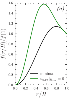
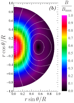
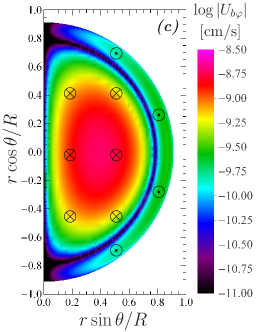
Figure 9: (a) Comparison of the dimensionless functions $f$ for the minimal magnetic field model from Sec. IV.1 (black line) and for the model of Sec. IV.4 (green line). (b) Magnetic field model from Sec. IV.4 (cf. Fig. 3). (c) Density plot for the toroidal component of the baryon velocity for the magnetic field model from Sec. IV.4 (cf. Fig. 3). Circles with crosses and dots indicate direction of the toroidal component.

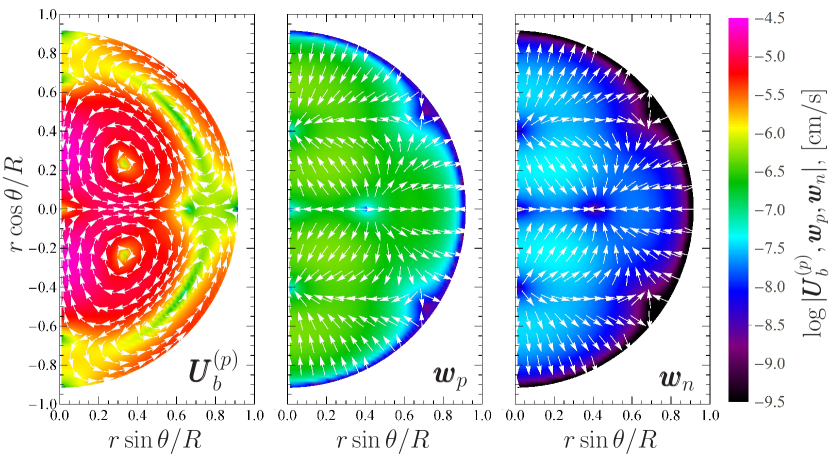
Figure 10: The same as in Fig. 8, but for the magnetic field model from Sec. IV.4

In the case of a purely poloidal field with simple angular dependence (48) of the function $\Psi$, the conditions (57) and (58) are nontrivial only for the Legendre component with $l=2$. Thus, we have two new conditions for the function $f(x)$ and the three old conditions, namely Eq. (50) and the normalization. A simple (numerical) solution, satisfying these conditions, reads (five coefficients in the formula are needed to satisfy 5 conditions)

$$f=0.5x^{2}-1.557x^{4}+2.113x^{6}-1.358x^{8}+0.338x^{10}.$$ (59)

In Fig. 9a we compare this function with $f(x)$ for the minimal-field model (see Eq. 49). Both models look similar, as is also confirmed by Fig. 9b, presenting the new magnetic field model. It resembles Fig. 3 with the only difference that now $\boldsymbol{B}$ is more “compressed” to the central regions of the core. The main difference concerns the toroidal component of the baryon velocity (Fig. 9c), which has a more complicated topology comparing to $U_{b\varphi}$ for the minimal model of the magnetic field (Fig. 3).

Fig. 10 shows the baryon and diffusion velocities for the new model of the magnetic field. We see that this field indeed suppresses all radial velocities at the crust-core interface. However, the $U_{b\theta}$ component near $r=R_{\text{core}}$ does not vanish. The structure of the flows significantly differs from what we see in Fig. 8. In particular, we have four curls in Fig. 10 (left panel) instead of two, as in the minimal-field model. Average absolute values of the velocities are plotted in Fig. 10 and appear to be about one order of magnitude larger than in Fig. 8. However, the scaling relation (54) remains unaltered.

V Discussion & Conclusions

In our previous paper Gusakov et al. (2017) we proposed a self-consistent method to explore the magnetic field evolution in NS cores. The main attractive feature of the method is that it does not assume, from the very beginning, that the neutron or baryon velocities are small or vanish (as, e.g., in Refs. Goldreich and Reisenegger (1992); Thompson and Duncan (1996); Glampedakis et al. (2011b); Graber et al. (2015); Passamonti et al. (2017)), but instead provide a receipt to calculate them. In the present paper we further developed this method and applied it to the model of a nonsuperfluid and nonsuperconducting NS, whose core consists of neutrons, protons, and electrons. Such a NS model may adequately describe hot, high-$B$ magnetars with partially or fully suppressed baryon superfluidity in their cores Sinha and Sedrakian (2015); Sedrakian et al. (2017). Our main result is the calculation of particle velocities in the NS core, generated by the presence of the magnetic field.

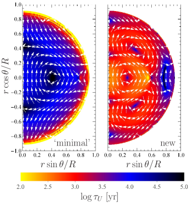
Figure 11: Density plot showing the logarithm of the timescale $\tau_{U}$ (in yr) for the minimal model of the magnetic field from Sec. IV.1 (left panel) and for the model with no particle flows through the crust-core interface from Sec. IV.4 (right panel). Arrows indicate direction of the derivative $\partial\boldsymbol{B}/\partial t$ given by Eq. (56). To plot the figure we assumed $B_{\rm max}=5\times 10^{15}$ G and $\widetilde{T}=2\times 10^{8}$ K.

There are several interesting properties of our solution which, as we argue in Sec. IV.3, should be common to a wide class of magnetic-field models (see also a discussion below). First and most importantly, we showed that neutrons, protons, and electrons in the core move almost as a single fluid, i.e., the diffusion velocities $\boldsymbol{w}_{a}$ ($a=n$, $p$, $e$) are much smaller than the baryon velocity $\boldsymbol{U}_{b}$ (see Eq. 7). This result contradicts the statement that neutrons (or baryons) in NSs are motionless to a good approximation (e.g., Refs. Goldreich and Reisenegger (1992); Thompson and Duncan (1996); Beloborodov and Li (2016); Passamonti et al. (2017); Castillo et al. (2017)). Specifically, we showed, for the two models of the magnetic field discussed in Sec. IV, that for charged particles $w_{p,e}=|\boldsymbol{u}_{p,e}-\boldsymbol{U}_{b}|\sim 0.05U_{b}$, while for neutrons $w_{n}=|\boldsymbol{u}_{n}-\boldsymbol{U}_{b}|\sim 0.005U_{b}$. Note that here the factors in front of $U_{b}$ depend sensitively on the magnetic field model and can be made substantially smaller for a less “smooth” magnetic function $f(x)$ (see Sec. IV.3).

The second property is that, typically, the velocity $\boldsymbol{U}_{b}$ is rather high and it rapidly increases in the outer layers of the core. For example, $U_{b}\sim(0.3-1)\times 10^{-6}$ cm/s for the magnetic field model with $B_{\text{max}}=5\times 10^{15}$ G and temperature $\widetilde{T}=2\times 10^{8}$ K. On the other hand, the particle velocities $\boldsymbol{u}_{a}$ and $\boldsymbol{U}_{b}$ scale similarly with $B_{\text{max}}$ and $\widetilde{T}$ in the low- and high-temperature regimes (see Sec. IV.2), thus $\boldsymbol{U}_{b}$ will remain much larger than the diffusion velocities $\boldsymbol{w}_{a}$ if this is the case for some particular values of $B_{\rm max}$ and $\widetilde{T}$.

Another interesting property of our solution is that some magnetic field configurations can lead to neutron and proton flows through the crust-core interface. Although, generally, we see no reasons why such behavior is impossible, we derived a set of conditions (Sec. IV.4) on the magnetic field, preventing these particle species from penetrating the crust, and found a magnetic field model, satisfying these requirements. Note that the “minimal” model of Refs. Passamonti et al. (2017); Akgün et al. (2013) is not compatible with these requirements.

The solution that we have just discussed was obtained for two specific models of the magnetic field. But how representative are these models? In Sec. IV.3 we argue that the main feature of our solution — large baryon velocity ${\boldsymbol{U}}_{b}$, exceeding the diffusion velocities ${\boldsymbol{w}}_{a}$ — is inherent in a wide class of magnetic-field models [see a discussion after Eq. (55)]. This is because ${\boldsymbol{U}}_{b}$ depends on high spatial derivatives of the magnetic field and number densities, which can be very large. Of course, one can imagine a “fine-tuned” model (or a set of models), in which these large derivatives cancel each other out, so that the resulting ${\boldsymbol{U}}_{b}$ is comparable to the diffusion velocities. But what is the probability that such a model is realized in an NS, for instance, at its birth? The magnetic field of a newly-born star is determined by the way it is generated in the process of NS formation. It knows nothing about what model leads or does not lead to large ${\boldsymbol{U}}_{b}$. Therefore, we expect that the probability to have a “fine-tuned” magnetic-field configuration for a young NS is negligible.

However, one cannot exclude that the magnetic field may converge to the “fine-tuned” configuration during the NS evolution. This will happen if the models with $U_{b}\sim w_{a}$ constitute an attractor for our problem, in analogy with the Hall attractor in the NS crust Gourgouliatos and Cumming (2014a). Note that, for this scenario to work, the magnetic field configuration corresponding to the attractor state should be dynamically stable. Otherwise, approaching the attractor, the magnetic field will reconfigure on the Alfven timescale to some other (stable) configuration (most likely, with large ${\boldsymbol{U}}_{b}$), and the cycle of quasistationary evolution starts over again. Whether these scenarios are realized in reality is an open question that needs further investigation.

If the configuration of the magnetic field is such that the NS matter moves almost as a single fluid (i.e., $U_{b}>w_{a}$), then ${\boldsymbol{B}}$ is (approximately) frozen-in to the $npe$-plasma, so that the field lines are dragged with it [see Eq. (56)]. This introduces a new timescale into the problem (not to be confused with the dissipation timescale studied in Ref. Gusakov et al. (2017)!), associated with the drag velocity ${\boldsymbol{U}}_{b}$, $\tau_{U}=B/|\operatorname{curl}(\boldsymbol{U}_{b}\times\boldsymbol{B})|$. The timescale is plotted in Fig. 11 for the two models of the magnetic field discussed in the text. To plot the figure we assumed $B_{\rm max}=5\times 10^{15}$ G and $\widetilde{T}=2\times 10^{8}$ K, but the result can be easily rescaled to any $B_{\rm max}$ and $\widetilde{T}$ since $\tau_{U}\propto B_{\rm max}^{2}/\widetilde{T}^{2}$ for $\widetilde{T}\lesssim 3\times 10^{8}$ K. One sees, that for the minimal magnetic field model (left panel) $\tau_{U}\sim 10^{4}$ yr in the bulk of the core, but becomes much smaller, $\lesssim 10^{2}$ yr, in the vicinity of the crust. The behavior of $\tau_{U}$ for the model with suppressed particle flows through the crust-core boundary (right panel) is quite different: $\tau_{U}$ for that model is $\sim 10^{3}$ yr in the major part of the core. It seems plausible that the real timescale $\tau$ for the magnetic field evolution in the star will be closer to the minimal value of $\tau_{U}$, i.e., $\tau\sim 10^{2}$ yrs for the model of Sec. IV.1 and $\tau\sim 10^{3}$ yrs for the model of Sec. IV.4. In both cases $\tau$ is noticeably smaller than the typical magnetar age, $\sim 10^{4}$ yr Olausen and Kaspi (2014). This observation suggests a principal possibility that reconfiguration of the magnetic field in the core may be responsible for violent magnetar activity during its lifetime, or even may lead to (repeating) fast radio bursts Popov and Postnov (2013); Beloborodov (2017); Popov et al. (2018).

Of course, we are still far from the final solution to the problem of the magnetic field evolution in NS interiors. Now we are able just to find all the necessary ingredients in order to calculate the derivative $\partial\boldsymbol{B}/\partial t$ for a simplest model of an NS and for a predefined model of the magnetic field. The next steps, therefore, could be (i) to solve the Faraday’s equation to see how the magnetic field evolves in time and (ii) to extend the results obtained here to more realistic (and complex) models of NSs. To reach the goal (i) one needs, first of all, to include the crust into consideration, to obtain a quasistationary solution for the magnetic field there, and then to match both solutions in the crust and core, allowing for possible particle currents through the crust-core interface. In turn, the goal (ii) assumes a lot of work. One needs to take into account general relativity effects in MHD equations (which should not affect the results quantitatively), to consider various core compositions (not only $npe$-matter), but the most important task will be to extend our consideration to superfluid and superconducting matter. Such an extension is absolutely necessary for modeling radio and millisecond pulsars, and it can be done along the lines reviewed in Ref. Gusakov et al. (2017). Our preliminary results indicate that account for nucleon pairing has a tendency to additionally reduce the typical magnetic timescale $\tau_{U}$ in comparison to nonsuperfluid NSs. A detailed analysis of this problem will be given in our forthcoming publication.

Appendix A Derivation of the evolution equation for the poloidal flux function

As explained in Sec. III.5, the axisymmetric magnetic field can be decomposed in terms of the poloidal flux function $\Psi$ and the current function $I$,

$$\boldsymbol{B}=\boldsymbol{\nabla}\Psi\times\boldsymbol{\nabla}\varphi+I\boldsymbol{\nabla}\varphi=\operatorname{curl}\left(\Psi\boldsymbol{\nabla}\varphi\right)+I\boldsymbol{\nabla}\varphi,$$ (60)

where $\boldsymbol{\nabla}\varphi=\boldsymbol{e}_{\varphi}/(r\sin\theta)$. Then the electric current density is

$$\boldsymbol{j}=\frac{c}{4\pi}\operatorname{curl}\boldsymbol{B}=-\frac{c}{4\pi}\Delta{\!\!}^{*}\Psi\boldsymbol{\nabla}\varphi+\frac{c}{4\pi}\boldsymbol{\nabla}I\times\boldsymbol{\nabla}\varphi,$$ (61)

where

$$\Delta{\!\!}^{*}=\Delta+\frac{\boldsymbol{\nabla}\left[(\boldsymbol{\nabla}\varphi)^{2}\right]}{(\boldsymbol{\nabla}\varphi)^{2}}\cdot\boldsymbol{\nabla}=\frac{\partial^{2}}{\partial r^{2}}+\frac{\sin\theta}{r^{2}}\frac{\partial}{\partial\theta}\left(\frac{1}{\sin\theta}\frac{\partial}{\partial\theta}\right)$$ (62)

is the Grad-Shafranov operator (see, e.g., Ref. Goedbloed et al. (2010)). The Ampere force $\boldsymbol{f}_{A}$ from Eq. (5d) takes the form

$$\boldsymbol{f}_{A}=-\frac{(\boldsymbol{\nabla}\varphi)^{2}}{4\pi}\left(\Delta{\!\!}^{*}\Psi\boldsymbol{\nabla}\Psi+I\boldsymbol{\nabla}I+\boldsymbol{\nabla}\Psi\times\boldsymbol{\nabla}I\right).$$ (63)

Due to an axisymmetry there is no forces to balance $f_{A\varphi}$, i.e., Eq. (35) is satisfied and, consequently, $I=I(\Psi,t)$. Eq. (37a) can be rewritten as

$$\operatorname{curl}\left(\frac{\partial\Psi}{\partial t}\boldsymbol{\nabla}\varphi\right)=\operatorname{curl}\left[-c\delta\boldsymbol{E}_{\text{com}}^{(t)}+\boldsymbol{U}_{b}^{(p)}\times\left(\boldsymbol{\nabla}\Psi\times\boldsymbol{\nabla}\varphi\right)\right],$$ (64)

therefore,

$$\frac{\partial\Psi}{\partial t}\boldsymbol{\nabla}\varphi=-c\delta\boldsymbol{E}_{\text{com}}^{(t)}-\boldsymbol{\nabla}\varphi\left(\boldsymbol{U}_{b}^{(p)}\cdot\boldsymbol{\nabla}\Psi\right)+\boldsymbol{\nabla}\eta,$$ (65)

were $\eta$ is an arbitrary scalar function. It does not affect the evolution of observable quantities and can be omitted. Moreover, since the system is axisymmetric, we can treat $\eta$ as a function of only $r$ and $\theta$, thus it has to vanish since the other terms in Eq. (65) are purely toroidal.

Employing Eqs. (12) and (60), we have

$$\delta\boldsymbol{E}_{\text{com}}^{(t)}=\frac{J_{ep}}{e^{2}n_{e}^{2}}\boldsymbol{j}^{(t)}-\frac{n_{n}^{2}}{cn_{b}J_{np}}\boldsymbol{\nabla}\delta\mu_{n}\times\boldsymbol{B}^{(p)}=-\frac{cJ_{ep}}{4\pi e^{2}n_{e}^{2}}\Delta{\!\!}^{*}\Psi\boldsymbol{\nabla}\varphi+\frac{n_{n}^{2}}{cn_{b}J_{np}}\left(\boldsymbol{\nabla}\delta\mu_{n}\cdot\boldsymbol{\nabla}\Psi\right)\boldsymbol{\nabla}\varphi.$$ (66)

Using this equation together with Eq. (65), we finally obtain,

$$\frac{\partial\Psi}{\partial t}=\frac{c^{2}J_{ep}}{4\pi e^{2}n_{e}^{2}}\Delta{\!\!}^{*}\Psi-\frac{n_{n}^{2}}{n_{b}J_{np}}\boldsymbol{\nabla}\delta\mu_{n}\cdot\boldsymbol{\nabla}\Psi-\boldsymbol{U}_{b}^{(p)}\cdot\boldsymbol{\nabla}\Psi.$$ (67)

This equation coincides with Eq. (38).

Appendix B Derivation of Eq. (40)

Multiplying Eq. (39) by $\boldsymbol{\nabla}\varphi$, one has

$$\left(I^{\prime}_{\Psi}\frac{\partial\Psi}{\partial t}+I^{\prime}_{t}\right)(\boldsymbol{\nabla}\varphi)^{2}=\boldsymbol{\nabla}\varphi\cdot\operatorname{curl}\left(-c\delta\boldsymbol{E}_{\text{com}}^{(p)}+I\boldsymbol{U}_{b}^{(p)}\times\boldsymbol{\nabla}\varphi+\boldsymbol{U}_{b}^{(t)}\times\boldsymbol{B}^{(p)}\right)=\\ =\operatorname{div}\left[-c\delta\boldsymbol{E}_{\text{com}}^{(p)}\times\boldsymbol{\nabla}\varphi-I(\boldsymbol{\nabla}\varphi)^{2}\boldsymbol{U}_{b}^{(p)}+\boldsymbol{B}^{(p)}\left(\boldsymbol{\nabla}\varphi\cdot\boldsymbol{U}_{b}^{(t)}\right)\right].$$ (68)

The last term in the right-hand side of this equation can be rewritten as

$$\operatorname{div}\left[\boldsymbol{B}^{(p)}\left(\boldsymbol{\nabla}\varphi\cdot\boldsymbol{U}_{b}^{(t)}\right)\right]=\boldsymbol{B}^{(p)}\cdot\boldsymbol{\nabla}\left(\boldsymbol{\nabla}\varphi\cdot\boldsymbol{U}_{b}^{(t)}\right),$$ (69)

since $\operatorname{div}\boldsymbol{B}^{(p)}=0$. The middle term in the right-hand side of Eq. (68) equals

$$-\operatorname{div}\left[I(\boldsymbol{\nabla}\varphi)^{2}\boldsymbol{U}_{b}^{(p)}\right]=-I\operatorname{div}\left[(\boldsymbol{\nabla}\varphi)^{2}\boldsymbol{U}_{b}^{(p)}\right]-(\boldsymbol{\nabla}\varphi)^{2}I^{\prime}_{\Psi}\boldsymbol{U}_{b}^{(p)}\cdot\boldsymbol{\nabla}\Psi,$$ (70)

where we make use of Eq. (36a). The poloidal component of the comoving electric field (12) is

$$\delta\boldsymbol{E}_{\text{com}}^{(p)}=\frac{J_{ep}}{e^{2}n_{e}^{2}}\boldsymbol{j}^{(p)}-\frac{n_{n}^{2}}{cn_{b}J_{np}}\boldsymbol{\nabla}\delta\mu_{n}\times\boldsymbol{B}^{(t)}+\frac{\boldsymbol{f}_{A}^{(p)}}{en_{e}}.$$ (71)

Here we omit the term $-\boldsymbol{\nabla}\delta\mu_{e}/e$ since it does not contribute to $\operatorname{curl}\delta\boldsymbol{E}_{\text{com}}$ (see the first equality in Eq. 68). With Eqs. (60), (61), and (63) we have, after some algebra,

$$c\delta\boldsymbol{E}_{\text{com}}^{(p)}\times\boldsymbol{\nabla}\varphi=-\frac{c^{2}J_{ep}}{4\pi e^{2}n_{e}^{2}}I^{\prime}_{\Psi}(\boldsymbol{\nabla}\varphi)^{2}\boldsymbol{\nabla}\Psi+\frac{n_{n}^{2}}{n_{b}J_{np}}I(\boldsymbol{\nabla}\varphi)^{2}\boldsymbol{\nabla}\delta\mu_{n}-\frac{c(\boldsymbol{\nabla}\varphi)^{2}}{4\pi en_{e}}\left(\Delta{\!\!}^{*}\Psi+II^{\prime}_{\Psi}\right)\boldsymbol{B}^{(p)}.$$ (72)

Using again the equality $\operatorname{div}\boldsymbol{B}^{(p)}=0$, we obtain for the first term in the right-hand side of Eq. (68)

$$-\operatorname{div}\left(c\delta\boldsymbol{E}_{\text{com}}^{(p)}\times\boldsymbol{\nabla}\varphi\right)=\frac{c^{2}J_{ep}}{4\pi e^{2}n_{e}^{2}}(\boldsymbol{\nabla}\varphi)^{2}I^{\prime}_{\Psi}\Delta{\!\!}^{*}\Psi+(\boldsymbol{\nabla}\varphi)^{2}\boldsymbol{\nabla}\left(\frac{c^{2}J_{ep}}{4\pi e^{2}n_{e}^{2}}I^{\prime}_{\Psi}\right)\cdot\boldsymbol{\nabla}\Psi-\frac{n_{n}^{2}}{n_{b}J_{np}}(\boldsymbol{\nabla}\varphi)^{2}I^{\prime}_{\Psi}\boldsymbol{\nabla}\delta\mu_{n}\cdot\boldsymbol{\nabla}\Psi-\\ -I\operatorname{div}\left[\frac{n_{n}^{2}}{n_{b}J_{np}}(\boldsymbol{\nabla}\varphi)^{2}\boldsymbol{\nabla}\delta\mu_{n}\right]+\boldsymbol{B}^{(p)}\cdot\boldsymbol{\nabla}\left[\frac{c(\boldsymbol{\nabla}\varphi)^{2}}{4\pi en_{e}}\left(\Delta{\!\!}^{*}\Psi+II^{\prime}_{\Psi}\right)\right].$$ (73)

Plugging Eqs. (69), (70), and (73) into Eq. (68) one can see that the second term in the right-hand side of Eq. (70) and the first and third terms in the right-hand side of Eq. (73) are combined to give $(\boldsymbol{\nabla}\varphi)^{2}I^{\prime}_{\Psi}\partial\Psi/\partial t$ [see Eq. (67)]; this term then cancels a similar term in the left-hand side of Eq. (68). Finally, one gets

$$(\boldsymbol{\nabla}\varphi)^{2}I^{\prime}_{t}=(\boldsymbol{\nabla}\varphi)^{2}\boldsymbol{\nabla}\left(\frac{c^{2}J_{ep}}{4\pi e^{2}n_{e}^{2}}I^{\prime}_{\Psi}\right)\cdot\boldsymbol{\nabla}\Psi-I\operatorname{div}\left[(\boldsymbol{\nabla}\varphi)^{2}\left(\frac{n_{n}^{2}}{n_{b}J_{np}}\boldsymbol{\nabla}\delta\mu_{n}+\boldsymbol{U}_{b}^{(p)}\right)\right]+\\ +\boldsymbol{B}^{(p)}\cdot\boldsymbol{\nabla}\left[\frac{c(\boldsymbol{\nabla}\varphi)^{2}}{4\pi en_{e}}\left(\Delta{\!\!}^{*}\Psi+II^{\prime}_{\Psi}\right)+\boldsymbol{\nabla}\varphi\cdot\boldsymbol{U}_{b}^{(t)}\right],$$ (74)

which is the required Eq. (40).

Appendix C Spatial derivatives of unperturbed number densities near the crust-core interface

The force balance equation for an NS in hydrostatic equilibrium takes the form Oppenheimer and Volkoff (1939); Tolman (1939)

$$\frac{\mathrm{d}P}{\mathrm{d}r}=-G\,\frac{m\rho}{r^{2}}\,\frac{\left(1+\frac{P}{\rho c^{2}}\right)\left(1+\frac{4\pi r^{3}P}{mc^{2}}\right)}{1-\frac{2Gm}{rc^{2}}},$$ (75)

where $m(r)$ is the gravitational mass enclosed in the sphere of radius $r$. Since the mass of the crust does not exceed a few per cent of the total stellar mass, we can safely set $m\approx M$ in the vicinity of the crust-core interface.

In the cold matter one has $P+\rho c^{2}=n_{b}c^{2}\mathrm{d}\rho/\mathrm{d}n_{b}$. Using this formula, one can rewrite the left-hand side of Eq. (75) as

$$\frac{\mathrm{d}P}{\mathrm{d}r}=\frac{\mathrm{d}P}{\mathrm{d}\rho}\frac{\mathrm{d}\rho}{\mathrm{d}n_{b}}\frac{\mathrm{d}n_{b}}{\mathrm{d}r}=\left(\frac{c_{s}}{c}\right)^{2}\frac{P+\rho c^{2}}{n_{b}}\frac{\mathrm{d}n_{b}}{\mathrm{d}r},$$ (76)

where $c_{s}=\sqrt{\mathrm{d}P/\mathrm{d}\rho}$ is the equilibrium speed of sound. Inserting Eq. (76) into (75), one obtains

$$\frac{\mathrm{d}n_{b}/\mathrm{d}r}{n_{b}/r}\Bigr{|}_{r\approx R_{\text{core}}}\approx-\frac{1}{2}\left(\frac{c}{c_{s}}\right)^{2}\left(\frac{R_{\text{core}}c^{2}}{2GM}-1\right)^{-1},$$ (77)

where we have neglected $P$ in comparison to $\rho c^{2}$, which is justifiable at $n_{b}\sim n_{0}$ Haensel et al. (2007). Near the crust-core interface, at $n_{b}\sim 0.5n_{0}$, the ratio $(c/c_{s})^{2}$, entering the right-hand side of Eq. (77), is much greater than 1. Deeper in the core EOS stiffens and the ratio $(c/c_{s})^{2}$ becomes smaller, but remains several times greater than 1. Note that the same result could be derived for a number density of any particle species. Moreover, similar estimates can also be made for higher-order derivatives [e.g., $n_{b}^{\prime\prime}(r)/(n_{b}^{\prime}/r)$], but the expressions will be more complicated, involving derivatives of $c_{s}$. However, this will only increase the effect.

Equation (77) shows that the standard estimate for the spatial derivative in the core, $\mathrm{d}/\mathrm{d}r\sim 1/R$ or $1/R_{\text{core}}$, is invalid for unperturbed quantities near the crust-core interface. In other words, a typical lengthscale in the outer layers of the core is significantly smaller than the radius, being of the order of the crust thickness.

References

- Jones (1988) P. B. Jones, Mon. Not. R. Astron. Soc. 233, 875 (1988).
- Shalybkov and Urpin (1997) D. A. Shalybkov and V. A. Urpin, Astron. Astrophys. 321, 685 (1997).
- Rheinhardt and Geppert (2002) M. Rheinhardt and U. Geppert, Physical Review Letters 88, 101103 (2002).
- Hollerbach and Rüdiger (2004) R. Hollerbach and G. Rüdiger, Mon. Not. R. Astron. Soc. 347, 1273 (2004).
- Gourgouliatos et al. (2013) K. N. Gourgouliatos, A. Cumming, A. Reisenegger, C. Armaza, M. Lyutikov, and J. A. Valdivia, Mon. Not. R. Astron. Soc. 434, 2480 (2013).
- Viganò et al. (2013) D. Viganò, N. Rea, J. A. Pons, R. Perna, D. N. Aguilera, and J. A. Miralles, Mon. Not. R. Astron. Soc. 434, 123 (2013).
- Gourgouliatos and Cumming (2014a) K. N. Gourgouliatos and A. Cumming, Physical Review Letters 112, 171101 (2014a).
- Gourgouliatos et al. (2016) K. N. Gourgouliatos, T. S. Wood, and R. Hollerbach, Proceedings of the National Academy of Science 113, 3944 (2016).
- Elfritz et al. (2016) J. G. Elfritz, J. A. Pons, N. Rea, K. Glampedakis, and D. Viganò, Mon. Not. R. Astron. Soc. 456, 4461 (2016).
- Bransgrove et al. (2018) A. Bransgrove, Y. Levin, and A. Beloborodov, Mon. Not. R. Astron. Soc. 473, 2771 (2018).
- Passamonti et al. (2017) A. Passamonti, T. Akgün, J. A. Pons, and J. A. Miralles, Mon. Not. R. Astron. Soc. 465, 3416 (2017).
- Castillo et al. (2017) F. Castillo, A. Reisenegger, and J. A. Valdivia, Mon. Not. R. Astron. Soc. 471, 507 (2017).
- Jones (2006) P. B. Jones, Mon. Not. R. Astron. Soc. 365, 339 (2006), eprint astro-ph/0510396.
- Gusakov et al. (2017) M. E. Gusakov, E. M. Kantor, and D. D. Ofengeim, Phys. Rev. D 96, 103012 (2017).
- Goldreich and Reisenegger (1992) P. Goldreich and A. Reisenegger, Astrophys. J. 395, 250 (1992).
- Thompson and Duncan (1996) C. Thompson and R. C. Duncan, Astrophys. J. 473, 322 (1996).
- Hoyos et al. (2008) J. Hoyos, A. Reisenegger, and J. A. Valdivia, Astron. Astrophys. 487, 789 (2008).
- Reisenegger (2009) A. Reisenegger, Astron. Astrophys. 499, 557 (2009).
- Hoyos et al. (2010) J. H. Hoyos, A. Reisenegger, and J. A. Valdivia, Mon. Not. R. Astron. Soc. 408, 1730 (2010).
- Glampedakis et al. (2011a) K. Glampedakis, D. I. Jones, and L. Samuelsson, Mon. Not. R. Astron. Soc. 413, 2021 (2011a).
- Beloborodov and Li (2016) A. M. Beloborodov and X. Li, Astrophys. J. 833, 261 (2016).
- Sinha and Sedrakian (2015) M. Sinha and A. Sedrakian, Phys. Rev. C 91, 035805 (2015), eprint 1502.02979.
- Sedrakian et al. (2017) A. Sedrakian, H. Xu-Guang, M. Sinha, and J. W. Clark, in Journal of Physics Conference Series (2017), vol. 861 of Journal of Physics Conference Series, p. 012025, eprint 1701.00895.
- Iakovlev and Shalybkov (1991) D. G. Iakovlev and D. A. Shalybkov, Astrophys. Sp. Sci. 176, 171 (1991).
- Reisenegger (1995a) A. Reisenegger, Astrophys. J. 442, 749 (1995a).
- Haensel et al. (2007) P. Haensel, A. Y. Potekhin, and D. G. Yakovlev, eds., Neutron Stars 1 : Equation of State and Structure, vol. 326 of Astrophysics and Space Science Library (2007).
- Cowling (1941) T. G. Cowling, Mon. Not. R. Astron. Soc. 101, 367 (1941).
- Shalybkov and Urpin (1995) D. A. Shalybkov and V. A. Urpin, Mon. Not. R. Astron. Soc. 273, 643 (1995).
- Goedbloed et al. (2010) J. P. Goedbloed, R. Keppens, and S. Poedts, Advanced Magnetohydrodynamics (Cambridge University Press, Cambridge, UK, 2010).
- Yakovlev et al. (2001) D. G. Yakovlev, A. D. Kaminker, O. Y. Gnedin, and P. Haensel, Phys. Rep. 354, 1 (2001).
- Yakovlev and Shalybkov (1990) D. G. Yakovlev and D. A. Shalybkov, Soviet Astronomy Letters 16, 86 (1990).
- Gourgouliatos and Cumming (2014b) K. N. Gourgouliatos and A. Cumming, Mon. Not. R. Astron. Soc. 438, 1618 (2014b), eprint 1311.7004.
- Beskin et al. (2006) V. S. Beskin, A. V. Gurevich, and Y. N. Istomin, Physics of the Pulsar Magnetosphere (Cambridge University Press, Cambridge, UK, 2006).
- Glampedakis and Lasky (2015) K. Glampedakis and P. D. Lasky, Mon. Not. R. Astron. Soc. 450, 1638 (2015), eprint 1501.05473.
- Heiselberg and Hjorth-Jensen (1999) H. Heiselberg and M. Hjorth-Jensen, Astrophys. J. Lett. 525, L45 (1999).
- Oppenheimer and Volkoff (1939) J. R. Oppenheimer and G. M. Volkoff, Physical Review 55, 374 (1939).
- Tolman (1939) R. C. Tolman, Physical Review 55, 364 (1939).
- Kaminker et al. (2016) A. D. Kaminker, D. G. Yakovlev, and P. Haensel, Astrophys. Space Sci. 361, 267 (2016), eprint 1607.05265.
- Potekhin et al. (2015) A. Y. Potekhin, J. A. Pons, and D. Page, Sp. Sci. Rev. 191, 239 (2015), eprint 1507.06186.
- Akgün et al. (2013) T. Akgün, A. Reisenegger, A. Mastrano, and P. Marchant, Mon. Not. R. Astron. Soc. 433, 2445 (2013), eprint 1302.0273.
- Reisenegger (1995b) A. Reisenegger, Astrophys. J. 442, 749 (1995b), eprint astro-ph/9410035.
- Glampedakis et al. (2011b) K. Glampedakis, N. Andersson, and L. Samuelsson, Mon. Not. R. Astron. Soc. 410, 805 (2011b), eprint 1001.4046.
- Gusakov and Dommes (2016) M. E. Gusakov and V. A. Dommes, Phys. Rev. D 94, 083006 (2016).
- Graber et al. (2015) V. Graber, N. Andersson, K. Glampedakis, and S. K. Lander, Mon. Not. R. Astron. Soc. 453, 671 (2015).
- Olausen and Kaspi (2014) S. A. Olausen and V. M. Kaspi, Astrophys. J. Suppl. Ser. 212, 6 (2014), eprint 1309.4167.
- Popov and Postnov (2013) S. B. Popov and K. A. Postnov, ArXiv e-prints (2013), eprint 1307.4924.
- Beloborodov (2017) A. M. Beloborodov, Astrophys. J. Lett. 843, L26 (2017), eprint 1702.08644.
- Popov et al. (2018) S. B. Popov, K. A. Postnov, and M. S. Pshirkov, ArXiv e-prints (2018), eprint 1801.00640.