Non-isothermal transport of multi-phase fluids in porous media.
The entropy production

Abstract

We derive the entropy production for transport of multi-phase fluids in a non-deformable, porous medium exposed to differences in pressure, temperature, and chemical potentials. Thermodynamic extensive variables on the macro-scale are obtained by integrating over a representative elementary volume (REV). Using Euler homogeneity of the first order, we obtain the Gibbs equation for the REV. From this we define the intensive variables, the temperature, pressure and chemical potentials and, using the balance equations, derive the entropy production for the REV. The entropy production defines sets of independent conjugate thermodynamic fluxes and forces in the standard way. The transport of two-phase flow of immiscible components is used to illustrate the equations.

Key words: porous media, energy dissipation, two-phase flow, excess surface- and line-energies, pore-scale, representative elementary volume, macro-scale, non-equilibrium thermodynamics

1 Introduction

The aim of this article is to develop a macro-scale description of multi-phase flow in porous media in terms of non-equilibrium thermodynamics. The system consists of several fluid phases in a medium of constant porosity. The aim is to describe transport on the scale of measurements; i.e. on the macro-scale, using properties defined on this scale, which represent the underlying structure on the micro-scale. The effort is not new; it was pioneered more than 30 years ago [1, 2, 3, 4], and we shall build heavily on these results, in particular those of Hassanizadeh and Gray [2, 3]. The aim is also still the original one; to obtain a systematic description, which can avoid arbitrariness and capture the essential properties of multi-component multi-phase flow-systems. Not only bulk energies need be taken into account to achieve this. Also the excess surface- and line-energies must be considered.

But, unlike what has been done before, we shall seek to reduce drastically the number of variables needed for the description, allowing us still to make use of the systematic theory of non-equilibrium thermodynamics. While the entropy production in the porous medium so far has been written as a combination of contributions from each phase, interface and contact line, we shall write the property for a more limited set of macro-scale variables. This will enable us to describe experiments and connect variables at this scale.

The theory of non-equilibrium thermodynamics was set up by Onsager [5, 6] and further developed for homogeneous systems during the middle of the last century [7]. It was the favored thermodynamic basis of Hassanizadeh and Gray for their description of porous media. These authors [2, 3] discussed also other approaches, e.g the theory of mixtures in macroscopic continuum mechanics, cf. [1, 4].

The theory of classical non-equilibrium thermodynamics has been extended to deal with a particular case of flow in heterogeneous systems, namely transport along [8] and perpendicular [9] to layered interfaces. A description of heterogeneous systems on the macro-scale has not been given, however. Transport in porous media take place, not only under pressure gradients. Temperature gradients will frequently follow from transport of mass, for instance in heterogeneous catalysis [10], in polymer electrolyte fuel cells, in batteries [9, 11], or in capillaries in frozen soils during frost heave [12]. The number of this type of phenomena is enormous. We have chosen to consider only the vectorial driving forces related to changes in pressure, chemical composition and temperature, staying away for the time being from deformations, chemical reactions, or forces leading to stress [13]. The multi-phase flow problem is thus in focus.

The development of a general thermodynamic basis for multi-phase flow [2, 3] started by introduction of thermodynamic properties for each component in each phase, interface and three-phase contact line. A representative volume element (REV) was introduced, consisting of bulk phases, interfaces and three-phase contact lines. Balance equations were formulated for each phase in the REV, and the total REV entropy production was the sum of the separate contributions from each phase.

In a recent work by Hansen et al. [14], it was recognized that the description of the motion of the fluids at the coarse-grained level could be described by extensive variables. The properties of Euler homogeneous functions could then be used to create relations between the flow rates at this level of description. This work, however, did not address the coarse-graining problem itself. We shall take advantage of Euler homogeneity also here and use it in the coarse-graining process described above.

Like Hassanizadeh and Gray [2, 3] we use the entropy production as the governing property. But rather than dealing with the total entropy production as a sum of numerous parts, we shall seek to define the total entropy production directly from a basis set of a few coarse-grained variables. Central in the work is the REV, essentially the same as defined before. With the REV as a starting point we will derive the entropy production in this part of the work. The independent and measurable variables are defined here. The independent constitutive equations that follow from the entropy production will be given in a next part of the work. Doing this, we aim to contribute towards solving the scaling problem; i.e. how a macro-level description can be obtained consistent with the micro-level one. The overall aim is to describe transport due to thermal, chemical, mechanical and gravitational forces in a systematic, course-grained manner that is sufficiently simple for practical use.

2 System

Consider a heterogeneous system as illustrated by the (white) box in Fig. 1.

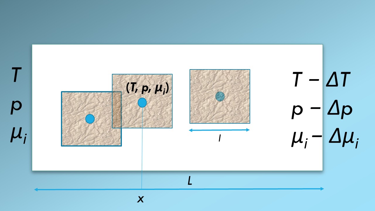
Figure 1: Schematic illustration of a heterogeneous system (white box, length $L$) exposed to a difference in temperature, $\Delta T$, pressure, $\Delta p$ or chemical potential $\Delta\mu_{i}$. The system is isolated in the $y,z-$directions. Net flows take place in the $x-$direction. Three representative elementary volumes, REVs (magenta squares, length $l$) are indicated. The REVs may overlap. Each is represented by a set of variables $(p,T,\mu_{i})$ which defines a state (blue dot). Such states can be defined anywhere on the $x$-axis.

The system is a porous medium of fixed porosity filled with several immiscible fluids. There is net transport in one direction only, the $x$-direction. On the scale of measurement, the system is without structure. By zooming in, we see the pore scale. A collection of pores with two fluids is schematically shown in Figure 2.

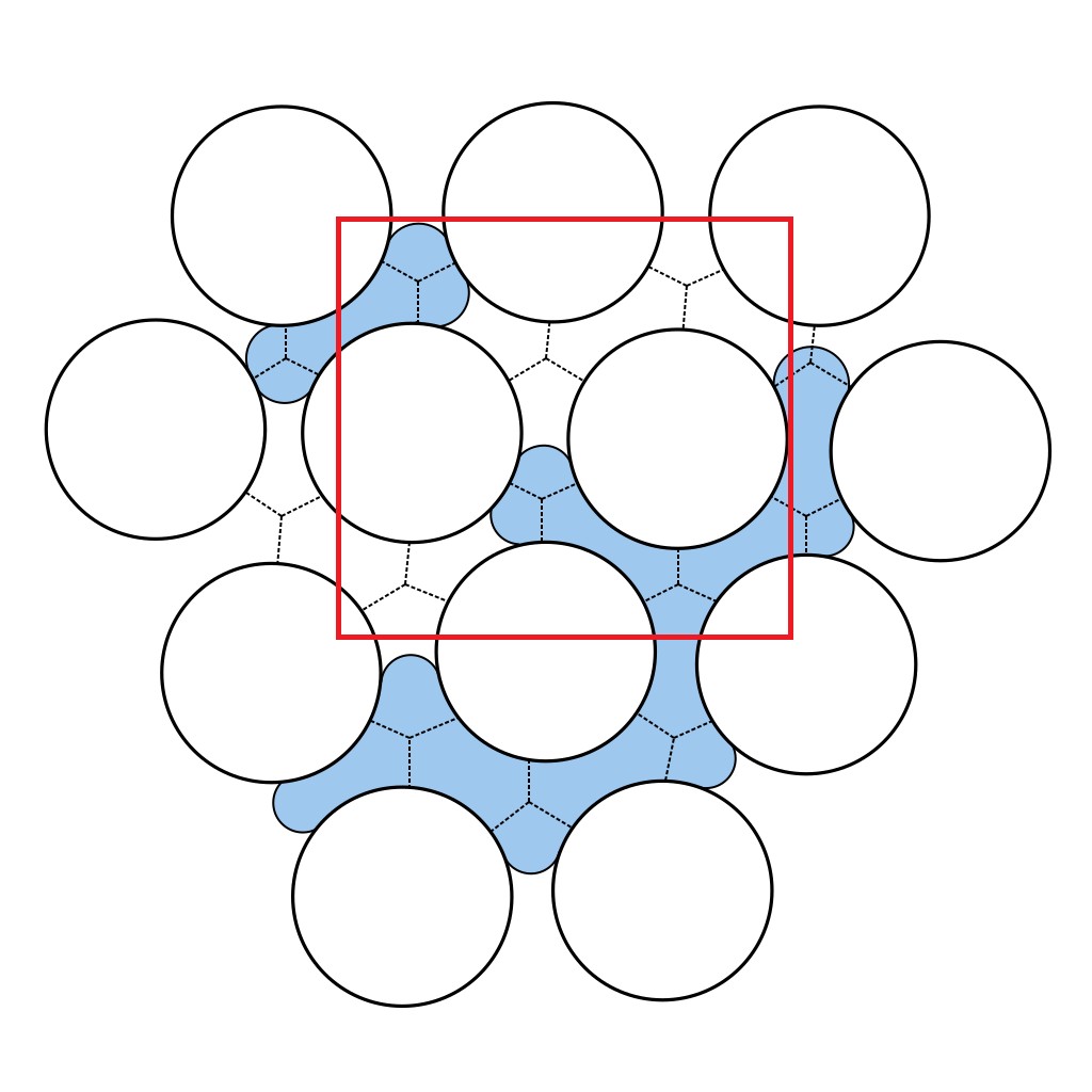
Figure 2: A collection of pores filled with two immiscible liquids. In order to compute the system properties, we define a REV. A REV is indicated in the figure by the red square. Courtesy of M. Vassvik

A temperature, pressure or chemical potential difference is applied between the inlet and the outlet, and these differences can be measured. The pressure difference $\Delta p$ between the outlet and the inlet was defined for steady state conditions by Tallakstad et al. [15], as the time average of the fluctuating difference $\Delta p(t)$:

$$\Delta p=\frac{1}{t_{\mathrm{e}}-t_{\mathrm{b}}}\int_{t_{\mathrm{b}}}^{t_{\mathrm{e}}}\Delta p(t)dt.$$ (1)

Here $t$ is the time. Subscript ’b’ denotes beginning and ’e’ denotes the end of the measurement. We adopt similar definitions for $\Delta T$ and $\Delta\mu_{i}$. It is possible, through application of separate inlet channels, to control the flow into and out of the system and find the flow of each component, to define the flow situation in Fig. 1. In the presence of two immiscible phases, it is only possible to define the pressure difference between the inlet and the outlet for the phases, $\Delta p^{w}$ and $\Delta p^{n}$, if there is continuity in the respective phases.

We will repeatedly use two-phase flow as example, where $w$ indicates the most wetting and $n$ the least wetting phase. We refer to them simply as the wetting and the non-wetting phase. In most of the paper we consider a multi-phase fluid. In the system pictured in Fig. 2, there is flow within the REV in the direction of the pore, which we will also call a link. This is not necessarily the direction given by the overall pressure gradient. The flow on the macro-scale, however, is always in the direction of the pressure gradient. Net flow in other directions are zero due to isolation of the system in these directions. By flow on the macro-scale, we mean flow in the direction of the overall pressure gradient along the $x$-coordinate in Fig.1. The value of this average flow is of interest.

The representative volume element, REV, is constructed from a collection of pores like those contained in the red square in Fig.2. In Fig.1, three REVs are indicated (magenta structured squares). In a homogeneous system, statistical mechanical distributions of molecular properties lead to the macroscopic properties of a volume element. In a heterogeneous system like here, the statistical distributions are over the states within the REV. The collection of pores in the REV, cf. Fig. 2, should be of a size that is large enough to provide meaningful values for the extensive variables, and therefore well defined intensive variables (see below, Eqs. 18 and 19), cf. section 3.2 below. Thermodynamic relations can be written for each REV.

State variables characterize the REV. They are represented by the (blue) dots in Fig. 1. The size of the REV depends on its composition and other conditions. Typically, the extension of a REV, $l$, is large compared to the pore size of the medium, and small compared to the full system length $L$. This construction of a REV is similar to the procedure followed in smoothed particle hydrodynamics [16], cf. the discussion at the end of the work.

The REVs so constructed, can be used to make a path of states, over which we can integrate across the system. Each REV in the series of states, is characterized by variables $T,p,\mu_{i}$, as indicated by the blue dots in Fig.1. Vice versa, each point in a porous medium can be seen as a center in a REV. The states are difficult to access directly, but can be accessed via systems in equilibrium with the states, as is normal in thermodynamics. This is discussed at the end of the work. We proceed to define the REV-variables.

3 Properties of the REV

3.1 Porosity and saturation

Consider a solid matrix of constant porosity $\phi$. We are dealing with a class of systems that are homogeneous in the sense that the typical pore diameter and pore surface area are, on the average, the same everywhere. The pores are filled with a mixture of $m-1$ fluid phases; the solid matrix is labeled $m$. Properties will depend on the time, but this will not be indicated explicitly in the equations.

The system is filled with $m$ phases. In a simple case, the phases are immiscible, and chemical constituents are synonymous with a phase. The state of the REV can be characterized by the volumes of the fluid phases $V^{\alpha,\mathrm{REV}}$, $\alpha=1,..,m-1$ and of the solid medium $V^{m,\mathrm{REV}}$. The total volume of the pores is

$$V^{p,\text{REV}}\equiv\sum_{\alpha=1}^{m-1}V^{\alpha,\text{REV}}.$$ (2)

while the volume of the REV is

$$V^{\text{REV}}\equiv V^{m,\mathrm{REV}}+V^{p,\text{REV}}+\sum_{\alpha>\beta>\delta=1}^{m}V^{\alpha\beta\delta,\text{REV}}.$$ (3)

Superscript REV is used to indicate a property of the REV. The last term is the sum of the excess volumes of the three-phase contact lines. While the excess volume of the surfaces is zero by definition, this is not the case for the three-phase contact lines. The reason is that the dividing surfaces may cross each other at three lines which have a slightly different location. The corresponding excess volume is in general very small, and will from now on be neglected. This gives the simpler expression

$$V^{\text{REV}}\equiv V^{m,\mathrm{REV}}+V^{p,\text{REV}}.$$ (4)

All these volumes can be measured.

The porosity, $\phi$, and the saturation, $\hat{S}$, are given by

$$\phi\equiv\frac{V^{p,\text{REV}}}{V^{\text{REV}}}\ \ \ \ \ \mathrm{{and}\ \ }\hat{S}^{\alpha}\equiv\frac{V^{\alpha,\text{REV}}}{V^{p,\text{REV}}}=\frac{V^{\alpha,\text{REV}}}{\phi V^{\text{REV}}}.$$ (5)

The porosity and the saturation are intensive variables. They do not depend on the size of the REV. They have therefore no superscript. It follows from these definitions that

$$\sum_{\alpha=1}^{m-1}\hat{S}^{\alpha}=1\ \ \ \ \ \mathrm{{and}\ \ }V^{m,\text{REV}}=\left(1-\phi\right)V^{\text{REV}}$$ (6)

In addition to the volumes of the different bulk phases (they are fluids or solids) $m\geq\alpha\geq 1$, there are interfacial areas, $\Omega$, between each two phases in the REV: $\Omega^{\alpha\beta\text{,REV}},\ m\geq\alpha>\beta\geq 1$. The total surface area of the pores is measurable. It can be split between various contributions

$$\Omega^{p\text{,REV}}=\sum_{\alpha=1}^{m-1}\Omega^{m\alpha\text{,REV}}$$ (7)

When the surface is not completely wetted, we can estimate the surface area between the solid $m$ and the fluid phase $\alpha$, from the total pore area available and the saturation of the component.

$$\Omega^{m\alpha\text{,REV}}=\hat{S}^{\alpha}\Omega^{p\text{,REV}}$$ (8)

This estimate is not correct for strongly wetting components or dispersions. In those cases, films can be formed at the walls, and $\Omega^{m\alpha\text{,REV}}$ is not proportional to $\hat{S}^{\alpha}$. In the class of systems we consider, all fluids touch the wall, and there are no films of one fluid between the wall and another fluid.

3.2 Thermodynamic properties of the REV

We proceed to define the thermodynamic properties of the REV within the volume $V^{\mathrm{REV}}$ described above. In addition to the volume, there are other additive variables. They are the masses, the energy and the entropy. We label the components (the chemical constituents) using italic subscripts. There are in total $n$ components distributed over the phases, surfaces and contact lines. The mass of component $i$, $M_{i}^{\text{REV}}$, in the REV is the sum of bulk masses, $M_{i}^{\alpha,\text{REV}}$, $m\geq\alpha\geq 1$, the excess interfacial masses, $M_{i}^{\alpha\beta,\text{REV}}$, $m\geq\alpha>\beta\geq 1$, and the excess line masses, $M_{i}^{\alpha\beta\delta,\text{REV}}$, $m\geq\alpha>\beta>\delta\geq 1$.

$$M_{i}^{\text{REV}}=\sum_{\alpha=1}^{m}M_{i}^{\alpha,\text{REV}}+\sum_{\alpha>\beta=1}^{m}M_{i}^{\alpha\beta,\text{REV}}+\sum_{\alpha>\beta>\delta=1}^{m}M_{i}^{\alpha\beta\delta,\text{REV}}$$ (9)

There is some freedom in how we allocate the mass to the various phases and interfaces [17, 9]. We are e.g. free to choose a dividing surface such that one $M_{i}^{\alpha\beta,\text{REV}}$ equals zero. A zero excess mass will simplify the description, but will introduce a reference. The dividing surface with zero $M_{i}^{\alpha\beta,\text{REV}}$ is the equimolar surface of component $i$. The total mass of a component in the REV is, however, independent of the location of the dividing surfaces. From the masses, we compute the various mass densities

$$\rho_{i} \equiv \frac{M_{i}^{\text{REV}}}{V^{\text{REV}}},\ \ \rho_{i}^{\alpha}\equiv\frac{M_{i}^{\alpha,\text{REV}}}{V^{\alpha,\text{REV}}},\ \$$

$$\rho_{i}^{\alpha\beta} \equiv \frac{M_{i}^{\alpha\beta,\text{REV}}}{\Omega^{\alpha\beta,\text{REV}}},\ \ \rho_{i}^{\alpha\beta\delta}\equiv\frac{M_{i}^{\alpha\beta\delta,\text{REV}}}{\Lambda^{\alpha\beta\delta,\text{REV}}}$$ (10)

where $\rho_{i}$ and $\rho_{i}^{\alpha}$ have dimension kg.m^-3, $\rho_{i}^{\alpha\beta}$ has dimension kg.m^-2 and $\rho_{i}^{\alpha\beta\delta}$ has dimension kg.m^-1.

All densities are for the REV. If we increase the size of the REV, by for instance doubling its size, $V^{\text{REV}}$, $M_{i}^{\text{REV}}$ and other extensive variables will all double. They will double, by doubling all contributions to these quantities. But this is not the case for the density $\rho_{i}$ or the other densities. They remain the same, independent of the size of the REV. This is true also for the densities of the bulk phases, surfaces and contact lines. Superscript REV is therefore not used for the densities.

Within one REV there are natural fluctuations in the densities. But the densities make it possible to give a description on the macro-scale independent of the precise size of the REV. The densities will thus be used in our description on the macro-scale. The density $\rho_{i}^{\alpha}$ may vary somewhat in $V^{\alpha}$. We can then find $M_{i}^{\alpha}$ as the integral of $\rho_{i}^{\alpha}$ over $V^{\alpha}$. Equation 10 then gives the volume-averaged densities.

The internal energy of the REV, $U^{\text{REV}}$, is the sum of bulk internal energies, $U^{\alpha,\text{REV}}$, $m\geq\alpha\geq 1$, the excess interfacial internal energies, $U^{\alpha\beta,\text{REV}}$, $m\geq\alpha>\beta\geq 1$, and the excess line internal energies, $U^{\alpha\beta\delta,\text{REV}}$, $m\geq\alpha>\beta>\delta\geq 1$:

$$U^{\text{REV}}=\sum_{\alpha=1}^{m}U^{\alpha,\text{REV}}+\sum_{\alpha>\beta=1}^{m}U^{\alpha\beta,\text{REV}}+\sum_{\alpha>\beta>\delta=1}^{m}U^{\alpha\beta\delta,\text{REV}}$$ (11)

The summation is taken over all phases, interfaces and contact lines (if non-negligible). We shall see in a subsequent paper how these contributions may give specific contributions to the driving force. The internal energy densities are defined by

$$u \equiv \frac{U^{\text{REV}}}{V^{\text{REV}}},\ \ u^{\alpha}\equiv\frac{U^{\alpha,\text{REV}}}{V^{\alpha,\text{REV}}},\ \$$

$$u^{\alpha\beta} \equiv \frac{U^{\alpha\beta,\text{REV}}}{\Omega^{\alpha\beta,\text{REV}}},\ \ u^{\alpha\beta\delta}\equiv\frac{U^{\alpha\beta\delta,\text{REV}}}{\Lambda^{\alpha\beta\delta,\text{REV}}}$$ (12)

Their dimensions are J.m^-3 ($u,u^{\alpha}$), J.m^-2 ($u^{\alpha\beta}$) and J.m^-1 ($u^{\alpha\beta\delta}$), respectively.

The entropy in the REV, $S^{\text{REV}}$, is the sum of bulk entropies, $S^{\alpha,\text{REV}}$, $m\geq\alpha\geq 1$, the excess entropies, $S^{\alpha\beta,\text{REV}}$, $m\geq\alpha>\beta\geq 1$, and the excess line entropies, $S^{\alpha\beta\delta,\text{REV}}$, $m\geq\alpha>\beta>\delta\geq 1$:

$$S^{\text{REV}}=\sum_{\alpha=1}^{m}S^{\alpha,\text{REV}}+\sum_{\alpha>\beta=1}^{m}S^{\alpha\beta,\text{REV}}+\sum_{\alpha>\beta>\delta=1}^{m}S^{\alpha\beta\delta,\text{REV}}$$ (13)

The entropy densities are defined by

$$s\equiv\frac{S^{\text{REV}}}{V^{\text{REV}}},\ \ s^{\alpha}\equiv\frac{S^{\alpha,\text{REV}}}{V^{\alpha,\text{REV}}},\ \ s^{\alpha\beta}\equiv\frac{S^{\alpha\beta,\text{REV}}}{\Omega^{\alpha\beta,\text{REV}}},\ \ s^{\alpha\beta\delta}\equiv\frac{S^{\alpha\beta\delta,\text{REV}}}{\Lambda^{\alpha\beta\delta,\text{REV}}}$$ (14)

and have the dimensions J.K^-1.m^-3 ($s,s^{\alpha}$), J.K^-1.m^-2 ($s^{\alpha\beta}$) and J.K^-1.m^-1 ($s^{\alpha\beta\delta}$), respectively. The entropy will in addition have a configurational contribution from the mixture of components (phases) when there is a distribution of states within the heterogeneous mixture. To explain this in more detail; consider the example of the entropy of a two-phase fluid in a long, narrow tube of variable diameter. None of the fluids are forming films between the tube walls and the other fluid, and the long tube can be regarded as an ensemble of shorter tubes, each containing a bubble [18]. The configurational term can then be given in terms of the probability to find the position of a bubble at position $x_{b}$.

For the volume, Eqs.2 and 4 apply when the contact lines give a negligible contribution. The dividing surfaces by definition have no excess volume. For all the other extensive thermodynamic variables, like the enthalpy, Helmholtz, Gibbs energies and the grand potential, relations similar to Eq.11 and 13 apply.

To summarize this section; we have defined a basis set of variables for a class of systems, where these variables are additive in the manner shown. From the set of REV variables we obtain the densities, $u$, $s$ or $\rho_{i}$ to describe the heterogeneous system on the macro-scale. A series of the REVs of this type, is needed for integration across the system, see section 5.

The surface areas and the contact line lengths are not independent variables in this representation of the REV. These variables are, however, included indirectly through the assumption that the basic variables of the REV are additive. This means that a REV of a double size has double the energy, entropy, and mass, but also double the surface areas of various types and double the line lengths.

3.3 REV size considerations

As an illustration of the REV construction, consider the internal energy of two isothermal, immiscible and incompressible fluids (water and decane) flowing in a Hele-Shaw cell composed of silicone glass beads. The relevant properties of the fluids can be found in Table 1. The porous medium is a hexagonal network of 3600 links, as illustrated in Figure 3. The network is periodic in the longitudinal and the transverse directions and a pressure difference of 1.8 $\times$ 10⁴ Pa drives the flow in the longitudinal direction. The overall saturation of the water is 0.4. The network flows were simulated using the method of Aker et al. [19], see Ref. [20] for details.

The internal energy of the REV is, according to Section 3.2, a sum over the two fluid bulk contributions and three interface contributions,

$$U^{\text{REV}} =U^{m,\text{REV}}+\sum_{i\in\left\{w,n\right\}}\left\{U^{i,\text{REV}}\right\}+U^{wn,\text{REV}}+U^{np,\text{REV}}+U^{wp,\text{REV}}$$ (15)

$$=U^{m,\text{REV}}+V^{p,\text{REV}}\sum_{i\in\left\{w,n\right\}}\left\{\hat{S}^{i}u^{i}\right\}+u^{wn}\Omega^{wn,\text{REV}}+u^{np}\Omega^{np,\text{REV}}+u^{wp}\Omega^{wp,\text{REV}}.$$ (16)

where, $u^{i}$ is the internal energy density of phase $i$ and $u^{ij}$ is the excess internal energy per interfacial area between phase $i$ and phase $j$. We assume $u^{i}$ and $u^{ij}$ to be constant. For simplicity, $u^{ij}$ is approximated by interfacial tension, denoted $\gamma^{ij}$. The internal energy of the porous matrix is constant in this example and is therefore set to zero.

Table 1: Fluid properties used to compute the candidate REV internal energy, for a network containing water (n) and decane (w) within silicone glass (p) at atmospheric pressure and 293 K.

Parameter	Value	Unit	Reference
$\eta^{w}$	9.2 $\times$ 10-4	Pa.s	[21]
$\eta^{n}$	1.0 $\times$ 10-3	Pa.s	[21]
$\gamma^{wp}$	2.4 $\times$ 10-2	N.m-1	[22]
$\gamma^{np}$	7.3 $\times$ 10-2	N.m-1	[22]
$\gamma^{wn}$	5.2 $\times$ 10-2	N.m-1	[23]
$-u^{w}$	2.8 $\times$ 108	J.m-3	[21]
$-u^{n}$	3.4 $\times$ 108	J.m-3	[21]

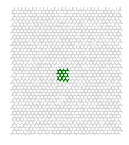
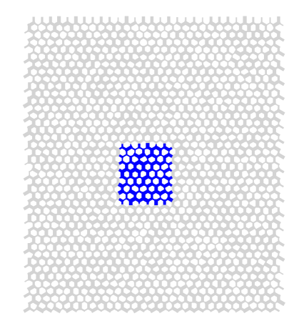
Figure 3: Illustration of the link network and two of the candidate REVs under consideration. The left candidate REV (green) is 5.2mm $\times$ 6mm and the right candidate REV (blue) is 10.4mm$\times$ 12mm.

Candidate REVs are of different sizes, see Table 2. The 5.4 mm $\times$ 6 mm (green), and 10.4 mm $\times$ 12 mm (blue) candidate REVs are shown in Figure 3. For all candidate REVs, $U^{\text{REV}}$ is calculated according to Eq. 16 at each time step. Since the measured saturations and interfacial areas are fluctuating in time, so is the internal energy. A time-step weighted histogram of the internal energy presents the probability distribution.

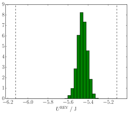
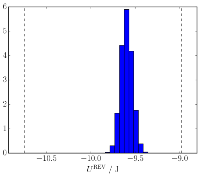
Figure 4: Probability distributions of internal energy in two the candidate REVs. The left candidate REV (green) is 5.2mm $\times{6}$ mm and the right candidate REV (blue) is 10.4 mm$\times{12}$ mm. In each plot, the left dashed line represents the internal energy the candidate REV would have if it contained non-wetting fluid only and the right dashed line represents the internal energy the candidate REV would have if it contained wetting fluid only.

The probability distributions of $U^{\text{REV}}$ are shown in Figure 4 for the 5.2 mm $\times$ 6 mm (green) and 10.4 mm $\times$ 12 mm (blue) candidate REVs. In both plots, the vertical lines represent the internal energy the REV would have if it were occupied by one of the fluids alone. We denote the difference in internal energy between these two single-phase states by $\Delta U^{\text{REV}}$.

Table 2: Mean values of $U^{\text{REV}}$ and $u$ for candidate REVs of different sizes, along with the standard deviation of $U^{\text{REV}}$ divided by $\Delta U^{\text{REV}}$. The latter quantity represents a measure of the relative size of the fluctuations in $U^{\text{REV}}$.

Candidate REV	mean $\left(U^{\text{REV}}\right)$	$\pm\left(U^{\text{REV}}\right)$	mean $\left(u\right)$
Size	/J	/$\Delta U^{\text{REV}}$	/ 107 J m-3
5.2 mm $\times$ 6.0 mm	-2.82	0.069	-6.04
7.8 mm $\times$ 9.0 mm	-5.46	0.047	-5.19
10.4 mm $\times$ 12.0 mm	-9.60	0.037	-5.13
13.0 mm $\times$ 15.0 mm	-15.4	0.028	-5.25
15.6 mm $\times$ 18.0 mm	-22.2	0.024	-5.27
18.3 mm $\times$ 21.0 mm	-29.9	0.021	-5.22
20.8 mm $\times$ 24.0mm	-39.1	0.017	-5.23

The mean value of the $U^{\text{REV}}$ for all candidate REVs are given in Table 2, along with mean density $u=U^{\text{REV}}/V^{\text{REV}}$ and the standard deviation of $U^{\text{REV}}$ divided by $\Delta U^{\text{REV}}$. The latter quantity is a measure of the relative size of the fluctuations in $U^{\text{REV}}$. Due to the additivity of $U^{\text{REV}}$, the mean values of $U^{\text{REV}}$ increases roughly proportional to the candidate REV size. But this happens only after the REV has reached a minimum size, here 7.8 mm $\times$ 9.0 mm. For the larger candidate REVs, the mean value of $u$ changes little as the size increases. The relative size of the fluctuations in $U^{\text{REV}}$ decreases in proportion to the linear size of the candidate REVs.

This example indicates that it makes sense to characterize the internal energy of a porous medium in terms of an internal energy density as defined by Eq. 11, given that the size of the REV is appropriately large. About 100 links seem to be enough in this case. This will vary with the type of porous medium, cf. the 2D square network model of Savani et al. [24].

4 Homogeneity on the macro-scale

Before we address any transport problems, consider again the system pictured in Fig.1 (the white box). All REVs have variables and densities as explained above. By integrating to a somewhat larger volume $V$, using the densities defined, we obtain the set of basis variables, ($U,S,M_{i}$), in $V$. The internal energy $U$ of the system is an Euler homogeneous function of first order in $S,V,M_{i}$:

$$U\left(\lambda S,\lambda V,\lambda M_{i}\right)=\lambda U\left(S,V,M_{i}\right)$$ (17)

The internal energy $U,$ volume $V$, entropy $S$, and component mass $M_{i}$, obey therefore the Gibbs equation;

$$dU=\left(\frac{\partial U}{\partial S}\right)_{V,M_{i}}dS+\left(\frac{\partial U}{\partial V}\right)_{S,M_{i}}dV+\sum_{i=1}^{n}\left(\frac{\partial U}{\partial M_{i}}\right)_{S,V,M_{j}}dM_{i}$$ (18)

No special notation is used here to indicate that $U,S,V,M_{i}$ are properties on the macro-scale. Given the heterogeneous nature on the micro-scale, the internal energy has contributions from all parts of the volume $V$, including from the excess surface and line energies. By writing Eq.17 we find that the normal thermodynamic relations apply for the heterogeneous system at equilibrium, additive properties $U,S,V,M_{i}$, obtained from sums of the bulk-, excess surface- and excess line-contributions.

We can then move one more step and use Gibbs equation to define the temperature, the pressure and chemical potentials on the macro-scale as partial derivatives of $U$:

$$T\equiv\left(\frac{\partial U}{\partial S}\right)_{V,M_{i}},\ \ p\equiv-\left(\frac{\partial U}{\partial V}\right)_{S,M_{i}},\ \ \mu_{i}\equiv\left(\frac{\partial U}{\partial M_{i}}\right)_{S,V,M_{j}}$$ (19)

The temperature, pressure and chemical potentials on the macro-scale are, with these formulas, defined as partial derivatives of the internal energy. This is normal in thermodynamics, but the meaning is now extended. In a normal homogeneous, isotropic system at equilibrium, the temperature, pressure and chemical equilibrium refer to a homogeneous volume element. The temperature of the REV is a temperature representing all phases, interfaces and lines combined, and the chemical potential of $i$ is similarly obtained from the internal energy of all phases. Therefore, there are only one $T,p$ and $\mu_{i}$ for the REV. The state can be represented by the (blue) dots in Fig.1.

On the single pore level, the pressure and temperature in the REV will have a distribution. In the two immiscible-fluid-example the pressure, for instance, will vary between a wetting and a non-wetting phase because of the capillary pressure. One may also envision that small phase changes in one component (e.g. water) leads to temperature variations due to condensation or evaporation. Variations in temperature will follow changes in composition.

The intensive properties are not averages of the corresponding entities on the pore-scale over the REV. This was pointed out already by Gray and Hassanizadeh [3]. The definitions are derived from the total internal energy only, and this makes them uniquely defined. It is interesting that the intensive variables do not depend on how we split the energy into into bulk and surface terms inside the REV.

By substituting Eq.19 into Eq.18 we obtain the Gibbs equation for a change in total internal energy on the macro-scale

$$dU=TdS-pdV+\sum_{i=1}^{n}\mu_{i}dM_{i}$$ (20)

As a consequence of the condition of homogeneity of the first order, we also have

$$U=TS-pV+\sum_{i=1}^{n}\mu_{i}M_{i}$$ (21)

The partial derivatives $T,\ p$ and $\mu_{i}$ are homogeneous functions of the zeroth order. This implies that

$$T(\lambda S,\lambda V,\lambda M_{i})=T(S,V,M_{i})$$ (22)

Choosing $\lambda=1/V$ it follows that

$$T(S,V,M_{i})=T(s,1,\rho_{i})=T(s,\rho_{i})$$ (23)

The temperature therefore depends only on the subset of variables $s\equiv S/V,\rho_{i}\equiv M_{i}/V$ and not on the complete set of variables $S,V,M_{i}$. The same is true for the pressure, $p$, and the chemical potentials, $\mu_{i}$. This implies that $T,\ p$ and $\mu_{i}$ are not independent. We proceed to repeat the standard derivation of the Gibbs-Duhem equation which makes their interdependency explicit.

The Gibbs equation on the macro-scale in terms of the densities follows using Eqs. 20 and 21

$$du=Tds+\sum_{i=1}^{n}\mu_{i}d\rho_{i}$$ (24)

which can alternatively be written as

$$ds=\frac{1}{T}du-\frac{1}{T}\sum_{i=1}^{n}\mu_{i}d\rho_{i}$$ (25)

The Euler equation implies

$$u=Ts-p+\sum_{i=1}^{n}\mu_{i}\rho_{i}$$ (26)

By differentiating Eq. (26) and subtracting the Gibbs equation (24), we obtain in the usual way the Gibbs-Duhem equation:

$$dp=sdT+\sum_{i=1}^{n}\rho_{i}d\mu_{i}$$

This equation makes it possible to calculate $p$ as a function of $T$ and $\mu_{i}$ and shows how these quantities depend on one another.

We have now described the heterogeneous porous medium by a limited set of coarse-grained thermodynamic variables. These average variables and their corresponding temperature, pressure and chemical potentials, describe a coarse-grained homogeneous mixture with variables which reflect the properties of the class of porous media. In standard equilibrium thermodynamics, Gibbs’ equation applies to a homogeneous phase. We have extended this use to be applicable for heterogeneous systems at the macro-scale. Whether or not the chosen procedure is viable, remains to be tested. We refer to the Section 7 of this paper.

5 Entropy production in porous media

Gradients in mass- and energy densities produce changes in the variables on the macro-scale. These lead to transport of heat and mass. Our aim is to find the equations that govern this transport across the REV. We therefore expose the system to driving forces and return to Fig. 1.

The balance equations for masses and internal energy of a REV are

$$\frac{\partial\rho_{i}}{\partial t} = -\frac{\partial}{\partial x}J_{i}$$ (27)

$$\frac{\partial u}{\partial t} = -\frac{\partial}{\partial x}J_{u}=-\frac{\partial}{\partial x}\left[J_{q}^{{}^{\prime}}+\sum_{i=1}^{n}J_{i}H_{i}\right]$$ (28)

The transport on this scale is in the $x-$direction only. The mass fluxes, $J_{i}$, and the flux of internal energy, $J_{u}$, are all macro-scale fluxes. The internal energy flux is the sum of the measurable (or sensible) heat flux, $J_{q}^{{}^{\prime}}$ and the partial specific enthalpy (latent heat), $H_{i}$ (in J.kg^-1) times the component fluxes, $J_{i}$, see [7, 3, 9] for further explanations. Component $m$ (the porous medium) is not moving and is the convenient frame of reference for the fluxes.

The entropy balance on the macro-scale is

$$\frac{\partial s}{\partial t}=-\frac{\partial}{\partial x}J_{s}+\sigma$$ (29)

Here $J_{s}$ is the entropy flux, and $\sigma$ is the entropy production which is positive definite, $\sigma\geq 0$ (the second law of thermodynamics). We can now derive the expression for $\sigma$ in the standard way [7, 9], by combining the balance equations with Gibbs’ equation. The entropy production is the sum of all contributions within the REV.

In the derivations, we assume that the Gibbs equation is valid for the REV also when transport takes place. Droplets can form at high flow rates, while ganglia may occur at low rates. We have seen above that there is a minimum size of the REV, for which the Gibbs equation can be written. When we assume that the Gibbs equation applies, we implicitly assume that there exists a uniquely defined state. The existence of such a state was first postulated by Hansen and Ramstad [25]. Experimental evidence for the assumption was found by Erpelding [26].

Under the conditions we demand for the REV, the Gibbs equation Eq.25 keeps its form during a time interval $dt$, giving

$$\frac{\partial s}{\partial t}=\frac{1}{T}\frac{\partial u}{\partial t}-\frac{1}{T}\sum_{i=1}^{n}\mu_{i}\frac{\partial\rho_{i}}{\partial t}$$ (30)

We can now introduce the balance equations for mass and energy into this equation, see [9] for details. By comparing the result with the entropy balance, Eq.29, we identify first the entropy flux, $J_{s}$,

$$J_{s}=\frac{1}{T}J_{q}^{\prime}+\sum_{i=1}^{n}J_{i}S_{i}$$ (31)

The entropy flux is composed of the sensible heat flux over the temperature plus the sum of the specific entropies carried by the components. The form of the entropy production, $\sigma$, depends on our choice of the energy flux, $J_{u}$ or $J_{q}^{\prime}$. The choice of form is normally motivated by practical wishes; what is measurable or computable. We have

$$\sigma = J_{u}\frac{\partial}{\partial x}(\frac{1}{T})-\sum_{i=1}^{n}J_{i}\frac{\partial}{\partial x}(\frac{\mu_{i}}{T})$$ (32)

$$= J_{q}^{\prime}\frac{\partial}{\partial x}(\frac{1}{T})-\frac{1}{T}\sum_{i=1}^{n}J_{i}\frac{\partial}{\partial x}\mu_{i,T}$$

These expressions are equivalent formulations of the same physical phenomena. When we choose $J_{u}$ as variable with the conjugate force $\partial(1/T)/\partial x$, the mass fluxes are driven by minus the gradient in the Planck potential ${\mu_{i}}/{T}$. When, on the other hand we choose $J_{q}^{\prime}$ as a variable with the conjugate force $\partial(1/T)/\partial x$, the mass fluxes are driven by minus the gradient in the chemical potential at constant temperature over this temperature. The entropy production defines the independent thermodynamic driving forces and their conjugate fluxes. We have given two possible choices above to demonstrate the flexibility. The last expression is preferred for analysis of experiments.

In order to find the last line in Eq.32 from the first, we used the thermodynamic identities $\mu_{i}=H_{i}-TS_{i}$ and $\partial(\mu_{i}/T)/\partial(1/T)=H_{i}$ as well as the expression for the energy flux given in Eq.28. Here $S_{i}$ is the partial specific entropy (in J.kg^-1.K^-1).

5.1 The chemical potential at constant temperature

The derivative of the chemical potential at constant temperature is needed in the driving forces in the second line for $\sigma$ in Eq.32. For convenience we repeat its relation to the full chemical potential [7]. The differential of the full chemical potential is:

$$d\mu_{i}=-S_{i}dT+V_{i}dp+\sum_{j=1}^{n}\left(\frac{\partial\mu_{i}}{\partial M_{j}}\right)_{p,T,M_{i}}dM_{j}$$ (33)

where $S_{i},V_{i}$ and $({\partial\mu_{i}}/{\partial M_{j}})_{p,T,M_{i}}$ are partial specific quantities. The partial specific entropy and volume are equal to:

$$S_{i}=-\left(\frac{\partial\mu_{i}}{\partial T}\right)_{p,M_{j}}\ ,\ V_{i}=\left(\frac{\partial\mu_{i}}{\partial p}\right)_{T,M_{j}}$$ (34)

and the last term of Eq. 32 is denoted by

$$d\mu_{i}^{c}=\sum_{j=1}^{n}\left(\frac{{\partial\mu_{i}}}{{\partial M_{j}}}\right)_{p,T,M_{i}}dM_{j}$$ (35)

By reshuffling, we have the quantity of interest as the differential of the full chemical potential plus an entropic term;

$$d\mu_{i,T}\equiv d\mu_{i}+S_{i}dT=V_{i}dp+d\mu_{i}^{c}$$ (36)

The differential of the chemical potential at constant temperature is

$$\frac{d\mu_{i,T}}{dx}=\frac{d\mu_{i}^{c}}{dx}+V_{i}\frac{dp}{dx}$$ (37)

With equilibrium in the gravitational field, the pressure gradient is $dp/dx=-\rho g$, where $\rho$ is the total mass density and $g$ is the acceleration of free fall [27]. The well known separation of components in the gravitational field is obtained, with $d\mu_{i,T}=0$ and

$$\frac{d\mu_{i}^{c}}{dx}=\frac{RT}{W_{i}}\frac{d\ln(\hat{S}_{i}y_{i})}{dx}=V_{i}\rho g$$ (38)

where $W_{i}$ is the molar mass (in kg.mol^-1), $\hat{S}_{i}$ the saturation, and $y_{i}$ the activity coefficient of component $i$. The gas constant, $R$, has dimension J.K${}^{-1}.$mol^-1. The gradient of the mole fraction of methane and decane in the geothermal gradient of the fractured carbonaceous Ekofisk oil field, was estimated to 5x10^-4m^-1 [28], in qualitative agreement with observations. We replace $d\mu_{i,T}$ below using these expressions.

It follows from Euler homogeneity that the chemical potentials in a (quasi-homogeneous) mixture are related by $0=SdT-Vdp+\sum_{j=1}^{n}\rho_{j}d\mu_{j}$, which is Gibbs-Duhem’s equation. By introducing 36 into this equation we obtain an equivalent expression, to be used below:

$$0=\sum_{j=1}^{n}\rho_{j}d\mu_{j}^{c}$$ (39)

6 Transport of heat and two-phase fluids

Consider again the case of two immiscible fluids, one more wetting (w) and one more non-wetting (n). The entropy production in Eq.32 gives,

$$\sigma=J_{q}^{\prime}\frac{\partial}{\partial x}(\frac{1}{T})-\frac{1}{T}\left(J_{w}\frac{\partial\mu_{w,T}}{\partial x}+J_{n}\frac{\partial\mu_{n,T}}{\partial x}\right)$$ (40)

The solid matrix is the frame of reference for transport, $J_{r}=0$ and does not contribute to the entropy production. The volume flux is frequently measured, and we wish to introduce this as new variable

$$J_{V}=J_{n}V_{n}+J_{w}V_{w}$$ (41)

Here $J_{V}$ has dimension (m³.m${}^{-2}.$s^-1 = m.s^-1), and the partial specific volumes have dimension m³.kg^-1. The chemical potential of the solid matrix may not vary much if the composition of the solid is constant across the system. We assume that this is the case ($d\mu_{m}^{c}\approx 0$), and use Eq.39 to obtain

$$0=\rho_{n}d\mu_{n}^{c}+\rho_{w}d\mu_{w}^{c}$$ (42)

The entropy production is invariant to the choice of variables. We can introduce the relations above and the explicit expression for $d\mu_{i,T}$ into Eq.40, and find the practical expression:

$$\sigma=J_{q}^{\prime}\frac{\partial}{\partial x}\left(\frac{1}{T}\right)-J_{V}\frac{1}{T}\frac{\partial p}{\partial x}-J_{D}\frac{\rho_{w}}{T}\frac{\partial\mu_{w}^{c}}{\partial x}$$ (43)

In the last line, the difference velocity $J_{D}$ is

$$J_{D}=\frac{J_{w}}{\rho_{w}}-\frac{J_{n}}{\rho_{n}}$$ (44)

This velocity describes the relative movement of the two components within the porous matrix. In other words, it describes the ability of the medium to separate components. The main driving force for separation is the chemical driving force, related to the gradient of the saturation. The equation implies that also temperature and pressure gradients may play a role for the separation.

The entropy production has again three terms, one for each independent driving force. With a single fluid, the number of terms are two. The force conjugate to the heat flux is again the gradient of the inverse temperature. The entropy production, in the form we can obtain, Eqs.40 or 43, dictates the constitutive equations of the system.

The volume flows used by Hansen et al [14] are related to ours by $J_{n}V_{n}=Q_{n}/A^{p}$ and $J_{w}V_{w}=Q_{w}/A^{p}$, where $A^{p}\equiv V^{p}/\ell$ is the cross-sectional area of the pores in the volume normal to the flow direction, and $\ell$ is the length of the volume in the flow direction. In [14] the total volume flow was assumed to be an Euler homogeneous functions of the first order of the fractional areas, $A^{n}\equiv V^{n}/\ell$ and $A^{w}\equiv V^{w}/\ell$ for the two components, respectively. The seepage velocities are $v_{n}=Q_{n}/A^{n}$ and $v_{w}=Q_{w}/A^{w}$. By introducing these variables in the expression for the entropy production, we obtain two alternative forms for the entropy production, Eq. 43:

$$\sigma=J_{q}^{\prime}\frac{\partial}{\partial x}\left(\frac{1}{T}\right)-\frac{1}{A^{p}T}\left[(Q_{w}+Q_{n})\frac{\partial p}{\partial x}+(\frac{Q_{w}}{\rho_{w}V_{w}}-\frac{Q_{n}}{\rho_{n}V_{n}})\rho_{w}\frac{\partial\mu_{w}^{c}}{\partial x}\right]$$ (45)

$$= J_{q}^{\prime}\frac{\partial}{\partial x}\left(\frac{1}{T}\right)-\frac{1}{T}\left[v_{w}\hat{S}_{w}\left(\frac{\partial p}{\partial x}+\frac{1}{V_{w}}\frac{\partial\mu_{w}^{c}}{\partial x}\right)+v_{n}\hat{S}_{n}\left(\frac{\partial p}{\partial x}+\frac{1}{V_{n}}\frac{\partial\mu_{n}^{c}}{\partial x}\right)\right]$$ (46)

In the second identity we used Gibbs-Duhem, Eq. 42. If we define

$$\frac{\partial p_{i}}{\partial x}\equiv\hat{S}_{i}\left(\frac{\partial p}{\partial x}+\frac{1}{V_{i}}\frac{\partial\mu_{i}^{c}}{\partial x}\right)\text{ \ \ for \ }i=n,w$$ (47)

the entropy production can be written as

$$\sigma=J_{q}^{\prime}\frac{\partial}{\partial x}\left(\frac{1}{T}\right)-\frac{1}{T}v_{w}\frac{\partial p_{w}}{\partial x}-\frac{1}{T}v_{n}\frac{\partial p_{n}}{\partial x}$$ (48)

Whether $p_{w}$ and $p_{n}$ have any concrete meaning is not clear. The difference of their gradients is

$$\frac{\partial\left(p_{n}-p_{w}\right)}{\partial x} = \frac{\hat{S}_{n}}{V_{n}}\frac{\partial\mu_{n}^{c}}{\partial x}-\frac{\hat{S}_{w}}{V_{w}}\frac{\partial\mu_{w}^{c}}{\partial x}$$ (49)

$$= \left(\frac{\hat{S}_{n}}{V_{n}\rho_{n}}+\frac{\hat{S}_{w}}{V_{w}\rho_{w}}\right)\rho_{n}\frac{\partial\mu_{n}^{c}}{\partial x}$$

where we again used Gibbs-Duhem in the last identity. As one often identifies the left hand side of this equation with the gradient of the capillary pressure, this would relate this force to the chemical force. We will come back to this issue later.

6.1 A path of sister systems

As pointed out above, through the construction of the REV we were able to create a continuous path through the system, defined by the thermodynamic variables of the REVs. The path was illustrated by a sequence of dots in Fig. 1. Such a path must exist, to make integration possible. Also continuum mixture theory hypothesizes such a path [4]: Hilfer introduced a series of mixture states, to define an integration path across the porous system, see e.g. [4].

The path created in Section 2 is sufficient as a path integration across the medium. The access to and measurement of properties in the REVs is another issue. It is difficult, if not impossible, to measure in situ as stated upfront. The measurement probe has a minimum extension (of some mm), and the measurement will represent an average over the surface of the probe. For a phase with constant density, the average is well defined and measurable. A link between the state of the REV and a state where measurements are possible, is therefore needed. We call the state that provides this link a sister state.

Consider again the path of REVs in the direction of transport. To create the link between the REV and its sister state, consider the system divided into slices, see Figure 5. The slice (the sister system) contains homogeneous phases in equilibrium with the REV at the chosen location.

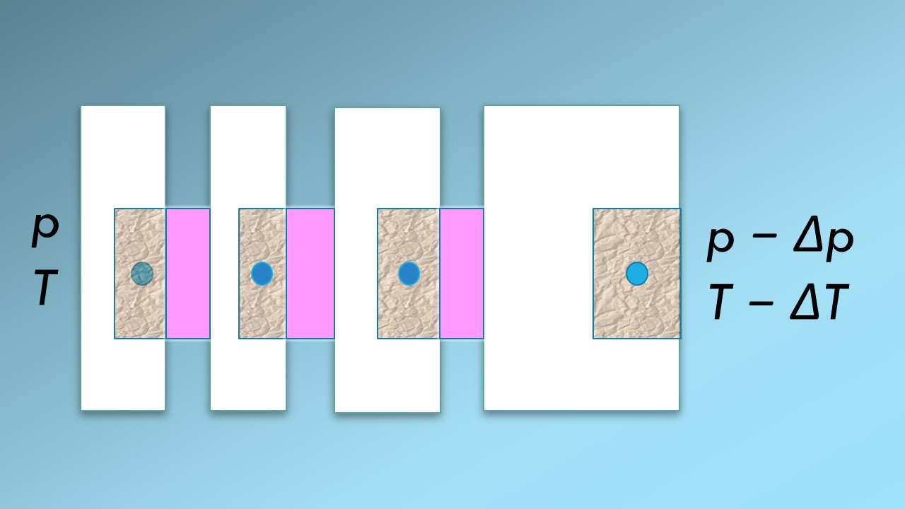
Figure 5: A one-dimensional heterogeneous system cut into slices. Each cut is brought in equilibrium with a homogeneous mixture at the same temperature and pressure as the REV.

We hypothesize that we can find such sister states; in the form of a multi-component mixture with temperature, pressure and composition such that equilibrium can be obtained with for the REV-variables at any slice position. The variables of the sister state can then be measured the normal way. The chemical potential of a component in the sister state can, for instance, be found by introducing a vapor phase above this state and measure the partial vapor pressure. We postulate thus that a sister state can be found, that obey the conditions

$$T = T^{s}$$ (50)

$$p = p^{s}$$ (51)

$$\mu_{i} = \mu_{i}^{s}$$ (52)

Here $i$=1,…n are the components in the REV, and superscript s denotes the sister state. With the sister states available, we obtain an experimental handle on the variables of the porous medium. The hypothesis must be checked, of course.

The series of sister states have the same boundary conditions as the REV-states, by construction, and the overall driving forces will be the same. Between the end states, we envision the non-equilibrium system as a staircase. Each step in the stair made up of REV is in equilibrium with a step of the sister-state-stair. Unlike the states inside the porous medium, the sister states are accessible for measurements, or determination of $T,p$ and $\mu_{i}$. Transport can then be described as taking place along a sequence of the sister states.

7 Discussion

We have seen how we can define a representative elementary volume, called the REV, and conditions such that standard non-equilibrium thermodynamics for homogeneous systems [7] can be extended to describe flow in heterogeneous systems like porous media. The procedure adds a step to earlier elaborations in the field [2, 3]. We have been able to derive the total entropy production directly for the heterogeneous system, and have thus obtained a new basis for constitutive equations of the system on the macro-scale. Earlier, the equation sets were written for the separate parts, or for systems that were homogeneous on the molecular scale [29].

Equations 40 and 43 have been established since long in the theory of transport in polymer membranes, see e.g. [29]. The step to include porous media is inspired by this. The way of dealing with lack of knowledge of variables inside the system was for instance used in polymer membrane transport long ago, see [30, 31]. The procedure, to introduce a series of equilibrium states, each state in equilibrium with the membrane at some location between the external boundaries, was first used by Scatchard [30], and later experimentally verified [31, 32].

The clue to obtain the present results was to use Euler homogeneity on the macro-scale. This allowed us to set up the Gibbs equation with well defined variables, in spite of local variations in, for instance, the pressure inside the REV. Together with the balance equations, this gave the entropy production in a standard way. Some support can be found in the literature. Prigogine and Mazur [33] investigated a mixture of two fluids using non-equilibrium thermodynamics. Their system consisted of superfluid - and normal helium. Two different pressures were defined. For the case they discussed, the interaction between the two fluids was small, meaning that one phase flowed as if the other one (aside from a small frictional force) was not there. The situation here is similar, as we may have different liquid pressures inside the REV. But the interaction between the two immiscible components in our porous medium is large, not negligible as in the helium case.

A central issue in the extension is the construction of the REV. This construction is subject to conservation of the important properties of the system. For instance, the REV must conserve the total porosity of the system. Such constructions are known from other up-scaling techniques. In mesoscale simulations, i.e. upscaling from properties at the nanometer scale to micrometer scale, techniques known as ”Dissipative Particle Dynamcs” stemming from hydrodynamics [34] and ”Smoothed Particle Hydrodynamics”, stemming from astrophysics [16] have been used.

Inspired by the idea behind smoothed particle hydrodynamics, we can also define a normalized weight function $W(\mathbf{r})$, such that a microscopic variable $a(\mathbf{r})$ may be represented by its average, defined as

$$\overline{a}(\mathbf{r})\equiv\int d\mathbf{r}^{\prime}W(\mathbf{r-r}^{\prime})a(\mathbf{r}^{\prime}).$$ (53)

For example, if $a(\mathbf{r}^{\prime})$ is the local void fraction in a porous material as determined from samples of the material, $\overline{a}(\mathbf{r})$ is the average porosity of the medium. The average is assigned to the point $\mathbf{r}$ and varies smoothly in space. The average porosity $\overline{a}(\mathbf{r})$ would then be suitable for e.g. a reservoir simulation at the macro-scale.

In general, the system is subject to external forces and its properties are non-uniform. The choice of $W(\mathbf{r})$ is therefore crucial in that it defines the extent of the coarse-graining and the profile of the weighting. The illustration in Fig. 1 alludes to a weight function that is constant inside a cubic box and zero outside, but other choices are possible. Popular choices used in mesoscale simulations are the Gaussian and spline functions (See [16] for details).

A convenient feature of the coarse-graining is that the average of a gradient of a property $a$ is equal to the gradient of the average.

$$\nabla\overline{a}(\mathbf{r})=\overline{\nabla a(\mathbf{r})}$$ (54)

Similarly the average of a divergence of a flux is equal to the divergence of the average. This implies that balance equations, which usually contain the divergence of a flux, remain valid after averaging.

Time averages can also be introduced along the lines sketched above. Also the average of a time derivative of $a$ becomes equal to the time derivative of the average. Again, the balance equations remain valid after averaging. (In this paper we have not used time averages.) The total amount of $a$ in the volume of the REV is

$$A^{\text{REV}}\equiv\int_{\text{REV}}d\mathbf{r}a(\mathbf{r})\equiv\overline{a}\int_{\text{REV}}d\mathbf{r}\equiv\overline{a}V^{\text{REV}}$$ (55)

The time scale relevant to porous media transport are usually large (minutes, hours); and much larger than times relevant for the molecular scale. Partial derivatives were used in the balance equations and the entropy production. This signifies that properties can change not only along the coordinate axis, but also on the time scale. In the present formulation any change brought about in the REV must retain the validity of the Gibbs equation (i.e. Euler homogeneity). As long as that is true, we may use the equations, also for transient phenomena.

The outcome of the derivations enables us to deal with a wide range of non-isothermal phenomena in a systematic manner, from frost heave to heterogeneous catalysis, or multi-phase flow in porous media. We will elaborate on what this means in the next part of this work. In particular, we shall give more details on the meaning of the additive variables and the REV pressure. We will return to the meaning of the REV variables and how they will contribute to the driving forces of transport.

8 Concluding remarks

We have derived the entropy production for transport of heat and mass in porous media. The derivations have followed standard non-equilibrium thermodynamics for heterogeneous systems [9]. The only, but essential, difference has been the fact that we write all these equations for a porous medium on the macro-scale for the REV of a minimum size using its total entropy, energy and mass, while these equations often are only written for the separate contributions. Broadly speaking, we have been zooming out our view on the porous medium to first define some states that we take as thermodynamic states because they obey Euler homogeneity. The states are those illustrated by the dots in Figure 1. In order to define these states by experiments, we constructed the sister states of Fig.5.

The advantage of the present formulations is this; it is now possible to formulate the transport problem on the scale of a flow experiment in accordance with the second law of thermodynamics, with far less variables. This also opens up the possibility to test the thermodynamic models for use along with and compatibility with this law. Such tests can be explicitly formulated once we have the constitutive equations. In the next part of this work, such details will be given.

We have been dealing as an example with the specific case of immiscible, non-isothermal two-phase flow in a non-deformable medium. In deformable systems, grains may move by translation, compaction and/or rotation. We expect that this situation also can be treated by the procedure given above.

Acknowledgement

The authors are grateful to the Research Council of Norway through its Centres of Excellence funding scheme, project number 262644, PoreLab. Per Arne Slotte is thanked for stimulating discussions.

Symbol lists

Table 1. Mathematical symbols, superscripts, subscripts
Symbol Explanation $d$ differential $\partial$ partial derivative $\Delta$ change in a quantity or variable $\Sigma$ sum $i$ subscript meaning component i $m$ number of phases $n$ subscript meaning non-wetting fluid $w$ subscript meaning wetting fluid $p$ superscript meaning pore REV abbreviation meaning representative elementary volume $r$ superscript meaning solid matrix of porous medium s superscript meaning interface $u$ superscripts meaning internal energy $\alpha\beta$ superscripts meaning contact area between phases $\alpha\beta$ $\alpha\beta\delta$ superscripts meaning contact line between phases $\alpha,\beta,\delta$ $\bar{x}$ average of x

Table 2. Greek symbols, continued
Symbol Dimension Explanation $\alpha$ superscripts meaning a phase $\beta$ superscript meaning an interface $\delta$ superscript meaning a contact line $\phi$ porosity of porous medium $\gamma$ N.m^-1 (N) surface tension (line tension) $\Lambda$ m length of contact line $\lambda$ Euler scaling parameter $\mu_{\mathrm{i}}$ J.kg^-1 chemical potential of i $\rho_{\mathrm{i}}$ kg.m^-3 density, $\equiv M_{\mathrm{i}}/V$ $\sigma$ J.s^-1.K^-1.m^-3 entropy production in a homogeneous phase $\sigma^{s}$ J.s^-1.K^-1.m^-2 surface excess entropy production $\sigma^{c}$ J.s^-1.K^-1.m^-1 line excess entropy production $\Omega$ m² surface or interface area

Table 1. Latin symbols
Symbol Dimension Explanation $G$ J Gibbs energy $M$ kg mass $m$ kg mol^-1 $d$ m pore length $H_{i}$ J kg^-1 partial specific enthalpy of $i$ $J_{i}$ kg.s^-1.m^-2 mass flux of $i$ $J_{u}$ J.s^-1.m^-2 energy flux $J_{q}^{\prime}$ J.s^-1.m^-2 sensible heat flux $J_{V}$ m³.s^-1.m^-2 volume flux $l$ m characteristic length of representative elementary volume $L$ m characteristic length of experimental system $L_{ij},\ell_{ij}$ Onsager conductivity $p$ Pa pressure of REV $Q$ m³.s^-1 volume flow $\bar{r}$ m avarage pore radius $S$ J.K^-1 entropy $s$ J.K^-1.m^-3 entropy density $S_{i}$ J kg^-1K^-1 partial specific entropy of i $\hat{S}$ degree of saturation, $\equiv V_{\mathrm{i}}/V$ $T$ K temperature $t$ s time $U$ J internal energy $u$ J.m^-3 internal energy density $V$ m³ volume $V_{i}$ m³kg^-1 partial specific volume $x$ m coordinate axis $x_{i}$ - mass fraction of $i$ $W_{i}$ - kg.mol^-1 molar mass of $i$

References

- [1] A. Bedford, Theories of immiscible and structured mixtures, Int. J. Engng. Sci 21 863 (1983). doi:10.1016/0020-7225(83)90071-X.20
- [2] S. M. Hassanizadeh, W. G. Gray, Mechanics and thermodynamics of multiphase flow in porous media including interphase boundaries, Adv. Water Resources 13, 169 (1990). doi:10.1016/0309-1708(90)90040-B.
- [3] W. G. Gray, S. M. Hassanizadeh, Macroscale continuum mechanics for multiphase porous-media flow including phases, interfaces, common lines and commpon points, Adv. Water Resources 21, 261 (1998). doi:10.1016/S0309-1708(96)00063-2.
- [4] R. Hilfer, Macroscopic equations of motion for two phase flow in porous media, Phys. Rev. E 58, 2090 (1998). doi:10.1103/PhysRevE.58.2090.
- [5] L. Onsager, Reciprocal relations in irreversible processes. I., Phys. Rev. 37, 405 (1931). doi:10.1103/PhysRev.37.405.
- [6] L. Onsager, Reciprocal relations in irreversible processes. II., Phys. Rev. 38, 2265 (1931). doi:10.1103/PhysRev.38.2265.
- [7] S. R. de Groot and P. Mazur, Non-Equilibrium Thermodynamics, (Dover, London, 1984).
- [8] D. Bedeaux, A. M. Albano, P. Mazur, Boundary conditions and non-equilibrium thermodynamics, Physica A 82 438 (1976) 438. doi:10.1016/0378-4371(76)90017-0.
- [9] S. Kjelstrup, D. Bedeaux, Non-Equilibrium Thermodynamics of Heterogeneous Systems, (Wiley, Singapore, 2008).
- [10] L. Zhu, G. J. M. Koper, D. Bedeaux, Heats of transfer in the diffusion layer before the surface and the surface temperature for a catalytic hydrogen oxidation reaction H2+(1/2)O2 = H2O, J. Phys. Chem. A 110, 4080 (2006). doi:10.1021/jp056301i.
- [11] F. Richter, A. F. Gunnarshaug, O. S. Burheim, P. J. Vie, S. Kjelstrup, Single electrode entropy change for LiCoO2-electrodes, ECS Trans. 80, 219 (2017). doi:10.1149/08010.0219ecst.
- [12] T. Førland, S. Kjelstrup Ratkje, Irreversible thermodynamic treatment of frost heave, Eng. Geol. 18, 225 (1981). doi:10.1016/0013-7952(81)90062-4.
- [13] J. Huyghe, E. Nikooee, S. M. Hassanizadeh, Bridging effective stress and soil water retention equations in deforming unsaturated porous media: A thermodynamic approach, Transp. Porous Med. 117, 349 (2017). doi:10.1007/s11242-017-0837-9.
- [14] A. Hansen, S. Sinha, D. Bedeaux, S. Kjelstrup, M. A. Gjennestad, , M. Vassvik, Relations between seepage velocities in immiscible, incompressible two-phase flow in porous media, (submitted, 2018).
- [15] K. T. Tallakstad, G. Løvoll, H. A. Knudsen, T. Ramstad, E. G. Flekkøy, K. J. Måløy, Steady-state, simultaneous two-phase flow in porous media: An experimental study, Phys. Rev. E 80, 03608 (2009). doi:10.1103/PhysRevE.80.036308.21
- [16] J. J. Monaghan, Smoothed particle hydrodynamics, Annu. Rev. Astron. Astrophys. 30, 543 (1992) 543. doi:10.1146/annurev.aa.30.090192.002551.
- [17] J. W. Gibbs, The Scientific Papers of J.W. Gibbs, (Dover, New York, 1961).
- [18] S. Sinha, A. Hansen, D. Bedeaux, S. Kjelstrup, Effective rheology of bubbles moving in a capillary tube, Phys. Rev. E 87, 02500 (2013). doi:10.1103/PhysRevE.87.025001
- [19] E. Aker, K. J. Måløy, A. Hansen, G. G. Batrouni, A two-dimensional network simulator for two-phase flow in porous media, Transp. Porous Med. 32, 163 (1998). doi:10.1023/A:1006510106194.
- [20] M. A. Gjennestad, M. Vassvik, S. Kjelstrup, A. Hansen, Stable and efficient time integration at low capillary numbers of a dynamic pore network model for immiscible two-phase flow in porous media, arXiv: 1802.00691.
- [21] P. Linstrom, W. Mallard (Eds.), NIST Chemistry WebBook, NIST Standard Reference Database Number 69, National Institute of Standards and Technology, Gaithersburg MD, 20899, (2018). doi:10.18434/T4D303.
- [22] A. Neumann, Contact angles and their temperature dependence: thermodynamic status, measurement, interpretation and application, Adv. Colloid Interfac. 4, 105 (1974). doi:10.1016/0001-8686(74)85001-3.
- [23] S. Zeppieri, J. Rodriguez, A. Lopez de Ramos, Interfacial tension of alkane + water systems, J. Chem. Eng. Data 46, 1086 (2001). doi:10.1021/je000245r.
- [24] I. Savani, S. Sinha, A. Hansen, S. Kjelstrup, D. Bedeaux, M. Vassvik, A Monte Carlo procedure for two-phase flow in porous media, Transp. Porous Med. 116, 869 (2017). doi:10.1007/s11242-016-0804-x.
- [25] A. Hansen, T. Ramstad, Towards a thermodynamics of immiscible two-phase steady-state flow in porous media, Comp. Geosciences 13, 227 (2009).
- [26] M. Erpelding, S. Sinha, K. T. Tallakstad, A. Hansen, E. G. Flekkøy, K. J. Måløy, History independence of steady state in simultaneous two-phase flow through two-dimensional porous media, Phys. Rev. E 88, 053004 (2013). doi:10.1103/PhysRevE.88.053004.
- [27] K. Førland, T. Førland, S. K. Ratkje, Irreversible thermodynamics, (Theory and applications, Wiley, Chichester, 1988).
- [28] T. Holt, E. Lindeberg, S. K. Ratkje, The effect of gravity and temperature gradients on the methane distribution in oil reservoirs, (Society of Petroleum Engineers, SPE-11761-MS, 1983).
- [29] A. Katchalsky, P. F. Curran, Nonequilibrium thermodynamics in biophysics, (Harvard University Press, 1965).
- [30] G. Scatchard, Ion exchanger electrodes, Am. Chem. Soc. 75, 2883 (1953). doi:10.1021/ja01108a028.22
- [31] N. Lakshminarayanaiah and V. Subrahmanyan, Measurement of membrane potentials and test of theories, J. Polym. Sci. Part A 2 4491 (1964). doi:10.1002/pol.1964.100021018.
- [32] S. Kjelstrup Ratkje, T. Holt, M. Skrede, Cation membrane transport: Evidence for local validity of Nernst-Planck equations, Berich. Bunsen. Gesell. 92, 825 (1988). doi:10.1002/bbpc.198800200.
- [33] I. Prigogine, P. Mazur, About two formulations of hydrodynamics and the problem of liquid helium II , Physica 17, 661 (1951). doi:10.1016/0031-8914(51)90050-X.
- [34] P. Hoogerbrugge, J. Koelman, Simulating microscopic hydrodynamic phenomena with dissipative particle dynamics , Europhys. Lett 19, 155 (1992).