Linear Convergence Rates for Extrapolated Fixed Point Algorithms

Abstract

We establish linear convergence rates for a certain class of extrapolated fixed point algorithms which are based on dynamic string-averaging methods in a real Hilbert space. This applies, in particular, to the extrapolated simultaneous and cyclic cutter methods. Our analysis covers the cases of both metric and subgradient projections.

Keywords: Extrapolation, linear rate, string averaging. Mathematics Subject Classification (2010): 46N10, 46N40, 47H09, 47J25, 65F10

1 Introduction

For a given family of nonempty, closed and convex subsets $C_{i}$ of a real Hilbert space $\mathcal{H}$, $i\in I:=\{1,\ldots,M\}$, the convex feasibility problem is to find a point $x\in C:=\bigcap_{i\in I}C_{i}$. In this paper we assume that $C\neq\emptyset$ and that $C_{i}=\operatorname*{Fix}U_{i}$ for a given cutter operator $U_{i}\colon\mathcal{H}\to\mathcal{H}$, $i\in I$. We recall that $U\colon\mathcal{H}\to\mathcal{H}$ is a cutter, for example, a metric or a subgradinet projection, if $\operatorname*{Fix}U\neq\emptyset$ and $\langle x-Ux,z-Ux\rangle\leq 0$ for all $x\in\mathcal{H}$ and $z\in\operatorname*{Fix}U$. We consider the extrapolated string averaging (ESA) method, which is a particular fixed point algorithmic framework of the form

$$x^{0}\in\mathcal{H}\qquad\text{and}\qquad x^{k+1}:=x^{k}+\lambda_{k}\sigma_{k}(x^{k})\left(T_{k}x^{k}-x^{k}\right),\quad k=0,1,2,\ldots,$$ (1.1)

where $\lambda_{k}>0$ is a relaxation parameter, $\sigma_{k}(\cdot)\colon\mathcal{H}\to(0,\infty)$ is an extrapolation functional and $T_{k}\colon\mathcal{H}\to\mathcal{H}$ is a string averaging operator which depends on a chosen subset of $U_{1},\ldots,U_{M}$, that is,

$$T_{k}:=\sum_{n=1}^{N_{k}}\omega_{n}^{k}Q_{n}^{k},$$ (1.2)

where $\omega_{n}^{k}\in(0,1]$, $\sum_{n}\omega_{n}^{k}=1$ and $Q_{n}^{k}:=\prod_{j\in J_{n}^{k}}U_{j}$ is a product of the operators $U_{j}$ along a nonempty ordered subset $J_{n}^{k}\subseteq I$ to which we refer as a string.

The extrapolation $\sigma_{k}$ is intended to accelerate the convergence of method (1.1) in some instances of the problem. It is usually assumed to have values greater than or equal to one, as is done in this paper, although some authors allow smaller values of $\sigma_{k}$, which are then bounded away from zero. Without any loss of generality, one can assume that $\sigma_{k}(x):=1$ whenever $T_{k}x=x$. If $\sigma_{k}(x):=1$ for every $x\in\mathcal{H}$, then (1.1) becomes the basic, non-extrapolated string averaging method.

The operator $T_{k}$ above is nothing but a convex combination of products of the operators $U_{i}$ along chosen strings $J_{n}^{k}$. The algorithmic structure of such an operator is presented in Figure 1. In the extreme cases, the string averaging operator can be reduced either to a cyclic cutter $T_{k}:=U_{M}\ldots U_{1}$ or to a simultaneous (parallel) cutter $T_{k}:=\sum_{i\in I_{k}}\omega_{i}^{k}U_{i}$, where $I_{k}\subseteq I$. According to (1.1), we allow the structure of $T_{k}$ to change dynamically from iteration to iteration, which we explain in more detail in Section 4. We mention here only that we allow the block iterative framework, where each block $I_{k}:=J_{1}^{k}\cup\ldots\cup J_{N_{k}}^{k}$ may differ from $I$. This, when combined with the parallel structure of the operator $T_{k}$, provides a lot of flexibility in determining $T_{k}$ and thus in computing the next iteration.

Figure 1: Graphic representation of the string averaging operator $T=\frac{1}{3}(U_{3}U_{2}U_{1}+U_{6}U_{5}U_{4}+U_{8}U_{7})$.

The assumption that each $U_{i}$ is a cutter provides an additional interpretation of the value $U_{i}x$. Indeed, $U_{i}x$ is nothing but the projection of $x$ onto the half-space $H_{i}(x):=\{z\mid\langle x-U_{i}x,z-U_{i}x\rangle\leq 0\}\supseteq C_{i}$, which for $x\notin C_{i}$ satisfies $x\notin H_{i}(x)$. Some authors have exploited this idea by projecting onto a certain closed and convex superset $C_{i}(x^{k})\supseteq C_{i}$; see, for example, [31], [6], [28] and [49]. Although both approaches are theoretically different, the convergence analyses remain similar. The operator based approach, which appeared, for example, in [10], [5] and [19], enables us to extract abstract properties of the algorithmic operators. This is of independent interest and will be emphasized in the present paper.

In this paper we focus on the convergence properties and, in particular, on the linear convergence of the scheme (1.1)–(1.2). The convergence depends on the one hand on the definition of $\sigma_{k}$ and, on the other hand, follows from the regularity of the constraints $C_{i}$ and the operators $U_{i}$, $i\in I$; see Section 2.2 for the relevant definitions. We recall several known examples of $\sigma_{k}(\cdot)$ that guarantee weak and, in some cases, norm and even linear convergence. A more detailed overview of extrapolated simultaneous and cyclic cutter methods can be found, for example, in [15]; see also [8].

We begin with the simultaneous cutter methods for which

$$\sigma_{k}(x):=\frac{\sum_{i\in I_{k}}\omega_{i}^{k}\|U_{i}x-x\|^{2}}{\|\sum_{i\in I_{k}}\omega_{i}^{k}U_{i}x-x\|^{2}}\geq 1.$$ (1.3)

Pierra considered (1.3) in [42] for the extrapolated parallel projection method, where he established weak convergence of the sequence of iterates for $U_{i}=P_{C_{i}}$, $I_{k}=I$ and $\omega_{i}^{k}=1/M$. Moreover, under the bounded regularity of the family $\{C_{i}\mid i\in I\}$ the convergence was shown to be in norm. The extrapolated parallel subgradient projection method ($U_{i}=P_{f_{i}}$) was introduced by Dos Santos in [30] in $\mathbb{R}^{d}$. Since then one can find many extensions in the literature. For example, Combettes [27, 28] proposed the extrapolated method of parallel approximate projections (EMPAP), where each $U_{i}$ was assumed to be the projection onto a closed and convex superset $C_{i}(x^{k})\supseteq C_{i}$ and $\lambda_{k}\in[\varepsilon,2-\varepsilon]$ for some $\varepsilon\in(0,1)$. The method was shown to converge weakly under additional regularity of the approximate projections, that is, $\|U_{i}x^{k}-x^{k}\|\geq\delta_{i}d(x^{k},C_{i})$. Norm convergence, as in [42], required bounded regularity of the family $\{C_{i}\mid i\in I\}$. Recently, Zhao et al. [49] have proved that EMPAP converges linearly whenever the family of the sets is assumed to be boundedly linearly regular.

The extrapolated cyclic cutter ($M\geq 2$) appeared for the first time in [17] by Cegielski and Censor, where

$$\sigma_{k}(x):=\frac{1}{2}+\frac{\sum_{i=1}^{M}\left\|U_{i}\ldots U_{1}x-U_{i-1}\ldots U_{1}x\right\|^{2}}{2\left\|U_{M}\ldots U_{1}x-x\right\|^{2}}\geq\frac{1}{2}+\frac{1}{2M}$$ (1.4)

and $\lambda_{k}\in[\varepsilon,2-\varepsilon]$ for some $\varepsilon\in(0,1)$. The method was shown to converge weakly whenever each $U_{i}$ was weakly regular ($U_{i}-\operatorname*{Id}$ is demi-closed at 0), $i\in I$. This result was later extended by Nikazad and Mirzapour in [37] to relaxed weakly regular cutters with a slightly modified $\sigma_{k}$. Extensive numerical tests for the extrapolated cyclic subgradient projection can be found in [18].

The extrapolation formula for the general string averaging operator defined by (1.2) can use both (1.3) and (1.4). As far as we know, a natural extension based on (1.3) was for the first time proposed by Crombez [29], where

$$\sigma_{k}(x):=\frac{\sum_{n=1}^{N_{k}}\omega_{n}^{k}\|Q_{n}^{k}x-x\|^{2}}{\|\sum_{n=1}^{N_{k}}\omega_{n}^{k}Q_{n}^{k}x-x\|^{2}}\geq 1.$$ (1.5)

Its convergence was investigated in the Euclidean space setting with continuous paracontractions $U_{i}$. Weak convergence in the Hilbert space setting involving $\alpha_{i}$-averaged operators $U_{i}$, $\alpha_{i}\in(0,1)$, was discussed in [1], where a sufficient condition for norm convergence was also presented ($\operatorname*{int}C\neq\emptyset$ which implies bounded linear regularity). In particular, in the case of $(1/2)$-averaged operators (which are cutters), it was assumed that the relaxation parameter $\lambda_{k}\in[\varepsilon,1+\frac{1}{m}-\varepsilon]$, where $m$ is the length of the longest string.

An extrapolation formula combining (1.3) and (1.4) was proposed by Nikazad and Mirzapour in [38]. We present it here for cutters only, although it should be mentioned that it was formulated for $\alpha_{i}$-relaxed cutters, $\alpha_{i}\in(0,2)$:

$$\sigma_{k}(x):=\frac{\sum\limits_{n=1}^{N_{k}}\omega_{n}^{k}\left(\left\|Q_{n}^{k}x-x\right\|^{2}+\sum\limits_{l=1}^{m_{n}^{k}}\|Q_{n,l}^{k}x-Q_{n,l-1}^{k}x\|^{2}\right)}{2\|\sum_{n=1}^{N_{k}}\omega_{n}^{k}Q_{n}^{k}x-x\|^{2}}\geq\frac{1}{2}+\frac{1}{2m},$$ (1.6)

where $m_{n}^{k}$ is the length of the string $J_{n}^{k}$ and $Q_{n,l}^{k}$ is the product of the first $l$ operators along the string $J_{n}^{k}$ with $Q_{n,0}^{k}:=\operatorname*{Id}$. Method (1.1)–(1.2), when combined with (1.6), was shown to converge weakly while assuming that each $U_{i}$ is a weakly regular cutter, $\lambda_{k}\in[\varepsilon,2-\varepsilon]$ and that there is no other dependence on $k$ within the iterations, that is, $T_{k}=T$, $\sigma_{k}=\sigma$ and $I_{k}=I$.

As far we know, the linear rate of convergence in the framework of the extrapolated string averaging cutter, including the extrapolated cyclic cutter, has not been investigated so far. The exception is the extrapolated simultaneous cutter [49], as we have already mentioned above. Nevertheless, there are a few known results which deal with the linear rate of the non-extrapolated version of method (1.1)–(1.2). For example, Bargetz et al. [5] have shown that the dynamic string averaging projection method converges linearly whenever the family of sets is boundedly linearly regular. A linear rate of convergence for boundedly linearly regular cutters has recently been established in [19], although the result required the additional assumption that each subfamily of $\{C_{i}\mid i\in I\}$ is boundedly linearly regular; see [19, Example 5.7, Theorem 6.2 ]. The above-mentioned assumption guarantees that each one of the operators $Q_{n}^{k}$ that appears in (1.2) and, in consequence $T_{k}$, is boundedly linearly regular; see Remark 3.6. As was shown in [45], this may not be the case for some families of sets.

There are many other works which deal with the non-extrapolated string averaging method (1.1)–(1.2) although linear convergence was not discussed therein. In particular, a static version of the string averaging method (1.1)–(1.2) was introduced in [22] for the metric and Bregman projections in Euclidean space. A dynamic variant appeared, for example, in [26] and in [44]. Other works related to string averaging methods are, for example, [25], [9], [24], [13], [14], [47], [23], [48] and [36].

We emphasize here that a linear rate of convergence is known in the framework of the non-extrapolated simultaneous and cyclic methods with boundedly linearly regular operators and families of sets; see, for example, [10] or [11] with averaged operators, or [6] and [34] with cutters. Here also no additional linear regularity of subfamilies is required.

Contribution and organization of the paper

The main contribution of this paper is the formulation of sufficient conditions for linear convergence of the extrapolated string averaging method (1.1)–(1.2) in terms of bounded linear regularity of the algorithmic operators $U_{i}$ and the family of sets $\{C_{i}\mid i\in I\}$. Following [5, Theorem 9], which is formulated for projections only, we show that the linear rate of convergence holds without any additional regularities of the subfamilies of $\{C_{i}\mid i\in I\}$, which is required in [19]; see the explanation above. Our slightly modified extrapolation functional $\sigma_{k}\colon\mathcal{H}\to[1,\infty)$, which is based on (1.6), when combined with the relaxation parameters $\lambda_{k}\in[\underline{\lambda},\overline{\lambda}]\subseteq(0,1+1/m)$ allows us to unify the examples of $\sigma_{k}$ presented in (1.3)–(1.6); see Remark 4.4. Our estimate for the linear convergence rate improves the one presented in [5, 19] and, when reduced to projections only, coincides with known results for cyclic and simultaneous projections. For completeness, we also discuss weak and norm convergence. We emphasize here that in all the three types of convergence we allow a dynamically changing sequence of operators $\{T_{k}\}$ which is not the case in [17, 38, 37].

In addition to the linear rate of convergence, we also establish new results related to the linear regularity of operators, which we believe are of independent interest.

Finally, we present results of simple numerical simulations, which show that extrapolation may indeed be considered an acceleration technique for some instances of the string averaging method.

Our paper is organized as follows. In Section 2 we introduce our notations, definitions and useful facts. In Section 3 we discuss basic properties of extrapolated operators (Theorem 3.1), whereas in Section 4 we use these properties to derive the main result of this paper (Theorem 4.1). In the last section we present the results of our numerical simulations.

2 Preliminaries

In this paper $\mathcal{H}$ always denotes a real Hilbert space. For a sequence $\{x^{k}\}_{k=0}^{\infty}$ in $\mathcal{H}$ and a point $x^{\infty}\in\mathcal{H}$, we use the notations $x^{k}\rightharpoonup x^{\infty}$ and $x^{k}\to x^{\infty}$ to indicate that $\{x^{k}\}_{k=0}^{\infty}$ converges to $x^{\infty}$ weakly and in norm, respectively.

Given a nonempty, closed and convex set $C\subseteq\mathcal{H}$, we denote by $P_{C}\colon\mathcal{H}\to\mathcal{H}$ the metric projection onto $C$, that is, the operator which maps $x\in\mathcal{H}$ to the unique point in $C$ closest to $x$. The operator $P_{C}$ is well defined for such sets $C$ and it is not difficult to see that it is nonexpansive; see, for example, [7, Proposition 4.8], [15, Theorem 2.2.21] or [32, Theorem 3.6]. We denote by $d(x,C):=\inf\{\|x-z\|\mid z\in C\}$ the distance of $x$ to $C$.

For a given operator $U\colon\mathcal{H}\to\mathcal{H}$, we denote by $\operatorname*{Fix}U$ the set of fixed points of $U$. We denote by $U_{\alpha}$ the ($\alpha$-)relaxation of $U$ defined by $U_{\alpha}x:=x+\alpha(Ux-x)$ for each $x\in\mathcal{H}$, where $\alpha>0$. We use the same symbol $U_{\alpha}$ for the generalized relaxation, where $\alpha\colon\mathcal{H}\to(0,\infty)$. In this case $U_{\alpha}x:=x+\alpha(x)(Ux-x)$ for each $x\in\mathcal{H}$. If $\alpha(x)\geq 1$ for each $x\in\mathcal{H}$, then we say that $U_{\alpha}$ is an ($\alpha$-)extrapolation of $U$.

2.1 Quasi-nonexpansive operators

Definition 2.1.

Let $U\colon\mathcal{H}\rightarrow\mathcal{H}$ be an operator with $\operatorname*{Fix}U\neq\emptyset$. We say that $U$ is

1. quasi-nonexpansive (QNE) if for all $x\in\mathcal{H}$ and all $z\in\operatorname*{Fix}U$,

   $$\|Ux-z\|\leq\|x-z\|;$$ (2.1)

2. $\rho$-strongly quasi-nonexpansive ($\rho$-SQNE), where $\rho\geq 0$, if for all $x\in\mathcal{H}$ and all $z\in\operatorname*{Fix}U$,

   $$\|Ux-z\|^{2}\leq\|x-z\|^{2}-\rho\|Ux-x\|^{2};$$ (2.2)

3. a cutter if for all $x\in\mathcal{H}$ and all $z\in\operatorname*{Fix}U$,

   $$\langle z-Ux,x-Ux\rangle\leq 0.$$ (2.3)

Below we recall some properties of quasi-nonexpansive operators that will be used in the sequel. A more comprehensive overview can be found in [15, Chapter 2].

Theorem 2.2.

Let $U\colon\mathcal{H}\rightarrow\mathcal{H}$ be such that $\operatorname*{Fix}U\neq\emptyset$ and let $\rho\geq 0$. The following conditions are equivalent:

1. $U$ is $\rho$-SQNE.

2. $\operatorname*{Id}+\frac{1+\rho}{2}(U-\operatorname*{Id})$ is a cutter.

3. for each $x\in\mathcal{H}$ and $z\in\operatorname*{Fix}U$, we have

   $$\langle z-x,Ux-x\rangle\geq\frac{1+\rho}{2}\|Ux-x\|^{2}.$$ (2.4)

• See [15, Corollary 2.1.43 and Section 2.1.30]. $\blacksquare$

Corollary 2.3.

Let $U\colon\mathcal{H}\to\mathcal{H}$ be $\rho$-SQNE, where $\rho>0$, and let $\alpha\colon\mathcal{H}\to(0,\infty)$. Then, for each $x\in\mathcal{H}$ and $z\in\operatorname*{Fix}U$, the generalized relaxation $U_{\alpha}$ satisfies

$$\|U_{\alpha}x-z\|^{2}\leq\|x-z\|^{2}-\left(\frac{\rho}{\alpha(x)}+\frac{1-\alpha(x)}{\alpha(x)}\right)\|U_{\alpha}x-x\|^{2}.$$ (2.5)

• Since $U$ is $\rho$-SQNE, by Theorem 2.2 (iii), we have

  $$\langle x-z,Ux-x\rangle\leq-\frac{\rho+1}{2}\|Ux-x\|^{2}.$$ (2.6)

  Moreover,

  $$U_{\alpha}x-x=\alpha(x)(Ux-x).$$ (2.7)

  Consequently,

  $$\|U_{\alpha}x-z\|^{2} =\|x-z+\alpha(x)(Ux-x)\|^{2}$$

  $$=\|x-z\|^{2}+2\alpha(x)\langle x-z,Ux-x\rangle+\alpha^{2}(x)\|Ux-x\|^{2}$$

  $$\leq\|x-z\|^{2}-2\alpha(x)\frac{\rho+1}{2}\|Ux-x\|^{2}+\alpha^{2}(x)\|Ux-x\|^{2}$$

  $$=\|x-z\|^{2}-\alpha^{2}(x)\left(\frac{\rho}{\alpha(x)}+\frac{1-\alpha(x)}{\alpha(x)}\right)\|Ux-x\|^{2},$$ (2.8)

  which completes the proof. $\blacksquare$

Remark 2.4.

Observe that inequality (2.5) becomes significant when

$$\frac{\rho}{\alpha(x)}+\frac{1-\alpha(x)}{\alpha(x)}>0$$ (2.9)

which holds for any $\alpha(x)\in(0,1+\rho)$. We will apply (2.5) in this form in the sequel; see, for example, Theorems 3.1 or 4.1.

Theorem 2.5.

Let $U_{i}\colon\mathcal{H}\rightarrow\mathcal{H}$ be $\rho_{i}$-SQNE, $i=1,2,...,M$, where $M\geq 1$, $\rho_{i}>0$ and assume that $C=\bigcap_{i=1}^{M}\operatorname*{Fix}U_{i}\neq\emptyset$.

1. Let $U:=\sum_{i=1}^{M}\omega_{i}U_{i}$, where $\omega_{i}>0$ and $\sum_{i=1}^{M}\omega_{i}=1$. Then $U$ is $\rho$-SQNE, $\rho=\min_{i}\rho_{i}$ and $\operatorname*{Fix}U=C$. Moreover, if each $U_{i}$ is a cutter ($\equiv$ 1-SQNE), then for any $x\in\mathcal{H}$ and $z\in C$, we have

   $$\langle Ux-x,z-x\rangle\geq\sum_{i=1}^{M}\omega_{i}\|U_{i}x-x\|^{2}.$$ (2.10)

2. Let $U:=U_{M}\ldots U_{1}$. Then $U$ is $\rho$-SQNE, $\rho=\min_{i}\rho_{i}/M$ and $\operatorname*{Fix}U=C$. Moreover, if each $U_{i}$ is a cutter ($\equiv$ 1-SQNE), then for any $x\in\mathcal{H}$ and $z\in C$, we have

   $$\langle Ux-x,z-x\rangle\geq\frac{1}{2}\|Ux-x\|^{2}+\frac{1}{2}\sum_{i=1}^{M}\|U_{i}\ldots U_{1}x-U_{i-1}\ldots U_{1}x\|^{2},$$ (2.11)

   where we set $U_{i-1}\ldots U_{1}x:=x$ for $i=1$.

• For (i), see [15, Theorem 2.1.50]. Inequality (2.10) follows directly from Theorem 2.2 (iii) and definition of $U$. For (ii), see [15, Theorem 2.1.48]. Inequality (2.11) follows from [15, Lemma 4.10.1] and the last equality in its proof. $\blacksquare$

2.2 Regular sets and regular operators

Definition 2.6.

Given a set $S\subseteq\mathcal{H}$, a family $\{C_{1},\ldots,C_{M}\}$ of convex and closed sets $C_{i}\subseteq\mathcal{H}$ with a nonempty intersection $C:=\bigcap_{i=1}^{M}C_{i}$ is called

1. regular over $S$ if for every sequence $\{x^{k}\}\subseteq S$, we have

   $$\max_{i=1,\ldots,M}d(x^{k},C_{i})\to_{k}0\quad\Longrightarrow\quad d(x^{k},C)\to_{k}0;$$ (2.12)

2. $\kappa_{S}$-linearly regular over $S$ if the inequality

   $$d(x,C)\leq\kappa_{S}\max_{i=1,\ldots,M}d(x,C_{i})$$ (2.13)

   holds for all $x\in S$ and some constant $\kappa_{S}>0$.

We say that the family $\{C_{1},\ldots,C_{M}\}$ is boundedly (linearly) regular if it is ($\kappa_{S}$-linearly) regular over every bounded subset $S\subseteq\mathcal{H}$. We say that $\{C_{1},\ldots,C_{M}\}$ is (linearly) regular if it is ($\kappa_{S}$-linearly) regular over $S=\mathcal{H}$.

Example 2.7.

Let $C_{i}\subseteq\mathcal{H}$ be as in Definition 2.6 and let $\mathcal{C}:=\{C_{1},\ldots,C_{M}\}$. Following [10, Fact 5.8], we recall some examples of regular families of sets:

1. If $\dim\mathcal{H}<\infty$, then $\mathcal{C}$ is boundedly regular.

2. If $C_{M}\cap\operatorname*{int}\bigcap_{i=1}^{M-1}C_{i}\neq\emptyset$, then $\mathcal{C}$ is boundedly linearly regular.

3. If each $C_{i}$ is a half-space, then $\mathcal{C}$ is linearly regular.

4. If $\dim\mathcal{H}<\infty$, $C_{i}$ is a half-space for $i=1,\ldots,L$, and $\bigcap_{i=1}^{L}C_{i}\cap\bigcap_{i=L+1}^{M}\operatorname*{ri}C_{i}\neq\emptyset$, then $\mathcal{C}$ is boundedly linearly regular.

5. If each $C_{i}$ is a closed subspace, then $\mathcal{C}$ is linearly regular if and only if $\sum_{i=1}^{M}C_{i}^{\perp}$ is closed.

For more information regarding regular families of sets see [46].

Definition 2.8.

Let $U:\mathcal{H}\rightarrow\mathcal{H}$ be an operator with a fixed point, that is, $\operatorname*{Fix}U\neq\emptyset$, and let $S\subseteq\mathcal{H}$ be nonempty. We say that the operator $U$ is

1. weakly regular over $S$ if for any sequence $\{x^{k}\}_{k=0}^{\infty}\subseteq S$ and $x^{\infty}\in\mathcal{H}$,

   $$\left.\begin{array}[]{l}x^{k}\rightharpoonup x^{\infty}\\ Ux^{k}-x^{k}\rightarrow 0\end{array}\right\}\quad\Longrightarrow\quad x^{\infty}\in\operatorname*{Fix}U;$$ (2.14)

2. regular over $S$ if for any sequence $\{x^{k}\}_{k=0}^{\infty}\subseteq S$,

   $$\lim_{k\rightarrow\infty}\|Ux^{k}-x^{k}\|=0\quad\Longrightarrow\quad\lim_{k\rightarrow\infty}d(x^{k},\operatorname*{Fix}U)=0;$$ (2.15)

3. linearly regular over $S$ if there is $\delta_{S}>0$ such that for every $x\in S$,

   $$\delta_{S}d(x,\operatorname*{Fix}U)\leq\|Ux-x\|.$$ (2.16)

If any of the above regularity conditions holds for every subset $S\subseteq\mathcal{H}$, then we simply omit the phrase “over $S$”. If the same condition holds when restricted to bounded subsets $S\subseteq\mathcal{H}$, then we precede the term with the adverb boundedly. Since there is no need to distinguish between boundedly weakly and weakly regular operators, we call both weakly regular.

Clearly, weakly regular operators are those for which $U-\operatorname*{Id}$ is demi-closed at zero and they go back to [12] and [39]. Regular operators appeared already in [41, Theorem 1.2] whereas linearly regular operators can be found in [40, Theorem 2]. For a detailed historical overview of regular operators, we refer the reader to [34] and [19]. We mention here only a few works where these operators appeared implicitly or explicitly; see, for example, [6], [33], [2], [20], [21], [10], [16], [44], [11] and [43].

Regular families of sets and regular operators are related in the sense that $U:=P_{C_{i(x)}}x$, where $i(x):=\operatorname*{argmax}_{i=1,\ldots,M}d(x,C_{i})$, is (linearly) regular over $S$ if and only if the family $\{C_{1},\ldots,C_{M}\}$ is (linearly) regular over $S$. This was observed, for example, in [34, Remark 2.13].

It is not difficult to see that (bounded) linear regularity implies (bounded) regularity. One can also show that (bounded) regularity implies weak regularity. On the other hand, it turns out that weak regularity implies bounded regularity in $\mathcal{H}=\mathbb{R}^{n}$; see, for example [21, Proposition 4.1] or [19, Theorem 4.3]. This leads to the following two examples:

Example 2.9 (Nonexpansive mapping).

Let $U\colon\mathcal{H}\to\mathcal{H}$ be nonexpansive with $\operatorname*{Fix}U\neq\emptyset$. Then $U$ is weakly regular due to the demi-closednes principle [39]. If $\mathcal{H}=\mathbb{R}^{n}$, then $U$ is boundedly regular [21, Proposition 4.1, Corollary 4.2]. Moreover, in this case there is a more explicit connection between $d(x,\operatorname*{Fix}U)$ and $\|Tx-x\|$. To be specific, by [35, Theorem 3], for every bounded subset $S\subseteq\mathbb{R}^{n}$ which intersects $\operatorname*{Fix}U$, there is a bounded, increasing function $f_{S}\colon\mathbb{R}_{+}\to\mathbb{R}_{+}$, right-continuous at $t=0$ with $f(0)=0$, which for all $x\in S$ satisfies

$$d(x,\operatorname*{Fix}U)\leq f_{S}(\|Tx-x\|).$$ (2.17)

Example 2.10 (Subgradient projection).

Following [34, Example 2.15] or [19, Example 3.5], let $f\colon\mathcal{H}\to\mathbb{R}$ be a convex continuous function. Let $\partial f(x):=\{g\in\mathcal{H}\mid\forall y\in\mathcal{H}\ \langle g,y-x\rangle\leq f(y)-f(x)\}$ be the subdifferential of $f$ at $x$ which, by the assumptions on $f$, is nonempty. Suppose that $S(f,0):=\{x\mid f(x)\leq 0\}\neq\emptyset$. For each $x$, we fix a subgradient $g(x)\in\partial f(x)$ and define the subgradient projection by

$$P_{f}x:=\begin{cases}x-\frac{f(x)}{\|g(x)\|^{2}}g(x)&\mbox{if }f(x)>0\\ x,&\mbox{otherwise}.\end{cases}$$ (2.18)

If $f$ is Lipschitz continuous on bounded sets, then $P_{f}$ is weakly regular. In particular, if $\mathcal{H}=\mathbb{R}^{d}$, then $P_{f}$ is boundedly regular. In addition, if $f(x)<0$ for some $x$, then $P_{f}$ is boundedly linearly regular. It may also happen that the subgradient projection is not boundely regular; see [19, Example 3.6].

Remark 2.11 (Relation between $\rho$ and $\delta_{S}$).

Observe that if $U$ is $\rho$-SQNE and $\delta_{S}$-linearly regular over some nonempty subset $S\subseteq\mathcal{H}$, then $\rho\delta_{S}^{2}\leq 1$. In particular, if $U$ is a cutter, then $\delta_{S}\leq 1$. Indeed, it suffices to substitute $z=P_{\operatorname*{Fix}U}x$ in the inequality below, which holds true for each $x\in S$ and $z\in\operatorname*{Fix}U$:

$$\rho\delta_{S}^{2}d^{2}(x,\operatorname*{Fix}U)\leq\rho\|Ux-x\|^{2}\leq\|x-z\|^{2}.$$ (2.19)

On the other hand, the first inequality holds true with any $\delta_{S}>0$ whenever $x\in\operatorname*{Fix}U$. Without any loss of generality, we can assume in this case that again $\rho\delta^{2}_{S}\leq 1$.

2.3 Fejér monotone sequences

Definition 2.12.

Let $C\subseteq\mathcal{H}$ be a nonempty, closed and convex set, and let $\{x^{k}\}_{k=0}^{\infty}$ be a sequence in $\mathcal{H}$. We say that $\{x^{k}\}_{k=0}^{\infty}$ is Fejér monotone with respect to $C$ if

$$\|x^{k+1}-z\|\leq\|x^{k}-z\|$$ (2.20)

for all $z\in C$ and every integer $k=0,1,2,\ldots$.

Theorem 2.13.

Let the sequence $\{x^{k}\}_{k=0}^{\infty}$ be Fejér monotone with respect to $C$. Then

1. $\{x^{k}\}_{k=0}^{\infty}$ converges weakly to some point $x^{\infty}\in C$ if and only if all its weak cluster points lie in $C$;

2. $\{x^{k}\}_{k=0}^{\infty}$ converges strongly to some point $x^{\infty}\in C$ if and only if

   $$\lim_{k\rightarrow\infty}d(x^{k},C)=0;$$ (2.21)

3. if there is some constant $q\in(0,1)$ such that $d(x^{k+1},C)\leq qd(x^{k},C)$ holds for every $k=0,1,2,\ldots$, then $\{x^{k}\}_{k=0}^{\infty}$ converges linearly to some point $x^{\infty}\in C$ and

   $$\|x^{k}-x^{\infty}\|\leq 2d(x^{0},C)q^{k};$$ (2.22)

4. if $\{x^{ks}\}_{k=0}^{\infty}$ converges linearly to some point $x^{\infty}\in C$, that is, $\|x^{ks}-x^{\infty}\|\leq cq^{k}$ for some constants $c>0$, $q\in(0,1)$ and integer $s$, then the entire sequence $\{x^{k}\}_{k=0}^{\infty}$ converges linearly and moreover,

   $$\|x^{k}-x^{\infty}\|\leq\frac{c}{(\sqrt[\scriptstyle{s}]{q})^{s-1}}\left(\sqrt[\scriptstyle{s}]{q}\right)^{k};$$ (2.23)

5. if $\{x^{k}\}_{k=0}^{\infty}$ converges strongly to some point $x^{\infty}\in C$, then $\|x^{k}-x^{\infty}\|\leq 2d(x^{k},C)$ for every $k=0,1,2,\ldots$.

• See, for example, [6, Theorem 2.16 and Proposition 1.6]. $\blacksquare$

3 Extrapolated Operators

Theorem 3.1 (Extrapolated String Averaging).

Let $U_{i}\colon\mathcal{H}\to\mathcal{H}$ be a cutter, $i\in I:=\{1,\ldots,M\}$, such that $C:=\bigcap_{i\in I}\operatorname*{Fix}U_{i}\neq\emptyset$. Let $\{J_{1},\ldots,J_{N}\}$ be a family of strings satisfying $I=J_{1}\cup\ldots\cup J_{N}$. Let $T$ be the string averaging cutter operator defined by

$$T:=\sum_{n=1}^{N}\omega_{n}Q_{n},$$ (3.1)

where $\omega_{n}\in(0,1]$ with $\sum_{n=1}^{N}\omega_{n}=1$ and $Q_{n}:=\prod_{j\in J_{n}}U_{j}$. Moreover, let $T_{\lambda\sigma}\colon\mathcal{H}\to\mathcal{H}$ be defined by

$$T_{\lambda\sigma}x:=x+\lambda\sigma(x)(Tx-x),$$ (3.2)

where the relaxation parameter $\lambda\in(0,1+\frac{1}{m})$, the extrapolation functional $\sigma\colon\mathcal{H}\to[1,\infty)$ satisfies $1\leq\sigma(x)\leq\tau(x)$ for all $x\in\mathcal{H}$ and

$$\tau(x):=\begin{cases}\displaystyle\frac{\frac{m}{m+1}\sum\limits_{n=1}^{N}\omega_{n}\left(\left\|Q_{n}x-x\right\|^{2}+\sum\limits_{l=1}^{m_{n}}\|Q_{n,l}x-Q_{n,l-1}x\|^{2}\right)}{\left\|Tx-x\right\|^{2}}&\text{if}\ x\notin C\\ \ 1&\text{otherwise},\end{cases}$$ (3.3)

where $m_{n}:=|J_{n}|$, $m:=\max_{1\leq n\leq N}m_{n}$ and for each string $J_{n}:=(i_{1},\ldots,i_{m_{n}})$, we use the notations $Q_{n,l}:=\prod_{j=1}^{l}U_{i_{j}}$ and $Q_{n,0}:=\operatorname*{Id}$. Then the following statements hold:

1. $T_{\lambda\sigma}$ is $\rho$-SQNE, where $\operatorname*{Fix}T_{\lambda\sigma}=C$ and

   $$\rho:=\frac{1}{\lambda m}+\frac{1-\lambda}{\lambda}>0.$$ (3.4)

   Moreover, for all $x\in\mathcal{H}$ and $z\in C$, we have

   $$\Theta(x)\sum_{n=1}^{N}\omega_{n}\sum_{l=1}^{m_{n}}\big{\|}Q_{n,l}x-Q_{n,l-1}x\big{\|}^{2}\leq\|x-z\|^{2}-\|T_{\lambda\sigma}x-z\|^{2},$$ (3.5)

   where

   $$\Theta(x):=\lambda\sigma(x)\frac{1+m-m\lambda\frac{\sigma(x)}{\tau(x)}}{1+m-\frac{m}{\tau(x)}}\geq\lambda\left(1-\lambda\frac{m}{1+m}\right)>0.$$ (3.6)

2. If for every $i\in I$, the operator $U_{i}$ is $\delta_{i}$-linearly regular, $\delta_{i}\in(0,1]$, on the ball $B(z,r)$ for some $z\in C$ and some $r>0$, then for all $x\in B(z,r)$, we have

   $$\delta^{2}\max_{i\in I}d^{2}(x,\operatorname*{Fix}U_{i})\leq\sum_{n=1}^{N}\sum_{l=1}^{m_{n}}m_{n}\big{\|}Q_{n,l}x-Q_{n,l-1}x\big{\|}^{2},$$ (3.7)

   where $\delta:=\min_{i\in I}\delta_{i}$.

3. If, in addition, the family $\{\operatorname*{Fix}U_{i}\mid i\in I\}$ is $\kappa$-linearly regular over $B(z,r)$, then $T_{\lambda\sigma}$ also satisfies

   $$\Theta(x)\frac{\omega\delta^{2}}{2m\kappa^{2}}d\big{(}x,C\big{)}\leq\|T_{\lambda\sigma}x-x\|$$ (3.8)

   for all $x\in B(z,r)$, where $\omega:=\min_{n=1,\ldots,N}\omega_{n}$. Moreover, in this case

   $$\Theta(x)\leq\frac{m\kappa^{2}}{\omega\delta^{2}}.$$ (3.9)

Remark 3.2.

Observe that we can always choose $\sigma(x)$ such that $1\leq\sigma(x)\leq\tau(x)$ since $\tau(x)\geq 1$. Indeed, by the convexity of $\|\cdot\|^{2}$, we have

$$\|Tx-x\|^{2}\leq\sum_{n=1}^{N}\omega_{n}\|Q_{n}x-x\|^{2}.$$ (3.10)

Moreover, if $m_{n}\geq 2$, then

$$\|Q_{n}x-x\|^{2}\leq\left(1\cdot\sum_{l=1}^{m_{n}}\|Q_{n,l}x-Q_{n,l-1}x\|\right)^{2}\leq m_{n}\sum_{l=1}^{m_{n}}\|Q_{n,l}x-Q_{n,l-1}x\|^{2},$$ (3.11)

which follows from the Cauchy-Schwarz inequality in $\mathbb{R}^{m_{n}}$. On the other hand, (3.11) becomes an equality if $m_{n}=1$ and then it is equal to $\|U_{i}x-x\|^{2}$ for some $i\in I$. Consequently, $\tau(x)$ has to be greater than or equal to one.

• It is not difficult to see that, by Theorem 2.5, $C=\operatorname*{Fix}T=\operatorname*{Fix}T_{\lambda\sigma}$. From now on we assume that $x\in\mathcal{H}\setminus C$ and $z\in C$. Define $\alpha(x):=\lambda\sigma(x)/\tau(x)$, and observe that $0<\alpha(x)\leq 1+\frac{1}{m}$ and

  $$T_{\lambda\sigma}x=x+\lambda\frac{\sigma(x)}{\tau(x)}(T_{\tau}x-x)=(T_{\tau})_{\alpha}x.$$ (3.12)

  Part (i). In order to show that $T_{\lambda\sigma}$ is $\rho$-SQNE, it suffices in view of the above lines and Corollary 2.3, to show that $T_{\tau}$ is $1/m$-SQNE. By Theorem 2.5, we have

  $$\langle z-x,Q_{n}x-x\rangle\geq\frac{1}{2}\|Q_{n}x-x\|^{2}+\frac{1}{2}\sum_{l=1}^{m_{n}}\|Q_{n,l}x-Q_{n,l-1}x\|^{2}.$$ (3.13)

  Note that (3.13) also holds true for the case $m_{n}=1$; compare with Theorem 2.2(iii). Consequently, we have

  $$\langle z-x,T_{\tau}x-x\rangle =\tau(x)\langle z-x,Tx-x\rangle=\tau(x)\sum_{n=1}^{N}\omega_{n}\langle z-x,Q_{n}x-x\rangle$$

  $$\geq\frac{\tau(x)}{2}\sum_{n=1}^{N}\omega_{n}\left(\|Q_{n}x-x\|^{2}+\sum_{l=1}^{m_{n}}\|Q_{n,l}x-Q_{n,l-1}x\|^{2}\right)$$

  $$=\frac{m+1}{2m}\tau^{2}(x)\|Tx-x\|^{2}=\frac{1+\frac{1}{m}}{2}\|T_{\tau}x-x\|^{2},$$ (3.14)

  which, again by Theorem 2.2 (iii), shows that $T_{\tau}$ is $(1/m)$-SQNE.

  Now we show that inequality (3.5) holds true. By Corollary 2.3 applied to $T_{\lambda\sigma}=(T_{\tau})_{\alpha}$, we obtain

  $$\|T_{\lambda\sigma}x-z\|^{2} \leq\|x-z\|^{2}-\left(\frac{1}{m\alpha(x)}+\frac{1-\alpha(x)}{\alpha(x)}\right)\|T_{\lambda\sigma}x-x\|^{2}$$

  $$=\|x-z\|^{2}-\lambda\sigma(x)\frac{1+m-m\alpha(x)}{m}\tau(x)\|Tx-x\|^{2}$$

  $$=\|x-z\|^{2}-\lambda\sigma(x)\frac{1+m-m\alpha(x)}{m+1}\left(\sum_{n=1}^{N}\omega_{n}\left\|Q_{n}x-x\right\|^{2}\right.$$

  $$\quad+\left.\sum_{n=1}^{N}\omega_{n}\sum_{l=1}^{m_{n}}\|Q_{n,l}x-Q_{n,l-1}x\|^{2}\right),$$ (3.15)

  which also holds true if $m_{n}=1$ for some $n$. On the other hand, by the convexity of $\|\cdot\|^{2}$ and the definition of $\alpha$ and $\tau$, we have

  $$\sum_{n=1}^{N} \omega_{n}\|Q_{n}x-x\|^{2}\geq\|Tx-x\|^{2}=\frac{\alpha(x)}{\lambda\sigma(x)}\tau(x)\|Tx-x\|^{2}$$

  $$=\frac{m\alpha(x)}{(m+1)\lambda\sigma(x)}\left(\sum_{n=1}^{N}\omega_{n}\left\|Q_{n}x-x\right\|^{2}+\sum_{n=1}^{N}\omega_{n}\sum_{l=1}^{m_{n}}\|Q_{n,l}x-Q_{n,l-1}x\|^{2}\right),$$ (3.16)

  which, after rearranging terms, leads us to the following estimate:

  $$\sum_{n=1}^{N}\omega_{n}\|Q_{n}x-x\|^{2}\geq\frac{m\alpha(x)}{(m+1)\lambda\sigma(x)-m\alpha(x)}\sum_{n=1}^{N}\omega_{n}\sum_{l=1}^{m_{n}}\|Q_{n,l}x-Q_{n,l-1}x\|^{2}.$$ (3.17)

  Using (Proof of Theorem 3.1.), (3.17) and noticing that

  $$\frac{1+m-m\alpha(x)}{m+1}\left(1+\frac{m\alpha(x)}{(m+1)\lambda\sigma(x)-m\alpha(x)}\right)=\frac{\Theta(x)}{\lambda\sigma(x)},$$ (3.18)

  we arrive at (3.5).

  Part (ii). In order to show (3.7), assume, in addition, that $x\in B(z,r)$. Given $i\in I$, choose $n\in\{1,\ldots,N\}$ and $1\leq p\leq m_{n}$, so that $i\in J_{n}$ and $Q_{n,p}=U_{i}Q_{n,p-1}$. Note that the operators $U_{i}$ map $B(z,r)$ into $B(z,r)$ since

  $$\|U_{i}x-z\|\leq\|x-z\|\leq r$$ (3.19)

  because each $U_{i}$ is quasi-nonexpansive. The same applies to each $Q_{n,l}$. Then, using the notation $C_{i}=\operatorname*{Fix}U_{i}$, we get

  $$d(x,C_{i}) \leq\|x-P_{C_{i}}Q_{n,p-1}x\|\leq\|x-Q_{n,p-1}x\|+\|Q_{n,p-1}x-P_{C_{i}}Q_{n,p-1}\|$$

  $$\leq\sum_{l=1}^{p-1}\|Q_{n,l}x-Q_{n,l-1}x\|+\frac{1}{\delta_{i}}\|U_{i}Q_{n,p-1}x-Q_{n,p-1}x\|$$ (3.20)

  because $U_{i}$ is $\delta_{i}$-linearly regular over $B(z,r)$ and $\|Q_{n,p-1}x-P_{C_{i}}Q_{n,p-1}x\|=d(Q_{n,p-1}x,C_{i})$. Since $\delta\leq\delta_{i}\leq 1$ (compare with Remark 2.11) we obtain

  $$d(x,C_{i})\leq\frac{1}{\delta}\sum_{l=1}^{p}\|Q_{n,l}x-Q_{n,l-1}x\|\leq\sqrt{\frac{m_{n}}{\delta^{2}}\sum_{l=1}^{m_{n}}\|Q_{n,l}x-Q_{n,l-1}x\|^{2}},$$ (3.21)

  where the last inequality follows from the Cauchy-Schwarz inequality in $\mathbb{R}^{m_{n}}$. This shows that (3.7) holds true, which completes the proof of part (ii), because $i\in I$ was arbitrary.

  Part (iii). Using (3.5)–(3.7), we conclude that

  $$\Theta(x)\frac{\omega\delta^{2}}{m}\max_{i\in I}d(x,C_{i})^{2}\leq\|x-z\|^{2}-\|T_{\lambda\sigma}x-z\|^{2}.$$ (3.22)

  Next, using the Cauchy-Schwarz inequality, we obtain

  $$\|T_{\lambda\sigma}x-z\|^{2} =\|T_{\lambda\sigma}x-x+x-z\|^{2}=\|T_{\lambda\sigma}x-x\|^{2}-2\langle T_{\lambda\sigma}x-x,x-z\rangle+\|x-z\|^{2}$$

  $$\geq\|T_{\lambda\sigma}x-x\|^{2}-2\|T_{\lambda\sigma}x-x\|\|x-z\|+\|x-z\|^{2}$$

  $$\geq-2\|T_{\lambda\sigma}x-x\|\|x-z\|+\|x-z\|^{2},$$ (3.23)

  which, when combined with (3.22), and by setting $z=P_{C}x$, leads to

  $$\Theta(x)\frac{\omega\delta^{2}}{2m}\max_{i\in I}d(x,C_{i})^{2}\leq\|T_{\lambda\sigma}x-x\|d(x,C).$$ (3.24)

  On the other hand, since the family $\{C_{i}\mid i\in I\}$ is $\kappa$-linearly regular over $B(z,r)$, we obtain

  $$\frac{1}{\kappa^{2}}d^{2}(x,C)\leq\max_{i\in I}d^{2}(x,C_{i}),$$ (3.25)

  which, by (3.24), proves (3.8).

  In order to show (3.9), it suffices to use (3.22) with $z=P_{C}x$ and (3.25), which leads to

  $$\Theta(x)\frac{\omega\delta^{2}}{m\kappa^{2}}d^{2}(x,C)\leq d^{2}(x,C).$$ (3.26)

  This completes the proof. $\blacksquare$

Remark 3.3.

Observe that $\sigma\colon\mathcal{H}\to(0,\infty)$, defined by

$$\sigma(x):=\begin{cases}\displaystyle\frac{\sum_{n=1}^{N}\omega_{n}\left\|Q_{n}x-x\right\|^{2}}{\left\|Tx-x\right\|^{2}}&\text{if}\ x\notin C\\ \ 1&\text{if}\ x\in C,\end{cases}$$ (3.27)

satisfies the inequalities $1\leq\sigma(x)\leq\tau(x)$.

A direct application of Theorem 3.1 to the extrapolated simultaneous cutter with $m=1$ leads to inequalities involving

$$\Theta(x)=\lambda\sigma(x)\frac{2-\lambda\frac{\sigma(x)}{\tau(x)}}{2-\frac{1}{\tau(x)}}\geq\frac{1}{2}\lambda(2-\lambda).$$ (3.28)

Nevertheless, by slightly adjusting the proof of Theorem 3.1, we can replace the above $\Theta(x)$ by only $\lambda(2-\lambda)\sigma(x)$.

Corollary 3.4 (Extrapolated Simultaneous Cutter).

Let $U_{i}\colon\mathcal{H}\to\mathcal{H}$ be a cutter, $i\in I:=\{1,\ldots,M\}$, such that $C:=\bigcap_{i\in I}\operatorname*{Fix}U_{i}\neq\emptyset$. Let $T$ be the simultaneous cutter operator defined by

$$T:=\sum_{i=1}^{M}\omega_{i}U_{i},$$ (3.29)

where $\omega_{i}\in(0,1)$ with $\sum_{i=1}^{M}\omega_{i}=1$. Moreover, let $T_{\lambda\sigma}\colon\mathcal{H}\to\mathcal{H}$ be defined by

$$T_{\lambda\sigma}x:=x+\lambda\sigma(x)(Tx-x),$$ (3.30)

where the relaxation parameter $\lambda\in(0,2)$, the extrapolation functional $\sigma\colon\mathcal{H}\to[1,\infty)$ satisfies $1\leq\sigma(x)\leq\tau(x)$ for all $x\in\mathcal{H}$ and

$$\tau(x):=\begin{cases}\displaystyle\frac{\sum_{i=1}^{M}\omega_{i}\left\|U_{i}x-x\right\|^{2}}{\left\|Tx-x\right\|^{2}}&\text{if}\ x\notin C\\ \ 1&\text{otherwise}.\end{cases}$$ (3.31)

Then the following statements hold:

1. $T_{\lambda\sigma}$ is $\lambda(2-\lambda)$-SQNE, where $\operatorname*{Fix}T_{\lambda\sigma}=C$. Moreover, for all $x\in\mathcal{H}$ and $z\in C$, we have

   $$\lambda(2-\lambda)\sigma(x)\sum_{i=1}^{M}\omega_{i}\|U_{i}x-x\|^{2}\leq\|x-z\|^{2}-\|T_{\lambda\sigma}x-z\|^{2}.$$ (3.32)

2. If for every $i\in I$, the operator $U_{i}$ is $\delta_{i}$-linearly regular, $\delta_{i}\in(0,1]$, on the ball $B(z,r)$ for some $z\in C$ and some $r>0$, then for all $x\in B(z,r)$, we have

   $$\delta^{2}\max_{i\in I}d^{2}(x,\operatorname*{Fix}U_{i})\leq\sum_{i=1}^{M}\|U_{i}x-x\|^{2},$$ (3.33)

   where $\delta:=\min_{i\in I}\delta_{i}$.

3. If, in addition, the family $\{\operatorname*{Fix}U_{i}\mid i\in I\}$ is $\kappa$-linearly regular over $B(z,r)$, then $T_{\lambda\sigma}$ also satisfies

   $$\lambda(2-\lambda)\sigma(x)\frac{\omega\delta^{2}}{2\kappa^{2}}d\big{(}x,C\big{)}\leq\|T_{\lambda\sigma}x-x\|$$ (3.34)

   for all $x\in B(z,r)$, where $\omega:=\min_{i\in I}\omega_{i}$. Moreover, in this case

   $$\sigma(x)\leq\frac{\kappa^{2}}{\lambda(2-\lambda)\omega\delta^{2}}.$$ (3.35)

• Following the proof of Theorem 3.1, one can observe that the most significant change corresponds to (Proof of Theorem 3.1.), which takes the following form:

  $$\|T_{\lambda\sigma}x-z\|^{2} \leq\|x-z\|^{2}-\lambda\sigma(x)\big{(}2-\alpha(x)\big{)}\tau(x)\|Tx-x\|^{2}$$

  $$\leq\|x-z\|^{2}-\lambda(2-\lambda)\sigma(x)\sum_{i=1}^{M}\omega_{i}\|U_{i}x-x\|^{2}.$$ (3.36)

  Thus we have shown (3.32). Inequality (3.33) follows trivially from the linear regularity of each $U_{i}$. By combining (3.32) and (3.33), we arrive at

  $$\lambda(2-\lambda)\sigma(x)\omega\delta^{2}\max_{i\in I}d(x,C_{i})^{2}\leq\|x-z\|^{2}-\|T_{\lambda\sigma}x-z\|^{2}.$$ (3.37)

  The rest of the proof remains the same as in the proof of Theorem 3.1 with (3.22) replaced by (3.37). $\blacksquare$

Corollary 3.5 (Extrapolated Cyclic Cutter).

Let $U_{i}\colon\mathcal{H}\to\mathcal{H}$ be a cutter, $i\in I:=\{1,\ldots,M\}$, such that $C:=\bigcap_{i\in I}\operatorname*{Fix}U_{i}\neq\emptyset$. Let $T$ be the cyclic cutter operator defined by

$$T:=U_{M}\ldots U_{1}.$$ (3.38)

Moreover, let $T_{\lambda\sigma}\colon\mathcal{H}\to\mathcal{H}$ be defined by

$$T_{\lambda\sigma}x:=x+\lambda\sigma(x)(Tx-x),$$ (3.39)

where the relaxation parameter $\lambda\in(0,1+\frac{1}{M})$, the extrapolation functional $\sigma\colon\mathcal{H}\to[1,\infty)$ satisfies $1\leq\sigma(x)\leq\tau(x)$ for all $x\in\mathcal{H}$ and

$$\tau(x):=\begin{cases}\displaystyle\frac{M}{M+1}\left(1+\frac{\sum_{i=1}^{M}\left\|U_{i}\ldots U_{1}x-U_{i-1}\ldots U_{1}x\right\|^{2}}{\left\|Tx-x\right\|^{2}}\right)&\text{if}\ x\notin C\\ \ 1&\text{otherwise},\end{cases}$$ (3.40)

where $U_{i-1}\ldots U_{1}x:=x$ for $i=1$. Then the following statements hold:

1. $T_{\lambda\sigma}$ is $\rho$-SQNE, where $\operatorname*{Fix}T_{\lambda\sigma}=C$ and

   $$\rho:=\frac{1}{\lambda M}+\frac{1-\lambda}{\lambda}>0.$$ (3.41)

   Moreover, for all $x\in\mathcal{H}$ and $z\in C$, we have

   $$\Theta(x)\sum_{i=1}^{M}\left\|U_{i}\ldots U_{1}x-U_{i-1}\ldots U_{1}x\right\|^{2}\leq\|x-z\|^{2}-\|T_{\lambda\sigma}x-z\|^{2},$$ (3.42)

   where

   $$\Theta(x):=\lambda\sigma(x)\frac{1+M-M\lambda\frac{\sigma(x)}{\tau(x)}}{1+M-\frac{M}{\tau(x)}}\geq\lambda\left(1-\lambda\frac{M}{1+M}\right)>0.$$ (3.43)

2. If for every $i\in I$, the operator $U_{i}$ is $\delta_{i}$-linearly regular, $\delta_{i}\in(0,1]$, on the ball $B(z,r)$ for some $z\in C$ and some $r>0$, then for all $x\in B(z,r)$, we have

   $$\frac{\delta^{2}}{M}\max_{i\in I}d^{2}(x,\operatorname*{Fix}U_{i})\leq\sum_{i=1}^{M}\left\|U_{i}\ldots U_{1}x-U_{i-1}\ldots U_{1}x\right\|^{2},$$ (3.44)

   where $\delta:=\min_{i\in I}\delta_{i}$.

3. If, in addition, the family $\{\operatorname*{Fix}U_{i}\mid i\in I\}$ is $\kappa$-linearly regular over $B(z,r)$, then $T_{\lambda\sigma}$ also satisfies

   $$\Theta(x)\frac{\delta^{2}}{2M\kappa^{2}}d\big{(}x,C\big{)}\leq\|T_{\lambda\sigma}x-x\|$$ (3.45)

   for all $x\in B(z,R)$. Moreover, in this case,

   $$\Theta(x)\leq\frac{M\kappa^{2}}{\delta^{2}}.$$ (3.46)

• Apply Theorem 3.1 with one string $J=(1,\ldots,M)$ and $m=M$. $\blacksquare$

Remark 3.6 (Non-extrapolated operators).

In the case of the non-extrapolated operator, where $\sigma(x)=1$ for all $x\in\mathcal{H}$, we can simplify the lower bound for $\Theta(x)$ while assuming that $\lambda\leq 1$. Indeed, we have $\Theta(x)\geq\lambda$, which coincides with the additional estimate made for the simultaneous cutter presented in Corollary 3.4. Moreover, by substituting $\lambda=1$, we see that $\Theta(x)=1$ for all $x\in\mathcal{H}$. This may simplify some of the estimates related to the linear regularity (LR) of operators and thus influence the linear rate of convergence of some iterative methods.

In particular, by Theorem 3.1 (iii), the string averaging cutter $T$ defined in (3.1) is linearly regular (LR) over the ball $B(z,r)$ and satisfies

$$\frac{\omega\delta^{2}}{2m\kappa^{2}}d\big{(}x,C\big{)}\leq\|Tx-x\|$$ (3.47)

for all $x\in B(z,r)$. The above inequality coincides with [5, Lemma 8]. We recall that [5, Lemma 8] was established for metric projections only ($U_{i}=P_{C_{i}}$) which are 1-LR and therefore $\delta=1$ in (3.47).

On the other hand, the LR of the operator $T$ based on general $U_{i}$’s can be found in [19, Example 5.7]. This result follows from [19, Corollaries 5.3 and 5.6], where the authors present LR estimates for the non-extrapolated convex combination and product of operators that coincide with (3.34) and (3.45), respectively. However, this result requires the additional assumption that each subfamily $\{\operatorname*{Fix}U_{j}\mid j\in J_{n}\}$ is LR over $B(z,r)$, $n=1,\ldots,N$. Indeed, by [19, Corollary 5.6], the product $Q_{n}$ is $\delta^{2}/(2m_{n}\kappa_{n}^{2})$-LR over $B(z,r)$ due to the $\kappa_{n}$-LR of the family $\{\operatorname*{Fix}U_{j}\mid j\in J_{n}\}$ over $B(z,r)$. This, by [19, Corollary 5.3] and the assumption that the family $\{\operatorname*{Fix}U_{i}\mid i\in I\}$ is $\kappa$-LR over $B(z,r)$, implies that the operator $T$ defined as a convex combination is $\delta_{T}$-LR over $B(z,r)$, where

$$\delta_{T}=\frac{\omega\left(\frac{\delta^{2}}{2m\max\kappa_{n}^{2}}\right)^{2}}{(2\kappa^{2})}>\frac{\omega\delta^{2}}{2m\kappa^{2}}.$$ (3.48)

This reasoning cannot be applied in every case in view of the counterexample provided in [45] according to which it may happen that no subfamily of an LR family of sets is LR. We emphasize at this point that the argument we presented in the proof of Theorem 3.1 does not require any additional regularity of subfamilies.

4 Extrapolated Iterative Methods

Theorem 4.1 (Extrapolated Dynamic String Averaging Method).

Let $U_{i}\colon\mathcal{H}\to\mathcal{H}$ be a cutter, $i\in I:=\{1,\ldots,M\}$, such that $C:=\bigcap_{i\in I}\operatorname*{Fix}U_{i}\neq\emptyset$. Let the sequence $\{x^{k}\}_{k=0}^{\infty}$ be defined by the following method:

$$x^{0}\in\mathcal{H}\qquad\text{and}\qquad x^{k+1}:=x^{k}+\lambda_{k}\sigma_{k}(x^{k})\left(T_{k}x^{k}-x^{k}\right),\quad k=0,1,2,\ldots,$$ (4.1)

where $T_{k}:=\sum_{n=1}^{N_{k}}\omega_{n}^{k}Q_{n}^{k}$ is the string averaging cutter operator, $Q_{n}^{k}:=\prod_{j\in J_{n}^{k}}U_{j}$ is a product of operators along the string $J_{n}^{k}\subseteq I$, $\omega_{n}^{k}>0$ satisfy $\sum_{n=1}^{N_{k}}\omega_{n}^{k}=1$, $\lambda_{k}>0$ and $\sigma_{k}\colon\mathcal{H}\to[1,\infty)$.

Assume that $\omega_{n}^{k}\in[\omega,1]$ for some $\omega\in(0,1]$, $\lambda_{k}\in[\underline{\lambda},\overline{\lambda}]$ for some $\underline{\lambda}\in(0,1]$ and $\overline{\lambda}\in[1,1+\frac{1}{m})$, $\sigma_{k}(x)\in[1,\tau_{k}(x)]$ for each $x\in\mathcal{H}$, where

$$\tau_{k}(x):=\begin{cases}\displaystyle\frac{\frac{m_{k}}{m_{k}+1}\sum\limits_{n=1}^{N}\omega_{n}^{k}\left(\left\|Q_{n}^{k}x-x\right\|^{2}+\sum\limits_{l=1}^{m_{n}^{k}}\|Q_{n,l}^{k}x-Q_{n,l-1}^{k}x\|^{2}\right)}{\left\|T_{k}x-x\right\|^{2}}&\text{if}\ x\notin\bigcap\limits_{i\in I_{k}}\operatorname*{Fix}U_{i}\\ \ 1&\text{otherwise,}\end{cases}$$ (4.2)

$m_{n}^{k}:=|J_{n}^{k}|$, $m_{k}:=\max_{1\leq n\leq N_{k}}m_{n}^{k}$, $m:=\sup_{k}m_{k}<\infty$ and $Q_{n,l}^{k}$ is a product of the first $l$ operators along the string $J_{n}^{k}$, $Q_{n,0}^{k}:=\operatorname*{Id}$. Moreover, assume that the control $\{I_{k}\}_{k=0}^{\infty}$ is $s$-intermittent, that is, there is an integer $s\geq 1$ such that $I=I_{k}\cup\ldots\cup I_{k+s-1}$ for each $k=0,1,2,\ldots$, where $I_{k}:=\bigcup_{n=1}^{N_{k}}J_{n}^{k}$. We set $r:=d(x^{0},C)$ and $B:=B(P_{C}x^{0},r)$. Then the following statements are true:

1. If each $U_{i}$ is weakly regular over $B$, then $\{x^{k}\}_{k=0}^{\infty}$ converges weakly to some point $x^{\infty}\in C\cap B$.

2. If each $U_{i}$ is regular over $B$ and the family $\{\operatorname*{Fix}U_{i}\mid i\in I\}$ is regular over $B$, then the convergence to $x^{\infty}$ is in norm.

3. If each $U_{i}$ is $\delta_{i}$-linearly regular over $B$ and the family $\{\operatorname*{Fix}U_{i}\mid i\in I\}$ is $\kappa$-linearly regular over $B$, then, for all $k=0,1,2,\ldots$, we have

   $$\frac{\delta}{2\kappa}\|x^{k}-x^{\infty}\|\leq\max_{i\in I}\|U_{i}x^{k}-x^{k}\|\leq\|x^{k}-x^{\infty}\|,$$ (4.3)

   and

   $$\|x^{k}-x^{\infty}\|\leq 2d(x^{0},C)\left(\sqrt[\large\displaystyle 2s]{1-\frac{\omega\rho\delta^{2}}{s\kappa^{2}}\min\left\{\frac{1}{\omega\delta^{2}},\ \inf_{k}\Theta_{k}\right\}}\right)^{k-s+1},$$ (4.4)

   where $\delta:=\min_{i\in I}\delta_{i}$, $\rho:=\frac{1}{m\overline{\lambda}}+\frac{1-\overline{\lambda}}{\overline{\lambda}}$ and

   $$\Theta_{k}:=\lambda_{k}\sigma_{k}(x^{k})\frac{1+m_{k}-m_{k}\lambda_{k}\frac{\sigma_{k}(x^{k})}{\tau_{k}(x^{k})}}{1+m_{k}-\frac{m_{k}}{\tau_{k}(x^{k})}};$$ (4.5)

   compare with (3.6). In particular, the convergence to $x^{\infty}$ is $R$-linear.

• We show that $\{x^{k}\}_{k=0}^{\infty}$ is Fejér monotone with respect to the set $C$. We use the notation

  $$T^{k}_{\lambda_{k}\sigma_{k}}:=\operatorname*{Id}+\lambda_{k}\sigma_{k}(\cdot)\left(T_{k}-\operatorname*{Id}\right);$$ (4.6)

  compare with (3.2). The iterative step of (4.1) can be rewritten as $x^{k+1}:=T^{k}_{\lambda_{k}\sigma_{k}}x^{k}$. By Theorem 3.1, each $T^{k}_{\lambda_{k}\sigma_{k}}$ is $\rho_{k}$-SQNE and $\operatorname*{Fix}T^{k}_{\lambda_{k}\sigma_{k}}=\operatorname*{Fix}T_{k}=\bigcap_{i\in I_{k}}C_{i}$, where we set $C_{i}:=\operatorname*{Fix}U_{i}$ and

  $$\rho_{k}:=\frac{1}{\lambda_{k}m_{k}}+\frac{1-\lambda_{k}}{\lambda_{k}}\geq\rho>0.$$ (4.7)

  Hence, for each $k=0,1,2,\ldots,$ and $z\in C$, we have

  $$\|x^{k+1}-z\|^{2}=\|T^{k}_{\lambda_{k}\sigma_{k}}x^{k}-z\|^{2}\leq\|x^{k}-z\|^{2}-\rho\|T^{k}_{\lambda_{k}\sigma_{k}}x^{k}-x^{k}\|^{2}\leq\|x^{k}-z\|^{2}.$$ (4.8)

  Due to the above inequality, we see that the sequence $\{x^{k}\}_{k=0}^{\infty}\subseteq B$ is Fejér monotone. In particular, since the sequence $\{\|x^{k}-z\|\}_{k=0}^{\infty}$ is bounded and decreasing, it is convergent and

  $$\|T_{k}x^{k}-x^{k}\|=\frac{1}{\lambda_{k}\sigma_{k}(x^{k})}\|T^{k}_{\lambda_{k}\sigma_{k}}x^{k}-x^{k}\|\leq\frac{1}{\underline{\lambda}}\|T^{k}_{\lambda_{k}\sigma_{k}}x^{k}-x^{k}\|=\frac{1}{\underline{\lambda}}\|x^{k+1}-x^{k}\|\rightarrow 0,$$ (4.9)

  where the inequality holds because $\lambda_{k}\sigma_{k}(x^{k})\geq\underline{\lambda}$.

  Part (i). Assume that for each $i\in I$, the operator $U_{i}$ is weakly regular over $B$. Let $i\in I$ and let $x$ be an arbitrary cluster point of $\{x^{k}\}_{k=0}^{\infty}$. By Theorem 2.13 (i), it suffices to show that $x\in\operatorname*{Fix}U_{i}$, which by the arbitrariness of $i$, will imply that $x\in C$. The key step in this part of the proof is to apply a variant of [44, Lemma 3.4] to a certain subsequence of $\{T_{k}\}_{k=0}^{\infty}$ and $\{x^{k}\}_{k=0}^{\infty}$. We note here that [44, Lemma 3.4] was established under the assumption that each $U_{i}$ is weakly regular (see “Opial’s demi-closedness principle” in [44]). Nonetheless, the result itself holds when restricted to the operators $U_{i}$ which are weakly regular only over the ball $B$.

  To see this, let $x^{n_{k}}\rightharpoonup x$. By the assumption that the control $I_{k}$ is $s$-intermittent, for each $k=0,1,2,\ldots,$ there is $l_{k}\subseteq\{0,1,\ldots,s-1\}$ such that $i\in I_{n_{k}+l_{k}}$. This implies that $\operatorname*{Fix}T_{n_{k}+l_{k}}\subseteq\operatorname*{Fix}U_{i}$. Using (4.9), we deduce that

  $$x^{n_{k}+l_{k}}\rightharpoonup x\qquad\text{and}\qquad\|T_{n_{k}+l_{k}}x^{n_{k}+l_{k}}-x^{n_{k}+l_{k}}\|\rightarrow 0.$$ (4.10)

  By applying [44, Lemma 3.4] to $\{x^{n_{k}+l_{k}}\}_{k=0}^{\infty}$ and $\{T_{n_{k}+l_{k}}\}_{k=0}^{\infty}$, we see that $x\in\operatorname*{Fix}U_{i}$ which, as explained above, completes this part of the proof.

  Part (ii). Assume that the family $\{C_{i}\mid i\in I\}$ and each operator $U_{i}$, $i\in I$, are regular over $B$. Let $i\in I$. By Theorem 2.13 (ii), it is enough to show that $\lim_{k\rightarrow\infty}d(x^{k},C_{i})=0$, which by the regularity of the family of sets will lead to $\lim_{k\rightarrow\infty}d(x^{k},C)=0$. Similarly as in (i), we apply a variant of [44, Lemma 3.5] which was established for boundedly regular operators (called there “approximately shrinking”). We emphasize that this result holds too, when restricted to the operators $U_{i}$ which are regular only over the ball $B$.

  As in the previous part, we deduce that there is a sequence $l_{k}\subseteq\{0,1,\ldots,s-1\}$ such that $i\in I_{k+l_{k}}$. Again, by using (4.9), we have

  $$x^{k+l_{k}}-x^{k}\rightarrow 0\qquad\text{and}\qquad\|T_{k+l_{k}}x^{k+l_{k}}-x^{k+l_{k}}\|\rightarrow 0.$$ (4.11)

  Applying [44, Lemma 3.5] to $\{x^{k+l_{k}}\}_{k=0}^{\infty}$ and $\{T_{k+l_{k}}\}_{k=0}^{\infty}$, we see that

  $$\lim_{k\rightarrow\infty}d(x^{k+l_{k}},C_{i})=0.$$ (4.12)

  Using the properties of projections and the triangle inequality, we obtain

  $$d(x^{k},C_{i})=\|x^{k}-P_{C_{i}}x^{k}\|\leq\|x^{k}-P_{C_{i}}x^{k+l_{k}}\|\leq\|x^{k}-x^{k+l_{k}}\|+\|x^{k+l_{k}}-P_{C_{i}}x^{k+l_{k}}\|,$$ (4.13)

  which, by (4.9), implies that $\lim_{k\rightarrow\infty}d(x^{k},C_{i})=0$. So this part of the proof is complete.

  Part (iii). We divide the remaining part of the proof into three steps.

  Step 1. We first show that (4.3) holds. Indeed, since $x^{k}\to x^{\infty}$, we can use Theorem 2.13 (v), the facts that the family $\{C_{i}\mid i\in I\}$ is $\kappa$-linearly regular and that each operator $U_{i}$, $i\in I$, is $\delta$-linearly regular to arrive at

  $$\|x^{k}-x^{\infty}\|\leq 2d(x^{k},C)\leq 2\kappa\max_{i\in I}d(x^{k},C_{i})\leq\frac{2\kappa}{\delta}\max_{i\in I}\|U_{i}x^{k}-x^{k}\|.$$ (4.14)

  On the other hand, using the facts that $U_{i}$ is a cutter, $C\subseteq C_{i}$, $x^{\infty}\in C$, we get

  $$\max_{i\in I}\|U_{i}x^{k}-x^{k}\|\leq\max_{i\in I}d(x^{k},C_{i})\leq d(x^{k},C)\leq\|x^{k}-x^{\infty}\|,$$ (4.15)

  which yields (4.3).

  Step 2. We show that the inequality

  $$\max_{i\in I}d(x^{ks},C_{i})^{2}\leq\frac{s}{\omega\rho\delta^{2}}\cdot\max_{l=0,\ldots,s-1}\frac{1}{\theta_{ks+l}}\left(\|x^{ks}-z\|^{2}-\|x^{(k+1)s}-z\|^{2}\right)$$ (4.16)

  holds for every $k=0,1,2,\ldots$ and every $z\in C$, where $\theta_{k}:=\min\{\frac{1}{\omega\delta^{2}},\ \Theta_{k}\}$. To this end, fix $i\in I$ and $z\in C$. Given an integer $k$, we choose $l_{k}\in\{0,\ldots,s-1\}$ to be the smallest index so that $i\in I_{ks+l_{k}}$. By the definition of the metric projection and by the triangle inequality, we have

  $$d(x^{ks},C_{i})\leq\|x^{ks}-x^{ks+l_{k}}\|+d(x^{ks+l_{k}},C_{i}).$$ (4.17)

  Using Theorem 3.1 (i)-(ii) applied to $T_{ks+l_{k}}$ and $\lambda_{ks+l_{k}}\sigma_{ks+l_{k}}$ (see (3.22)), and the inequalities $\Theta_{k}\geq\theta_{k}$ and $\frac{1}{m}\geq\rho$, we get

  $$d(x^{ks+l_{k}},C_{i})^{2}\leq\frac{1}{\omega\rho\delta^{2}\theta_{ks+l_{k}}}\left(\|x^{ks+l_{k}}-z\|^{2}-\|x^{ks+l_{k}+1}-z\|^{2}\right).$$ (4.18)

  Consequently, using the Cauchy-Schwarz inequality in $\mathbb{R}^{l_{k}}$, we obtain

  $$d(x^{ks},C_{i})^{2} \leq\left(\sum_{p=ks+1}^{ks+l_{k}}\|x^{p}-x^{p-1}\|+d(x^{ks+l_{k}},C_{i})\right)^{2}$$

  $$\leq(l_{k}+1)\left(\sum_{p=ks+1}^{ks+l_{k}}\|x^{p}-x^{p-1}\|^{2}+d(x^{ks+l_{k}},C_{i})^{2}\right)$$

  $$\leq s\left(\sum_{p=ks+1}^{ks+l_{k}}\|x^{p}-x^{p-1}\|^{2}+\frac{1}{\omega\rho\delta^{2}\theta_{ks+l_{k}}}\left(\|x^{ks+l_{k}}-z\|^{2}-\|x^{ks+l_{k}+1}-z\|^{2}\right)\right).$$ (4.19)

  Since $T^{p-1}_{\lambda_{p-1}\sigma_{p-1}}$ is $\rho$-SQNE, we get

  $$\|x^{p}-x^{p-1}\|^{2}\leq\frac{1}{\rho}(\|x^{p-1}-z\|^{2}-\|x^{p}-z\|^{2}),$$ (4.20)

  and therefore, since $\delta^{2}\omega\theta_{ks+l_{k}}\leq 1$,

  $$d(x^{ks},C_{i})^{2} \leq\frac{s}{\omega\rho\delta^{2}\theta_{ks+l_{k}}}\left(\|x^{ks}-z\|^{2}-\|x^{ks+l_{k}+1}-z\|^{2}\right)$$

  $$\leq\frac{s}{\omega\rho\delta^{2}\theta_{ks+l_{k}}}\left(\|x^{ks}-z\|^{2}-\|x^{k(s+1)}-z\|^{2}\right),$$ (4.21)

  where the last inequality is a consequence of the Fejér monotonicity of $\{x^{k}\}_{k=0}^{\infty}$. The above inequality yields (4.16).

  Step 3. Setting $z=P_{C}x^{ks}$ in (4.16) and using the inequality

  $$\|x^{(k+1)s}-P_{C}x^{(k+1)s}\|\leq\|x^{(k+1)s}-P_{C}x^{ks}\|,$$ (4.22)

  we deduce that

  $$\max_{i\in I}d(x^{ks},C_{i})^{2}\leq\frac{s}{\omega\rho\delta^{2}\min\limits_{l=0,\ldots,s-1}\theta_{ks+l}}\left(d(x^{ks},C)^{2}-d(x^{(k+1)s},C)^{2}\right).$$ (4.23)

  Using the linear regularity of $\{C_{i}\mid i\in I\}$ on $B(P_{C}x^{0},r)$, we get

  $$d(x^{ks},C)\leq\kappa\max_{i\in I}d(x^{ks},C_{i})$$ (4.24)

  which, when combined with (4.23), leads to

  $$d(x^{(k+1)s},C)^{2}\leq\left(1-\frac{\omega\rho\delta^{2}}{s\kappa^{2}}\cdot\min_{l=0,\ldots,s-1}\theta_{ts+l}\right)d(x^{ks},C)^{2}$$ (4.25)

  for all $k=0,1,2,\ldots$. Using the Fejér monotonicity of $\{x^{k}\}_{k=0}^{\infty}$, Theorem 2.13 (v) and (4.25), we arrive at

  $$\|x^{k}-x^{\infty}\| \leq\|x^{\lfloor k/s\rfloor s}-x^{\infty}\|\leq 2d(x^{\lfloor k/s\rfloor s},C)$$

  $$\leq 2d(x^{0},C)\prod_{t=0}^{\lfloor k/s\rfloor-1}\sqrt{1-\frac{\omega\rho\delta^{2}}{s\kappa^{2}}\cdot\min_{l=0,\ldots,s-1}\theta_{ts+l}}$$

  $$\leq 2d(x^{0},C)\left(\sqrt[\large\displaystyle 2s]{1-\frac{\omega\rho\delta^{2}}{s\kappa^{2}}\min\left\{\frac{1}{\omega\delta^{2}},\ \inf_{k}\Theta_{k}\right\}}\right)^{\lfloor k/s\rfloor s}$$ (4.26)

  which holds for all $k=s-1,s,s+1,\ldots$. Observe that the above inequality holds true also for $k=0,1,2,\ldots,s$. Since $\lfloor k/s\rfloor s\geq k-s+1$, we have established (4.4). This completes the proof. $\blacksquare$

Corollary 4.2 (Extrapolated Simultaneous Cutter Method).

Let $U_{i}\colon\mathcal{H}\to\mathcal{H}$ be a cutter, $i\in I:=\{1,\ldots,M\}$, such that $C:=\bigcap_{i\in I}\operatorname*{Fix}U_{i}\neq\emptyset$. Let the sequence $\{x^{k}\}_{k=0}^{\infty}$ be defined by the following method:

$$x^{0}\in\mathcal{H}\qquad\text{and}\qquad x^{k+1}:=x^{k}+\lambda_{k}\sigma_{k}(x^{k})\left(\sum_{i\in I_{k}}\omega_{i}U_{i}x^{k}-x^{k}\right),\quad k=0,1,2,\ldots,$$ (4.27)

where the control set of indices $I_{k}\subseteq I$ is nonempty, $\omega_{n}^{k}>0$ satisfy $\sum_{n=1}^{N_{k}}\omega_{n}^{k}=1$, $\lambda_{k}>0$ and $\sigma_{k}\colon\mathcal{H}\to[1,\infty)$.

Assume that $\omega_{n}^{k}\in[\omega,1]$ for some $\omega\in(0,1]$, $\lambda_{k}\in[\underline{\lambda},\overline{\lambda}]$ for some $\underline{\lambda}\in(0,1]$ and $\overline{\lambda}\in[1,2)$, $\sigma_{k}(x)\in[1,\tau_{k}(x)]$ for each $x\in\mathcal{H}$, where

$$\tau(x):=\begin{cases}\displaystyle\frac{\sum_{i\in I_{k}}\omega_{i}^{k}\left\|U_{i}x-x\right\|^{2}}{\left\|\sum_{i\in I_{k}}\omega_{i}^{k}U_{i}x-x\right\|^{2}}&\text{if}\ x\notin\bigcap\limits_{i\in I_{k}}\operatorname*{Fix}U_{i}\\ \ 1&\text{otherwise.}\end{cases}$$ (4.28)

Moreover, assume that the control $\{I_{k}\}_{k=0}^{\infty}$ is $s$-intermittent for some $s\geq 1$. As in Theorem 4.1, we set $r:=d(x^{0},C)$ and $B:=B(P_{C}x^{0},r)$. Then the following statements hold:

1. If each $U_{i}$ is weakly regular over $B$, then $\{x^{k}\}_{k=0}^{\infty}$ converges weakly to some point $x^{\infty}\in C\cap B$.

2. If each $U_{i}$ is regular over $B$ and the family $\{\operatorname*{Fix}U_{i}\mid i\in I\}$ is regular over $B$, then the convergence to $x^{\infty}$ is in norm.

3. If each $U_{i}$ is $\delta_{i}$-linearly regular over $B$ and the family $\{\operatorname*{Fix}U_{i}\mid i\in I\}$ is $\kappa$-linearly regular over $B$, then, in addition to (4.3), we have

   $$\|x^{k}-x^{\infty}\|\leq 2d(x^{0},C)\left(\sqrt[\large\displaystyle 2s]{1-\frac{\omega\rho\delta^{2}}{s\kappa^{2}}\min\left\{\frac{1}{\omega\delta^{2}},\ \inf_{k}\lambda_{k}(2-\lambda_{k})\sigma_{k}(x^{k})\right\}}\right)^{k-s+1}$$ (4.29)

   for all $k=0,1,2,\ldots$, where $\delta:=\min_{i}\delta_{i}$ and $\rho:=\frac{2-\overline{\lambda}}{\overline{\lambda}}$.

• The proof is the same as the proof of Theorem 4.1, where instead of Theorem 3.1 we use Corollary 3.4 in order to define $\theta_{k}:=\min\{\frac{1}{\omega\delta^{2}},\ \lambda_{k}(2-\lambda_{k})\sigma_{k}(x^{k})\}$. $\blacksquare$

Corollary 4.3 (Extrapolated Cyclic Cutter Method).

Let $U_{i}\colon\mathcal{H}\to\mathcal{H}$ be a cutter, $i\in I:=\{1,\ldots,M\}$, such that $C:=\bigcap_{i\in I}\operatorname*{Fix}U_{i}\neq\emptyset$. Let the sequence $\{x^{k}\}_{k=0}^{\infty}$ be defined by the following method:

$$x^{0}\in\mathcal{H}\qquad\text{and}\qquad x^{k+1}:=x^{k}+\lambda_{k}\sigma_{k}(x^{k})\left(U_{M}\ldots U_{1}x^{k}-x^{k}\right),\quad k=0,1,2,\ldots,$$ (4.30)

where $\lambda_{k}>0$ and $\sigma_{k}\colon\mathcal{H}\to[1,\infty)$.

Assume that $\lambda_{k}\in[\underline{\lambda},\overline{\lambda}]$ for some $\underline{\lambda}\in(0,1]$ and $\overline{\lambda}\in[1,1+\frac{1}{M})$ and $\sigma_{k}(x)\in[1,\tau_{k}(x)]$ for each $x\in\mathcal{H}$, where

$$\tau(x):=\begin{cases}\displaystyle\frac{M}{M+1}\left(1+\frac{\sum_{i=1}^{M}\left\|U_{i}\ldots U_{1}x-U_{i-1}\ldots U_{1}x\right\|^{2}}{\left\|U_{M}\ldots U_{1}x-x\right\|^{2}}\right)&\text{if}\ x\notin C\\ \ 1&\text{otherwise.}\end{cases}$$ (4.31)

As in Theorem 4.1, we set $r:=d(x^{0},C)$ and $B:=B(P_{C}x^{0},r)$. Then the following statements hold:

1. If each $U_{i}$ is weakly regular over $B$, then $\{x^{k}\}_{k=0}^{\infty}$ converges weakly to some point $x^{\infty}\in C\cap B$.

2. If each $U_{i}$ is regular over $B$ and the family $\{\operatorname*{Fix}U_{i}\mid i\in I\}$ is regular over $B$, then the convergence to $x^{\infty}$ is in norm.

3. If each $U_{i}$ is $\delta_{i}$-linearly regular over $B$ and the family $\{\operatorname*{Fix}U_{i}\mid i\in I\}$ is $\kappa$-linearly regular over $B$, then, in addition to (4.3), we have

   $$\|x^{k}-x^{\infty}\|\leq 2d(x^{0},C)\left(\sqrt{1-\frac{\rho\delta^{2}}{M\kappa^{2}}\min\left\{\frac{1}{\delta^{2}},\ \inf_{k}\Theta_{k}\right\}}\right)^{k}$$ (4.32)

   for all $k=0,1,2,\ldots$, where $\delta:=\min_{i\in I}\delta_{i}$, $\rho:=\frac{1}{M\overline{\lambda}}+\frac{1-\overline{\lambda}}{\overline{\lambda}}$ and

   $$\Theta_{k}:=\lambda_{k}\sigma_{k}(x^{k})\frac{1+M-M\lambda_{k}\frac{\sigma_{k}(x^{k})}{\tau(x^{k})}}{1+M-\frac{M}{\tau(x^{k})}}.$$ (4.33)

Remark 4.4.

Allowing $\overline{\lambda}\in[1,1+\frac{1}{m})$, enables us to capture examples presented in the introduction within the framework of Theorem 4.1. Indeed, let us consider, for example, the iterative scheme (4.1) with $\lambda_{k}>0$ and $\sigma_{k}(x^{k})>0$. Following [38], assume that $\sigma_{k}$ is defined as in (1.6) and $\lambda_{k}\in[\varepsilon,2-\varepsilon]$ for some $\varepsilon\in(0,1)$. Then we have

$$\lambda_{k}\sigma_{k}(x^{k})=\frac{m+1}{2m}\lambda_{k}\tau_{k}(x^{k}),$$ (4.34)

where $\tau_{k}$ is defined in (4.2). It suffices to use $\lambda_{k}^{\prime}:=\frac{m+1}{2m}\lambda_{k}$ in Theorem 4.1 and observe that $\lambda_{k}^{\prime}\leq 1+\frac{1}{m}-\frac{\varepsilon}{2}$. Similar reasoning can be repeated for the extrapolated cyclic cutter with $\sigma_{k}$ defined in (1.4); see also Corollary 4.3 below. Thus we recover the framework presented in [17].

Remark 4.5.

We now turn our attention to the results from [49] which correspond to Corollary 4.2. It should be mentioned here that the results from [49] are presented for a more general control, which we reduce here to the $s$-intermittent one, as in the setting of this paper. Moreover, due to the nature of the algorithmic operators in [49], which are projections onto certain closed and convex supersets $C_{i}(x^{k})\supseteq C_{i}$ whenever $x^{k}\notin C_{i}$, we identify these projections with cutters $U_{i}$; see the introduction. Following [49], we consider (4.27) with the iterative step equivalently rewritten as

$$x^{k+1}:=x^{k}+\alpha_{k}\left(\sum_{i\in I_{k}}\omega_{i}U_{i}x^{k}-x^{k}\right),\quad k=0,1,2,\ldots,$$ (4.35)

where $\alpha_{k}\in[\varepsilon,\ (2-\varepsilon)\tau_{k}(x^{k})]$ for some $\varepsilon\in(0,1)$. In this case we have $\alpha_{k}=\lambda_{k}\tau_{k}$, $\underline{\lambda}=\varepsilon$ and $\overline{\lambda}=2-\varepsilon$. The following inequality plays an important role in the proof of [49, Theorem 4.1]:

$$\omega_{n}^{k}\alpha_{k}\left(2-\frac{\alpha_{k}}{\tau_{k}(x^{k})}\right)=\omega_{n}^{k}\lambda_{k}\tau_{k}(x^{k})(2-\lambda_{k})\geq\Delta.$$ (4.36)

It is assumed to hold for some $\Delta>0$ and a subsequence $\{x^{m_{k}}\}$ with $m_{k+1}-m_{k}\leq 2s-1$. In our case one can simply use $\Delta=\omega\underline{\lambda}(2-\overline{\lambda})=\omega\varepsilon^{2}$. The estimate for the linear convergence rate that follows from the proof of [49, Theorem 4.1] is

$$\|x^{k}-x^{\infty}\|\leq 2d(x^{0},C)\left(\sqrt[\large\displaystyle 2s]{1-\frac{\Delta\delta^{2}}{2\kappa^{2}(1+s\Delta\delta^{2}\frac{2-\varepsilon}{\varepsilon})}}\right)^{k-s+1}.$$ (4.37)

Remark 4.6.

Corollary 3.5 (i) recovers [17, Theorem 9] and partially recovers [37, Theorem 3.1], which was established for $\alpha_{i}$-relaxed cutters, $\alpha_{i}\in(0,2)$. Theorem 4.1 (i) partially recovers [38, Theorem 3.7], which was also established for relaxed cutters.

Remark 4.7 (Non-extrapolated projection methods).

In the case of the non-extrapolated string averaging projection method, with $\lambda_{k}=1$, our estimate (4.4) for the linear rate of convergence can be written as $\|x^{k}-x^{\infty}\|\leq cq^{k}$, where $q=\sqrt[\large\displaystyle 2s]{1-\frac{\omega}{ms\kappa^{2}}}.$ This improves [5, Theorem 9], where $q=\sqrt[\large\displaystyle 2s]{1-\frac{\omega}{2ms\kappa^{2}}}.$ Moreover, our estimate coincides with those formulated for the cyclic and simultaneous projection methods presented in [5, Table 1].

5 Numerical Simulations

In this section we present results of numerical simulations performed on 20 systems of linear equations $Ax=b$, which we obtain by applying the Radon transform to the images presented in Figure 2. For the source of the test images we have used the TESTIMAGES repository recommended in [3, 4]. Every image was downgraded to a $32\times 32$ pixels size.

For every image $X\in\mathbb{R}^{32\times 32}$, we used the radon function from the MATLAB Image Processing Toolbox. We chose 20 equally distributed angles starting from 0 to 180 degrees. This produces a vector $b\in\mathbb{R}^{835}$. We recover the matrix $A$ by applying the same radon function to standard basis vectors (the matrices $E_{ij}$ in this case) in the space of images $\mathbb{R}^{32\times 32}$. The size of the matrix is $835\times 1024$. The solution $x\in\mathbb{R}^{1024}$ of the linear system $Ax=b$, after a suitable rearrangement, should reproduce the image $X$.

Since each of the constraints is a hyperplane defined by $C_{i}:=\{x\in\mathbb{R}^{M}\mid\langle a_{i},x\rangle=b_{i}\}$, where $M=835$, we use metric projections $U_{i}:=P_{C_{i}}$. We recall that

$$P_{C_{i}}x=x-\frac{\langle a_{i},x\rangle-b_{i}}{\|a_{i}\|^{2}}a_{i}.$$ (5.1)

We consider three methods with iterative steps of the form $x^{k+1}:=Tx^{k}$ and their extrapolated variants, where $x^{k+1}:=x^{k}+\sigma(x^{k})(Tx^{k}-x^{k})$. The extrapolation formulae are based on (1.3)–(1.6). The detailed description is as follows:

• Simultaneous Projection Method (PM), where $\omega_{i}=1/M$,

  $$Tx:=\frac{1}{M}\sum_{i=1}^{M}P_{C_{i}}x\quad\text{and}\quad\sigma_{1}(x):=\frac{\frac{1}{M}\sum_{i=1}^{M}\|P_{C_{i}}x-x\|^{2}}{\|Tx-x\|^{2}}.$$ (5.2)

• Cyclic PM, where

  $$Tx:=P_{C_{M}}\ldots P_{C_{1}}x\quad\text{and}\quad\sigma_{2}(x):=\frac{1}{2}+\frac{\sum_{i=1}^{M}\left\|P_{C_{i}}\ldots P_{C_{1}}x-P_{C_{i-1}}\ldots P_{C_{1}}x\right\|^{2}}{2\left\|Tx-x\right\|^{2}}.$$ (5.3)

• String Averaging PM, with $\omega_{n}=1/N$,

  $$Tx:=\frac{1}{N}\sum_{n=1}^{N}Q_{n},\quad\text{and}\quad Q_{n}x=\prod_{j\in J_{n}}P_{C_{j}}x,$$ (5.4)

  where we divide the set $\{1,2,\ldots,M\}$ into $N=84$ consecutive strings $J_{n}$ of length $m=10$. We visualize this process as follows:

  $$\underbrace{(1,2,\ldots,10)}_{J_{1}},\ \underbrace{(11,12,\ldots,20)}_{J_{2}},\ \ldots\ ,\underbrace{(827,828,\ldots,835)}_{J_{84}}.$$ (5.5)

  The length of the last five strings $J_{831},\ldots,J_{835}$ is $m-1$. Following (1.5) and (1.6), we consider the extrapolation formulae

  $$\sigma_{3}(x):=\frac{\frac{1}{N}\sum_{n=1}^{N}\|Q_{n}x-x\|^{2}}{\|Tx-x\|^{2}}$$ (5.6)

  and

  $$\sigma_{4}(x):=\frac{\frac{1}{N}\sum\limits_{n=1}^{N}\left(\left\|Q_{n}x-x\right\|^{2}+\sum\limits_{l=1}^{|J_{n}|}\|Q_{n,l}x-Q_{n,l-1}x\|^{2}\right)}{2\|Tx-x\|^{2}}.$$ (5.7)

We apply each of the above methods to all of the 20 test problems. In each case we measure the quantity

$$\log_{10}\left(\frac{\max_{i}d(x^{k},C_{i})}{\max_{i}d(x^{0},C_{i})}\right)$$ (5.8)

which, after averaging, we show in Figure 3. In Figure 4 we present the quality of the reproduced image for problem number 10 after 500 iterations.

Using Figures 3 and 4, we formulate a few observations related to all of the considered methods:

1. Among all the considered methods the simultaneous PM is the slowest one whereas the cyclic PM is the fastest one. String averaging PMs lie somewhere in between.

2. The $\sigma_{1}$-extrapolation applied to the simultaneous PM significantly improves the convergence properties.

3. Both extrapolation techniques, $\sigma_{3}$ and $\sigma_{4}$, improve the convergence of the basic string averaging PM. In the considered case $\sigma_{4}$ has better convergence properties than $\sigma_{3}$.

4. The $\sigma_{2}$-extrapolation does not lead to acceleration of the cyclic projection method. Nevertheless, it keeps the convergence speed.

5. The solutions obtained for problem 10 (Figure 4) reproduce the original image after 500 iterations although the quality for the simultaneous PM is much lower than for other methods.

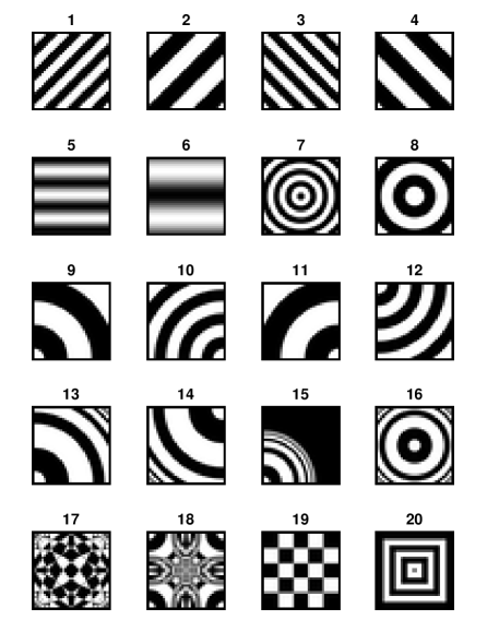
Figure 2: Images that were used for numerical simulations.

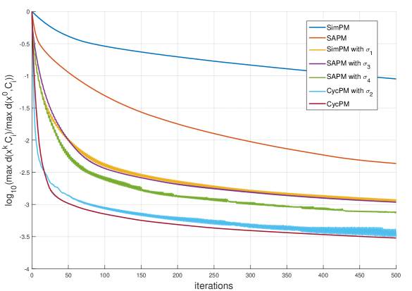
Figure 3: Numerical behavior for simultaneous, cyclic and string averaging projection methods described in (5.2)–(5.7). We recall that for SAPM we consider $N=84$ strings, most of them of length $m=10$. Each curve represents the average of the quantity (5.8) obtained for all 20 test problems presented in Figure 2.

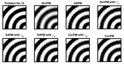
Figure 4: Solutions obtained for problem number 10 after 500 iterations of simultaneous, cyclic and string averaging projection methods described in (5.2)–(5.7).

Acknowledgments. This research was supported in part by the Israel Science Foundation (Grants no. 389/12 and 820/17), by the Fund for the Promotion of Research at the Technion and by the Technion General Research Fund. The first and the fourth authors were partially supported by the Austria–Israel Academic Network in Innsbruck (AIANI).

References

- [1] A. Aleyner and S. Reich, Block-iterative algorithms for solving convex feasibility problems in Hilbert and in Banach spaces, J. Math. Anal. Appl., 343 (2008), pp. 427–435.
- [2] K. Aoyama and F. Kohsaka, Viscosity approximation process for a sequence of quasinonexpansive mappings, Fixed Point Theory Appl., 2014:17 (2014).
- [3] N. Asuni and A. Giachetti, Testimages: A large data archive for display and algorithm testing, Journal of Graphics Tools, 17 (2013), pp. 113–125.
- [4] N. Asuni and A. Giachetti, Testimages: a large-scale archive for testing visual devices and basic image processing algorithms, in Smart Tools and Apps for Graphics - Eurographics Italian Chapter Conference, A. Giachetti, ed., The Eurographics Association, 2014, doi:10.2312/stag.20141242.
- [5] C. Bargetz, S. Reich, and R. Zalas, Convergence properties of dynamic string-averaging projection methods in the presence of perturbations, Numer. Algorithms, 77 (2018), pp. 185–209.
- [6] H. H. Bauschke and J. M. Borwein, On projection algorithms for solving convex feasibility problems, SIAM Rev., 38 (1996), pp. 367–426.
- [7] H. H. Bauschke and P. L. Combettes, Convex analysis and monotone operator theory in Hilbert spaces, CMS Books in Mathematics/Ouvrages de Mathématiques de la SMC, Springer, New York, 2011. With a foreword by Hédy Attouch.
- [8] H. H. Bauschke, P. L. Combettes, and S. G. Kruk, Extrapolation algorithm for affine-convex feasibility problems, Numer. Algorithms, 41 (2006), pp. 239–274.
- [9] H. H. Bauschke, E. Matoušková, and S. Reich, Projection and proximal point methods: convergence results and counterexamples, Nonlinear Anal., 56 (2004), pp. 715–738.
- [10] H. H. Bauschke, D. Noll, and H. M. Phan, Linear and strong convergence of algorithms involving averaged nonexpansive operators, J. Math. Anal. Appl., 421 (2015), pp. 1–20.
- [11] J. M. Borwein, G. Li, and M. K. Tam, Convergence rate rnalysis for averaged fixed point iterations in common fixed point problems, SIAM J. Optim., 27 (2017), pp. 1–33.
- [12] F. E. Browder and W. V. Petryshyn, The solution by iteration of nonlinear functional equations in Banach spaces, Bull. Amer. Math. Soc., 72 (1966), pp. 571–575.
- [13] D. Butnariu, R. Davidi, G. T. Herman, and I. G. Kazantsev, Stable convergence behavior under summable perturbations of a class of projection methods for convex feasibility and optimization problems, IEEE Journal of Selected Topics in Signal Processing, 1 (2007), pp. 540–547.
- [14] D. Butnariu, S. Reich, and A. J. Zaslavski, Stable convergence theorems for infinite products and powers of nonexpansive mappings, Numer. Funct. Anal. Optim., 29 (2008), pp. 304–323.
- [15] A. Cegielski, Iterative methods for fixed point problems in Hilbert spaces, vol. 2057 of Lecture Notes in Mathematics, Springer, Heidelberg, 2012.
- [16] A. Cegielski, Application of quasi-nonexpansive operators to an iterative method for variational inequality, SIAM J. Optim., 25 (2015), pp. 2165–2181.
- [17] A. Cegielski and Y. Censor, Extrapolation and local acceleration of an iterative process for common fixed point problems, J. Math. Anal. Appl., 394 (2012), pp. 809–818.
- [18] A. Cegielski and N. Nimana, Extrapolated cyclic subgradient projection methods for the convex feasibility problems and their numerical behavior, (preprint).
- [19] A. Cegielski, S. Reich, and R. Zalas, Regular Sequences of Quasi-Nonexpansive Operators and Their Applications, SIAM J. Optim., 28 (2018), pp. 1508–1532.
- [20] A. Cegielski and R. Zalas, Methods for variational inequality problem over the intersection of fixed point sets of quasi-nonexpansive operators, Numer. Funct. Anal. Optim., 34 (2013), pp. 255–283.
- [21] A. Cegielski and R. Zalas, Properties of a class of approximately shrinking operators and their applications, Fixed Point Theory, 15 (2014), pp. 399–426.
- [22] Y. Censor, T. Elfving, and G. T. Herman, Averaging strings of sequential iterations for convex feasibility problems, in Inherently parallel algorithms in feasibility and optimization and their applications (Haifa, 2000), vol. 8 of Stud. Comput. Math., North-Holland, Amsterdam, 2001, pp. 101–113.
- [23] Y. Censor and R. Mansour, New Douglas-Rachford algorithmic structures and their convergence analyses, SIAM J. Optim., 26 (2016), pp. 474–487.
- [24] Y. Censor and A. Segal, Iterative projection methods in biomedical inverse problems, in Mathematical methods in biomedical imaging and intensity-modulated radiation therapy (IMRT), vol. 7 of CRM Series, Ed. Norm., Pisa, 2008, pp. 65–96.
- [25] Y. Censor and E. Tom, Convergence of string-averaging projection schemes for inconsistent convex feasibility problems, Optim. Methods Softw., 18 (2003), pp. 543–554.
- [26] Y. Censor and A. J. Zaslavski, Convergence and perturbation resilience of dynamic string-averaging projection methods, Comput. Optim. Appl., 54 (2013), pp. 65–76.
- [27] P. L. Combettes, The convex feasibility problem in image recovery, vol. 95 of Advances in Imaging and Electron Physics, Elsevier, 1996, pp. 155–270.
- [28] P. L. Combettes, Hilbertian convex feasibility problem: convergence of projection methods, Appl. Math. Optim., 35 (1997), pp. 311–330.
- [29] G. Crombez, Finding common fixed points of strict paracontractions by averaging strings of sequential iterations, J. Nonlinear Convex Anal., 3 (2002), pp. 345–351.
- [30] L. T. Dos Santos, A parallel subgradient projections method for the convex feasibility problem, J. Comput. Appl. Math., 18 (1987), pp. 307–320.
- [31] S. D. Flåm and J. Zowe, Relaxed outer projections, weighted averages and convex feasibility, BIT, 30 (1990), pp. 289–300.
- [32] K. Goebel and S. Reich, Uniform convexity, hyperbolic geometry, and nonexpansive mappings, vol. 83 of Monographs and Textbooks in Pure and Applied Mathematics, Marcel Dekker, Inc., New York, 1984.
- [33] K. C. Kiwiel and B. Łopuch, Surrogate projection methods for finding fixed points of firmly nonexpansive mappings, SIAM J. Optim., 7 (1997), pp. 1084–1102.
- [34] V. I. Kolobov, S. Reich, and R. Zalas, Weak, strong, and linear convergence of a double-layer fixed point algorithm, SIAM J. Optim., 27 (2017), pp. 1431–1458.
- [35] D. R. Luke, N. H. Thao, and M. K. Tam, Implicit Error Bounds for Picard Iterations on Hilbert Spaces, Vietnam J. Math., 46 (2018), pp. 243–258.
- [36] T. Nikazad, M. Abbasi, and M. Mirzapour, Convergence of string-averaging method for a class of operators, Optim. Methods Softw., 31 (2016), pp. 1189–1208.
- [37] T. Nikazad and M. Mirzapour, Extrapolation of relaxed cutter operators for convex feasibility problem, in 8th International Conference of the Iranian Soceity of Operations Research, Ferdowsi University of Mashhad, May 21-22, 2015, 2015, pp. 171–174.
- [38] T. Nikazad and M. Mirzapour, Generalized relaxation of string averaging operators based on strictly relaxed cutter operators, J. Nonlinear Convex Anal., 18 (2017), pp. 431–450.
- [39] Z. Opial, Weak convergence of the sequence of successive approximations for nonexpansive mappings, Bull. Amer. Math. Soc., 73 (1967), pp. 591–597.
- [40] C. L. Outlaw, Mean value iteration of nonexpansive mappings in a Banach space, Pacific J. Math., 30 (1969), pp. 747–750.
- [41] W. V. Petryshyn and T. E. Williamson, Jr., Strong and weak convergence of the sequence of successive approximations for quasi-nonexpansive mappings, J. Math. Anal. Appl., 43 (1973), pp. 459–497.
- [42] G. Pierra, Decomposition through formalization in a product space, Math. Programming, 28 (1984), pp. 96–115.
- [43] S. Reich and Z. Salinas, Metric convergence of infinite products of operators in Hadamard spaces, J. Nonlinear Convex Anal., 18 (2017), pp. 331–345.
- [44] S. Reich and R. Zalas, A modular string averaging procedure for solving the common fixed point problem for quasi-nonexpansive mappings in Hilbert space, Numer. Algorithms, 72 (2016), pp. 297–323.
- [45] S. Reich and A. J. Zaslavski, An example concerning bounded linear regularity of subspaces in Hilbert space, Bull. Aust. Math. Soc., 89 (2014), pp. 217–226.
- [46] S. Reich and A. J. Zaslavski, Porosity and the bounded linear regularity property, J. Appl. Anal., 20 (2014), pp. 1–6.
- [47] A. J. Zaslavski, Dynamic string-averaging projection methods for convex feasibility problems in the presence of computational errors, J. Nonlinear Convex Anal., 15 (2014), pp. 623–636.
- [48] A. J. Zaslavski, Approximate solutions of common fixed-point problems, vol. 112 of Springer Optimization and Its Applications, Springer, 2016.
- [49] X. Zhao, K. F. Ng, C. Li, and J.-C. Yao, Linear regularity and linear convergence of projection-based methods for solving convex feasibility problems, Applied Mathematics & Optimization, (2017), doi:10.1007/s00245-017-9417-1.