Abstract

Several well-established benchmark predictors exist for Value-at-Risk (VaR), a major instrument for financial risk management. Hybrid methods combining AR-GARCH filtering with skewed-$t$ residuals and the extreme value theory-based approach are particularly recommended. This study introduces yet another VaR predictor, G-VaR, which follows a novel methodology. Inspired by the recent mathematical theory of sublinear expectation, G-VaR is built upon the concept of model uncertainty, which in the present case signifies that the inherent volatility of financial returns cannot be characterized by a single distribution but rather by infinitely many statistical distributions. By considering the worst scenario among these potential distributions, the G-VaR predictor is precisely identified. Extensive experiments on both the NASDAQ Composite Index and S&P500 Index demonstrate the excellent performance of the G-VaR predictor, which is superior to most existing benchmark VaR predictors.

KEYWORDS: Empirical finance, G-normal distribution, Model uncertainty, Sublinear expectation, Value-at-Risk.

JEL Classification: C58, G32.

1 Introduction

Since its birth at J.P. Morgan in the 1990s, value-at-risk (VaR) has become one of the most used (if not THE most used) instruments for assessing downside risk in financial markets. Every unit of risk management in today’s financial industry routinely implements several VaR indicators to monitor its business (Jorion, 2007). The regulatory authorities also incorporate VaR measures into their recommendations to the banking industry (Basel Accords I-III), which has accelerated the spread of VaR.

The success of VaR methodology is also backed up by a rich body of literature in which the methodology is carefully evaluated and discussed in different model settings and for different markets and products. The literature on VaR is voluminous and includes several specialized books. Also any textbook treating financial econometrics or risk management will have a chapter dedicated to VaR. For an up-to-date account of this literature, the reader is referred to the recent review papers by Kuester et al. (2006), Jorion (2010), Abad et al. (2014), Nadarajah and Chan (2016), and Zhang and Nadarajah (2017), among others. In particular, Table 4 in Abad et al. (2014) lists as many as fourteen papers that survey and compare different VaR methodologies through empirical studies. Further, by focusing on univariate observations, Kuester et al. (2006) offer a rich review of mainstream VaR measures and provide an extensive empirical comparison of those measures in terms of their prediction power using the daily NASDAQ Composite Index. The general conclusion they draw (see also Abad et al., 2014) is that whatever method is used for VaR modeling, the predictions are always improved, most of the time considerably improved, by applying that method to residuals filtered by an AR-GARCH model instead of the original series $(r_{t})$. For example, one of the best performers is obtained by applying extreme value theory (EVT) to the residuals of AR-GARCH fit using skewed-$t$ innovations (AR-GARCH St-EVT). Kuester et al. (2006) conclude that, at least for the NASDAQ Composite Index, “conditionally heteroskedastic models yield acceptable forecasts” and that the conditional skewed-$t$ (AR-GARCH-St) together with the conditional skewed-$t$ coupled with EVT (AR-GARCH-St-EVT) perform best in general.

In this paper, we present an entirely new type of VaR. Our methodology is inspired by a rigorous mathematical theory called nonlinear expectation. The theory of nonlinear expectation was originally introduced in Peng (2004, 2006, 2008, 2019). The part of the theory relevant to VaR prediction is detailed in the appendix. When applied to analysis of a time-series of returns $\{r_{t}\}$, the central concept of nonlinear expectation theory is an infinite family of distributions inherent in the return series $\{r_{t}\}$. Traditional econometric modeling commonly assumes that returns, at least during certain time periods, obey one stochastic process governed by one stochastic-process model $P_{0}$. The task of the econometrician is to infer this unknown, but true, $P_{0}$. The distribution can be parametric, as in an AR-ARCH model (with skewed-$t$ or normal innovations), or made up by a family of conditional mixture distributions (see Section 2). It can also be fully nonparametric without any particular model specification, as in the historical simulation (HS) approach to VaR prediction. However, a unique stochastic model is assumed so far for the returns $\{r_{t}\}$. The point of view of nonlinear expectation theory is radically different: instead of assuming the existence of one unique model $P_{0}$, it views returns as originating from a large number of different models, say $\{P_{\theta}\}_{\theta\in\Theta}$, and this family of potential models is indeed infinite (here, $\Theta$ denotes some imprecise index set). The rationale is that data under investigation such as return series are of a complex nature such that no single stochastic model or distribution can serve as a perfect model: model uncertainty has to be considered, and any statistical inference has to take into account such uncertainty. We name this vision of complex data and the implied methodology data analysis under model uncertainty.

The concept of model uncertainty, sometimes also referred to as model ambiguity, has taken a long time to emerge. An early attempt in this direction was made in the area of robust statistics, where it was argued that a statistical procedure (e.g. parameter estimation or hypothesis testing) can gain robustness by assuming that the data follow not a single distribution but rather a family of distributions $\{F_{\theta}\}_{\theta\in\Theta}$ (see Huber, 1981; Walley, 1991). By allowing a variable range between two extreme values $\mathrm{\sigma}_{min}$ and $\mathrm{\sigma}_{max}$ for volatility of a stock, Avellaneda et al. (1995) presented a model for pricing and hedging derivative securities and option portfolios. When the volatility is unknown and takes value in some convex region that can vary with the price process and time, Lyons (1995) introduced optimal and risk-free strategies for intermediaries in such markets to meet their obligations. Peng (1997) later proposed a formal mathematical approach to model uncertainty, with a nonlinear expectation called $g$-expectation introduced to develop the concept of mean uncertainty and its associated mathematical tools. The $g$-expectation concept was then adopted by Chen and Epstein (2002) to describe the continuous-time inter-temporal version of multiple-priors utility. In particular, they established a separate premium for ambiguity on top of the traditional premium for risk. In addition, Epstein and Ji (2013) formulated a model of utility in a continuous-time framework that captures aversion to ambiguity about both the volatility and the mean of returns via the theory of sublinear expectation (SLE). Note that sublinear expectation is a useful form of nonlinear expectation reinforced by the addition of a sub-addivity property. All of the above theories formalize an inherent family of distributions involving a set of probability measures $\{P_{\theta}\}_{\theta\in\Theta}$, not just one probability measure $P_{0}$, that governs the statistical distributions of a dataset. In related work, Artzner et al. (1999) proposed the concept of coherent risk measures, which focused on measurement of both market risks and nonmarket risks, see also Föllmer and Schied (2011).

Although the vision of model uncertainty has been formalized through the rigorous mathematical theory of SLE, its implications for real data analysis have not been fully explored. Early work by Huber (Huber, 1981) studied the model uncertainty in the area of robust statistics. Cont (2006) considered a quantitative framework for defining model uncertainty in option pricing models, and illustrated the difference between model uncertainty and the more common notion of ”market risk” through examples. By distinguishing estimation risk and misspecification risk, Kerkhof et al. (2010) proposed a procedure to take model risk into account in the computation of capital reserves which can be used to address Value-at-Risk and expected shortfall. To the best of our knowledge, the present paper on VaR prediction constitutes the first attempt at real-life data analysis under SLE-based model uncertainty. The implementation of SLE theory herein leads to a new type of VaR predictor called $G$-VaR. Loosely speaking, as long as VaR prediction is concerned and to give model uncertainty in the form of an infinite family of probability models $\{P_{\theta}\}_{\theta\in\Theta}$, G-VaR concentrates on prediction under the worst scenario among all potential models $\{P_{\theta}\}$. Extensive empirical analyses of two major market indexes, namely, the NASDAQ Composite Index and S&P 500 Index, establish the superiority of the new G-VaR predictions over several benchmark VaR predictors that are among the best performers reported in Kuester et al. (2006). The uniform superiority of G-VaR in these empirical studies is truly astonishing. One a posteriori explanation is that these return data do have the kind of complex nature that can be better understood through the lens of model uncertainty that had led to the G-VaR predictor.

The remainder of the paper is organized as follows. Section 2 briefly reviews several benchmark predictors for the VaR of return series. Section 3 introduces the concepts of distribution family as model uncertainty and G-normal distribution. Section 4 contains the main technical contribution of the paper. The new VaR predictor, i.e. G-VaR, is introduced under model uncertainty and its theoretical properties established. The implementation of G-VaR is presented in Section 5, in which consistent estimators are proposed for the parameters involved in the G-VaR predictor. Note that this implementation is far non trivial and Section 5 contains the main methodological contribution of the paper. Section 6 reports the empirical results of the G-VaR predictor for the NASDAQ Composite Index and S&P 500 Index, with extensive comparison made with the benchmark VaR predictors reviewed in Section 2, including the AR(1)-GARCH(1,1)-Normal, AR(1)-GARCH(1,1)-Skewed-t and AR(1)-GARCH(1,1)-Skewed-t-EVT predictors. Finally, Section 7 concludes.

2 A brief review of benchmark predictors for VaR

Before introducing our new methodology, we first give a brief review of several of the well-documented VaR predictors described in Kuester et al. (2006), as they will serve as benchmarks for comparison with the new VaR predictor proposed herein. As historical references for these VaR measures can be found in the earlier review paper, only a few key references are indicated in this brief review. Here, $(r_{t})$ denotes a univariate time-series for which VaR prediction is required. In most common situations, the series represents the daily returns of a market, or price of a stock or product.

(i) The Historical Simulation method. This traditional method uses sample quantiles from historical data to predict VaR. The method is well documented in classic books such as Dowd (2002) and Christoffersen (2003).

A variant of HS is filtered historical simulation (FHS), whereby the sample quantiles are calculated from filtered residuals using a parametric model such as the AR-GARCH model. Classical references on FHS include Barone-Adesi et al. (1999, 2002).

(ii) The method of Peaks over Thresholds using EVT. EVT provides a method for estimating the high upper quantiles of a variable $X$, say quantiles $x_{\alpha}$ such that $\overline{F}_{X}(x)=P(X>x_{\alpha})=\alpha$ for some small tail probability $\alpha<0.1$. From sample data, one obtains an empirical quantile $u$, the threshold, such that $P(X>u)\approx 0.1$. Also those values above threshold $u$ provide a sample for the “survival distribution” $(X|X>u)$. EVT ensures that for a large enough $u$, the survival distribution can be approximated by a generalized Pareto distribution (GPD) that depends on a pair of shape-scale parameters $(\beta,\xi)$ (Pickands, 1975; Embrechts et al., 1997). This GPD is thus identified using the sample, which leads to an estimate for the initial tail probability $\overline{F}_{X}(x_{\alpha})$ for all $x_{\alpha}>u$.

For VaR prediction, the above procedure is applied to the available data $\{X_{s}=-r_{s},~{}s<t\}$ to find the corresponding upper quantile $x_{\alpha}$. The negative operation is used here, as EVT considers upper quantiles whereas VaR targets lower quantiles. Then, the prediction for VaR is $\widehat{\text{VaR}}_{\alpha}(t)=-x_{\alpha}$ for all risk levels $\alpha<0.1$. Empirical studies on VaR predictions using EVT can be found in McNeil and Frey (2000) and Kuester et al. (2006).

(iii) The method by AR-GARCH filtering (AR-GARCH). Here the returns are assumed to follow a mean-variance decomposition of type

$$r_{t}=\mu_{t}+\sigma_{t}z_{t},$$ (2.1)

where the mean process $(\mu_{t})$ follows an AR model (or, more generally, an ARMA model) and the residual is modeled by a GARCH process (Bollerslev, 1986) with independent and identically distributed (i.i.d.) innovations $(z_{t})$. Common choices for the distribution $f_{z}$ of the innovations $(z_{t})$ are (i) standard normals, (ii) Student’s $t$-distributions, and (iii) skewed $t$-distributions.

Once the model (2.1) is fitted, a parametric estimate of the distribution $f_{z}$ is obtained, say $\hat{f}_{z}$, which leads to an estimated quantile function, say $\hat{Q}_{\alpha}(z)$ (for any given risk level $\alpha$). A level-$\alpha$ VaR prediction at time $t$ is thus defined as

$$\widehat{\text{VaR}}_{\alpha}(t)=-\left\{\hat{\mu}_{t}+\hat{\sigma}_{t}\hat{Q}_{\alpha}(z)\right\}.$$

(iv) The method of Conditional Mixture Modeling. In this approach, conditional to the information set ${\cal F}_{t-1}$ at time $t$, the return $r_{t}$ follows a mixture distribution with $n$ components, each of which has a constant mean parameter $\mu_{j}$ ($1\leq j\leq n$) and time-varying volatility (variance) parameter $\sigma^{2}_{j,t}$ ($1\leq j\leq n$). Moreover, the $n$-dimensional volatility process $\bm{\sigma}_{t}^{2}=(\sigma^{2}_{1,t},\ldots,\sigma^{2}_{n,t})$ obeys a multidimensional GARCH equation. Here, the distributions of the mixture components are usually taken to be normal distributions or generalized exponential distributions (GED). More references to this approach can be found in Haas et al. (2004).

(v) The method by Quantile Regression. Here a regression model is used to predict the VaR at time $t$ using some predictable covariates ${\bf X}_{t}\in{\cal F}_{t-1}$; see Koenker and Bassett (1978) and Chernozhukov and Umantsev (2001). Later, Engle and Manganelli (2004) proposed CAViaR models, where the quantiles (or VaRs) follow an autoregressive model without any exogeneous covariate.

3 G-normal distribution

When measuring the risk in a financial time-series $\{X_{t}\}_{0\leq t\leq T}$, it is commonly assumed that the data follow a certain distribution $F_{0}$, and the aim is to estimate or approximate the “true” distribution $F_{0}$ or some of its characteristics such as VaR. As we saw in the survey in Section 2, many different VaR measures exist in the literature, including HS, EVT-VaR and their AR-GARCH-filtered variants. Now we view the data $\{X_{t}\}_{0\leq t\leq T}$ as possessing a complex nature governed not by one distribution $F_{0}$ but rather by an infinite family of distributions $\{F_{\theta}\}_{\theta\in\Theta}$, each of them capturing some properties of the data.

How can the VaR concept be extended to a new framework in which an infinite family of (unknown) distributions governs the data? This paper provides an answer to this general question. To proceed, some meaningful characteristics of the family $\{F_{\theta}\}_{\theta\in\Theta}$ need to be identified. Consider the simplest features of the distributions, namely, their mean $\mu$ and variance $\sigma^{2}$. In general, these features are time-varying. Here, we consider a simple case, where mean $\mu$ is constant (independent of time) and variance $\sigma^{2}$ is time-varying within some interval $[\underline{\sigma}^{2},\overline{\sigma}^{2}]$. In the following, the interval $[\underline{\sigma}^{2},\overline{\sigma}^{2}]$ is used to characterize the unknown family of distributions $\{F_{\theta}\}_{\theta\in\Theta}$. For a given canonical probability space $(\Omega,\mathcal{F},P)$, $\Omega=C([0,T])$, and Brownian motion $\{B_{t}\}_{0\leq t\leq T}$, we define the probability measures $P_{\theta}$ as follows. For $A\in\mathcal{F}$,

$$P_{\theta}(A)=P\circ Y_{\theta}^{-1}(A)=P(Y_{\theta}\in A),$$

where

$$Y_{\theta}(\cdot)=\int_{0}^{\centerdot}\theta_{s}dB_{s},\quad\theta\in\Theta=L^{2}_{{\cal F}}(\Omega\times[0,T],[\underline{\sigma},\overline{\sigma}]),$$

where $\Theta$ is the set of all progressively measurable processes taking value on $[\underline{\sigma},\overline{\sigma}]$ The collection of $P_{\theta}$s is denoted as $\{P_{\theta}\}_{\theta\in\Theta}$. Let the mean $\mu$ be $0$ and the distribution of $\{X_{t}\}_{0\leq t\leq T}$ under $P_{\theta}$ be $F_{\theta}$. Thus, this infinite family of stochastic process distributions $\{F_{\theta}\}_{\theta\in\Theta}$ is chosen as the family governing the dataset $\{X_{t}\}_{0\leq t\leq T}$. In this paper, we use the so-called G-normal distribution $N(0,[\underline{\sigma}^{2},\overline{\sigma}^{2}])$ to represent the family $\{F_{\theta}\}_{\theta\in\Theta}$.

Precisely, the expectations of data $\{X_{t}\}_{0\leq t\leq T}$ under $\{P_{\theta}\}_{\theta\in\Theta}$ are

$${E}_{\theta}[\phi(X_{t})]=\int_{R}\phi(x)dF_{\theta}(x),$$ (3.1)

where $\phi\in C_{l.Lip}(\mathbb{R},\mathbb{R})$ is a test function describing the statistic of the data $X_{t}$ that we are interested in. With VaR prediction in view, we concentrate our analysis on the worst-case expectation of $X_{t}$ under $\{P_{\theta}\}_{\theta\in\Theta}$, that is,

$$\mathbb{E}[\phi(X_{t})]=\sup_{\theta\in\Theta}E_{\theta}[\phi(X_{t})].$$ (3.2)

In general, it is difficult to determine worst-case expectation $\mathbb{E}[\phi(X_{t})]$. There is, however, a situation in which it can be explicitly determined, as shown below.

Assumption 3.1.

Suppose that $\{X_{t}\}_{0<t<T}$ satisfies the following stochastic differential equation,

$$dX_{t}=\theta_{t}dB_{t},\quad X_{0}=x,$$

under $P_{\theta}$, $\theta\in\Theta=L^{2}_{{\cal F}}(\Omega\times[0,T],[\underline{\sigma},\overline{\sigma}])$.

For a given $\phi$, we can prove that $u(t,x)=\mathbb{E}[\phi(X_{t})]$ satisfies the following partial differential equation (PDE),

$$\partial_{t}u(t,x)-G(\partial_{xx}^{2}u)=0,\ t\geq 0,\ x\in\mathbb{R},$$ (3.3)

where the function $G(\cdot)$ is defined as

$$G(a)=\frac{1}{2}\left(\overline{\sigma}^{2}a^{+}-\underline{\sigma}^{2}a^{-}\right),\quad a^{+}=\max(a,0),\quad\text{and}\quad a^{-}=\max(-a,0).$$ (3.4)

If, in addition, $\phi(\cdot)$ is convex on $\mathbb{R}$, then the following explicit solution exists for the equation (3.3):

$$u(t,x)=\int_{-\infty}^{x}\phi(y)\frac{1}{\sqrt{2\pi t\overline{\sigma}^{2}}}\exp(\frac{y^{2}}{2t\overline{\sigma}^{2}})dy.$$

In this case, we can see that the convex function $u(t,x)$ will reach the maximum at parameter $\overline{\sigma}$. Similarly, if $\phi(\cdot)$ is concave on $\mathbb{R}$, then the explicit solution becomes

$$u(t,x)=\int_{-\infty}^{x}\phi(y)\frac{1}{\sqrt{2\pi t\underline{\sigma}^{2}}}\exp(\frac{y^{2}}{2t\underline{\sigma}^{2}})dy.$$

As a time-series of returns $\{X_{t}\}_{0\leq t\leq T}$ is typically centered whereas its volatility (variance) is time-varying, we will hereafter assume that it satisfies Assumption 3.1 under model uncertainty $\{P_{\theta}\}_{\theta\in\Theta}$ and follows a G-normal distribution $N(0,[\underline{\sigma}^{2},\overline{\sigma}^{2}])$ (the reader is reminded that this is not a classical probability distribution). The definitions of maximal distribution and unbiased estimator are given as follows:

Definition 3.1.

(Maximal distribution) A random variable $\eta$ on a sublinear expectation space $(\Omega,\mathcal{H},\mathbb{E})$ is called maximally distributed if there exists an interval $[\underline{\mu},\overline{\mu}]\subset\mathbb{R}$ such that

$$\mathbb{E}[\phi(\eta)]=\max_{y\in[\underline{\mu},\overline{\mu}]}\phi(y),\quad\forall\phi\in C_{l.Lip}(\mathbb{R}).$$

Definition 3.2.

Let $X_{1},\cdots,X_{n}$ be i.i.d. sample (under SLE) of size $n$ from the maximal distribution with interval $[\underline{\mu},\overline{\mu}]$. We say $f(X_{1},\cdots,X_{n})$ is an unbiased estimator of $\underline{\mu}$ or $\overline{\mu}$ if $\mathbb{E}[f(X_{1},\cdots,X_{n})]=\underline{\mu}$ or $\mathbb{E}[f(X_{1},\cdots,X_{n})]=\overline{\mu}$, respectively.

4 G-VaR: a new VaR approach under model uncertainty

First recall that, given $\alpha\in(0,1)$, the $\text{VaR}_{\alpha}$ at the risk level $\alpha$ of a financial asset $X$ is the negative of the level-$\alpha$ quantile of $X$; that is

$$\text{VaR}_{\alpha}(X)=-\inf\{x~{}:~{}F(x)>\alpha\},$$ (4.1)

where $F(x)=P(X\leq x)$ is the cumulative distribution function of $X$.

4.1 Robust VaR

Consider a risky position $X$ under model uncertainty represented by a family of distributions $\{F_{\theta}(x)\}_{\theta\in\Theta}$. The VaR of $X$ under each $F_{\theta}$ is

$$\text{VaR}^{\theta}_{\alpha}(X)=-\inf\{x~{}:~{}F_{\theta}(x)>\alpha\}.$$

Under the distribution family considered here, it is important to design a VaR measure that can protect itself against risk. Note that risk here takes a quite general form; that is, no specific form or prior information is available on this family of distributions. This generality is aligned with real market situations in which risk factors are always difficult, and perhaps impossible, to capture precisely. Hence, any particular form or modeling of the sources of these risks could be misleading. Accordingly, it becomes natural to consider a worst-case scenario for VaR. Formally, the worst-case VaR of $X$ is here defined as

$$\text{VaR}^{*}_{\alpha}(X):=\sup_{\theta\in\Theta}\text{VaR}^{\theta}_{\alpha}(X).$$ (4.2)

In the empirical study in Section 6, it will be shown that, despite its conservative spirit, consideration of a worst-case scenario, allows the new VaR to capture the risks in asset returns very efficiently.

The worst-case VaR (4.2) has several simple properties. Let

$$\hat{F}(x):=\sup_{\theta\in\Theta}F_{\theta}(x).$$ (4.3)

For each $\theta$, we have

$$\text{VaR}^{\theta}_{\alpha}(X)\leq-\inf\{x~{}:~{}\hat{F}(x)>\alpha\}=:\text{VaR}^{\hat{F}}_{\alpha}(X),$$

such that $\text{VaR}^{*}_{\alpha}(X)\leq\text{VaR}^{\hat{F}}_{\alpha}(X)$.

Remark 4.1.

It is clear that $\hat{F}$ is a right continuous function. If, in addition, $\{F_{\theta}\}_{\theta\in\Theta}$ is weakly compact,then it is easy to prove that

$$\lim_{x\to-\infty}\hat{F}(x)=0,\quad\text{and}\quad\lim_{x\to\infty}\hat{F}(x)=1.$$

Thus in this case, $\hat{F}$ is still a probability distribution function.

Proposition 4.1.

Given a risky position $X$ and a family of distributions $\{F_{\theta}(x)\}_{\theta\in\Theta}$ that is weakly compact. Then,

$$\text{VaR}^{*}_{\alpha}(X):=\sup_{\theta\in\Theta}\text{VaR}^{\theta}_{\alpha}(X)=\text{VaR}^{\hat{F}}_{\alpha}(X).$$

Proof.

It is clear that $\text{VaR}^{*}_{\alpha}(X)\leq\text{VaR}^{\hat{F}}_{\alpha}(X)$. To prove the reverse inequality, it suffices to find an $\tilde{F}\in\{F_{\theta}(x)\}_{\theta\in\Theta}$ such that

$$\text{VaR}^{\hat{F}}_{\alpha}(X)=\text{VaR}^{\tilde{F}}_{\alpha}(X).$$

Because $\hat{F}(x)$ is a right continuous non-decreasing function, we can find an $x_{\alpha}\in(-\infty,\infty)$ such that

$$\hat{F}(x_{\alpha})\geq\alpha>\hat{F}(x),\ \text{for each}\ x<x_{\alpha}.$$

Let $\{F_{\theta_{i}}\}_{i=1}^{\infty}$ be a subsequence of $\{F_{\theta}\}_{\theta\in\Theta}$ such that $F_{\theta_{i}}(x_{\alpha})\to\hat{F}(x_{\alpha})$. Because $\{F_{\theta}(x)\}_{\theta\in\Theta}$ is weakly compact, there exists a subsequence of $\{F_{\theta_{i_{k}}}\}_{k=1}^{\infty}$ such that $\{F_{\theta_{i_{k}}}\}_{k=1}^{\infty}$ weakly converges to $\tilde{F}\in\{F_{\theta}(x)\}_{\theta\in\Theta}$. From

$$\hat{F}(x_{\alpha})=\lim_{k\to\infty}F_{\theta_{i_{k}}}(x_{\alpha})\leq\tilde{F}(x_{\alpha})\leq\hat{F}(x_{\alpha}),$$

it follows that $\tilde{F}(x_{\alpha})=\hat{F}(x_{\alpha})$. Further, for each $x<x_{\alpha}$, $\tilde{F}(x)\leq\hat{F}(x)<\hat{F}(x_{\alpha})$, namely,

$$-\text{VaR}^{\hat{F}}_{\alpha}(X)=x_{\alpha}=\inf\{x~{}:~{}\tilde{F}(x)>\alpha\}=-\text{VaR}^{\hat{F}}_{\alpha}(X).$$

The proof is complete. ∎

4.2 G-VaR

Based on Proposition 4.1, we now introduce the concept of G-VaR under the family of distributions $\{F_{\theta}\}_{\theta\in\Theta}$ for a risky asset $X$ that follows a G-normal distribution $N(0,[\underline{\sigma}^{2},\overline{\sigma}^{2}])$ depending on two positive parameters $(\underline{\sigma},\overline{\sigma})$. More precisely, G-VaR is defined by replacing the classical distribution function $F(x)$ in (4.1) with G-expectation $\mathbb{E}[1_{X\leq x}]$, that is,

$$\text{G-VaR}_{\alpha}(X):=-\inf\{x\in\mathbb{R}:\mathbb{E}[1_{X\leq x}]>\alpha\}.$$ (4.4)

Note that if model uncertainty were absent, the family $\{F_{\theta}\}_{\theta\in\theta}$ would reduce to a single distribution $F$, and G-VaR would coincide with the traditional VaR in (4.1). Furthermore, as $X$ follows a G-normal distribution, we have

$$\hat{F}(x)=\mathbb{E}[1_{X\leq x}]=u(t,x)|_{t=1},$$

where $u$ is the solution to the nonlinear heat equation (3.3), with Cauchy initial condition

$$\lim_{t\to 0}u(t,x)=1_{(0,\infty)}(x).$$ (4.5)

By Proposition A.1, function $\hat{F}$ has the following closed-form expressions.

$$\hat{F}(x)=\int_{-\infty}^{x}\frac{\sqrt{2}}{(\overline{\sigma}+\underline{\sigma})\sqrt{\pi}}\left[e^{-\frac{y^{2}}{2\overline{\sigma}^{2}}}I(y\leq 0)+e^{-\frac{y^{2}}{2\underline{\sigma}^{2}}}I(y>0)\right]dy,$$

where $I(A)$ denotes the indicator function of a set $A$. Moreover, evaluating the integral leads to the following more explicit form of the function;

$$\hat{F}(x)=\frac{2\overline{\sigma}}{\overline{\sigma}+\underline{\sigma}}\Phi(\frac{x}{\overline{\sigma}})\ I(x\leq 0)+\left\{1-\frac{2\underline{\sigma}}{\overline{\sigma}+\underline{\sigma}}\Phi(-\frac{x}{\underline{\sigma}})\right\}\ I(x>0),$$ (4.6)

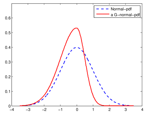
where $\Phi$ denotes the distribution function of the standard normal. This G-normal distribution has a negative mean $\sqrt{\frac{2}{\pi}}(\underline{\sigma}-\overline{\sigma})$, and a negative skew. As an example, the G-normal density function with parameters $(\underline{\sigma},\overline{\sigma})=(0.5,1)$ is compared to the standard normal density in Figure 1. Furthermore, as $\hat{F}$ is monotonically increasing, the G-VaR in (4.4) is equal to

$$\text{G-VaR}_{\alpha}(X)=-{\hat{F}}^{-1}(\alpha).$$ (4.7)

Insert Figure 1 around here

4.3 A simple interpretation of G-VaR and some general comments

Although the G-VaR is derived through the fairly sophisticated theory of SLE and related G-normal distribution, its final implementation shown in equations (4.6) and (4.7) has a simple interpretation. First of all, a G-normal distribution we assumed for the asset $X$ can be intuitively related to an infinite family of normal distributions $\{N(0,\sigma^{2}):\,\sigma^{2}\in[{\underline{\sigma}}^{2},{\overline{\sigma}}^{2}]\}$. Therefore the volatility interval $[{\underline{\sigma}}^{2},{\overline{\sigma}}^{2}]$ corresponds to the model uncertainty considered here. As G-VaR is positive ($\alpha<0.5$), (4.7) can be rewritten as a normal VaR:

$$\text{G-VaR}_{\alpha}(X)=-\tilde{\sigma}\Phi^{-1}(\tilde{\alpha}),$$ (4.8)

with

$$\tilde{\sigma}=\overline{\sigma},\quad\tilde{\alpha}=\frac{\overline{\sigma}+\underline{\sigma}}{2\overline{\sigma}}\alpha=\frac{1}{2}\left(1+{\underline{\sigma}}/{\overline{\sigma}}\right)\alpha.$$

We will call $\tilde{\sigma}$ and $\tilde{\alpha}$ adjusted volatility and adjusted risk level, respectively.

Therefore in absence of model uncertainty, one has $\tilde{\sigma}=\overline{\sigma}=\underline{\sigma}$ and $\tilde{\alpha}=\alpha$, the adjusted parameters coincide with the original ones and G-VaR coincides with the traditional normal VaR. Otherwise, model uncertainty is characterized by the interval $[\underline{\sigma},\overline{\sigma}]$ and the G-VaR becomes more conservative with a higher value, as it should be, under the joint effect of a larger value for the adjusted volatility $\tilde{\sigma}$ and a smaller value of adjusted risk level $\tilde{\alpha}<\alpha$. The degree of conservatism is controlled by the two volatility parameters $\{\underline{\sigma},\overline{\sigma}\}$: larger model uncertainty leads to more conservative G-VaR. Note that this property of G-VaR is intuitive given that VaR can be informally viewed as the maximum loss over a given period (after excluding a given fraction of worst outcomes).

In Section 5, we will show how these parameters are estimated from return data where a data-adaptive window $W_{0}$ will eventually determine the underlying volatility parameters $(\underline{\sigma},\overline{\sigma})$ for a given risk level parameter $\alpha$.

On a more methodological issue, one may ask whether it is reasonable to focus on the worst-case VaR among a family of distributions as we proposed in this study. To address the question, we think that given the inherent model uncertainty in financial markets, a relevant question is to seek for a ”best” aggregation of analyses from different models. Our approach can be justified in two ways. Firstly from a theoretical perspective, the theory of sublinear expectation provides a rigourous derivation of the G-VaR under the worst-case scenario. Second, the data analyses in Section 6 show that G-VaR empirically perform well in comparison to existing benchmark VaR predictors.

Indeed one can at some high level view G-VaR as a particular aggregation method from the infinite normal models $\{N(0,\sigma^{2}):\,\sigma^{2}\in[{\underline{\sigma}}^{2},{\overline{\sigma}}^{2}]\}$. It is thus interesting to ask “whether there are other aggregation mechanisms that would be less conservative but still achieve a low number of violations”. As the question is fairly general, it seems difficult to address it with full precision. Instead we can here propose a particular comparison with a recent method for aggregation of misspecified models proposed in Gospodinov and Maasoumi (2018). The paper proposed a generalized aggregation approach for model averaging and applied it to asset pricing. This method applies to a finite number of “misspecified models” for aggregation. Note that, we define the G-VaR model via a family of distributions $F_{\theta}(\cdot),\ \theta\in L^{2}(\Omega\times[0,T],[\underline{\sigma}^{2},\overline{\sigma}^{2}])$ which are related to an infinite family of normal distributions $\{N(0,\sigma^{2}):\,\sigma^{2}\in[{\underline{\sigma}}^{2},{\overline{\sigma}}^{2}]\}$. It is thus natural to consider the averaging aggregation method for a finite number, say $m$, of normal distributions $N(0,\sigma_{i}^{2})$, where $\sigma_{i}\in[\underline{\sigma},\overline{\sigma}],\ i=1,2,\cdots,m$. Let $F_{i}(\cdot)$ be the cumulative distribution function (c.d.f.) of the normal distribution $N(0,\sigma_{i}^{2})$ ($1\leq i\leq m$). Implementing the averaging aggregation mechanism in Gospodinov and Maasoumi (2018) to VaR amounts to consider a c.d.f. of the form

$$\tilde{F}_{\omega}(x)=\bigg{[}\sum_{i=1}^{m}\omega_{i}(F_{i}(x))^{p}\bigg{]}^{1{/}p},\quad x\in\mathbb{R},$$ (4.9)

where the weights $\omega=(\omega_{1},\omega_{2},\cdots,\omega_{m})$ satisfy $\sum_{i=1}^{m}\omega_{i}=1,\ \omega_{i}\geq 0$ and $p>0$ is some “shape” parameter. Let $F_{0}(\cdot)$ and $F_{m+1}(\cdot)$ be the c.d.f. of the two boundary normal distributions $N(0,\underline{\sigma}^{2})$ and $N(0,\overline{\sigma}^{2})$, respectively. If $x<0$, we have

$$F_{0}(x)\leq F_{i}(x)\leq F_{m+1}(x),\quad i=1,2,\cdots,m,$$

and thus

$$F_{0}(x)\leq\tilde{F}_{\omega}(x)\leq F_{m+1}(x).$$

For any given risk $\alpha<0.5$ and risky position $X$, it follows that,

$$-\tilde{F}_{\omega}^{-1}(\alpha)\leq-F_{m+1}^{-1}(\alpha)\leq\text{G-VaR}_{\alpha}(X),$$

where $\tilde{F}_{\omega}^{-1}(\cdot)$ and $F_{m+1}^{-1}(\cdot)$ are the inverse functions of $\tilde{F}_{\omega}(\cdot)$ and $F_{m+1}(\cdot)$, respectively. These results show that this particular averaging aggregation method leads to a less conservative VaR, but with a higher average number of violations than the G-VaR. Note that the comparison here is quite particular and the averaging aggregation method is limited to a finite number of normal distributions. Therefore, we still do not know whether there exists any other aggregation method for the VaR that is less conservative than G-VaR but with a lower number of violations.

5 Implementation of G-VaR

In implementing G-VaR (4.4), the main task is to estimate the parameters of the underlying G-normal distributions. Let $\{X_{t}\}_{0\leq t\leq T}$ be a return time-series from a risky asset. At each time $t$, the goal is to forecast the VaR of $X_{t+1}$ at a given level $\alpha$ using the history of available values $\{X_{s}\}_{0\leq s\leq t}$. In the following, let window $W$ be the length of the trading days, which is used to estimate the parameters $(\underline{\sigma}^{2},\overline{\sigma}^{2})$. To forecast the VaR of $X_{t+1}$ in the G-VaR model, the data $\{X_{s+1}\}_{t-W}^{{t}}$, i.e., the history of length $W$ before time $t$, are assumed to be independent and identically distributed (i.i.d.) with a $G$-normal distribution, $N(0,[\underline{\sigma}_{t}^{2},\overline{\sigma}_{t}^{2}])$. It is important to remind the reader that the concepts of independence and distribution equality used here are not the classical ones but those under the theory of SLE $\mathbb{E}[\cdot]:=\sup_{\theta\in\Theta}E_{\theta}[\cdot]$. The appendix provides a detailed introduction to these new concepts. Briefly, under SLE, two random variables $Y_{1}$ and $Y_{2}$ are identically distributed if, for $\phi\in C_{l.Lip}(\mathbb{R})$,

$$\mathbb{E}[\phi(Y_{1})]=\mathbb{E}[\phi(Y_{2})].$$

A random variable $Y_{2}$ is said to be independent of $Y_{1}$ if, for each $\psi\in C_{l.Lip}(\mathbb{R}\times\mathbb{R})$, we have

$$\mathbb{E}[\psi(Y_{1},Y_{2})]=\mathbb{E}[\mathbb{E}[\psi(y_{1},Y_{2})]_{y_{1}=Y_{1}}].$$

Note the ordering of this independence: the fact that $Y_{2}$ is independent of $Y_{1}$ does not imply that $Y_{1}$ is independent of $Y_{2}$. In general, we say that $Y_{n}$ is independent of $(Y_{1},\cdots,Y_{n-1})$, if

$$\mathbb{E}[\phi(Y_{1},\cdots,Y_{n-1},Y_{n})]=\mathbb{E}[\mathbb{E}[\phi(y_{1},\cdots,y_{n-1},Y_{n})]_{y_{1}=Y_{1},\cdots,y_{n-1}=Y_{n-1}}],$$

for any $\phi\in C_{l.Lip}(\mathbb{R}^{n})$.

Theorem 24 in Jin and Peng (2016) shows that if $X_{1},\cdots,X_{n}$ form an i.i.d. sample of size $n$ from a maximal distribution with parameters $(\underline{\mu},\overline{\mu})$, where the i.i.d. is under SLE, then

$$\underline{\mu}\leq\min\{X_{1},\cdots,X_{n}\}\leq\max\{X_{1},\cdots,X_{n}\}\leq\overline{\mu}.$$

Moreover,

$$\hat{\overline{\mu}}=\max\{X_{1},\cdots,X_{n}\}$$

is the largest unbiased estimator for the upper mean $\overline{\mu}$, and

$$\hat{\underline{\mu}}=\min\{X_{1},\cdots,X_{n}\}$$

is the smallest unbiased estimator for the lower mean $\underline{\mu}$. This estimation method is called “Max-Mean calculation” in Peng (2017).

Precisely, we assume that $X_{t+1}$ follows $N(0,[\underline{\sigma}_{t}^{2},\overline{\sigma}_{t}^{2}]),\ t>0$. For each fixed $\bar{t}$, the data $\{X_{\bar{t}-s}\}_{0\leq s\leq W-1}$ are used to estimate the two parameters $\underline{\sigma}_{\bar{t}}^{2}$ and $\overline{\sigma}_{\bar{t}}^{2}$ for the forecast of the VaR of $X_{\bar{t}+1}$. Let $W_{0}\leq W$ be the window width. The following moving window approach is then employed. For each time $s$, let

$$\hat{\sigma}_{{s},W_{0}}^{2}=\hat{\sigma}_{s,W_{0}}^{2}(X_{{s}-W_{0}+1},\cdots,X_{{s}})=\frac{1}{W_{0}}\sum_{j=1}^{W_{0}}X^{2}_{s-j+1}$$

be the sample variance from the sample $(X_{s-W_{0}+1},\ldots,X_{s})$, that is, the history of length $W_{0}$ before time $s$. Let $k=\lfloor\frac{W}{W_{0}}\rfloor$ be the largest integer satisfying $kW_{0}\leq W$. Define

$$\hat{\overline{\sigma}}_{\bar{t},k}^{2}=\max\{\hat{\sigma}_{\bar{t}-s,W_{0}}^{2}:~{}s=0,W_{0},2W_{0},\cdots,(k-1)W_{0}\},$$

$$\hat{\underline{\sigma}}_{\bar{t},k}^{2}=\min\{\hat{\sigma}_{\bar{t}-s,W_{0}}^{2}:~{}s=0,W_{0},2W_{0},\cdots,(k-1)W_{0}\},$$

$$\hat{\overline{\sigma}}_{\bar{t},W_{0}}^{2}=\max\{\hat{\sigma}_{\bar{t}-s,W_{0}}^{2}:~{}0\leq s\leq W-W_{0}\},$$

$$\hat{\underline{\sigma}}_{\bar{t},W_{0}}^{2}=\min\{\hat{\sigma}_{\bar{t}-s,W_{0}}^{2}:~{}0\leq s\leq W-W_{0}\}.$$

Peng (2019) shows that the quadratic variation process of a G-Brownian motion follows a maximal distribution (see page 60 of the reference). Thus, the quadratic variation $\left\langle X\right\rangle_{t+1}$ follows a maximal distribution with interval $[\underline{\sigma}^{2}_{t},\overline{\sigma}^{2}_{t}]$. By Theorem 24 of Jin and Peng (2016), $\hat{\overline{\sigma}}_{\bar{t},k}^{2}$ is the largest unbiased estimator for the upper mean $\overline{\sigma}_{\bar{t}}^{2}$ , and $\hat{\underline{\sigma}}_{\bar{t},k}^{2}$ is the smallest unbiased estimator for the lower mean $\underline{\sigma}_{\bar{t}}^{2}$. In addition, $\hat{\overline{\sigma}}_{\bar{t},k}^{2}$ and $\hat{\underline{\sigma}}_{\bar{t},k}^{2}$ converge to $\overline{\sigma}_{\bar{t}}^{2}$ and $\underline{\sigma}_{\bar{t}}^{2}$ as $W\to\infty$, respectively . Also note that

$$\underline{\sigma}_{\bar{t}}^{2}\leq\hat{\underline{\sigma}}_{\bar{t},W_{0}}^{2}\leq\hat{\underline{\sigma}}_{\bar{t},k}^{2}\leq\hat{\overline{\sigma}}_{\bar{t},k}^{2}\leq\hat{\overline{\sigma}}_{\bar{t},W_{0}}^{2}\leq\overline{\sigma}_{\bar{t}}^{2},$$

thus $\hat{\overline{\sigma}}_{\bar{t},W_{0}}^{2}$ and $\hat{\underline{\sigma}}_{\bar{t},W_{0}}^{2}$ converge to $\overline{\sigma}_{\bar{t}}^{2}$ and $\underline{\sigma}_{\bar{t}}^{2}$ as $W\to\infty$. These shows that we can use $\hat{\overline{\sigma}}_{\bar{t},W_{0}}^{2}$ and $\hat{\underline{\sigma}}_{\bar{t},W_{0}}^{2}$ to estimate $\overline{\sigma}_{\bar{t}}^{2}$, and $\underline{\sigma}_{\bar{t}}^{2}$, under the given length of $W$ historical data and $W_{0}$.

In summary, at a given time $\bar{t}+1$, where a VaR forecast is required, by acknowledging model uncertainty in the historical data of length $W$, $\{X_{t}\}_{\bar{t}-W<t\leq\bar{t}}$, $X_{\bar{t}+1}$ follows the G-normal distribution $N(0,[\underline{\sigma}^{2}_{\bar{t}},\overline{\sigma}^{2}_{\bar{t}}])$. Moreover, the two parameters $\underline{\sigma}^{2}_{\bar{t}}$ and $\overline{\sigma}^{2}_{\bar{t}}$ can be well approximated by the estimators $\hat{\underline{\sigma}}_{\bar{t},W_{0}}^{2}$ and $\hat{\overline{\sigma}}_{\bar{t},W_{0}}^{2}$, respectively. Consequently, by (4.7), the final G-VaR estimate for the VaR of $X_{\bar{t}+1}$ at level $\alpha$ is

$$\text{G-VaR}^{W_{0}}_{\alpha,\bar{t}}(X_{\bar{t}+1})=-\left\{{\hat{F}}_{\bar{t}}^{W_{0}}\right\}^{-1}(\alpha),$$ (5.1)

where

$${\hat{F}}_{\bar{t}}^{W_{0}}(x)=\frac{2\hat{\overline{\sigma}}_{\bar{t},W_{0}}}{\hat{\overline{\sigma}}_{\bar{t},W_{0}}+\hat{\underline{\sigma}}_{\bar{t},W_{0}}}\Phi(\frac{x}{\hat{\overline{\sigma}}_{\bar{t},W_{0}}})~{}I(x\leq 0)+\left\{1-\frac{2\hat{\underline{\sigma}}_{\bar{t},W_{0}}}{\hat{\overline{\sigma}}_{\bar{t},W_{0}}+\hat{\underline{\sigma}}_{\bar{t},W_{0}}}\Phi(-\frac{x}{\hat{\underline{\sigma}}_{\bar{t},W_{0}}})\right\}~{}I(x>0).$$ (5.2)

Note that, for a given $W$ and $\alpha$, we obtain different $\hat{\overline{\sigma}}_{\bar{t},W_{0}}^{2}$ and $\hat{\underline{\sigma}}_{\bar{t},W_{0}}^{2}$ depending on $W_{0}$. Thus, $W_{0}$ can be interpreted as a measure of distribution uncertainty. This parameter $W_{0}$ plays a fundamental role in our analysis and we formalize its function in the following condition.

Condition 5.1.

The series of returns $\{X_{t}\}_{0\leq t\leq T}$ has the property that for given window $W$ and risk level $\alpha$, there exists a window size $1\leq W_{0}\leq W$ such that

$$\lim_{n\to\infty}\frac{1}{n-W}{\sum_{\bar{t}=W}^{n}I(X_{\bar{t}+1}<-\text{G-VaR}^{W_{0}}_{\alpha,\bar{t}}(X_{\bar{t}+1}))}=\alpha.$$

When Condition 5.1 is satisfied, we say that the return series has an adaptive window $W_{0}$ for a given pair $(\alpha,W)$. The condition thus guarantees coherence between the empirical percentages of violations and G-VaR measure $\text{G-VaR}^{W_{0}}_{\alpha,\bar{t}}$ in (5.1) for the entire dataset $\{X_{t}\}_{1\leq t\leq T}$ with historical window size $W$ and estimation window size $W_{0}$. Based on a large amount of data analysis, Condition 5.1 appears fairly satisfied in many practical situations.

As noted earlier, this paper assumes that the observations are described by infinitely many models (or distributions) rather than a single model. Using the SLE theory and adopting a worst-case scenario, the VaR at a given risk level $\alpha$ and time $t$ can be evaluated through a $G$-normal distribution $N(0,[\underline{\sigma}^{2},\overline{\sigma}^{2}])$. The parameter $W_{0}$ can be interpreted as the time duration for which this worst-case scenario best fits the returns data. Moreover, as will be confirmed by the experiments in Section 6.3, this parameter depends on both the risk level $\alpha$ and historical window size $W$. For example, at higher confidence levels (lower levels of $\alpha$), a higher degree of conservatism is reached by a lower value of $W_{0}$, which generates a greater volatility interval $[\underline{\sigma}^{2},\overline{\sigma}^{2}]$. Therefore, in real data analysis, such as that in Section 6, for a given pair $(W,\alpha)$, we first check whether an adaptive window size $W_{0}$ exists, see Condition 5.1. G-VaR forecasts are possible only after finding such $W_{0}$. Anticipating the empirical study in Section 6, we will show that for the NASDAQ Composite Index and S&P500 Index, an adaptive window $W_{0}$ can indeed be found for a wide range of risk levels $\alpha$. However, for the CSI300 Index, which we also analyzed, no adaptive window size $W_{0}$ can be found for a reasonable historical window size $W$ and risk level $\alpha>5\%$. For a given risk level $\alpha$, as discussed in Section 4.3, $\text{G-VaR}_{\alpha}(X)$ is equivalent to a normal VaR with an adjusted variance parameter $\tilde{\sigma}^{2}$ and downward adjusted risk level $\displaystyle 0.5\alpha<\tilde{\alpha}\leq\alpha$. These results indicate that the VaR under normal distribution $N(0,\overline{\sigma}^{2})$ within the risk level parameters interval $[0.5\alpha,\alpha]$ cannot cover the risk of the CSI300 Index when $\alpha>5\%$. This negative result can be interpreted as that the model uncertainty in CSI300 Index might be beyond the range that can be captured by the proposed G-VaR.

6 Empirical results of G-VaR

In this section, the G-VaR forecasts are evaluated for the NASDAQ Composite Index and S&P 500 Index. Both indexes comprise daily closing levels. The main steps are as follows.

Step 1 - data preparation: The NASDAQ Composite Index is denoted by $\{Z_{1,t}\}$, running from February 8,1971 to June 22, 2001, with a total of $N=7675$ observations of percentages. The S&P 500 Index is denoted by $\{Z_{2,t}\}$, running from January 3, 2000 to February 7, 2018, with a total of $N=4550$ observations. Their daily log-returns are

$$r_{i,t}=100(\ln Z_{i,t}-\ln Z_{i,t-1}),\quad i=1,2.$$

Kuester et al. (2006) found that when using a historical window $W=1000$, the best VaR predictions for the NASDAQ index are obtained by AR-GARCH filtered modeling such as the recommended AR-GARCH-Skewed-t or AR-GARCH-Skewed-t-EVT models. The G-VaR predictor proposed in this paper is compared with these two benchmarks, as well as with a more traditional AR-GARCH-Normal predictor using standard normals for the filtered residuals.

Step 2 - AR(1) filtering: To carry out the G-VaR prediction, we first filter the data with the following AR(1) process; that is, the series $r_{i,t},\ i=1,2$ satisfy the model equations

$$r_{i,t}=a_{i}r_{i,t-1}+\epsilon_{i}$$ (6.1)

where the $\epsilon_{i}$ follow G-normal distributions $N(0,[\underline{\sigma}^{2}_{i},\overline{\sigma}^{2}_{i}])$, $i=1,2$, respectively.

Step 3 - selection of historical and estimation window lengths $W$ and $W_{0}$: The implementation of the G-VaR in Section 5 requires the values of the two window lengths $W$ and $W_{0}$ for a given risk level $\alpha$. Note that, in our G-VaR model, $W_{0}$ is dependent on $\alpha$ and $W$. Similarly to Kuester et al. (2006), we consider three historical windows, $W$=1000, 500, and 250. The corresponding values of $W_{0}$ are selected empirically to ensure that Condition 5.1 holds.

6.1 NASDAQ Composite Index

We first compare the G-VaR model with the AR(1)-GARCH(1,1)-Normal, AR(1)-GARCH(1,1)-Skewed-t, and AR(1)-GARCH(1,1)-Skewed-t-EVT VaR models. For given windows $W$=1000, 500, and 250, we show how to determine a window $W_{0}$ that satisfies Condition 5.1. For example, for a given $W=1000,\alpha=0.01$, and time point $\bar{t}$, we calculate the G-VaR of $r_{1,\bar{t}}$ ( NASDAQ return) with different $W_{0}\leq W$. Then, we choose the $W_{0}$ that satisfies

$$\lim_{n\to\infty}\frac{1}{n-W}\sum_{\bar{t}=W}^{n}I(r_{1,\bar{t}+1}<-\text{G-VaR}^{W_{0}}_{\alpha,\bar{t}}(r_{1,\bar{t}+1}))=0.01.$$

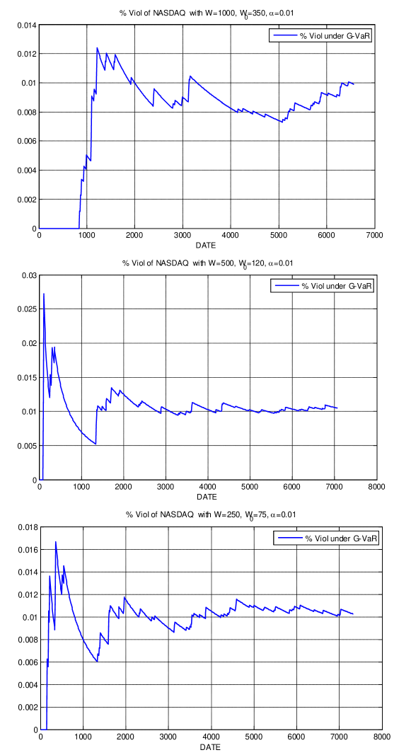
Note that the above percentage is the violation rate of $r_{1,t}$ under the G-VaR model from time $W+1$ to $n+1$, hereafter denoted as %Viol$(n)$.

Figure 2 plots the evolution of %Viol$(n)$ as time $n$ varies. Here, $\alpha=0.01$ is used, but the findings are similar for other values of $\alpha$. For all window sizes $W=1000,500$, and $250$, we find that when $3000\leq n-W$, the violation rate becomes close to the target $\alpha=0.01$. All three cases use a well-calibrated value of $W_{0}=350,~{}120,~{}75$. In practice, as done here for the NASDAQ Index, $W_{0}$ has to be calibrated, and, once fixed, it is kept to forecast future G-VaR values. Condition 5.1 technically guarantees the existence of such a converging window size $W_{0}$. Table 1 presents the summary statistics for the %Viol rates over the converging period $3000<n-W$.

Insert Table 1 around here

Insert Figure 2 around here

To assess the predictive performance of the models under consideration, we follow the test of unconditional coverage, or the binomial test (Kuester et al., 2006). This is in fact a likelihood ratio test for a Bernoulli trial in which the null trial success probability is equal to $\alpha$. More precisely, let $\hat{\alpha}=m_{1}/(m_{0}+m_{1})$ be the sample violation rate %Viol, where $m_{1}$ is the sample number of violations, and the total number of observations is $m_{0}+m_{1}=T-W$. Using the well-known asymptotic $\chi^{2}(1)$ distribution, the $p$-value of the test is

$$\text{LR}_{uc}=P\left(\chi^{2}(1)>2m_{1}\frac{\hat{\alpha}}{\alpha}+2m_{0}\frac{1-\hat{\alpha}}{1-\alpha}\right).$$

Table 2 gives the empirical values of the statistics $\%\text{Viol},\text{LR}_{uc},100\overline{\text{VaR}}$ for the G-VaR with $n=T$, $W=1000$, and $\alpha=0.01,0.025,0.05$. Here, $100\overline{\text{VaR}}$ means $100$ times the average VaR of the related model. The corresponding values of $\%\text{Viol},\text{LR}_{uc},100\overline{\text{VaR}}$ for the AR(1)-GARCH(1,1)-Normal, AR(1)-GARCH(1,1)-Skewed-t, and AR(1)-GARCH(1,1)-Skewed-t-EVT models are directly imported from Table 3 in Kuester et al. (2006). The results in Table 2 show that, for a given $W=1000,\alpha=0.01,0.025,0.05$, once we find the corresponding $W_{0}=350,650,900$, the %Viol of G-VaR is better than that of the AR(1)-GARCH(1,1) model with Normal, Skewed-t, Skewed-t-EVT innovations. See the plot of the $p$-value $\text{LR}_{uc}$ at the bottom of the table. In addition, the values of $100\overline{\text{VaR}}$ in the four models are very close to one another.

Insert Table 2 around here

Kuester et al. (2006) concluded that the AR-GARCH-Skewed-t and AR-GARCH-Skewed-t-EVT VaR models achieve better performance with larger windows, e.g., $W=1000$, than with smaller windows, e.g., $W=500,250$. For G-VaR, however, as suggested by Figure 2, the %Viol statistics are much more stable for $W=500,250$, which suggests better performance with smaller windows. To verify that suggestion, Table 3 gives the empirical statistics of $\%\text{Viol},\text{LR}_{uc},100\overline{\text{VaR}}$ from the G-VaR model for windows $W=500,250$ and risk levels $\alpha$=0.003, 0.005, 0.01, 0.025, 0.05, thereby confirming that G-VaR indeed achieves excellent performance with smaller windows. For the difficult case with the lowest risk level, $\alpha=0.003$, the empirical $p$-value even achieves top values of 0.96 and 1.00!

Insert Table 3 around here

6.2 S&P500 Index

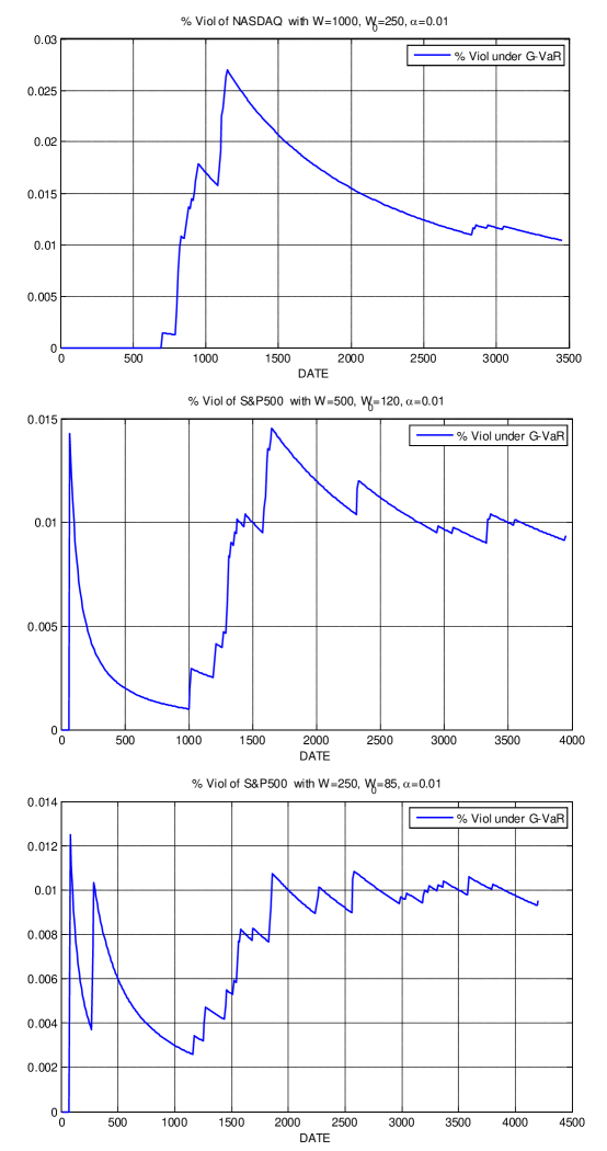
The S&P500 Index data are analyzed using windows $W=1000,500,250$. The window size $W_{0}$ in Condition 5.1 is determined in exactly the same way as for the NASDAQ Composite Index data. Figure 3 replicates Figure 2, but for the S&P500 Index. Summary statistics of %Viol from $3000<n-W$ are given in Table 4 (replicating Table 1, but for the S&P500 Index).

Insert Table 4 around here

Insert Figure 3 around here

Table 5 gives the empirical statistics of $\%\text{Viol},\text{LR}_{uc},100\overline{\text{VaR}}$ for the AR(1)-GARCH(1,1)-Normal, AR(1)-GARCH(1,1)-Skewed-t, AR(1)-GARCH(1,1)-Skewed-t-EVT, and G-VaR models for the S&P500 data with $n=T$, $W=1000$, and $\alpha=0.003,0.005,0.01,0.025,0.05$. These results show that, with a well-calibrated value for $W_{0}$, G-VaR clearly outperforms the three benchmark VaR predictors using AR(1)-GARCH(1,1) filter and Normal, Skewed-t, and Skewed-t-EVT innovations. See the $p$-value plot at the bottom of the table.

The experiments were then repeated for smaller windows, i.e., $W=500$ and 250. The corresponding results for $W=500$ are given in Table 6, with calibrated values $W_{0}=70,110,120,250,480$ for the various risk levels. With the exception of one case, namely, $\alpha=0.05$ with the GARCH-ST-EVT model, G-VaR again outperforms all competitors; see the plot at the bottom of the table. The results for $W=250$ are reported in Table 7. Here, the G-VaR outperforms all competitors uniformly and significantly.

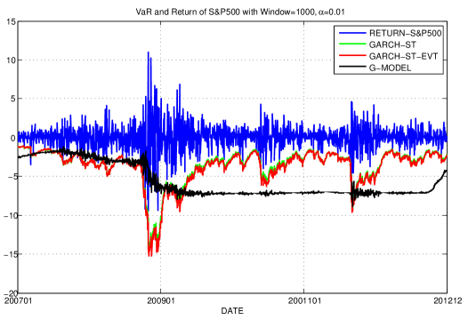
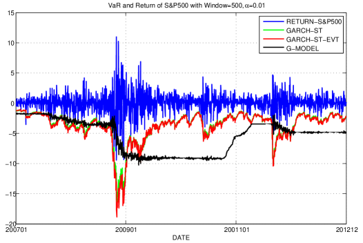
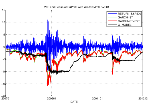
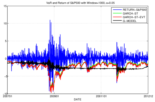
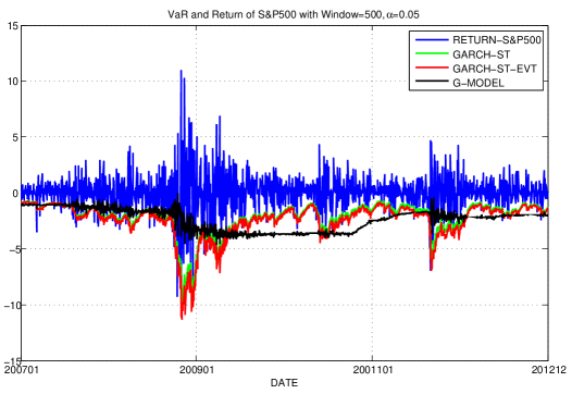
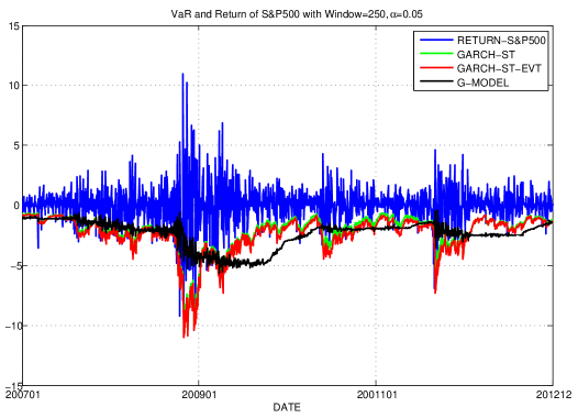
The last plots in Figures 4 and 5 show the time evolution of the three one-step-ahead forecasts given by the G-VaR, AR(1)-GARCH(1,1)-Skewed-t and AR(1)- GARCH(1,1)-Skewed-t-EVT models. Each plot comprises three historical windows, $W=1000,500,250$. The risk level is $\alpha=0.01$ in Figure 4, and $\alpha=0.05$ in Figure 5. All three VaR predictors have the capacity to follow the rise-drop patterns of the original return-series.

Insert Table 5 around here

Insert Table 6 around here

Insert Table 7 around here

Insert Figure 4 around here

Insert Figure 5 around here

6.3 Adaptive window size $W_{0}$

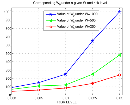
The implementation of G-VaR forecasts requires the existence of an adaptive window $W_{0}$ that enables estimation of the variance parameters $(\underline{\sigma}_{t},\overline{\sigma}_{t})$ of the G-Normal distribution $N(0,[\underline{\sigma}^{2}_{t},\overline{\sigma}^{2}_{t}])$ used at some given time point $t$. Figure 6 displays the values of $W_{0}$ for the different values of $\alpha$ given in Tables 5-7.

$W_{0}$ increases with risk level $\alpha$. As explained earlier (see comments after Condition 5.1), a smaller $\alpha$ implies greater volatility, and a smaller window $W_{0}$ is thus needed under the worst-case scenario adopted in this paper.

Insert Figure 6 around here

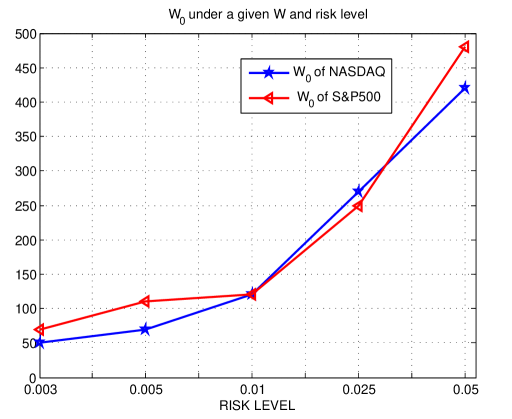
The information carried by these experimental values of $W_{0}$ can be pushed further. In Figure 7, we compare the values found for both the NASDAQ Composite Index and S&P500 Index under different risk levels $\alpha\in\{0.003,0.005,0.01,0.025,0.05\}$, with the historical window size fixed at $W=500$. Because under our worst-case scenario, smaller window sizes $W_{0}$ correspond to higher volatility (and thus higher risk in the index), we can assume that the S&P500 Index return is riskier than the NASDAQ Composite Index return at risk level $\alpha=0.025$. Their degree of risk is comparable at risk level $\alpha=0.01$, and the S&P500 Index is probably less risky at risk levels $\alpha=0.003,0.005$, and 0.05.

Insert Figure 7 around here

Finally, note that we used an initial segment of 3000 data points to determine the parameter $W_{0}$ in both cases of the NASDAQ Composite Index and S&P 500 Index. Once $W_{0}$ is found, it is kept fixed and used for different moving windows $W=1000,500,250$. Therefore, the G-VaR forecasts can be considered as in-sample forecasts for initial $3000+W$ data points, while they are out-sample ones for the remaining $n-(3000+W)$ data points.

7 Discussion

This paper introduces a new VaR predictor, G-VaR, for financial return series. Our methodology is based on the model-uncertainty principle that the volatility of returns cannot be adequately characterized by a single statistical distribution or model. Rather, an infinite family of distributions is necessary for full characterization. Considering the worst-case volatility scenario among these numerous potential distributions, and using the recent theory of SLE, we formally identity G-VaR through a new mathematical object called $G$-normal distribution. Extensive empirical analysis using the NASDAQ Composite Index and S&P500 Index shows the G-VaR predictor to outperform many of the existing benchmark predictors of VaR. Its superiority is particularly significant for low risk levels, such as $\alpha=1\%$ or 0.5%.

It is difficult to provide a completely clear explanation for the surprising success of G-VaR. Most likely, the concept of model uncertainty has particular strength when considering the volatility of returns. Such volatility is time-varying, and is reputed to be complex in nature, and thus the worst-case scenario approach taken by G-VaR over all potential volatility distributions proves to be an excellent fit to the analysed data. Judged by the empirical results presented herein, this model-uncertainty approach appears more powerful than many of the existing approaches with model certainty, wherein a unique statistical distribution is assumed for the volatility process.

However, a number of unanswered question remain to be investigated in future. In particular, the implementation of G-VaR depends on an adaptive window $W_{0}$. Although it has been shown that this “tuning parameter” can be efficiently determined empirically for the two datasets analyzed in this paper, it would be worth investigating more its intrinsic or physical meaning. It would also be valuable to analyze the performance of the G-VaR predictor on other financial series to determine the extent to which the worst-case scenario approach under model uncertainty remains successful. More generally, it would be useful to explore other financial or even non-financial datasets in which model uncertainty is unavoidable. The SLE theory could also provide new data analytic tools in the vein of the G-VaR approach developed in this paper for the volatility of returns.

Appendix A Relevant results from sublinear expectations

In this appendix, we introduce the relevant concepts and properties of the general theory of sublinear expectation used in the paper. Let $\Omega$ be an arbitrarily given set and $\mathcal{H}$ be a linear space of real functions, called random variables, defined on $\Omega$ such that, if $\xi\in\mathcal{H}$, then $\left|\xi\right|\in\mathcal{H}$. We also assume that $1\in\mathcal{H}$. The space $\mathcal{H}$ is called a vector lattice on $\Omega$. We make the following assumption: if $\xi_{1},\cdots,\xi_{n}\in\mathcal{H}$, or equivalently, $\xi=(\xi_{1},\cdots,\xi_{n})\in\mathcal{H}^{n}$, then $\phi(\xi)\in\mathcal{H}$ for each function $\phi$ in $C_{l.Lip}(\mathbb{R}^{n})$. Here, $\phi$ corresponds to some characteristic of $\xi$, and $C_{l.Lip}(\mathbb{R}^{n})$ is the space of all functions $\phi$ defined on $\mathbb{R}^{n}$ satisfying

$$\left|\phi(x)-\phi(y)\right|\leq C(1+\left|x\right|^{m}+\left|y\right|^{m})\left|x-y\right|,\quad x,y\in\mathbb{R}^{n},$$

for some $C>0$ and $m\in\mathbb{N}$ depending on $\phi$. Similarly, with the probability space, we introduce a sublinear expectation $\mathbb{E}$ on $\mathcal{H}$ that was first proposed in Peng (2006).

Definition A.1.

A function $\mathbb{E}:\mathcal{H}\to\mathbb{R}$ is called a sublinear expectation on $(\Omega,\mathcal{H})$ if it satisfies

1). Monotonicity: if $X(\omega)\geq Y(\omega)$ for each $\omega\in\Omega$, then $\mathbb{E}[X]\geq\mathbb{E}[Y]$;

2). $\mathbb{E}[X+c]=\mathbb{E}[X]+c$ for any $c\in\mathbb{R}$;

3). $\mathbb{E}[X+Y]\leq\mathbb{E}[X]+\mathbb{E}[Y]$; and

4). $\mathbb{E}[\lambda X]=\lambda\mathbb{E}[X]$ for any $\lambda\geq 0$.

A closely associated concept is coherent risk measures introduced in Artzner et al. (1999). From a mathematical point of view, this concept essentially coincides with that of sublinear expectation. What makes the difference is perhaps the respective contexts where the two concepts are introduced and used. Coherent risk measures are introduced within mathematical finance (or financial mathematics) and dedicated to study problems and subjects in this area, for example market risks and non-market risks. On the other hand, sublinear expectation is more abstract and introduced within general probability theory. For example, objects and concepts like Brownian motion, conditional expectation and martingale have been developed under sublinear expectation. A related discussion is Denis et al. (2011) where a representation theorem of a coherent risk measure is proposed.

Let $X_{1}$ and $X_{2}$ be two $n$-dimensional random vectors defined on nonlinear expectation spaces $(\Omega_{1},\mathcal{H}_{1},\mathbb{E}_{1})$ and $(\Omega_{2},\mathcal{H}_{2},\mathbb{E}_{2})$, respectively. They are called identically distributed, denoted by $X_{1}:\overset{d}{=}X_{2}$, if

$$\mathbb{E}_{1}[\phi(X_{1})]=\mathbb{E}_{2}[\phi(X_{2})],\quad\forall\phi\in C_{l.Lip}(\mathbb{R}^{n}).$$

A random vector $Y\in\mathcal{H}^{n}$ is said to be independent of $X\in\mathcal{H}^{m}$ if, for each $\phi\in C_{l.Lip}(\mathbb{R}^{m}\times\mathbb{R}^{n})$, we have

$$\mathbb{E}[\phi(X,Y)]=\mathbb{E}[\mathbb{E}[\phi(x,Y)]_{x=X}].$$

If the above equality holds only for a specific $\phi$, then we say that $Y$ is uncorrelated to $X$ with respect to this function $\phi$. Under a sublinear expectation $\mathbb{E}$, the independence of $Y$ from $X$ means that the uncertainty of distributions of $Y$ does not change with each realization of $X(\omega)=x,\ x\in\mathbb{R}^{n}$. It is important to note that this independence under sublinear expectation is not symmetric; in particular “$Y$ is independent of $X$” is not equivalent to “$X$ is independent of $Y$.” For illustration we consider an example that generalizes the one in Peng (2019).

Example A.1.

Let $\xi,X,Y,Z\in\mathcal{H}$ be identically distributed satisfying $\mathbb{E}[\xi]=\mathbb{E}[-\xi]=0$ and ${\overline{\sigma}}^{2}=\mathbb{E}[\xi^{2}]>{\underline{\sigma}}^{2}=-\mathbb{E}[-\xi^{2}]$. We suppose $\mathbb{E}[\left|\xi\right|]=\mathbb{E}[\xi^{+}+\xi^{-}]>0$, thus

$$\mathbb{E}[\xi^{+}]=\frac{1}{2}\mathbb{E}[\left|\xi\right|+\xi]=\frac{1}{2}\mathbb{E}[\left|\xi\right|]>0,$$

and

$$\mathbb{E}[\xi^{-}]=\frac{1}{2}\mathbb{E}[\left|\xi\right|-\xi]=\frac{1}{2}\mathbb{E}[\left|\xi\right|]>0.$$

Assume that $Z$ is independent of $\{X,Y\}$ and $Y$ is independent of $X$, we can show that

$$\mathbb{E}[XY]=0,\ \mathbb{E}[\left|XY\right|]=(\mathbb{E}[\left|X\right|])^{2}>0,\ \mathbb{E}[(XY)^{+}]=\mathbb{E}[(XY)^{-}]=\frac{1}{2}\mathbb{E}[\left|XY\right|]>0,$$

and

$$\mathbb{E}[XYZ^{2}]=\mathbb{E}[(XY)^{+}{\overline{\sigma}}^{2}-(XY)^{-}{\underline{\sigma}}^{2}]=({\overline{\sigma}}^{2}-{\underline{\sigma}}^{2})\mathbb{E}[(XY)^{+}]>0.$$

In contrast, if we assume that $X$ is independent of $Y$ and $\{X,Y\}$ are independent of $Z$, we have

$$\mathbb{E}[XYZ^{2}]=\mathbb{E}[\mathbb{E}[XYz^{2}]_{z=Z}]=\mathbb{E}[Z^{2}]\mathbb{E}[XY]=0.$$

Therefore, by reversing the order of independence, we obtain different values for $\mathbb{E}[XYZ^{2}]$. This shows the asymmetry of the concept of independence under sublinear expectation while the concept is symmetric in classical probability theory.

Finally, further properties of the G-normal distribution are rigorously established as follows.

Proposition A.1.

The solution of the fully nonlinear PDE (3.3) with Cauchy initial condition (4.5) has the following explicit expression;

$$u(t,x)=\int_{-\infty}^{x}\rho(t,y)dy,$$

where $\rho(t,y)$ is a function on $\mathbb{R_{+}}\times\mathbb{R}$ defined by

$$\rho(t,y)=\frac{\sqrt{2}}{(\overline{\sigma}+\underline{\sigma})\sqrt{\pi t}}\left[e^{-\frac{y^{2}}{2\overline{\sigma}^{2}t}}I(y\leq 0)+e^{-\frac{y^{2}}{2\underline{\sigma}^{2}t}}I(y>0)\right].$$

Proof.

Using classical analysis of the heat equation, we can prove that $\displaystyle\lim_{t\to 0}u(t,x)=1_{(0,\infty)}(x)$ for each $x$. If $x<0$, we have $\rho(t,x)=\frac{\sqrt{2}}{(\overline{\sigma}+\underline{\sigma})\sqrt{\pi t}}e^{-\frac{x^{2}}{2\overline{\sigma}^{2}t}}$ and can obtain that

$$\partial_{t}u(t,x)=\partial_{x}\rho(t,x)=\frac{-x}{(\overline{\sigma}+\underline{\sigma})\sqrt{2\pi t^{3}}}e^{-\frac{x^{2}}{2\overline{\sigma}^{2}t}},$$ (A.1)

$$\partial_{x}u(t,x)=\rho(t,x)=\frac{\sqrt{2}}{(\overline{\sigma}+\underline{\sigma})\sqrt{\pi t}}e^{-\frac{x^{2}}{2\overline{\sigma}^{2}t}},$$

$$\partial_{xx}^{2}u(t,x)=\partial_{x}\rho(t,x)=\frac{-\sqrt{2}x}{(\overline{\sigma}+\underline{\sigma}){\overline{\sigma}}^{2}\sqrt{\pi t^{3}}}e^{-\frac{x^{2}}{2\overline{\sigma}^{2}t}}.$$

Thus, we can verify

$$\partial_{t}u(t,x)-G(\partial_{xx}^{2}u(t,x))=0,\ x<0,t>0.$$

In a similar manner, we have

$$\partial_{t}u(t,x)-G(\partial_{xx}^{2}u(t,x))=0,\ x<0,t>0.$$

Note that $\partial_{xx}^{2}u(t,x)$ is continuous on $(0,\infty)\times\mathbb{R}$, and $\partial_{xx}^{2}u(t,0)=0,\partial_{t}u(t,0)=0$, thus, one obtains,

$$\partial_{t}u(t,x)-G(\partial_{xx}^{2}u(t,x))=0,\ x=0,t>0.$$

Consequently, $u(t,x)$ solves the PDE (3.3) on the entire $(0,\infty)\times\mathbb{R}$ in the sense of classical solution. ∎

Figure 1: Density of one distribution of G-normal distribution with variance parameters $(\underline{\sigma},\overline{\sigma})=(0.5,1)$ in comparison with standard normal density.

Figure 2: NASDAQ Composite Index: convergence of the violation rate %Viol for $W=1000,500,250$, and $\alpha=0.01$. The adaptive window sizes are $W_{0}=350,120,75$, respectively.

Figure 3: S&P500 Index: convergence of the violation rate %Viol for $W=1000,500,250$, and $\alpha=0.01$. These adaptive window sizes are $W_{0}=250,120,85$, respectively.

Figure 4: For a given $W=1000,500,250$, the VaR performance of different models at risk level $\alpha=0.01$..

Figure 5: For a given $W=1000,500,250$, the VaR performance of different models at risk level $\alpha=0.05$.

Figure 6: S&P 500 Index data: variation of adaptive window $W_{0}$ for different risk levels $\alpha$ and historical windows $W$.

Figure 7: For a given $W=500,\alpha=0.003,0.005,0.01,0.025,0.05$, $W_{0}$ of NASDAQ and S&P500 indexes.

Table 1: NASDAQ Composite Index: Average and standard deviations of %Viol with $W$=1000, 500, 250 and $\alpha=0.01$.

Model	Window $W$	Window $W_{0}$	Average value	Standard deviation
G-VaR:	1000	350	0.0087	8.1160e-04
	500	120	0.0103	3.9274e-04
	250	75	0.0104	5.9560e-04

Table 2: NASDAQ Composite Index: Empirical statistics of G-VaR forecast compared with forecasts of three benchmark predictors reported in Kuester et al. (2006) with $W$=1000. The bottom plot shows the $\text{LR}_{uc}$, where $\text{LR}_{uc}$ is the p-values of the Binomial test.

Model	100$\alpha$	%Viol.	$\text{LR}_{uc}$	$100\overline{\text{VaR}}$
AR(1)-GARCH(1,1)-N: $\left\{\begin{tabular}[]{@{}c@{}}\\ \\ \\ \end{tabular}\right.$	1 2.5 5	2.23 3.92 6.21	0.00 0.00 0.00	2.05 1.72 1.43
AR(1)-GARCH(1,1)-St: $\left\{\begin{tabular}[]{@{}c@{}}\\ \\ \\ \end{tabular}\right.$	1 2.5 5	1.2 2.72 5.12	0.12 0.25 0.65	2.57 2.01 1.59
AR(1)-GARCH(1,1)-St-EVT: $\left\{\begin{tabular}[]{@{}c@{}}\\ \\ \\ \end{tabular}\right.$	1 2.5 5	0.97 2.47 5.06	0.82 0.87 0.82	2.70 2.07 1.61
G-VaR: $W_{0}$=$\left\{\begin{tabular}[]{@{}c@{}}350\\ 650\\ 900\end{tabular}\right.$	1 2.5 5	0.99 2.51 5.03	0.93 0.96 0.90	2.78 2.06 1.52

Table 3: NASDAQ Composite Index with W=500, 250

Model	100$\alpha$	%Viol.	$\text{LR}_{uc}$	$100\overline{\text{VaR}}$
$W$=500: $W_{0}$=$\left\{\begin{tabular}[]{@{}c@{}}50\\ 70\\ 120\\ 270\\ 420\end{tabular}\right.$	0.3 0.5 1 2.5 5	0.30 0.49 1.05 2.54 5.00	0.96 0.95 0.70 0.81 0.99	4.71 4.00 3.11 2.14 1.60
$W$=250: $W_{0}$=$\left\{\begin{tabular}[]{@{}c@{}}35\\ 50\\ 75\\ 150\\ 210\end{tabular}\right.$	0.3 0.5 1 2.5 5	0.30 0.52 1.02 2.49 5.05	1.00 0.82 0.84 0.93 0.84	4.29 3.67 2.98 2.12 1.61

Table 4: S&P500 Index: Average and standard deviations of %Viol with $W$=1000, 500, 250 and $\alpha=0.01$

Model	Window $W$	Window $W_{0}$	Average value	Standard deviation
G-VaR:	1000	250	0.0111	4.1705e-04
	500	120	0.0097	3.6689e-04
	250	85	0.0099	3.0967e-04

Table 5: S&P 500 Index: Empirical statistics of VaR forecasts from G-VaR and three benchmark predictors with $W$=1000. The bottom plot shows the $\text{LR}_{uc}$.

Model	100$\alpha$	%Viol.	$\text{LR}_{uc}$	$100\overline{\text{VaR}}$
AR(1)-GARCH(1,1)-N: $\left\{\begin{tabular}[]{@{}c@{}}\\ \\ \\ \\ \\ \end{tabular}\right.$	0.3 0.5 1 2.5 5	1.15 1.55 2.42 3.83 6.08	0.00 0.00 0.00 0.00 0.00	2.64 2.47 2.23 1.87 1.56
AR(1)-GARCH(1,1)-St: $\left\{\begin{tabular}[]{@{}c@{}}\\ \\ \\ \\ \\ \end{tabular}\right.$	0.3 0.5 1 2.5 5	0.28 0.73 1.32 3.24 5.71	0.83 0.07 0.07 0.01 0.06	3.42 3.06 2.61 2.03 1.60
AR(1)-GARCH(1,1)-St-EVT: $\left\{\begin{tabular}[]{@{}c@{}}\\ \\ \\ \\ \\ \end{tabular}\right.$	0.3 0.5 1 2.5 5	0.39 0.62 1.21 2.79 4.73	0.33 0.33 0.33 0.28 0.45	3.38 3.10 2.70 2.16 1.72
G-VaR: $W_{0}$=$\left\{\begin{tabular}[]{@{}c@{}}90\\ 150\\ 250\\ 650\\ 1000\end{tabular}\right.$	0.3 0.5 1 2.5 5	0.29 0.52 1.07 2.49 4.87	0.91 0.86 0.68 0.97 0.72	7.05 5.77 4.40 2.91 1.94

Table 6: S&P 500 Index: Empirical statistics of VaR forecasts from G-VaR and three benchmark predictors with $W$=500. The bottom plot shows the $\text{LR}_{uc}$.

Model	100$\alpha$	%Viol.	$\text{LR}_{uc}$	$100\overline{\text{VaR}}$
AR(1)-GARCH(1,1)-N: $\left\{\begin{tabular}[]{@{}c@{}}\\ \\ \\ \\ \\ \end{tabular}\right.$	0.3 0.5 1 2.5 5	1.06 1.38 2.22 3.82 5.90	0.00 0.00 0.00 0.00 0.01	2.75 2.58 2.32 1.95 1.63
AR(1)-GARCH(1,1)-St: $\left\{\begin{tabular}[]{@{}c@{}}\\ \\ \\ \\ \\ \end{tabular}\right.$	0.3 0.5 1 2.5 5	0.27 0.59 1.18 3.13 5.67	0.74 0.42 0.25 0.01 0.05	3.51 3.16 2.69 2.11 1.67
AR(1)-GARCH(1,1)-St-EVT: $\left\{\begin{tabular}[]{@{}c@{}}\\ \\ \\ \\ \\ \end{tabular}\right.$	0.3 0.5 1 2.5 5	0.37 0.62 1.06 2.57 5.01	0.43 0.31 0.70 0.79 0.98	3.44 3.16 2.77 2.23 1.80
G-VaR: $W_{0}$=$\left\{\begin{tabular}[]{@{}c@{}}70\\ 110\\ 120\\ 250\\ 480\end{tabular}\right.$	0.3 0.5 1 2.5 5	0.33 0.51 0.96 2.48 5.08	0.74 0.96 0.81 0.90 0.81	5.50 4.58 4.08 2.79 1.90

Table 7: S&P 500 Index: Empirical statistics of VaR forecasts from G-VaR and three benchmark predictors with $W$=250. The bottom plot shows the $\text{LR}_{uc}$.

Model	100$\alpha$	%Viol.	$\text{LR}_{uc}$	$100\overline{\text{VaR}}$
AR(1)-GARCH(1,1)-N: $\left\{\begin{tabular}[]{@{}c@{}}\\ \\ \\ \\ \\ \end{tabular}\right.$	0.3 0.5 1 2.5 5	1.30 1.72 2.56 4.09 6.23	0.00 0.00 0.00 0.00 0.00	2.78 2.61 2.35 1.97 1.65
AR(1)-GARCH(1,1)-St: $\left\{\begin{tabular}[]{@{}c@{}}\\ \\ \\ \\ \\ \end{tabular}\right.$	0.3 0.5 1 2.5 5	0.40 0.70 1.39 3.3 5.95	0.28 0.08 0.01 0.00 0.01	3.47 3.13 2.68 2.12 1.69
AR(1)-GARCH(1,1)-St-EVT: $\left\{\begin{tabular}[]{@{}c@{}}\\ \\ \\ \\ \\ \end{tabular}\right.$	0.3 0.5 1 2.5 5	0.65 0.86 1.40 2.90 5.18	0.00 0.00 0.01 0.10 0.59	3.32 3.06 2.71 2.22 1.80
G-VaR: $W_{0}$=$\left\{\begin{tabular}[]{@{}c@{}}45\\ 60\\ 85\\ 140\\ 240\end{tabular}\right.$	0.3 0.5 1 2.5 5	0.29 0.48 0.98 2.55 4.95	0.86 0.82 0.87 0.85 0.88	4.73 4.16 3.46 2.57 1.83

References

- Abad et al. (2014) P. Abad, S. Benito, and C. Lipez. A comprehensive review of value at risk methodologies. The Spanish Review of Financial Economics, 12(1):15–32, 2014. ISSN 2173-1268.
- Artzner et al. (1999) P. Artzner, F. Delbaen, J.-M. Eber, and D. Heath. Coherent measures of risk. Mathematical Finance, 9:203–228, 1999.
- Avellaneda et al. (1995) M. Avellaneda, A. Levy, and A. Parás. Pricing and hedging derivative securities in markets with uncertain volatilities. Applied Mathematical Finance, 2:73–88, 1995.
- Barone-Adesi et al. (1999) G. Barone-Adesi, K. Giannopoulos, and L. Vosper. VaR without correlations for portfolios of derivative securities. Journal of Futures Markets, 19:583–602, 1999.
- Barone-Adesi et al. (2002) G. Barone-Adesi, K. Giannopoulos, and L. Vosper. Backtesting derivative portfolios with Filtered Historical Simulation (FHS). European Financial Management, 8:31–58, 2002.
- Bollerslev (1986) T. Bollerslev. Generalized autoregressive conditional heteroskedasticity. Journal of Econometrics, 31:307–327, 1986.
- Chen and Epstein (2002) Z. Chen and L. Epstein. Ambiguity, risk, and asset returns in continuous time. Econometrica, 70(4):1403–1443, 2002.
- Chernozhukov and Umantsev (2001) V. Chernozhukov and L. Umantsev. Conditional value-at-risk: Aspects of modeling and estimation. Empirical Economics, 26(1):271–292, 2001.
- Christoffersen (2003) P. F. Christoffersen. Elements of Financial Risk Management. Academic Press, Amsterdam, 2003.
- Cont (2006) R. Cont. Model uncertainty and its impact on the pricing of derivative instruments. Mathematical Finance, 16:519–547, 2006.
- Denis et al. (2011) L. Denis, M. Hu, and Peng. S. Function spaces and capacity related to a sublinear expectation: application to G-Brownian motion paths. Potential Analysis, 34:139–161, 2011.
- Dowd (2002) K. Dowd. Measuring Market Risk. John Wiley & Sons, Chichester, 2002.
- Embrechts et al. (1997) P. Embrechts, K. Klüppelberg, and T. Mikosch. Modelling Extremal Events for Insurance and Finance. Springer, Berlin, 1997.
- Engle and Manganelli (2004) R.F. Engle and S. Manganelli. CAViaR: Conditional autoregressive value at risk by regression quantiles. Journal of Business and Economic Statistics, 22(4):367–381, 2004.
- Epstein and Ji (2013) L. G. Epstein and S. Ji. Ambiguous volatility and asset pricing in continuous time. Review of Financial Studies, 26(7):1740–1786, 2013.
- Fang et al. (2019) X. Fang, S. Peng, Q. Shao, and Y. Song. Limit theorems with rate of convergence under sublinear expectations. Bernoulli, 25:1–31, 2019.
- Föllmer and Schied (2011) H. Föllmer and A. Schied. Stochastic Finance. An Introduction in Discrete Time. Third revised and extended edition. Walter de Gruyter & Co., Berlin, 2011.
- Gospodinov and Maasoumi (2018) N. Gospodinov and E. Maasoumi. Generalized aggregation of misspecified models: with an application to asset pricing. Technical report, https://sites.google.com/site/gospodinovfed/, 2018.
- Haas et al. (2004) M. Haas, S. Mittnik, and M. S. Paolella. Mixed normal conditional heteroskedasticity. Journal of Financial Econometrics, 2:211–250, 2004.
- Huber (1981) P. J. Huber. Robust Statistics. Wiley Series in Probability and Mathematical Statistics. John Wiley & Sons, Inc., New York, 3rd edition, 1981.
- Jin and Peng (2016) H. Jin and S. Peng. Optimal unbiased estimation for maximal distribution. arXiv:1611.07994v1, 2016.
- Jorion (2007) Ph. Jorion. Value at Risk : the New Benchmark for Managing Financial Risk. McGraw-Hill, New York, 3rd edition, 2007.
- Jorion (2010) Ph. Jorion. Risk management. Annual Review of Financial Economics, 2(1):347–365, 2010.
- Kerkhof et al. (2010) J. Kerkhof, B. Melenberg, and H. Schumacher. Model risk and capital reserves. Journal of Banking & Finance, 34:267–279, 2010.
- Koenker and Bassett (1978) R. Koenker and G. Bassett. Regression quantiles. Econometrica, 46:33–50, 1978.
- Kuester et al. (2006) K. Kuester, S. Mittnik, and M. S. Paolella. Value-at-Risk Prediction: A comparison of alternative strategies. Journal of Financial Econometrics, 4(1):53–89, 2006.
- Lyons (1995) T. J. Lyons. Uncertain volatility and the risk-free synthesis of derivatives. Applied Mathematical Finance, 2:117–133, 1995.
- McNeil and Frey (2000) A. J. McNeil and R. Frey. Estimation of tail-related risk measures for heteroscedastic financial time series: An extreme value approach. Journal of Empirical Finance, 7:271–300, 2000.
- Nadarajah and Chan (2016) S. Nadarajah and S. Chan. Estimation methods for value at risk. In Extreme Events in Finance: A Handbook of Extreme Value Theory and its Applications, pages 283–356. Wiley, 2016. ISBN 9781118650318.
- Peng (1997) S. Peng. Backward SDE and related g-expectation. Backward stochastic differential equations (Paris, 1995-1996) 141-159. Pitman Res. Notes Math. Ser., Longman, Harlow, 1997.
- Peng (2004) S. Peng. Filtration consistent nonlinear expectations and evaluations of contingent claims. Acta Mathematicae Applicatae Sinica, 20:1–24, 2004.
- Peng (2006) S. Peng. Stochastic Analysis and Applications: The Abel Symposium 2005, chapter ”-expectation, -Brownian motion and related stochastic calculus of Itô type”. Springer, Berlin Heidelberg, 2006.
- Peng (2008) S. Peng. Multi-dimensional G-Brownian motion and related stochastic calculus under G-expectation. Stochastic Processes and Their Applications, 118:2223–2253, 2008.
- Peng (2017) S. Peng. Theory, methods and meaning of nonlinear expectation theory. Scientia Sinica Mathematica: In Chinese, 47:1223–1254, 2017.
- Peng (2019) S. Peng. Nonlinear Expectations and Stochastic Calculus under Uncertainty. Springer, Berlin, Heidelberg, 2019.
- Pickands (1975) J. Pickands. Statistical inference using extreme order statistics. Annals of Statistics, 3:119–131, 1975.
- Walley (1991) P. Walley. Statistical reasoning with imprecise probabilities. Monographs on Statistics and Applied Probability, 42. Chapman and Hall, Ltd., London, 1991.
- Zhang and Nadarajah (2017) Y. Zhang and S. Nadarajah. A review of backtesting for value at risk. Communications in Statistics - Theory and Methods, pages 1–24, 2017.