On Arbitrarily Long Periodic Orbits of Evolutionary Games on Graphs

Abstract.

A periodic behavior is a well observed phenomena in biological and economical systems. We show that evolutionary games on graphs with imitation dynamics can display periodic behavior for an arbitrary choice of game theoretical parameters describing social-dilemma games. We construct graphs and corresponding initial conditions whose trajectories are periodic with an arbitrary minimal period length. We also examine a periodic behavior of evolutionary games on graphs with the underlying graph being an acyclic (tree) graph. Astonishingly, even this acyclic structure allows for arbitrary long periodic behavior.

Jeremias Epperlein^∗

Center for Dynamics & Institute for Analysis

Dept. of Mathematics

Technische Universität Dresden, 01062

Dresden, Germany

Vladimír Švígler

Department of Mathematics and NTIS

Faculty of Applied Sciences

University of West Bohemia

Univerzitní 8, 30614

Pilsen, Czech Republic

1. Introduction

Evolutionary game theory on graphs in the spirit of Nowak and May [13] studies the evolution of social behavior in spatially structured populations. In our setting, each vertex of a graph is assigned a strategy. In every time step, each vertex plays a matrix game with its imminent neighbors. The resulting game utilities together with the update order (certain vertices can remain rigid) and the update function result in the change of strategy to the subsequent time step. Here, we focus on the case of synchronous update order and deterministic imitation dynamics - every vertex copies the strategy of the most successful neighbor including itself. From a biological point of view, it is natural to consider a stochastic update rule leading mathematically to a Markov chain. This is also the approach taken by most rigorous investigations of such systems, see for example [4] and [2]. Randomness can also be used to introduce mutations of the individuals into the model, see for example [2]. However, questions about the dynamical behavior of these models often become intractable because of the stochastic nature of the system. Different authors therefore also studied deterministic versions of the model, see for example [1, 5, 9, 11, 13, 14]. The results regarding this deterministic version, however, are almost all obtained by simulations.

One of the factors influencing dynamics heavily are the parameters of the underlying matrix game. We consider a two strategy game (Cooperation, Defection) whose interpretation leads to a natural division of the parameter space into $4$ scenarios Prisoner’s dilemma, Stag hunt, Hawk and dove, Full cooperation. The equilibria of the replicator dynamics based on matrix games with such parameters are already well known, [8].

In [13] it was shown by simulations that even on lattices these dynamical systems can show very complicated behavior starting from a very simple initial condition, see also Chapter 9 in [12]. Nowak and May show for example that the systems can exhibit cascading behavior. Most of the time, such constructions work for very specific choices of parameters.

Our main questions is thus: Can arbitrarily long periodic behavior happen for all parameter choices? For example, the replicator dynamics with parameters of HD scenario tend to a stable mixed equilibrium but only pure equilibria are attractive for the other scenarios. The spatial structure of the game must be thus thoroughly examined. We will answer the question positively by explicitly constructing the graphs demonstrating the required behavior for each set of parameters.

In this paper, we focus on evolutionary games on a graph with periodic trajectories along which the strategy profiles (number of cooperators and defectors) change. Periodic behavior with no change in the strategy profiles was observed for example in [12] by Nowak and May in a structure they called a walker (spaceship in cellular automata terms). Moreover, such a structure is automorphism invariant in a certain sense; for each time step, there exists a graph automorphism which keeps the moving walker in one place. Such structures may be of interest for future research. We note, that our constructions introduce a periodic behavior of arbitrary length both in strategy vectors (distribution of strategies) and strategy profiles.

Evolutionary games on graphs also form a very interesting class of cellular automata. Cellular automata on a lattice can take into account the relative spatial position of a neighbor. The dependence on the neighbor on the left might differ from the dependence on the neighbor on the right. On an arbitrary graph this is only possible if the edges carry some kind of label. A cellular automaton in which the new state of a cell depends only on its own state and the number of neighboring cells in each state is called totalistic. Such cellular automata are naturally defined also on unlabeled graphs. While evolutionary games as considered here are not totalistic, they nevertheless are defined on unlabeled graphs in an obvious way. See [10] for a discussion of cellular automata on graphs.

The paper is organized as follows. We introduce basic notation and the dynamics of evolutionary games on a graph in Section 2. In Section 3, Theorem 3.1, answering the main question of this paper, is stated and proved. The proof is carried out for two separate cases depending on the parameter scenario. Periodic behavior of evolutionary games on a graph with the underlying graph being a tree is examined in Section 4. We conclude our results in Section 5.

2. Preliminaries

We are considering undirected connected graphs $\mathcal{G}$ as the spatial structure of our game with the vertices $V$ being players. The interactions between vertices are defined by a set of edges $E$ (no edge means no direct interaction). The $m$-neighborhood of the vertex $i$ (the set of all vertices having distance to $i$ exactly $m$) is denoted by $N_{m}(i)$. We also define

$$N_{\leq m}(v):=\bigcup_{n=1}^{m}N_{n}(v)\cup\{v\}.$$

The strategy set of the game is simply $S=\{\text{"Cooperate"},\text{"Defect"}\}=\{C,D\}=\{1,0\}$. The neighboring vertices play a matrix game where the resulting utilities are defined by the matrix

$$\begin{array}[]{c|cc}&C&D\\ \hline\cr C&a&b\\ D&c&d\end{array}$$

and the utility function $u$. For example, if player A cooperates and player B defects, player A gets utility b and player B gets utility c. In each time step, a certain subset of players is allowed to change their strategy based on the update order $\mathcal{T}$. Finally, the strategy update is defined by a function $\varphi$. A general framework of evolutionary games on graphs was developed in [7]. An evolutionary game on a graph can be formally defined as follows.

Definition 2.1.

An evolutionary game on a graph is a quintuple $(\mathcal{G},\pi,u,\mathcal{T},\varphi)$, where

1. $\mathcal{G}=(V,E)$ is a connected graph,

2. $\pi=(a,b,c,d)$ are game-theoretical parameters,

3. $u:S^{V}\to\mathbb{R}^{V}$ is a utility function,

4. $\mathcal{T}:\mathbb{N}_{0}\to 2^{V}$ is an update order,

5. $\varphi:(\mathbb{N}_{0})^{2}_{\geq}\times S^{V}\to S^{V}$ is a dynamical system.

The strategy vector (the state of the system) will be denoted $X=(x_{1},\ldots,x_{|V|})\in S^{V}$. For a strategy vector $X\in S^{V}$, the strategy of the vertex $v$ is $X_{v}$. The utility of a player $v$ is given by $u_{v}(X)$.

Our main focus lies in social dilemma games and we are thus interested in the game-theoretical parameters $\mathcal{P}$ describing such games. In particular, it is more advantageous if the opponent cooperates than if it defects for each player, i.e.

$$\min\{a,c\}>\max\{b,d\}\,.$$

This results into four possible scenarios: Prisoner’s dilemma (PD): $c>a>d>b$, Stag hunt (SH): $a>c>d>b$, Hawk and dove (HD): $c>a>b>d$ and Full cooperation (FC): $a>c>b>d$. Demanding the inequalities to be strict only excludes sets of measure zero. This generic payoff assumption is common in examining game-theoretical models (see e.g. [3]). From now on, we consider the mean utility function

$$u_{i}(X)=\frac{1}{|N_{1}(i)|}\left(a\sum_{j\in N_{1}(i)}X_{i}X_{j}+b\sum_{j\in N_{1}(i)}X_{i}(1-X_{j})+\right.\\ \left.+c\sum_{j\in N_{1}(i)}(1-X_{i})X_{j}+d\sum_{j\in N_{1}(i)}(1-X_{i})(1-X_{j})\right)$$

which is an averaged sum of the outcomes of the matrix games played with direct neighbors. Without loss of generality, we can now assume $a=1,d=0$ and thus the parameter regions can be depicted in the plane (see Figure 1).

Figure 1. Regions of admissible parameters $\mathcal{P}$ with normalization $a=1,d=0$.

This simplification can be done thanks to the averaging property of the mean utility function (see [6, Remark 8.]). In Question 1, Theorem 3.1 and Theorem 4.1 we assume a synchronous update order only, i.e. $\mathcal{T}(t)=V$ for all $t\in\mathbb{N}_{0}$. In other words, all vertices are updated simultaneously at every time step. However, the definitions from Section 2 make sense for an arbitrary update order. Finally, the dynamical system $\varphi$ follows the deterministic imitation dynamics; namely, each vertex adopts the strategy of its most successful neighbor (including itself). Formally,

$$\varphi_{i}(t+1,t,X)=\left\{\begin{array}[]{ll}X_{\text{max}}&i\in\mathcal{T}(t),\;|A_{i}(X)|=1\;\text{and}\;A_{i}(X)=\left\{X_{\text{max}}\right\}\,,\\ X_{i}&\text{otherwise}\,,\end{array}\right.$$

where

$$A_{i}(x)=\left\{X_{k}\,|\,k\in\text{argmax}\left\{u_{j}(X)\,|\,j\in N_{1}(i)\cup\{i\}\right\}\right\}\,.$$

We refer to [6] for further discussion on the utility function, update order and the dynamics.

Considering a deterministic dynamical system, the natural interest lies in examining the existence and properties of fixed points – strategy vectors $X^{*}\in S^{V}$ for which $\varphi(t,0,X^{*})=X^{*}$ for $t\in\mathbb{N}_{0}$. This topic was studied in [7]. Another notion is the one of a periodic trajectory, a periodic behavior of a game on a graph.

Definition 2.2.

Given an evolutionary game $\mathcal{E}=(\mathcal{G},\pi,u,\mathcal{T},\varphi)$ on a graph and an initial state $X_{0}$, the sequence of strategy vectors $\mathcal{X}=(X(0),X(1),\ldots)\in\left[S^{V}\right]^{\mathbb{N}_{0}}$ is called the trajectory of $\mathcal{E}=(\mathcal{G},\pi,u,\mathcal{T},\varphi)$ with initial state $X_{0}$ if for all $t\in\mathbb{N}_{0}$ we have

$$X(0) =X_{0}\,,$$

$$X(t+1) =\varphi(t+1,t,X(t)).$$

The trajectory is called periodic with period $p\in\mathbb{N}$ if $X(t+p)=X(t)$ for $t\in\mathbb{N}_{0}$.

The previous definition admits an arbitrary choice of the update order. In general, two games $\mathcal{E}_{1}=(\mathcal{G},\pi,u,\mathcal{T}_{1},\varphi)$, $\mathcal{E}_{2}=(\mathcal{G},\pi,u,\mathcal{T}_{2},\varphi)$ with the same initial condition $X_{0}$ may not have the same trajectory.

Note that a vertex playing a certain strategy will keep its strategy if surrounded by vertices playing the same strategy. Thus, it is reasonable to define a cluster of cooperators and defectors and their inner and boundary vertices. The inner (IC) and boundary (BC) cooperators are defined by

$$V_{IC} =\{i\in V\;|\;X_{i}=1\;\text{and}\;X_{j}=1\;\text{for all }j\in N_{1}(i)\}\,,$$

$$V_{BC} =\{i\in V\;|\;X_{i}=1\;\text{and there exists }j\in N_{1}(i)\;\text{with }X_{j}=0\}\,.$$

Boundary (BD) and inner (ID) defectors are defined analogously.

The basic question we are answering in this paper can now be formulated using the notation introduced in this section:

Question 1.

Given admissible parameters $\pi=(a,b,c,d)\in\mathcal{P}$, a utility function $u$, an update order $\mathcal{T}$, dynamics $\varphi$ and a number $p\in\mathbb{N}$, does there exist a connected graph $\mathcal{G}$ and an initial state $X_{0}$ such that $\mathcal{X}$ is a periodic trajectory of the evolutionary game $\mathcal{E}=(\mathcal{G},\pi,u,\mathcal{T},\varphi)$ on a graph with minimal period $p$?

3. Existence of a periodic orbit of arbitrary length

In the following, graphs and subgraphs are denoted by big calligraphic letters (e.g., $\mathcal{G}$), sets of vertices are denoted by capital letters (e.g., $K$) and single vertices are denoted by lower case letters (e.g., $v$).

Theorem 3.1.

Let $\pi=(a,b,c,d)\in\mathcal{P}$ be admissible parameters, $u$ the mean utility function, $\mathcal{T}$ the synchronous update order, $\varphi$ deterministic imitation dynamics and $p\in\mathbb{N}$. Then there exists a graph $\mathcal{G}$ and an initial state $X_{0}$ such that $\mathcal{X}=(X(0),X(1),\ldots)$ is a periodic trajectory of minimal length $p$ of the evolutionary game $\mathcal{E}=(\mathcal{G},\pi,u,\mathcal{T},\varphi)$ on a graph with initial state $X_{0}$.

Theorem 3.1 formally answers Question 1. The proof will be carried out for the cases $a>c$ (FC and SH scenario) and $c>a$ (HD and PD scenario) separately. We construct a connected graph, define an initial state and show, that the resulting trajectory is periodic with the required minimal period length $p$.

3.1. Proof of Theorem 3.1 for FC and SH scenarios

3.1.1. The graph and initial state

The construction of our graph depends on $p$ and three parameters $q,r,s\in\mathbb{N}$ which we will choose later. See Figure 2 for an illustration of the graph structure. Let $\mathcal{S}$ be the bipartite graph with classes $S_{1}$ and $S_{2}$ each having $s$ vertices. Add a vertex $h_{\mathcal{S}}$ incident with all vertices in $S_{1}$ and a vertex $f_{\mathcal{S}}$ incident with exactly one vertex in $S_{2}$.

Now take $2p-1$ copies of the complete graph with $q$ vertices, denoted by $\mathcal{K}_{-(p-1)},\dots,\mathcal{K}_{p-1}$, and chain them together to form a ladder-like structure. Add one vertex $g$ connected to all vertices in $\mathcal{K}_{0}$. Denote the vertices in $\mathcal{K}_{n}$ by $\{k_{n,\ell}\;|\;\ell=1,\dots,q\}$ for $n=-(p-1),\dots,p-1$ such that $k_{n,\ell}$ and $k_{n+1,\ell}$ are connected by an edge for $n=-(p-1),\ldots,p-2$ and $\ell=1,\dots,q$. Add $q\cdot r$ many copies of $\mathcal{S}$ and denote them by $\mathcal{S}_{\ell,m}$ for $\ell=1,\dots,q$ and $m=1,\dots,r$. Connect $f_{\mathcal{S}_{\ell,m}}$ to all vertices in $\{k_{n,\ell}\;|\;n=-(p-1),\dots,p-1\}$ for $m=1,\dots,r$ and $\ell=1,\dots,q$. We denote the graph thus obtained $\mathcal{G}$.

Set $H:=\{h_{\mathcal{S}_{\ell,m}}\;|\;\ell=1,\dots,q,\;m=1,\dots,r\}$. Let $I$ be the set of all neighbors of vertices in $H$, let $J$ be the set of all neighbors of vertices in $I$ which are not already in $H$, and set $F:=\{f_{\mathcal{S}_{\ell,m}}\;|\;\ell=1,\dots,q,\;m=1,\dots,r\}$. Finally set $K_{n}:=\{k_{n,\ell}\;|\;\ell=1,\dots,q\}\cup\{k_{-n,\ell}\;|\;\ell=1,\dots,q\}$ for $n=0,\dots,p-1$ and $K:=K_{0}\cup\dots\cup K_{p-1}$.

Let $X_{0}$ be the state in which all vertices in $H\cup I\cup K_{0}\cup\{g\}$ are cooperating and all other vertices are defecting, that is,

$$(X_{0})_{v} :=1, v\in I\cup H\cup K_{0}\cup\{g\}\,,$$

$$(X_{0})_{v} :=0, v\in F\cup J\cup(K_{1}\cup\dots\cup K_{p-1})\,.$$

Figure 2. Example of the graph $\mathcal{G}$ with parameters $p=5$, $q=3$, $r=2$ and $s=4$. Cooperators are depicted by full circles.

3.1.2. Dynamics

Let $\mathcal{X}=(X(0),X(1),\dots)$ be the trajectory of the evolutionary game with parameters $(a,b,c,d)$, synchronous update order, mean utility and imitation dynamics on the graph $\mathcal{G}$ constructed above with initial state $X_{0}$. Let $u_{v}(t):=u(X_{v}(t))$ be the utility of the vertex $v$ at time $t$. We will show that for suitable parameters $q,r,s$ the dynamics with initial value $X_{0}$ is the following. All vertices not in $K$ do not change their strategy and cooperation spreads along the ladder for $p$ time steps. After $p$ time steps, we reach again the initial state $X_{0}$ since all vertices in $K\setminus K_{0}$ switch back to defection. More precisely, for $t=0,\dots,p-1$ we have

$$X_{v}(t) =X_{v}(0)\,, v\in F\cup H\cup I\cup J\cup K_{0}\cup\{g\}\,,$$

$$X_{v}(t) =1\,, v\in K_{0}\cup\dots\cup K_{t}\,,$$

$$X_{v}(t) =0\,, v\in K_{t+1}\cup\dots\cup K_{p-1}\,$$

and $X(p)=X(0)$. We first ensure that all vertices not in $K$ do not change their strategy. The vertices in $H$ have utility $a$, the highest achievable one, and therefore all vertices in $I\cup H$ always cooperate. By the same argument, the vertex $g$ and its neighbors $K_{0}$ stay cooperators at all time steps. We want the vertices in $J$ to stay defectors by never imitating the strategy of their neighbors in $I$, hence we want

(1) $$u_{j}(t) >u_{i}(t)\,, t=0,\dots,p-1,\;i\in I,\;j\in J\,.$$

Every vertex in $F$ should stay defecting. This is ensured if

(2) $$u_{j}(t) >u_{k_{n}}(t)\,, t=0,\dots,p-1,\;j\in J,\;n=0,\dots t,\;k_{n}\in K_{n}\,.$$

We now want cooperation to spread along the ladder for $t=0,\dots,p-2$. At time $t$, the vertices in $K_{t+1}$ should copy the strategy from the vertices in $K_{t}$ and all vertices in $K_{n}$ with $n=0,\dots,t$ should keep cooperating. Defecting vertices without cooperating neighbors always have a lower utility than defecting vertices with cooperating neighbors, hence the later never imitate the former.

It is therefore sufficient to have

(3) $$u_{k_{n}}(t) >u_{f}(t)\,, t=0,\dots,p-2,\;n=0,\dots,t,\;k_{n}\in K_{n},\;f\in F\,,$$

(4) $$u_{k_{t}}(t) >u_{k_{t+1}}(t)\,, t=0,\dots,p-2,\;k_{t}\in K_{t},\;k_{t+1}\in K_{t+1}\,.$$

In the time step from $p-1$ to $p$, we want the big reset to occur. The utility of the vertices in $F$ should be greater than the utilities of all vertices in $K$, in other words,

(5) $$u_{f}(p-1) >u_{k}(p-1)\,, f\in F,\;k\in K\,.$$

3.1.3. Bounds for the utilities and the resulting inequalities

We now give bounds for the utilities involved in the inequalities (1) to (5).

$$u_{j}(t) >\frac{sc+d}{s+1}\,, t=0,\dots,p-1,\;j\in J\,,$$

$$u_{i}(t) =\frac{a+sb}{s+1}\,, t=0,\dots,p-1,\;i\in I\,,$$

$$u_{f}(t) <\frac{(2p-3)c+3d}{2p}\,, t=0,\dots,p-2,\;f\in F\,,$$

$$u_{f}(p-1) =\frac{(2p-1)c+d}{2p}\,, f\in F\,,$$

$$u_{k_{n}}(t) <\frac{(q+2)a+rb}{q+2+r}\,, t=0,\dots,p-1,\;n=0,\dots,t,\;k_{n}\in K_{n}\,,$$

$$u_{k_{n}}(t) >\frac{qa+(r+2)b}{q+2+r}\,, t=0,\dots,p-2,\;n=0,\dots,t,\;k_{n}\in K_{n}\,,$$

$$u_{k_{t+1}}(t) <\frac{c+(q+r-1)d}{q+r}\,, t=0,\dots,p-2,\;k_{t+1}\in K_{t+1}\,,$$

$$u_{k}(p-1) <\frac{(q+2)a+rb}{q+r+2}\,, k\in K\,.$$

A set of inequalities sufficient for (1) to (5) to hold is therefore given by

(6) $$\frac{sc+d}{s+1} >\frac{a+sb}{s+1}\,,$$

(7) $$\frac{sc+d}{s+1} >\frac{(q+2)a+rb}{q+r+2}\,,$$

(8) $$\frac{qa+(r+2)b}{q+r+2} >\frac{(2p-3)c+3d}{2p}\,,$$

(9) $$\frac{qa+(r+2)b}{q+r+2} >\frac{c+(q+r-1)d}{q+r}\,,$$

(10) $$\frac{(2p-1)c+d}{2p} >\frac{(q+2)a+rb}{q+r+2}\,.$$

3.1.4. Choosing parameters

We start by choosing $r$ and $q$ in order to satisfy the inequalities (8) – (10). Since $c>d$ we also have $\frac{(2p-1)c+d}{2p}>\frac{(2p-3)c+3d}{2p}$ and $\frac{(2p-1)c+d}{2p}-\frac{(2p-3)c+3d}{2p}=\frac{c-d}{p}>0$. Choose $m$ large enough such that $\frac{6(a-b)}{m+2}<\frac{c-d}{p}$ and $\frac{c+(m-1)d}{m}<\frac{(2p-3)c+3d}{2p}$. We can then find $r\in\{1,\dots,m-1\}$ and set $q:=m-r$ such that

$$\frac{(2p-1)c+d}{2p}>\frac{(q+2)a+rb}{m+2}>\frac{qa+(r+2)b}{m+2}>\frac{(2p-3)c+3d}{2p}\,.$$

This directly implies (8) and (10). The inequality (9) follows from

$$\frac{(2p-3)c+3d}{2p}>\frac{c+(q+r-1)d}{q+r}\,.$$

Finally choose $s$ large enough such that (6) is fulfilled and such that

$$\frac{sc+d}{s+1}>\frac{(2p-1)c+d}{2p}\,,$$

which implies (7) by (10). ∎

3.2. Proof Theorem 3.1 for HD and PD scenarios

3.2.1. The graph and initial state

Let us define a graph $\mathcal{G}$ depending on $p$ and four parameters $o,q,r,s\in\mathbb{N}$ as depicted in Figure 3. We start with $p$ complete graphs $\mathcal{K}_{1},\ldots,\mathcal{K}_{p}$ on $o$ vertices. Again, the subgraphs $\mathcal{K}_{n}$ for $n=1,\ldots,p$ are connected in series to form a ladder-like structure. There is a subgraph $\mathcal{K}_{p+1}$ which is a complement of a complete graph on $o$ vertices (isolated vertices) connected to the ladder in the same manner. The vertices of $\mathcal{K}_{n}$ are denoted $k_{n,m}$ for $n=1,\ldots,p+1$ and $m=1,\ldots,o$, forming the sets $K_{n}$. Every vertex in the interior of the ladder (the vertices in ${K}_{2}$ to ${K}_{p}$) is connected to a vertex $g_{R}$. Additionally, the vertex $g_{R}$ has $q+1$ other neighbors. It has $q$ neighboring vertices of degree one forming the set $H$ and a neighbor which we call $g_{D}$. The vertex $g_{D}$ has $r$ neighboring vertices of degree one forming the set $I$ and $s$ neighboring vertices of degree two forming the set $J$. Each vertex in $J$ is connected to a vertex $g_{C}$.

Let $X_{0}$ be the initial state defined by

$$(X_{0})_{v} =1\,, v\in K_{1}\cup J\cup\{g_{C}\}\,,$$

$$(X_{0})_{v} =0\,, v\in\bigcup_{n=1}^{p+1}K_{n}\cup H\cup I\cup\{g_{D},g_{R}\}\,.$$

3.2.2. Dynamics

Let $\mathcal{X}=(X(0),X(1),\dots)$ be the trajectory of the evolutionary game with parameters $(a,b,c,d)$, synchronous update order, mean utility and imitation dynamics on the graph $\mathcal{G}$ constructed above with initial state $X_{0}$. We will show that for suitable parameters $o,q,r,s$ the dynamics with initial value $X_{0}$ is the following. Cooperation spreads along the ladder of vertices in $\mathcal{K}_{n}$ to $\mathcal{K}_{p}$ and at time $t=p-1$ the strategy of all vertices of $\mathcal{K}_{2}$ to $\mathcal{K}_{p}$ is reset to defection. Formally

(11) $$X_{v}(t) =1\,, v\in\bigcup_{n=1}^{t+1}{K}_{n}\,,$$

(12) $$X_{v}(t) =X_{v}(t-1)\,, \text{otherwise}\,,$$

for $t=1,\ldots,p-1$ and $X(t+p)=X(t)$ for $t\in\mathbb{N}_{0}$. See again Figure 3 for an illustration.

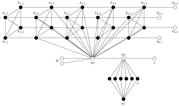
Figure 3. Example of the graph $\mathcal{G}$ with parameters $p=5,o=4,s=6,r=1,q=2$ with strategy vector $X(4)$. Cooperators are depicted by full circles. Note, that this graph exhibits periodic behavior as described in Section 3.2 for $(a,b,c,d)=(1,0.45,1.24,0)$.

The following conditions must be satisfied in order for $\mathcal{X}$ to fulfill (11) and (12).

• The vertices $g_{R},g_{C},g_{D}$ and all vertices in $H,I,J$ keep their strategy. The defector $g_{D}$ must prevent the vertex $g_{R}$ from changing its strategy, must not change its own strategy and must not change the strategy of the cooperators in $J$. This is guaranteed by satisfying the inequalities

  (13) $$\frac{(o+1)a+b}{o+2}<\frac{sc+(r+1)d}{s+r+1}<a\,,$$

  where $a$ is the utility of the vertex $g_{C}$ and the fraction on the left hand side of (13) is an upper bound for the utilities of the cooperating neighbors of $g_{D}$ and $g_{R}$.

• For the cooperation to spread at time $t$, $t=0,\ldots,p-2$, the boundary cooperators in ${K}_{t+1}$ must have greater utility than the boundary defectors in ${K}_{t+2}$, that is,

  (14) $$\min\left\{\frac{(o-1)a+b}{o},\frac{oa+2b}{o+2}\right\}>\frac{c+(o+1)d}{o+2}\,.$$

  Here the first term on the left is the utility of the cooperators in ${K}_{1}$ at $t=0$ and the second term is the utility of boundary cooperators in subsequent time steps.

• The vertex $g_{R}$ must not be stronger than the cooperators in ${K}_{m}$ for $t=0,\ldots,p-2$ and $1\leq m\leq t+1$ for the cooperation to be able to spread, hence

  (15) $$\frac{oa+2b}{o+2}>\frac{(p-2)oc+(o+q+1)d}{(p-1)o+q+1}\,.$$

  Simultaneously, the defecting vertex $g_{R}$ must be able to change the strategy of all neighboring cooperators to defection at time $p-1$, thus

  (16) $$a<\frac{(p-1)oc+(q+1)d}{(p-1)o+q+1}\,.$$

3.2.3. Choosing parameters

We now show that there exists a choice of parameters $o,q,r,s\in\mathbb{N}$ such that the inequalities (13) – (16) are satisfied.

Without loss of generality, we assume $a=1,d=0$ (see [6], Remark 8.). Since the denominators in (15), (16) are positive, we can multiply both sides by the product of the denominators and express $q$ in the terms of $o$. The inequality (15) gives

(17) $$q>\frac{o^{2}\left((1-p)(1-c)-c\right)-o\left(2(p-1)b-2(p-2)c+1\right)-2b}{o+2b}$$

and the inequality (16) gives

(18) $$q<o(p-1)(c-1)-1\,.$$

If we depict both inequalities in the first quadrant of the $o$-$q$ plane, the inequality (17) is satisfied above the line given by the function on the right hand side. The function on the right hand side asymptotically approaches the line with slope

$$\sigma_{1}=(1-p)(1-c)-c\,.$$

The inequality (18) is satisfied below the line with positive slope

$$\sigma_{2}=(p-1)(c-1)>0\,.$$

The difference of the slopes $\sigma_{2}-\sigma_{1}=c>0$ is always positive and we are therefore able to find $o,q\in\mathbb{N}$ such that the inequalities (15) and (16) are satisfied, see Figure 4. Furthermore, we can choose $o,q$ arbitrarily big.

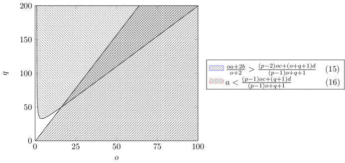
Figure 4. Regions of parameters $o,q$ satisfying the inequalities (15)and (16). The regions are depicted for $(a,b,c,d)=(1,-0.45,1.35,0)$ and $p=10$.

Since $a>d$ holds, the number $o$ can be chosen great enough such that (14) is satisfied.

Since $c>a>d$ holds, we can find integers $r,s\in\mathbb{N}$ (possibly very big ones) such that (13) is satisfied (implicitly using the density of rational numbers and the fact that our parameters are generic).

Thus, we are able to find parameters $o,q,r,s\in\mathbb{N}$ such that the equations (13) – (16) are satisfied and subsequently, $\mathcal{X}$ is a periodic trajectory of $\mathcal{E}=(\mathcal{G},\pi,u,\mathcal{T},\varphi)$ with initial state $X_{0}$ having minimal period length $p$. ∎

4. Periodic orbits on an acyclic graph

Interestingly, periodic behavior of an evolutionary game on a graph can be observed even in the case when the underlying graph is a tree. The absence of cycles demands a new view on the periodic dynamics since the information (strategy change) can spread only gradually through the graph; for example there is no way of ”resetting” vertex strategies. Nevertheless, for specific parameter regions arbitrary long periodic behavior can occur.

Theorem 4.1.

Let $\pi=(a,b,c,d)\in\mathcal{P}$ be admissible parameters satisfying the conditions of the HD scenario, $c>a>b>d$, $u$ the mean utility function, $\mathcal{T}$ the synchronous update order, $\varphi$ deterministic imitation dynamics and $p_{0}\in\mathbb{N}$. There exists an acyclic graph $\mathcal{G}$, a number $p\in\mathbb{N}_{0}$ such that $p\geq p_{0}$ and an initial state $X_{0}$ such that $\mathcal{X}=(X(0),X(1),\ldots)$ is a periodic trajectory of minimal length $p$ of the evolutionary game $\mathcal{E}=(\mathcal{G},\pi,u,\mathcal{T},\varphi)$ on a graph with initial state $X_{0}$.

4.1. Proof of Theorem 4.1

.

4.1.1. The graph and initial state

Let us define a graph $\mathcal{G}$ whose structure is dependent on two parameters $q,r$. The graph $\mathcal{G}$ is a rooted $r$-nary tree such that

• the root $h_{0}$ has only one child $h_{1}$,

• every vertex in level $1$ to $q-2$ has exactly $r$ children,

• exactly $r^{2}$ vertices in level $q-1$ with pairwise different predecessors at level $3$ are leaves,

• every other vertex in level $q-1$ has $r$ children which are leaves.

See Figure 5 for an illustration.

For the sake of simplicity, we focus only on one branch of the tree $\mathcal{G}$ rooted in a fixed vertex $h_{3}$ at level $3$. The vertices in the other branches follow the same dynamics by symmetry reasons (the initial state and the graph $\mathcal{G}$ are invariant with respect to an automorphism exchanging the whole branches rooted at level $3$). The descendant of $h_{1}$ at level $q-1$ in the fixed branch which is a leaf is denoted by $h_{q-1}$. The vertices in a path from $h_{1}$ to $h_{q-1}$ will be denoted by $h_{1},h_{2},\ldots,h_{q-1}$ in an increasing manner. The vertices in $\{h_{1},\ldots,h_{q-1}\}=H$ are called special vertices. The set of all descendants of $h_{m}$ for $m=3,\ldots,q-2$ which are not in $H$ will be denoted by $I_{m}$. Vertices in $I:=\bigcup_{m=3}^{q-2}I_{m}$ are called ordinary vertices.

Let the initial condition $X_{0}$ be such that every vertex in levels $0,\ldots,q-2$ is cooperating and every other vertex is defecting, that is,

$$(X_{0})_{v} =1\,, v\in N_{\leq q-2}(h_{0})\,,$$

$$(X_{0})_{v} =0\,, \text{otherwise}\,.$$

See Figure 5 for illustration of the graph construction and initial condition.

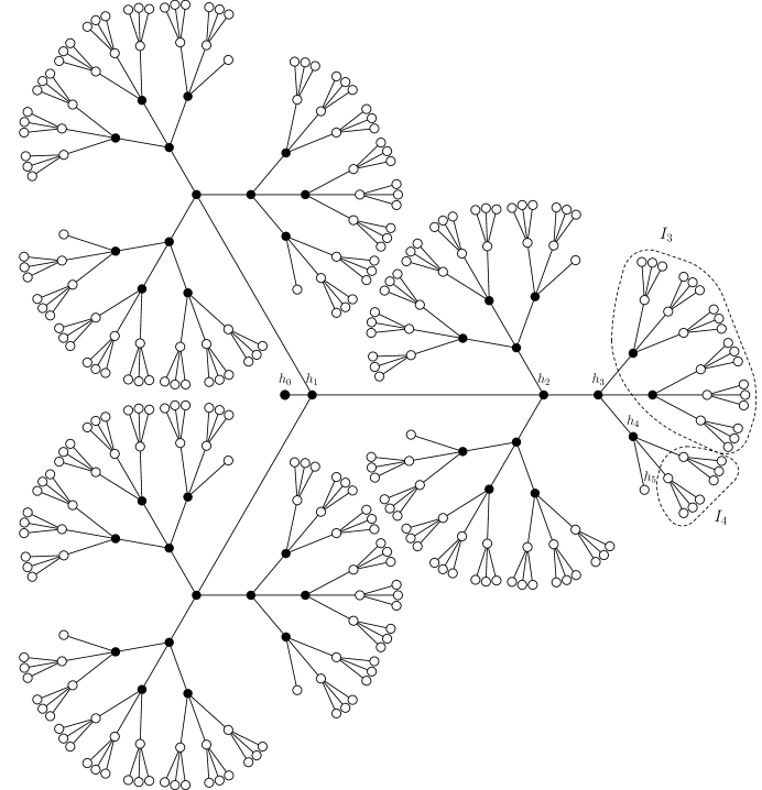
Figure 5. Example of the graph constructed in the proof of Theorem 4.1 with an initial condition. The cooperators are depicted by filled black circles, defectors by white ones. The parameters are $r=3,q=6$

4.1.2. The dynamics

The dynamics of the system in one period can be divided into three qualitatively different phases. There are three important events that occur during one period. At time $t=0$, all vertices at level at most $q-2$ cooperate and all vertices at the levels $q-1$ and $q$ defect. From here, defection is spreading along the special vertices to the root and outward towards the boundary along the ordinary vertices. We call this phase the shrinking phase. At time step $t=q-3$, the only special vertices which cooperate are those at level $0$ and $1$. There are however a few clusters of cooperating ordinary vertices left in the higher levels. Starting from the root, the central cooperating cluster is growing again and at time $t=(q-3)+(q-5)$ there is only this central cluster of cooperators left which encompasses all vertices at level at most $q-4$. Two time steps later, at $t=2(q-3)$, this cluster encompasses all vertices at level at most $q-2$ and we are back at the initial state. Please refer to the example in Section 4.2 and Figures 10–15 for an illustration of the dynamics.

The local dynamics is essentially governed by the following two lemmas.

Lemma 4.2.

Consider parameters $(a,b,c,d)\in\mathcal{P}$ such that

(19) $$\frac{a+rb}{r+1}>\frac{c+rd}{r+1}\,.$$

Let $i$ be a vertex which is a boundary cooperator at time $t$. If $i$ is connected to one cooperator and $r$ boundary defectors, whose defecting neighbors have utility lower that $\frac{a+rb}{r+1}$ and whose only cooperating neighbor is $i$, then $i$ and all of its defecting neighbors will cooperate in the next time step.

Figure 6. Illustration of the local situation in Lemma 4.2. Generally, nothing can be stated about the behavior of the cooperating neighbor on the left.

Proof.

The defecting neighbors of $i$ have utility $\frac{c+rd}{r+1}$, and their defecting neighbors have utility smaller than $\frac{a+rb}{r+1}$. Both of these quantities are lower then the utility of $i$, which is $\frac{a+rb}{r+1}$. ∎

See Figure 6 for an illustration of Lemma 4.2.

Lemma 4.3.

Consider parameters $(a,b,c,d)\in\mathcal{P}$ such that

(20) $$a<\frac{rc+d}{r+1}\,.$$

Let $i$ be a vertex which is a boundary defector at time $t$. If $i$ is connected to one defector and $r$ boundary cooperators, then $i$ and all its neighbors will defect in the next time step.

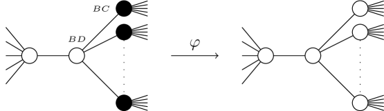
Figure 7. Illustration of the local situation in Lemma 4.3.

Proof.

At time $t$, the vertex $i$ has utility $\frac{rc+d}{r+1}$ which is larger then $a$, the largest utility that a cooperator can achieve. ∎

See Figure 7 for an illustration of Lemma 4.3.

Let $\mathcal{X}=(X(0),X(1),\dots)$ be the trajectory of the evolutionary game on a graph described above with initial state $X_{0}$. We start with some simple observations.

Lemma 4.4.

Let $i$ be an ordinary vertex and let $t\in\mathbb{N}$. All children of $i$ have the same state at time $t$.

Proof.

This follows directly by a symmetry argument. For every pair of children $j_{1}$ and $j_{2}$ of $i$ there is an automorphism of the graph $\mathcal{G}$ that exchanges $j_{1}$ and $j_{2}$. The initial state and the functions defining the dynamics are invariant under such automorphisms of the graph, hence the same must hold for every state in the trajectory. ∎

Lemma 4.5.

Let $i$ be an ordinary vertex. If $X_{i}(t)=0$, then $X_{j}(t+1)=0$ for all children $j$ of $i$.

Proof.

Based on Lemma 4.4 we have to differentiate between only three cases. In the first case all children of $i$ are cooperators. By Lemma 4.3 they will switch to defection. In the second case they are boundary defectors. Therefore all of their children must be cooperators and again Lemma 4.3 shows that they will switch to defection. In the last case the children are inner defectors which can not change their strategy. ∎

The dynamics along the special vertices is very simple to describe. Let $f:\{0,\ldots,2q-6\}\to\mathbb{N}$ be the function given by $f(t):=|t-q+3|+1$, see Figure 8.

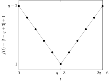
Figure 8. The function $f$ governing the shrinking and expansion of cooperation among the special vertices for $q=8$.

A special vertex $h_{\ell}$ is cooperating at time $t$ if and only if $\ell\leq f(t)$. This is shown together with a description of the dynamics of the strategies of the ordinary vertices in the following theorem. Notice that property (f) and property (g) in Theorem 4.6 immediately imply that $\mathcal{X}$ has period $2q-6$ and property (a) implies that $\mathcal{X}$ has no shorter period.

Theorem 4.6.

The following invariants hold for the dynamics when $0\leq t\leq 2q-6$

1. $$X_{h_{\ell}}(t)=\begin{cases}1&\text{if }\ell\leq f(t)\\ 0&\text{otherwise}\end{cases}, \text{for all }h_{\ell}\in H_{\ell}.$$

2. $h_{\ell}$ is an inner cooperator if and only if $\ell<f(t)$.

3. $h_{\ell}$ is an inner defector if and only if $\ell>f(t)+1$.

In the shrinking phase $(0\leq t<q-3)$ additionally the following properties hold.

1. For $m\leq f(t)+1$ and $i\in I_{m}\cap N_{1}(h_{m})$ we have $X_{i}(t)=1$.

2. For $m>f(t)+1$ and $i\in I_{m}\cap N_{\leq m-f(t)-1}(h_{m})$ we have $X_{i}(t)=0$.

In the expanding phase $(q-3\leq t\leq 2q-6)$, we have

1. All vertices at level at most $f(t)$ are cooperating.

2. All vertices at level $n$ with $f(t)<n\leq f(t)+3$ are defecting.

Proof.

We show by induction that these invariants are true throughout the course of the dynamics. Let $s\in\mathbb{N}$ and assume that the theorem holds for all $t\leq s$.

Initial state; i.e. $s=0$:

Obviously, all of the points (a) - (e) hold true. Since all of the vertices $h_{\ell}$ for $\ell\leq q-3$ are inner cooperators by (b), they preserve their strategy at time $1$. The defecting vertex $h_{q-1}$ has utility $c$. Thus, the vertex $h_{q-2}$ changes its strategy to defection at time $s+1$ while changing the strategy of vertices in $I_{q-2}\cap N_{1}(h_{q-2})$ to cooperation as a consequence of Lemma 4.2. Every other vertex preserve its strategy at time $s=0$ and thus, the points (a) - (e) hold true at time $1$.

Shrinking phase; i.e. $0<s<q-3$:

The vertex $h_{f(s)+1}$ is defecting and has one defecting neighbor $h_{f(s)+2}$ by (a). The children of $h_{f(s)+1}$ are cooperating by (d). Thus, using Lemma 4.3, the vertex $h_{f(s)+1}$ and all of his neighbors are defecting in the next time step. Together with (c), this proves the point (a) for time $s+1$. Using (d), this also immediately implies (b) (the boundary cooperators closest to the root $h_{0}$ of the cluster containing $h_{0}$ are at level $q-2-s$).

The vertices $h_{\ell}$ for $\ell\geq f(s)+1$ are inner defectors by (c). Moreover, their children are all defecting by (e). Thus, $h_{\ell}$ stay inner defectors for $\ell\geq f(s)+1$. The vertex $h_{f(s)}$ is a boundary defector by (b) and has $r$ cooperating neighbors ((d) and (a)). Lemma 4.3 implies the vertex $h_{f(s)}$ is an inner defector at time $s+1$ which is (c) for the next time step.

The invariant (a) implies that the predecessors of all vertices in $I_{m}\cap N_{1}(h_{m})$ are cooperating for $m\leq f(s)+1$. The children of a specific vertex $v$ in $I_{m}\cap N_{1}(h_{m})$ are either all defecting (Lemma 4.4) and then Lemma 4.2 ensures the preservation of cooperation in $s+1$. If the children of $v$ are cooperating then the vertex $v$ is an inner cooperator and preserves its strategy.

As a trivial consequence of Lemma 4.5, if all vertices in $I_{m}\cap N_{\leq m-f(s)-1}(h_{m})$ are defecting for $m>f(s)+1$ then all vertices in $I_{m}\cap N_{\leq m-f(s)}(h_{m})$ are defecting in the next time step. Furthermore, by (c) and (d) we can apply Lemma 4.2 to the vertex $h_{q+s-2}$. This gives (e).

Phase switch; i.e. $s=q-2$:

We already established (a) - (e) at time $s+1$. We still have to show, that (f) and (g) hold at time $s+1$. We have $f(q-3)=1$. There are no ordinary vertices at level one, hence (d) holds at time $s+1$ by (a). This also shows (g) for special vertices. There is also no ordinary vertex at level two and three, hence we only have to show (g) for ordinary vertices at level four. They are contained in $N_{\leq m-2}\cap I_{m}$ for some $m=3$, hence they are defecting at time $s+1$ by (e).

Growing phase; i.e. $q-3\leq s<2q-6$:

Lemma 4.2 together with (f) and (g) implies that all vertices at level at most $f(s)+1$ will cooperate at time $s+1$, hence (f) holds. This also implies (b).

The special vertices $h_{f(s)+2},\dots,h_{q-1}$ are inner defectors by (c) and hence also defect at time $s+1$. Therefore (a) is satisfied. If $f(s)+3<q$, property (g) automatically holds at time $s+1$. Consider $s$ with $f(s)+3<q$. An ordinary vertex at level $f(s)+4$ is either an inner defector at time $s$ and hence defects at time $s+1$ or it has only cooperating children and hence defects by Lemma 4.3. All in all this shows that (g) is also fulfilled. Let $v$ be a child of a special vertex $h_{\ell}$ with $\ell>s+1$. By (c) it is defecting at time $s$. Either it is an inner defector and hence also defects at time $s+1$ or all its children are cooperators and it defects at time $s+1$ by Lemma 4.3. This established in particular that $h_{\ell}$ is an inner defector at time $s+1$, in other words, (g). ∎

4.1.3. Parameter choice

The only assumptions we needed in the dynamics section were the inequalities (19), (20) and the assumption that the parameters $(a,b,c,d)$ satisfy the conditions of the HD scenario $(c>a>b>d)$. Let such $a,b,c,d$ be given. Clearly, $r$ can be chosen great enough such that the inequalities (19) and (20) hold.

The minimal period of the constructed trajectory is $2(q-3)$. Setting $q:=\max\{5,\left\lceil p_{0}/2\right\rceil+3\}$ the period is at least $p_{0}$. ∎

Remark 1.

In the constructions in Sections 3.1 and 3.2, the behaviour of the number of cooperators or more precisely the sequence $(|\{v\in V\;|\;X_{v}(t)=1\}|)_{t\in\mathbb{N}_{0}}$ was rather boring. During one period of the trajectory it was growing and reset to the initial value at the end of the period. The behaviour of this sequence is much more interesting for our tree construction as shown in Figure 9.

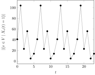
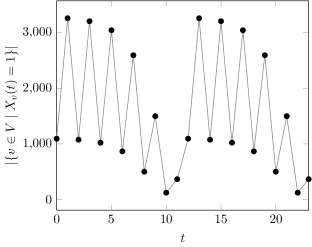
Figure 9. Development of the number of cooperators for the evolutionary game on the tree $\mathcal{G}$ in Section 4 with $r=3$ and game theoretic parameters $(a,b,c,d)=(1,0.7,2,0)$. On the left the tree has depth $q=6$, on the right $q=9$.

4.2. Example

Figures 10 – 15 depict an example of a trajectory on an evolutionary game on a graph constructed in Section 4.1. Cooperators are depicted with black circles, defectors are depicted with white ones. The players changing strategy in the current time step are highlighted with a dashed circle. The parameters of this graph are $r=3,q=6$. This trajectory can be observed for example for parameter vector $(a,b,c,d)=(1,0.6,2,0)$ satisfying the inequalities (19), (20). Note that the inequality

(21) $$b>\frac{c+rd}{r+1}$$

holds for such a choice of parameters. Cooperation then spreads from outer cooperators towards the leaves between $X(2)$ and $X(3)$. In contrary, for $b\in(0,0.5)$ the inequality (21) does not hold anymore. The outer cooperators (cooperators not in the cluster containing the root $h_{0}$) then vanish in $X(3)$ and they do not spread cooperation further. The strategy vectors $X(t)$ and $X(t+6)$ coincide for $t\in\mathbb{N}_{0}$.

This example and an example of an evolutionary game on a graph with $q=7$ and all other parameters remaining the same can be found online in [15].

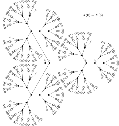
Figure 10. The example from Section 4.2.

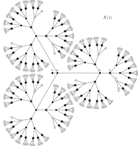
Figure 11. The example from Section 4.2.

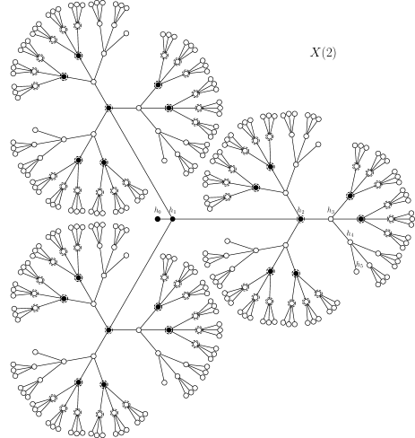
Figure 12. The example from Section 4.2.

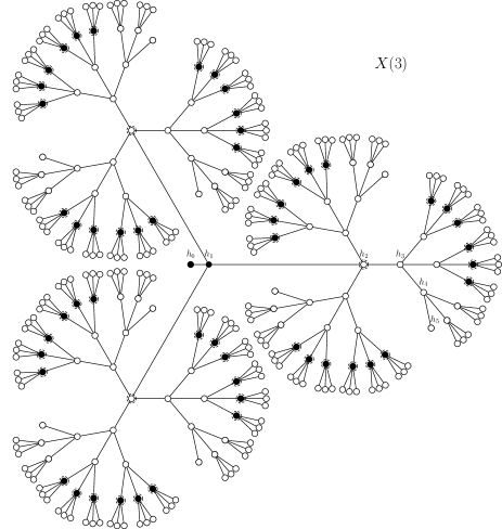
Figure 13. The example from Section 4.2.

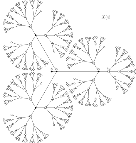
Figure 14. The example from Section 4.2.

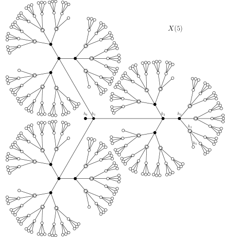
Figure 15. The example from Section 4.2.

5. Conclusion

We showed that on arbitrary graphs the game theoretic parameters can not exclude periodic behavior with long periods. Our proofs hold also true for a small perturbation of the game-theoretical parameters $a,b,c,d$ as a consequence of the generic payoff assumption.

Our constructions rely heavily on the fact that we can choose the graph parameters arbitrarily. This no longer works if we restrict to certain classes of graphs. For example Theorem 4.1 partially answers Question 1 while restricting to the parameters $(a,b,c,d)$ satisfying the conditions of the HD scenario, $c>a>b>d$, and the class of acyclic graphs.

Natural classes of graphs we might restrict ourselves to are $k$-regular graphs (every vertex has exactly $k$ neighbors), vertex-transitive graphs (every pair of vertices can be exchanged by a graph automorphism) or planar graphs (the graph can be drawn in the plane without edge crossings). This leads for example to the following question.

Question 2.

For which game theoretic parameters $(a,b,c,d)$ and positive integers $k,p$ is there a $k$-regular graph $\mathcal{G}$ such that the corresponding evolutionary game with synchronous update and imitation dynamics on $\mathcal{G}$ has a periodic trajectory with minimal period $p$?

References

- [1] G. Abramson and M. Kuperman, Social games in a social network, Physical Review E, 63 (2001), 030901.
- [2] B. Allen and M. A. Nowak, Games on graphs, 1 (2014), 113–151.
- [3] M. Broom and J. Rychtář, Game-Theoretical Models in Biology, 1st edition, CRC Press, Taylor & Francis Group, 2013.
- [4] J. T. Cox, R. Durrett and E. A. Perkins, Voter model perturbations and reaction diffusion equations, vol. 349 of Astérisque, Société Mathématique de France, 2013.
- [5] O. Durán and R. Mulet, Evolutionary prisoner’s dilemma in random graphs, Physica D: Nonlinear Phenomena, 208 (2005), 257–265.
- [6] J. Epperlein, S. Siegmund and P. Stehlík, Evolutionary games on graphs and discrete dynamical systems, Journal of Difference Equations and Applications, 21 (2015), 72–95.
- [7] J. Epperlein, S. Siegmund, P. Stehlík and V. Švígler, Coexistence equilibria of evolutionary games on graphs under deterministic imitation dynamics, Discrete and Continuous Dynamical Systems - Series B, 21 (2016), 803–813.
- [8] J. Hofbauer and K. Sigmund, Evolutionary Games and Population Dynamics, Cambridge University Press, 1998.
- [9] B. J. Kim, A. Trusina, P. Holme, P. Minnhagen, J. S. Chung and M. Y. Choi, Dynamic instabilities induced by asymmetric influence: Prisoners’ dilemma game in small-world networks, Physical Review E, 66 (2002), 021907.
- [10] C. Marr and M.-T. Hütt, Outer-totalistic cellular automata on graphs, Physics Letters A, 373 (2009), 546–549.
- [11] N. Masuda and K. Aihara, Spatial prisoner’s dilemma optimally played in small-world networks, Physics Letters A, 313 (2003), 55–61.
- [12] M. A. Nowak, Evolutionary Dynamics: Exploring the Equations of Life, Belknap Press of Harvard University Press, 2006.
- [13] M. A. Nowak and R. M. May, Evolutionary games and spatial chaos, Nature, 359 (1992), 826–829.
- [14] M. Tomochi, Defectors’ niches: Prisoner’s dilemma game on disordered networks, Social Networks, 26 (2004), 309–321.
- [15] J. Epperlein and V. Švígler, Periodic orbits of an evolutionary game on a tree, https://figshare.com/articles/6-periodic_orbit_of_an_evolutionary_game_on_a_tree/5110981, June 2017, DOI: 10.6084/m9.figshare.5110981.