Effect of Dark Energy Perturbation on Cosmic Voids Formation

Abstract

In this paper, we present the effects of dark energy perturbation on the formation and abundance of cosmic voids. We consider dark energy to be a fluid with a negative pressure characterised by a constant equation of state $w$ and speed of sound $c_{s}^{2}$. By solving fluid equations for two components, namely, dark matter and dark energy fluids, we quantify the effects of dark energy perturbation on the sizes of top-hat voids. We also explore the effects on the size distribution of voids based on the excursion set theory. We confirm that dark energy perturbation negligibly affects the size evolution of voids; $c_{s}^{2}=0$ varies the size only by 0.1% as compared to the homogeneous dark energy model. We also confirm that dark energy perturbation suppresses the void size when $w<-1$ and enhances the void size when $w>-1$ (Basse et al., 2011). In contrast to the negligible impact on the size, we find that the size distribution function on scales larger than 10 ${\rm Mpc}/h$ highly depends on dark energy perturbation; compared to the homogeneous dark energy model, the number of large voids of radius $30{\rm Mpc}$ is 25% larger for the model with $w=-0.9$ and $c_{s}^{2}=0$ while they are 20% less abundant for the model with $w=-1.3$ and $c_{s}^{2}=0$.

Key words: cosmology: large-scale structure of Universe, dark energy.

1 introduction

One of the greatest mysteries in cosmology is the nature of the energy that accelerates the Universe, that is, dark energy (Riess et al., 1998; Perlmutter et al., 1999). The most popular cosmological model, namely, the $\Lambda$CDM model, regards the energy source to be a cosmological constant corresponding to spatially and temporarily uniform energy density. Although the $\Lambda$CDM model best explains various observations (Planck Collaboration et al., 2015; Anderson et al., 2012; Heymans et al., 2013; Suzuki et al., 2012), the theoretical origin of this energy is poorly understood (Weinberg, 1989).

Various models regarding dark energy state that the constant energy density over space and time can be relaxed (Tsujikawa, 2011). If the equation of state of dark energy is not $-1$, the energy density of the dark energy varies with time. If the speed of sound is equal to that of light, the dark energy fluid is regarded as spatially homogeneous because the Jeans length corresponds to the horizon scale. Such dynamical but spatially homogeneous dark energy is usually called quintessence (Zlatev et al., 1999). If the speed of sound of dark energy is smaller than that of light, the dark energy is spatially perturbed, which is realized in models known as k-essence (Chiba et al., 1998; Armendariz-Picon et al., 2000).

One of the most promising tools to reveal the nature of dark energy is large-scale structures (e.g. de Lapparent et al., 1986; Colless, 1998; York et al., 2000). Traditionally, much attention has been paid to high density structures such as clusters of galaxies. Some works have focussed on the impact of dynamical dark energy on structure formation (Wang & Steinhardt, 1998; Chiba et al., 1998; Abramo et al., 2007; Creminelli et al., 2010; Basse et al., 2011; Heneka et al., 2017).

In contrast, low density structures called voids (Gregory & Thompson, 1978) are also considered to probe large-scale structures. Voids occupy a large fraction of volume of the universe (Cautun et al., 2014), and also characterise the matter distribution at a few tens Mpc scales (van de Weygaert, 2016). Recently, various properties of voids have been systematically studied (Pan et al., 2012; Sutter et al., 2012b; Cautun et al., 2014). Voids provide us with independent tools for probing the cosmological models in different manners from overdense objects. Although the voids are described in the quasi linear regime and thus are expected to be more robust probes for large scale structures (van de Weygaert, 2016), defining the voids from data remains ambiguous. Therefore, testing the cosmological model by combining different observables where systematics and cosmological sensitivity are different is essentially important.

Voids are used for constraining cosmological models mainly in two ways so far. Firstly, the shape of the void which is sensitive the dark energy models can be potentially used to constrain cosmology (Park & Lee, 2007; Lee & Park, 2009; Biswas et al., 2010; Bos et al., 2012). The shape of the void is also useful in the context of the Alcock Paczynski (AP) test (Alcock & Paczynski, 1979). The AP test was first applied to the separation of quasar pairs (Phillipps, 1994), and Hu & Haiman (2003) proposed the use of the Baryon Acrostic Oscillation (BAO) ring as a more promising probe. Voids can be also used as the probes for the AP test because the cosmological principle ensures that the voids are expected to be spherical on average (Ryden, 1995; Ryden & Melott, 1996; Lavaux & Wandelt, 2012).

On the contraly, it is known that the shape of void is correlated with each other up to scales more than 30 Mpc (Platen et al., 2008), and thus one needs to take into account such an alignment of voids to avoid a systematic effect when applying voids to the AP test.

Sutter et al. (2012a) first applied the AP test to stacked voids but found no significant signals because the number of voids was insufficient. Sutter et al. (2014) revisited the analysis using the Sloan Digital Sky Survey (SDSS) Data Release 10 (Ahn et al., 2014) and found a substantial signal for the AP test. Recently, Mao et al. (2017) have put a constraint on $\Omega_{m}$ using the AP test on the SDSS Data Release 12 (Alam et al., 2015).

Secondly, voids are used for constraining cosmological models based on their abundance. This statistics is also known to be sensitive to dark energy models (Pisani et al., 2015). The theoretical prediction for void abundance is given by Sheth & van de Weygaert (2004) (the SVdW model). They adopted the excursion set theory (Bond et al., 1991) to predict the mass fraction involved in the void region. They assumed that the abundance of spherically symmetric isolated voids arises when the density contrast becomes less than $\delta_{m}\simeq-0.8$ (Blumenthal et al., 1992). The original SVdW model is inconsistent with both the abundance obtained from N-body simulations and real galaxy distributions. Previous works have extended the SVdW model by relaxing the constant density threshold for void formation, which is calibrated via N-body simulations (Achitouv et al., 2015), or by considering the formation threshold as a free parameter (Chan et al., 2014; Nadathur & Hotchkiss, 2015) in order to obtain a good agreement of the model with the N-body simulations. However, the best-fit values of the formation threshold are not physically interpreted.

With regard to the cosmological constrains using voids, the parameters of the equation of state of dark energy have been well studied in the literature (Pisani et al., 2015) but the inhomogeneity of the dark energy model where dark energy is spatially perturbed has not been focused on very much. Novosyadlyj et al. (2016) studied the effect of dark energy perturbation on the density and velocity profiles of voids. They adopted the universal density profile (Hamaus et al., 2014a) and found that dark energy perturbation negligibly affects the profiles.

In this paper, we investigate the impacts of dark energy perturbation on the evolution of isolated top-hat spherically symmetric voids, focusing on their size and formation epoch. We also study the mechanism by which dark energy perturbation influence void abundance by adopting the SVdW model. We find that the void abundance is remarkably sensitive to dark energy perturbation.

This paper is organised as follows. In Section 2, following the discussion of Basse et al. (2011), we revisit the spherical collapse model under dark energy perturbation and apply it to the spherical void formation. Section 3 is devoted to the numerical results of the void size evolution. In Section 4, we present the dependence of void abundance on dark energy perturbation. We provide a summary in Section 5.

Throughout this work, we assume the cosmological parameters as $h=0.7,\Omega_{m,0}=0.3,$ and $\Omega_{Q,0}=0.7$, which are dimensionless Hubble parameter, density parameters of matter and dark energy, respectively, where we denote the matter component as $m$ the dark energy component as $Q$. In addition, we assume that parameters of the equation of state and the speed of sound are constant, and we take the natural unit of $c=1$.

2 Spherical void formation in the inhomogeneous dark energy model

Void is a structure that on average has an under density profile compared to the mean density of the universe. The density in the centric regions are in general less dense compared to the outer regions. Such a density gradient makes the inner shell of voids expand faster than outer shells. Then matter in a void region accumulates around the void to form dense ridges as their boundaries and such a process results in forming a density profile like a top-hat shape even if we assume a smoothed initial density profiles (Sheth & van de Weygaert, 2004).

On the other hand, Hamaus et al. (2014b) has reported that the spherically averaged density profile of voids in N-body simulations is less steep than expected from the top-hat shape. The difference comes from the fact that individual voids in the realistic situations are not spherical because individual voids are not isolated and their dynamical evolution is highly affected by their local environment. Although an analytic calculation was shown that an isolated void tends to be spherical as it evolves (e.g. Icke, 1984), individual voids do not maintain the shapes at the initial condition and their shapes are far from the spherical ones (Platen et al., 2008). However, if one defines the radial profile by measuring the density on the equidistance contour from the boundary of the void, the stacked profile resembles compensated top-hat shape (Cautun et al., 2016). Therefore, the top-hat profile seems to be a generic property of voids even in the realistic situations (Dubinski et al., 1993; van de Weygaert & van Kampen, 1993; Sheth & van de Weygaert, 2004; van de Weygaert, 2016)

The moment when the inner shells catch up with the outer shells is defined as shell crossing and previous studies have pointed out that the evolution of voids is in full non-linear regime at the moment of shell crossing (Suto et al., 1984; Fillmore & Goldreich, 1984; Bertschinger, 1984). The shell crossing for an isolated spherically symmetric void with a top-hat density profile in the Einstein-de Sitter universe occurs when the density contrast reaches $\delta^{\rm TH}_{m}\simeq-0.8$ (Blumenthal et al., 1992; Dubinski et al., 1993).

Even though a simple model which assumes isolated spherical void with a top-hat profile does not perfectly describe the actual dynamical evolution of voids in the complex environment, starting with such a simplified model can provide us with a lot of insights on the effects of dark energy model. Considering more realistic situations is beyond the scope of this paper and we will explore more detailed study with numerical experiments as a future work. In this section, we describe the formation of a spherically symmetric isolated void with a top-hat density profile in the presence of dark energy perturbation.

In Section 2.1, we revisit the spherically symmetric formation model following the discussion of Basse et al. (2011). In Section 2.2, we extend the model in the presence of dark energy perturbation for constant speed of sound and constant equation of state parameters.

2.1 Spherical symmetric model

To trace the non-linear evolution of voids, we consider a spherically symmetric underdense region with a top-hat profile of radius $R_{\rm v}$. The evolution of the void in an expanding universe follows the equation of motion

$$\frac{1}{R_{\rm v}}\frac{d^{2}R_{\rm v}}{dt^{2}}=-\frac{4\pi G}{3}\sum_{n}(\rho_{n}+3P_{n}),$$ (1)

where $\rho_{n}$ and $P_{n}$ are, respectively, the energy density and pressure of the fluid component $n$ enclosed in the region $r\leq R_{\rm v}$. The density $\rho_{n}$ and pressure $P_{n}$ can be decomposed into unperturbed and perturbed components as

$$\rho_{n}=\bar{\rho}_{n}+\bar{\rho}_{n}\delta_{n},$$ (2)

$$P_{n}=\bar{P}_{n}+\delta P_{n}.$$ (3)

where $\bar{\rho}_{n}$ and $\bar{P}_{n}$ are the mean background values. Since we assume the top-hat density profile, the density contrast can be expressed as

$$\delta_{n}(t,r)=\begin{cases}\ \delta^{\rm TH}_{n}(t)&(0\leq r\leq R_{\rm v}),\\ \ 0&(R_{\rm v}<r).\end{cases}$$ (4)

Given that the void evolves in an expanding universe, equation (1) can be rewritten in terms of the comoving coordinate as

$$\frac{\ddot{X}_{\rm v}}{X_{\rm v}}+{\cal H}\frac{\dot{X}_{\rm v}}{X_{\rm v}}=-\frac{4\pi G}{3}a^{2}\sum_{n}(\bar{\rho}_{n}\delta^{\rm TH}_{n}+3\delta P^{\rm TH}_{n}),$$ (5)

where $X_{\rm v}$, $a$ and ${\cal H}$ represent the comoving radius of the void, scale factor, and conformal Hubble parameter, respectively. The dot denotes the derivative with respect to the conformal time, $d\tau=dt/a$.

2.2 Dark energy perturbation

Now we assume that the universe consists of only dark matter and dark energy. Here we consider the model wherein dark energy and matter are spatially perturbed. Therefore, equation (5) can be written as

$$\frac{\ddot{X}_{\rm v}}{X_{\rm v}}+{\cal H}\frac{\dot{X}_{\rm v}}{X_{\rm v}}=-\frac{4\pi G}{3}a^{2}[\bar{\rho}_{m}\delta^{\rm TH}_{m}+\bar{\rho}_{Q}\delta^{\rm TH}_{Q}+3\delta P^{\rm TH}_{Q}].$$ (6)

In order to solve equation (6), we must simultaneously solve the evolution of matter and dark energy perturbations. Given that the mass of the matter inside a void is conserved,

$$M=\frac{4\pi}{3}\bar{\rho}_{m}(1+\delta_{m}^{\rm TH})R_{\rm v}^{3}=\frac{4\pi}{3}\bar{\rho}_{m}(1+\delta_{m}^{\rm TH})a^{3}X_{\rm v}^{3}.$$ (7)

The matter density perturbation at a given time $\tau$ is simply scaled by the void radius as

$$\delta_{m}^{\rm TH}(\tau)=(1+\delta^{\rm TH}_{m,i})\left[\frac{X_{{\rm v},i}}{X_{\rm v}(\tau)}\right]^{3}-1,$$ (8)

where the variable with subscript $i$ takes the value at the initial time $\tau_{i}$.

In order to introduce the effect of dark energy pressure into a Newtonian regime, we adopt a pseudo Newtonian approach (Lima et al., 1997; Basse et al., 2011). The continuity and Euler equations are given as

$$\dot{\rho}_{Q}+3{\cal H}(\rho_{Q}+P_{Q})+\nabla\cdot[(\rho_{Q}+P_{Q})\bm{v}_{Q}]=0,$$ (9)

$$\dot{{\bm{v}}}_{Q}+{\cal H}{\bm{v}}_{Q}+({\bm{v}}_{Q}\cdot\nabla){\bm{v}}_{Q}+\frac{\nabla P_{Q}+{\bm{v}}_{Q}\dot{P}_{Q}}{\rho_{Q}+P_{Q}}+\nabla\phi=0,$$ (10)

where $\bm{v}_{Q}$ is the velocity of dark energy fluid, and $\phi$ is a gravitational potential that satisfies the Poisson equation,

$$\nabla^{2}\phi=4\pi Ga^{2}[\bar{\rho}_{m}\delta_{m}+\bar{\rho}_{Q}\delta_{Q}+3\delta P_{Q}].$$ (11)

Substituting equations (2) and (3) into (9) and (10) yields the evolution equations for dark energy perturbation;

$$\dot{\delta}_{Q}+3{\cal H}(\delta_{Q}^{P}-w\delta_{Q})+\nabla\cdot[(\rho_{Q}+P_{Q}){\bm{v}}_{Q}/\bar{\rho}_{Q}]=0,$$ (12)

$$\dot{{\bm{v}}}_{Q}+{\cal H}{\bm{v}}_{Q}+({\bm{v}}_{Q}\cdot\nabla){\bm{v}}_{Q}+\frac{\nabla\delta_{Q}^{P}+{\bm{v}}_{Q}(w\dot{\bar{\rho}}_{Q}/\bar{\rho}_{Q}+\dot{\delta}_{Q}^{P})}{1+w+\delta_{Q}+\delta_{Q}^{P}}+\nabla\phi=0,$$ (13)

where $w=\bar{P}_{Q}/\bar{\rho}_{Q}$ is the equation of state of the dark energy component, and $\delta_{Q}^{P}=\delta P_{Q}/\bar{\rho}_{Q}$. We assume that dark energy perturbation is always subdominant compared to matter perturbation. Thus equations (12) and (13) are simplified in the linear perturbation regime as,

$$\dot{\delta}_{Q}^{\rm lin}+3{\cal H}(\delta_{Q}^{\rm P,lin}-w\delta_{Q}^{\rm lin})+(1+w)\theta_{Q}^{\rm lin}=0,$$ (14)

$$\dot{\theta}_{Q}^{\rm lin}+(1-3w){\cal H}\theta_{Q}^{\rm lin}+\frac{\nabla^{2}\delta_{Q}^{\rm P,lin}}{1+w}+\nabla^{2}\phi=0,$$ (15)

where we define the divergence of velocity, $\theta_{Q}=\nabla\cdot{\bm{v}}_{Q}$. As we will see in Section 3, the linear regime assumptions for dark energy perturbation are well satisfied. The above equations can be more easily handled in Fourier space. Since we do not assume the adiabatic condition for dark energy, its pressure perturbation is expressed by density and entropy perturbations. In Fourier space and in the conformal Newtonian gauge, the pressure perturbation for dark energy can be given as (Bean & Doré, 2004)

$$\tilde{\delta}_{Q}^{\rm P,lin}=c_{s}^{2}\tilde{\delta}^{\rm lin}_{Q}+3{\cal H}(1+w)(c_{s}^{2}-w)\tilde{\theta}_{Q}^{\rm lin}/k^{2},$$ (16)

where the speed of sound of dark energy $c_{s}^{2}$ is defined in the dark energy rest frame as

$$c_{s}^{2}=\left.\frac{\delta P_{Q}}{\bar{\rho}_{Q}\delta_{Q}}\right|_{\rm rest}.$$ (17)

The speed of sound of dark energy characterises the typical scale of dark energy perturbation and is assumed to be constant in this work. Owing to the second term in equation (16), the pressure perturbation of dark energy does not vanish even when $c_{s}^{2}=0$.

In Fig. 1, we see that for $c_{s}^{2}=10^{-4}$ the amplitude of the second term is smaller than that of the first term by the factor of at least $10^{-3}$ over all scales inside the horizon, whereas for $c_{s}^{2}=10^{-20}$ the second term dominates over the first term. We note that even for scales well inside the horizon scale, pressure perturbation of dark energy due to entropy perturbation is not negligible for $c_{s}^{2}\ll 1$.

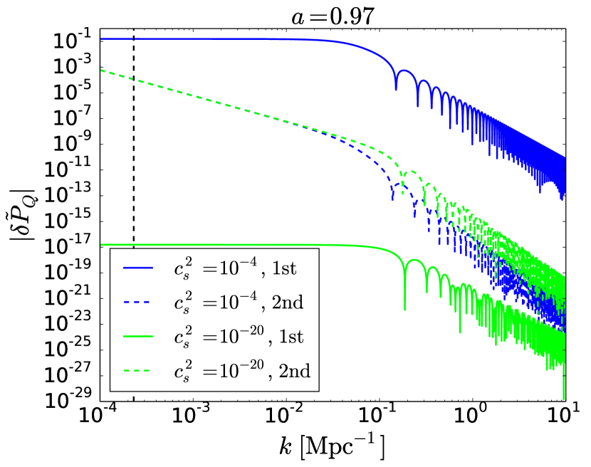
Figure 1: Contributions of the first and second terms to $\tilde{\delta}_{Q}^{\rm P,lin}$ in equation (16) at $a=0.97$. The solid and dashed lines denote the individual contributions of the first and second terms, and the green and blue lines correspond to $c_{s}^{2}=10^{-4}$ and $c_{s}^{2}=10^{-20}$, respectively. For $c_{s}^{2}=10^{-4}$, the second term is smaller than the first term by the factor of $10^{-3}$ even at the horizon scale of the universe which is indicated by the black vertical dashed line. For $c_{s}^{2}=10^{-20}$, the second term dominates the first term over all scales. We use the initial conditions presented in Section 2.3, but set $w=-0.9$ and $M=10^{15}M_{\sun}$. The result is insensitive to the choice of $w$ but the oscillatory damping scale depends on the void mass.

By substituting equation (16) into equation (15) in Fourier space, we obtain

$$\dot{\tilde{\delta}}_{Q}^{\rm lin}+3(c_{s}^{2}-w){\cal H}\tilde{\delta}_{Q}^{\rm lin}+(1+w)\tilde{\theta}^{\rm lin}=0,$$ (18)

$$\dot{\tilde{\theta}}_{Q}^{\rm lin}+(1-3c_{s}^{2}){\cal H}\tilde{\theta}^{\rm lin}-\frac{k^{2}c_{s}^{2}}{1+w}\tilde{\delta}_{Q}^{\rm lin}-k^{2}\tilde{\phi}=0.$$ (19)

We use the Poisson equation in Fourier space along with the above equations,

$$-k^{2}\tilde{\phi}=4\pi Ga^{2}[\bar{\rho}_{m}\tilde{\delta}_{m}+\bar{\rho}_{Q}\tilde{\delta}_{Q}+3\tilde{\delta P}_{Q}].$$ (20)

As can be clearly seen, the dark energy perturbation affects structure formation only thorough the gravitational force through the Poisson equation.

For later convenience, we explicitly give the linearized equations for matter perturbation as follows;

$$\dot{\tilde{\delta}}_{m}^{{\rm lin}}+\tilde{\theta}_{m}^{{\rm lin}}=0,$$ (21)

$$\dot{\tilde{\theta}}_{m}^{{\rm lin}}+{\cal H}\tilde{\theta}_{m}^{{\rm lin}}+4\pi Ga^{2}[\bar{\rho}_{m}\tilde{\delta}_{m}^{{\rm lin}}+\bar{\rho}_{Q}\tilde{\delta}^{\rm lin}_{Q}+3\tilde{\delta P}^{\rm lin}_{Q}]=0.$$ (22)

From equations (18), (19), and (20), eliminating $\theta$ yields the evolution equation of the linear dark energy perturbation;

$$\frac{d^{2}\tilde{\delta}^{\rm lin}_{Q}}{ds^{2}}+{\cal D}(s)\frac{d\tilde{\delta}^{\rm lin}_{Q}}{ds}+\left[\frac{k^{2}c_{s}^{2}}{{\cal H}^{2}}\chi(s)-\kappa(s)\right]\tilde{\delta}^{\rm lin}_{Q}$$

$$\hskip 85.35826pt=\frac{3}{2}(1+w)\Omega_{m}(s)\tilde{\delta}_{m},$$ (23)

where

$$s=\ln a,$$ (24)

$${\cal D}(s)\equiv 1+\frac{1}{\cal H}\frac{d{\cal H}}{ds}-3w,$$ (25)

$$\kappa(s)\equiv 3w\left(1+\frac{1}{\cal H}\frac{d{\cal H}}{ds}\right)+\frac{3}{2}(1+w)\Omega_{Q}(s),$$ (26)

$$\chi(s)\equiv 1+3\frac{{\cal H}^{2}}{k^{2}}\left[1+\frac{1}{\cal H}\frac{d{\cal H}}{ds}-3(c_{s}^{2}-w)\right.$$

$$\hskip 113.81102pt\left.-\frac{3}{2}(1+w)\Omega_{Q}(s)\right].$$ (27)

The evolution equation is numerically solved once the initial condition of the dark energy and matter perturbations are specified as described in the next section.

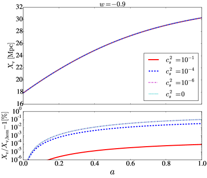
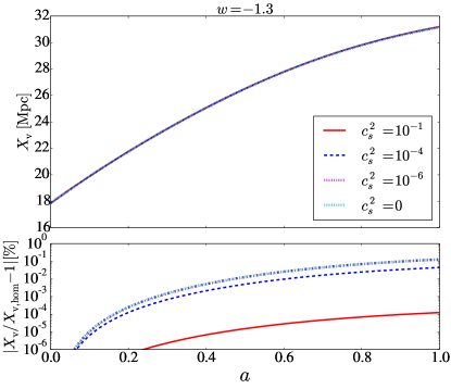
Figure 2: Size evolutions of voids with different speed of sound. We set $w=-0.9$ for the left panels and $w=-1.3$ for the right panels. The speed of sound are $c_{s}^{2}=0,\ 10^{-6},\ 10^{-4}$, and $10^{-1}$ both for the left and right panels. We compare the size evolutions for each value of the speed of sound with the homogeneous dark energy model in the lower panels. The absolute value of fractional difference for the lower right panel corresponds to that the dark energy clustering for $w<-1$ suppresses the void evolution and the difference takes negative values.

2.3 Initial conditions

Now we set up the initial conditions for the calculations.

• Initial time
  Following Basse et al. (2011), we begin our calculation at the cosmic time

  $$t_{i}H_{0}=2.0\times 10^{-6},$$ (28)

  which corresponds to the scale factor,

  $$a_{i}=a_{0}\left(\frac{3t_{i}H_{0}\sqrt{\Omega_{m,0}}}{2}\right)^{2/3}\approx 1.4\times 10^{-4}.$$ (29)

• Initial matter density contrast
  In the EdS universe, linear matter fluctuation evolves in proportion to the scale factor. Thus, at arbitrary time, it scales as

  $$\delta_{m}^{\rm lin}(a)=\frac{a(\tau)}{a_{v}}\delta_{v},$$ (30)

  where $\delta_{v}$ is the critical density for void formation and $a_{v}$ is the scale factor when the linear density contrast reaches $\delta_{v}$. For the EdS universe, we analytically obtain $\delta_{v}=-2.717$ (Blumenthal et al., 1992). If $\delta_{m}^{\rm lin}$ reaches $-2.717$ at the present time, the corresponding initial matter density contrast is $\delta_{m,i}^{\rm lin}\simeq\delta^{\rm TH}_{m,i}=-3.8\times 10^{-4}$ in the EdS universe. For the universe with dark energy, matter growth is suppressed at a later epoch compared to that in the EdS universe. To allow voids to form by the present time, we give a slightly larger negative value of matter density contrast than that in the EdS universe,

  $$\delta_{m,i}^{\rm lin}=\delta^{\rm TH}_{m,i}=-5.0\times 10^{-4},$$ (31)

  where we assume that in the very early epoch the density fluctuation can be well described by the linear perturbation. Note that the choice of the values of initial matter density contrast does not affect the comparison of void size among different dark energy models.

• Initial dark energy density contrast
  We assume that the density contrast of dark energy is proportional to that of matter. Thus once the initial condition of matter is specified, the initial condition of the dark energy perturbation is immediately obtained by numerically integrating equation (23).

• Initial velocity
  We obtain the initial velocity of a void shell by differentiating equation (7),

  $$\left.\frac{dX}{d\tau}\right|_{\tau=\tau_{i}}=\frac{2a_{i}}{3\eta_{i}}\left(1-\frac{1}{3}\delta^{\rm TH}_{m}(\tau_{i})\right)-{\cal H}_{i},$$ (32)

  where $\eta_{i}=\int^{\tau_{i}}_{0}ad\tau$.

2.4 Summary for calculus

To clarify our procedures, here we provide a summary of our calculation steps.

1. We set the initial matter fluctuation and the mass of matter inside to derive the radius of the top-hat initial void by using equation (7).

2. We conduct Fourier transform of $\delta_{m}$ to find $\tilde{\delta}_{m}$ as

   $$\tilde{\delta}_{m}(k,\tau) =\int^{X_{\rm v}}_{0}d^{3}x\ \delta_{m}^{\rm TH}(\tau)\ e^{-i\bm{k}\cdot\bm{x}}$$

   $$=\frac{4\pi}{3}\delta_{m}^{\rm TH}(\tau)X_{\rm v}^{3}(\tau)\tilde{W}(kX_{\rm v}),$$ (33)

   where $\tilde{W}(kX_{\rm v})$ is a top-hat window function in Fourier space,

   $$\tilde{W}(kX_{\rm v})=\frac{3\left[\sin(kX_{\rm v})-kX_{\rm v}\cdot\cos(kX_{\rm v})\right]}{(kX_{\rm v})^{3}}.$$ (34)

   Then we solve the differential equation (23) for $\tilde{\delta}_{Q}^{\rm lin}$.

3. We conduct Fourier inverse transform of $\tilde{\delta}_{Q}^{\rm lin}$ to obtain $\delta^{\rm TH}_{Q}$ in real space, which is averaged out inside the void radius,

   $$\delta^{\rm TH}_{Q}(\tau)=\frac{3}{4\pi X_{\rm v}^{3}}\int d^{3}xW(|\bm{x}|)\delta^{\rm lin}_{Q}(\bm{x},\tau).$$ (35)

   Thus the relation between $\delta_{Q}^{\rm TH}$ and $\tilde{\delta}_{Q}^{\rm lin}$ is

   $$\delta^{\rm TH}_{Q}(\tau)=\int\frac{dk}{2\pi^{2}}k^{2}\tilde{W}(kX_{\rm v}(\tau))\tilde{\delta}^{\rm lin}_{Q}(k,\tau).$$ (36)

4. We solve the second order differential equation for $X_{\rm v}(\tau)$ using the obtained $\delta^{\rm TH}_{m}$ and $\delta_{Q}^{\rm TH}$.

5. Next, we calculate $\delta^{\rm TH}_{m}$ using equation (8)

6. For the next time step, we repeat steps (ii) to (v) untill the matter density fluctuation reaches $\delta^{\rm TH}_{m}=-0.8$.

3 Results of size evolution

In this section, we present the numerical results for the evolution of a spherically symmetric void with a top-hat density profile. We explore the dark energy parameters: $0\leq c_{s}^{2}\leq 1$, $w=-0.9$ and $-1.3$. We also examine the dependence of the void evolution on the void mass. We set the initial mass of $10^{13}M_{\sun}$, $10^{15}M_{\sun}$, and $10^{17}M_{\sun}$. The void mass only affects the void size through equation (7) and the corresponding initial radii are $0.83,18$, and $83{\rm Mpc}$, respectively, in the comoving scale.

3.1 Dependence on $c_{s}^{2}$

In Fig. 2, we show the dependence of the evolution of voids on the speed of sound. We set $w=-0.9$ for the left panel, $w=-1.3$ for the right panel and $M_{i}=10^{15}M_{\sun}$ for both panels. The upper panels show the evolution of void radii; the lower panels show the fractional differences in void radii with respect to that for the homogeneous dark energy model ($c_{s}^{2}=1$). We see that if the speed of sound is low, the deviation is large. For $w=-0.9$ the small speed of sound enhances the size of the void whereas for $w=-1.3$, the small speed of sound suppresses the evolution of voids. We can not find any differences in void size between $c_{s}^{2}=0$ and $c_{s}^{2}=10^{-6}$ for both $w=-0.9$ and $-1.3$ because the void size is larger than the Jeans length of the fluctuations even for $c_{s}^{2}=10^{-6}$.

For both $w=-0.9$ and $-1.3$, the difference in void size between the $c_{s}^{2}=0$ model and the homogeneous dark energy model is of the order of 0.1%. For $c_{s}^{2}=10^{-1}$, the difference is $10^{-4}$% both for $w=-0.9$ and $-1.3$, which is much smaller than that for $c_{s}^{2}=0$. This is because the Jeans length for $c_{s}^{2}=10^{-1}$ is always larger than the void size during evolution. Therefore the effect of enhancement or suppression due to dark energy clustering is negligible.

3.2 Dependence on $w$

In Fig. 2, we see that dark energy perturbation acts in opposite ways depending on the value of $w$: it suppress the evolution of voids for $w<-1$ while it enhances for $w>-1$.

In order to understand these opposite effects, we consider the equation for the evolution of the dark energy perturbation (equation (23)). If $w>-1$, the density contrast of the dark energy component evolves with the same sign as the matter density contrast whereas if $w<-1$, the sign is opposite to the matter component. Then, in equation (5), if the density contrast of dark energy has the same sign as that of matter, the fluctuation of gravitational potential is enhanced, promoting the growth of the voids. Conversely, if the dark energy density contrast has an opposite sign as that of matter, the gravitational potential fluctuation is reduced, suppressing the evolution of void size.

We also see that for $w=-0.9$, dark energy perturbation affects relatively earlier than for $w=-1.3$. This can be simply explained by the domination epoch of dark energy in the cosmic time. In the universe where $w<-1$, dark energy dominates the expansion at a later epoch and therefore, there is less chance that the matter fluctuations are affected by dark energy.

3.3 Dependence on initial mass

In Fig. 3, we plot the evolution of void size with different void masses. We set $w=-0.9$ and $c_{s}^{2}=10^{-4}$ but take values for the initial masses of $10^{13}$, $10^{15}$ and $10^{17}M_{\sun}$. Here we choose $c_{s}^{2}=10^{-4}$ in order to demonstrate the relation between the void size and the Jeans length. As we see in Fig. 4, the Jeans length for $c_{s}^{2}=10^{-6}$ is always smaller than the void size for $M>10^{15}M_{\sun}$. Therefore we do not find any difference in the evolution of void size.

In Fig. 3, we see that the void with larger initial mass is more affected by the dark energy perturbation. As we see in the next section, if the size of a void exceeds the Jeans length of dark energy, the density contrast of dark energy inside the void evolves regardless of the size of the void. However, if the size is less than the Jeans length, the evolution of the dark energy perturbation inside the void is suppressed.

3.4 Evolution of dark energy perturbation

In Fig. 5, we show the evolution of dark energy perturbation in Fourier space for $c_{s}^{2}=10^{-6}$, $10^{-4}$ and $10^{-1}$ and $w=-0.9$ for the $M=10^{15}M_{\sun}$ void. We sample the fluctuations at $k=0.01,0.1$ and $1$ ${\rm Mpc}^{-1}$, which correspond to larger, comparable and smaller scales, respectively, as compared to the void radius. For $c_{s}^{2}=10^{-1}$, $k>k_{J}$ for all three scales at $a<10^{-3}$. Therefore, the perturbation does not grow with time and gradually decays with oscillations.

For $c_{s}^{2}=10^{-4}$, the fluctuation scale of $k=1.0$ ${\rm Mpc}^{-1}$ mode is always smaller than the Jeans length and thus shows the same trend as that for $c_{s}^{2}=10^{-1}$, whereas the scale $k=0.1$ Mpc^-1 becomes closer to the Jeans length at $a=10^{-2}$, and thus, $\tilde{\delta}_{Q}(k=0.1{\rm Mpc}^{-1})$ evolves with time only at an early epoch. Once the scale crosses the Jeans length, it again shows a slight depression with oscillations.

For $c_{s}^{2}=10^{-6}$, $k<k_{J}$ for all three modes at $a<10^{-3}$, and thus $\tilde{\delta}_{Q}$ evolves with time at an early stage and it also decays with oscillation once the scale is close to the Jeans scale. We also note that the amplitude of $\tilde{\delta}_{Q}$ is similar regardless of the value of the speed of sound when $\tilde{\delta}_{Q}$ is in the evolutional phase (see $k=0.01$ Mpc^-1 at $a\ll 1$), whereas it is strongly dependent on $c_{s}^{2}$ once the scale of fluctuation reaches the Jeans length and $\tilde{\delta}_{Q}$ is constant or in an oscillationally decaying phase.

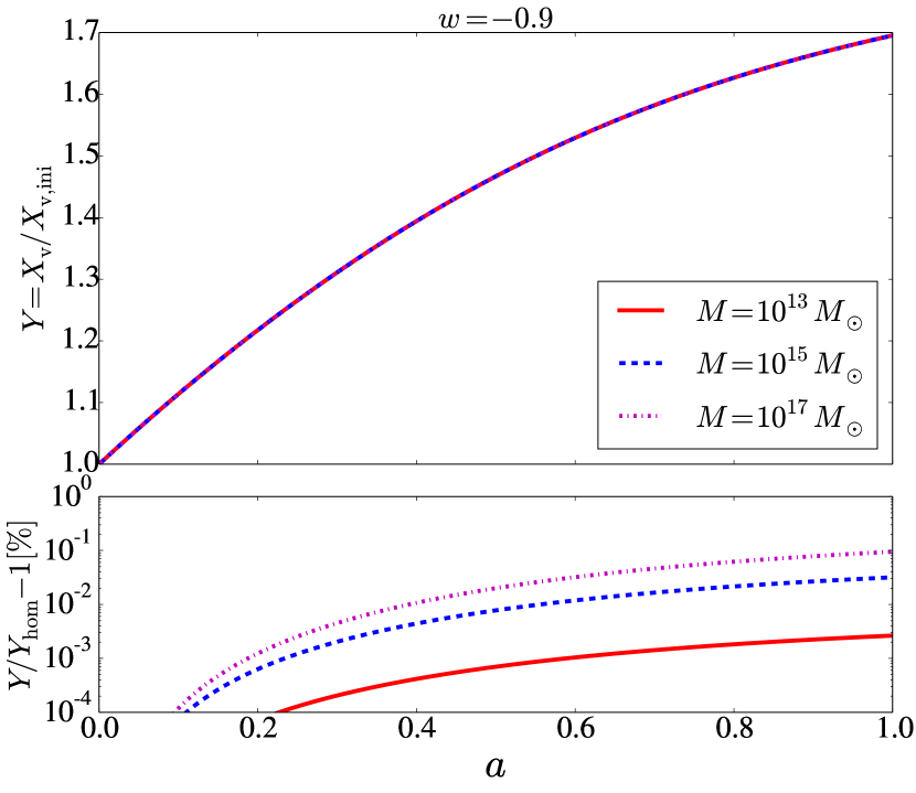
Figure 3: Same as Fig. 2 for $w=-0.9$ and $c_{s}^{2}=10^{-4}$ but for an initial void mass of $10^{13},10^{15}$ and $10^{17}M_{\sun}$. The upper panel displays the void sizes normalised by the initial size. The lower panel shows fractional differences of the void sizes normalised by that in the homogenous dark energy model.

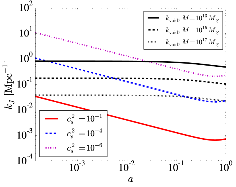
Figure 4: Evolution of the Jeans wavenumbers for each value of speed of sound (coloured lines) and the wavenumber which corresponds to the void radius for each mass scale with $c_{s}^{2}=10^{-1}$(black lines) as indicated in the figure.

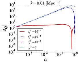
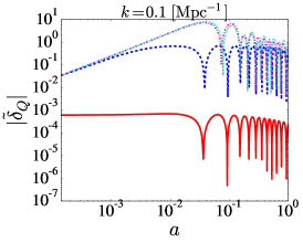
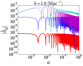
Figure 5: Evolutions of density perturbation of dark energy in Fourier space. The evolution for $k=0.01,0.1$ and $1.0$ Mpc^-1 are shown in the left, middle and right panels, respectively. Each density contrast begins to oscillate when the Jeans length for each value of the speed of sound crosses the wavelength. For calculation, we set $w=-0.9$ and $M=10^{15}M_{\sun}$.

4 Size distribution

Dark energy perturbation also affects the size distribution of voids through the threshold of void formation and the linear matter power spectrum. In this section, we revisit the size distribution of voids derived from the excursion set theory, which was first applied to void formation by Sheth & van de Weygaert (2004), and then we extend the theory to the dark energy perturbation model.

4.1 Excursion set theory for voids

Based on the Press-Schechter formalism (Press & Schechter, 1974), we consider a probability distribution for $\delta_{M}$, which is the smoothed linear density contrast at mass scale $M$ in Lagrangian space. Such a density contrast is expressed as

$$\delta_{M}(\bm{q})=\frac{3}{4\pi R_{L}^{3}}\int_{|\bm{q}^{\prime}-\bm{q}|\leq R_{L}}\delta(\bm{q}^{\prime})d^{3}q^{\prime},$$ (37)

where $\bm{q}$ is a Lagrangian coordinate, and $R_{L}$ is a smoothing scale in Lagrangian space corresponding to the mass scale via $M=4\pi\bar{\rho}_{m}R_{L}^{3}/3=4\pi\bar{\rho}_{m}(1+\delta_{m})R_{\rm v}^{3}/3$ where $R_{\rm v}$ denote the size of voids in the Eulerian space. If the density contrast exceeds a certain threshold $\delta_{c}$, the matter inside $R_{L}$ contributes to the formation of a halo of mass more than $M$. The probability distribution that $\delta_{M}(\bm{q})$ exceeds $\delta_{c}$ with mass between $M$ and $M+dM$ can be interpreted as the fraction of mass between $M$ and $M+dM$ which contributes to the formation of a halo.

In the excursion set theory (EST), we try to find the probability distribution of $\delta_{M}$ given the smoothing scale corresponding to mass $M$, where $\delta_{M}$ first crosses the density threshold (Bond et al., 1991; Zentner, 2007). We assume that the probability distribution of the smoothed density fluctuation follows the Gaussian distribution with mean zero, and variance

$$S=\sigma^{2}(M)=\int\frac{k^{2}dk}{2\pi^{2}}\tilde{W}(kR_{L})P(k).$$ (38)

We define the probability distribution of $\delta_{M}$ on a scale $S$ for the random walk as $\Pi(\delta_{M},S)$. Then, if we begin the trajectory from the horizon scale, we can set the initial condition $\Pi(0,0)=1$. We also assume that the transition probability is Gaussian: thus, the transition from $\Pi(\delta_{M}-\Delta\delta_{M},S)$ to $\Pi(\delta_{M},S+\Delta S)$ is

$$\Pi(\delta_{M},S+\Delta S)=\int d(\Delta\delta_{M})\frac{1}{\sqrt{2\pi\Delta S}}\exp\left(-\frac{(\Delta\delta_{M})^{2}}{2\Delta S}\right)$$

$$\times\Pi(\delta_{M}-\Delta\delta_{M},S).$$ (39)

Expanding the LHS of equation (39) in terms of $S$ and the RHS in terms of $\delta_{M}$, we obtain the diffusion equation,

$$\frac{\partial\Pi}{\partial S}=\frac{1}{2}\frac{\partial^{2}\Pi}{\partial\delta_{M}^{2}}.$$ (40)

As mentioned in Sheth & van de Weygaert (2004), we set two barriers for void formation as a boundary condition for the random walk: linear density thresholds for halo and void formation. For halo formation, $\delta_{c}=1.686$ is often used as the linear density threshold for collapsed objects in the literature, while for void formation, $\delta_{v}=-2.717$ is analytically derived by using spherical model in the EdS universe (Blumenthal et al., 1992; Jennings et al., 2013). This value is defined as the linear density contrast of a void shell crossing when the inner shell catches up with the outer shell: therefore the Lagrangian density at the shell diverges (Sheth & van de Weygaert, 2004). At that moment, the non-linear density contrast inside the void is $\delta^{\rm TH}_{m}\simeq-0.8$.

In order to obtain the void size distribution, we need the probability of the first crossing of the void threshold $\delta_{v}$ on a certain smoothing scale $R_{L}$ without crossing $\delta_{c}$ on any scales larger than $R_{L}$. Any trajectories crossing $\delta_{c}$ before crossing $\delta_{v}$ correspond to the voids which are surrounded by high density regions, and then, eventually disappear during the structure formation (void in cloud). Thus, we exclude those trajectories when we count voids. We consider only the first crossing of $\delta_{v}$ and do not count the voids any longer even if the trajectory crosses $\delta_{v}$ more than once at smaller scales in order to exclude the voids embedded in the larger void (void in void) and to avoid the double counting. The solution of $\Pi(\delta_{M},S)$ with above condition gives the probability distribution of $\delta_{M}$ between $\delta_{v}$ and $\delta_{c}$ on a scale $S$ without crossing $\delta_{c}$ and $\delta_{v}$ on any $S^{\prime}<S$. Thus the fraction of trajectories that $\delta_{M}$ satisfies the condition is

$$F(S)=\int^{\delta_{c}}_{\delta_{v}}\Pi(\delta_{M},S)d\delta_{M}.$$ (41)

Let $f(S)dS$ be the probability that $\delta_{M}$ crosses either of the density thresholds between $S$ and $S+dS$, and such a probability is obtained by subtracting $F(S+dS)$ from $F(S)$. Then,

$$f(S)dS=-\frac{dF(S)}{dS}dS=\left.-\frac{1}{2}\frac{\partial\Pi}{\partial\delta_{M}}\right|^{\delta_{c}}_{\delta_{v}}dS.$$ (42)

The limit of $\delta_{M}=\delta_{c}$ in the RHS of equation (42) is the probability that $\delta_{M}$ crosses $\delta_{c}$ for the first time between $S$ and $S+dS$, whereas the limit of $\delta_{M}=\delta_{v}$ is the probability that $\delta_{M}$ reaches the value $\delta_{v}$. Therefore, the probability that $\delta_{M}$ crosses $\delta_{v}$ for the first time between $S$ and $S+dS$ is

$$f(S)dS =\left.\frac{1}{2}\frac{\partial\Pi}{\partial\delta_{M}}\right|_{\delta_{M}=\delta_{v}}$$

$$=\sum_{n=1}^{\infty}\frac{n\pi D^{2}}{\delta_{v}^{2}}\sin(n\pi D)\exp\left(-\frac{n^{2}\pi^{2}D^{2}}{S}\frac{S}{\delta_{v}^{2}}\right)dS,$$ (43)

where $D=|\delta_{v}|/(\delta_{c}+|\delta_{v}|)$.

The mass function is expressed as

$$\frac{dN}{d\ln M}=\frac{\bar{\rho}}{M}Sf(S)\frac{d\ln S}{d\ln M},$$ (44)

where $N$ is the number density of voids including mass $M$. It is useful to characterise the void by its size instead of mass. Thus, we rewrite the abundance of voids in terms of the size by using the relation,

$$\frac{dN}{d\ln R_{\rm v}}=\frac{dN}{d\ln R_{L}}=3\frac{dN}{d\ln M}.$$ (45)

Finally, we obtain the void size distribution in Eulerian space,

$$\frac{dN}{dR_{\rm v}}=(1+\delta_{m})^{\frac{1}{3}}\left(\frac{3}{4\pi R^{3}_{L}}\right)f(\nu)\frac{d\nu}{dR_{L}},$$ (46)

where $\nu=\delta_{v}^{2}/S$.

We adopt an approximate expression for $f(\nu)$ (Sheth & van de Weygaert, 2004),

$$\nu f(\nu)\approx\sqrt{\frac{\nu}{2\pi}}\exp\left(-\frac{\nu}{2}\right)\exp\left(-\frac{|\delta_{v}|}{\delta_{c}}\frac{D^{2}}{4\nu}-2\frac{D^{4}}{\nu^{2}}\right).$$ (47)

The dark energy perturbation affects the number of void in two ways. First, the dark energy perturbation affects $\nu$ through the variance, equation (38). We calculate the linear power spectrum $P(k)$ using the publicly available code, CAMB (Lewis et al., 2000) to derive $S$ for the dark energy perturbation model. Second, the dark energy perturbation affects the density threshold for cosmic voids. We solve equations (21), (22) and (23) to find the linear density threshold corresponding to the non-linear density fluctuations of $\delta_{m}=-0.8$ (Blumenthal et al., 1992).

4.1.1 Dependence on $c_{s}^{2}$

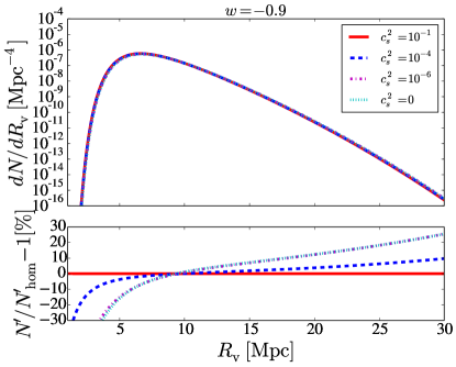
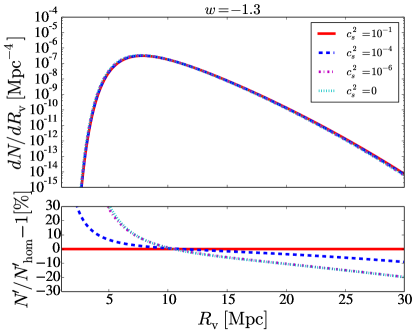
Figure 6: Comparison of the abundance of voids at present time. We fix $w=-0.9$ (left) and $w=-1.3$ (right), and the values of speed of sound as $c_{s}^{2}=0,10^{-6},10^{-4},10^{-1}$. The lower panels show the fractional difference from the homogeneous dark energy model with the same equation of state parameter, where $N^{\prime}=dN/dR_{\rm v}$. For both $w$, the deviation from the case for homogeneous dark energy is noticeable at larger radii: more than $10\%$ for $c_{s}^{2}=0$ for 30 Mpc voids.

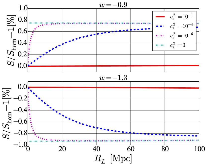
Figure 7: Comparison of variance at present time. We set $w=-0.9$ for the upper panel and $w=-1.3$ for the lower panel. Both panels show the fractional difference from the homogeneous dark energy model.

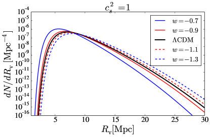
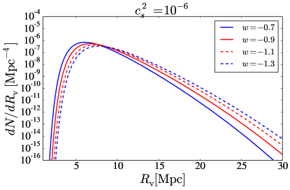
Figure 8: Comparison of the abundance of voids for different equation of state parameters for fixed speed of sound. We set $c_{s}^{2}=1$ (left) and $c_{s}^{2}=10^{-6}$ (right). Models with $w<-1$ enhance the number of voids with large radii whereas they suppresses the number of smaller voids. These effects are more prominent in the absence of dark energy perturbation.

4.2 Results

In this section, we demonstrate the numerical results for the effect of the dark energy perturbation on void abundance.

Figure 6 shows the size distribution of voids at the present time. The size distribution does not show any differences between $c_{s}^{2}=10^{-1}$ and the homogeneous dark energy model ($c_{s}^{2}=1$) for both $w=-0.9$ and $-1.3$. For $w=-0.9$ and $c_{s}^{2}<10^{-4}$, the number of large voids with a radius of $30$ Mpc is larger by more than 10 % compared with the homogeneous dark energy model, whereas small voids with radii smaller than $10$ Mpc decrease.

For $w=-1.3$, the dark energy perturbation works in a manner opposite to that for the $w=-0.9$ model; the dark energy perturbation suppresses the number of large voids and enhances the number of small voids. For $c_{s}^{2}<10^{-4}$, the number of voids of radius of $30$ Mpc is suppressed by also more than $10\%$ as compared with that in the homogeneous dark energy model.

We see almost no difference in void abundance between $c_{s}^{2}=0$ and $10^{-6}$. As described in Section 3, the Jeans length for $c_{s}^{2}=10^{-6}$ is sufficiently smaller than the void radius, and therefore, large voids are affected by the dark energy perturbation in a similar manner in the $c_{s}^{2}=0$ and $10^{-6}$ models.

According to the results of Section 3, for individual voids with radius $R_{\rm v}\sim 30\ {\rm Mpc}$ at present time ($a=1$), the deviation of the radius from the homogeneous dark energy model is of the order of 0.1%. In contrast, the deviation of the abundance from that for the homogeneous dark energy model is of the oder of 10%. The difference in void abundance mainly arises from the difference in variance $S$. As shown in Fig. 7, for $w=-0.9$, the deviation in $S$ with $c_{s}^{2}=0$ from the homogeneous dark energy model at a smoothing scale $R_{L}$ = 30 Mpc is about 0.75 %, while for $w=-1.3$ such deviation is -0.94%. In addition, the size function includes the exponential, and therefore, the deviation in the size function is significant.

We also see drastic deviations at smaller scales which have the opposite trend for larger scales. For larger scales, the first exponential term in equation (47) mainly contributes to the abundance of voids. For $w=-0.9$ we see that the variance with dark energy perturbation is enhanced as compared with the homogeneous dark energy model, indicating that the argument of the exponential approaches $0$ when there is dark energy perturbation which leads to an increase in the abundance of large voids. In contrast for small scales, the second exponential term contributes to the abundance and the argument of the exponential rapidly drops in the presence of dark energy perturbation, suppressing the abundance of small voids.

For $w=-1.3$ the difference in variance between the inhomogeneous and homogeneous dark energy models have opposite signs as compared with the case of $w=-0.9$. Thus, the abundance of voids is enhanced on smaller scales and suppressed on larger scales in the presence of dark energy perturbation.

We also confirm that the peak of the abundance is approximately at $R=5\sim 10$ Mpc. Furthermore, we find that different values of the speed of sound lead to different peak locations in the size function. Compared with the $c_{s}^{2}=0$ case, the position of the peak shifts to larger scale by 1.3% whereas it shifts smaller scale by 1.5% for $w=-1.3$ when $c_{s}^{2}=10^{-1}$.

4.2.1 Dependence on $w$

Figure 8 shows the void abundance for a fixed value of the speed of sound but different equation of state. We see that $w<-1$ models increase the number of voids with radius larger than $10$ Mpc, while $w>-1$ models increase that of voids on scales smaller than $10$ Mpc. These enhancements are smaller for the inhomogeneous dark energy model than for the homogeneous dark energy model. For example, the number of voids with $R_{\rm v}=30$ Mpc for $w=-1.3$ is about 1500 times larger than that for $w=-0.7$ for the homogeneous dark energy model, whereas for the $c_{s}^{2}=10^{-6}$ model it is only about 280 times larger.

As we have seen in previous sections, the sign of dark energy perturbation is different depending on whether $w$ is greater or less than $-1$. Therefore, when $w$ is less negative, the dark energy perturbation causes an increase in the number of large scale voids while it leads to a decrease in that of the small scale voids. In contrast, when $w$ is more negative, dark energy perturbation affects in an opposite manner to the case of $w>-1$ so that the number of large voids is suppressed while that of small voids is enhanced.

5 Summary

We investigated the effects of dark energy perturbation on the formation of cosmic voids. We treated the speed of sound and the equation of state of dark energy as constant parameters in our model. We studied the dependence of the formation of an isolated spherically symmetric void on these parameters and the initial size of the void. We found that the effects of the different values of the speed of sound and initial sizes are much small. These results are broadly consistent with those of Novosyadlyj et al. (2016), and may lead us to the conclusion that the dark energy perturbation does not greatly affect void formation.

We also investigated the effects of the dark energy perturbation on the abundance of voids based on the EST. We found that the differences between the homogeneous and inhomogeneous dark energy models are significant when the speed of sound is much smaller than that of light.

For both $w=-0.9$ and $w=-1.3$, the difference in the size of voids with an initial mass of $10^{15}M_{\sun}$ between the cases of $c_{s}^{2}=1$ and $c_{s}^{2}={0}$ is of the order of 0.1% at present time. In contrast, the difference in the abundance of the corresponding voids is more than 20 %. As the size function has an exponential tail at larger scales, a subtle change in the void size may cause a drastic amplification of the void abundance.

References

- Abramo et al. (2007) Abramo L. R., Batista R. C., Liberato L., Rosenfeld R., 2007, JCAP, 11, 012
- Achitouv et al. (2015) Achitouv I., Neyrinck M., Paranjape A., 2015, MNRAS, 451, 3964
- Ahn et al. (2014) Ahn C. P. et al., 2014, ApJS, 211, 17
- Alam et al. (2015) Alam S. et al., 2015, ApJS, 219, 12
- Alcock & Paczynski (1979) Alcock C., Paczynski B., 1979, Nature, 281, 358
- Anderson et al. (2012) Anderson L. et al., 2012, MNRAS, 427, 3435
- Armendariz-Picon et al. (2000) Armendariz-Picon C., Mukhanov V., Steinhardt P. J., 2000, Physical Review Letters, 85, 4438
- Basse et al. (2011) Basse T., Eggers Bjælde O., Wong Y. Y. Y., 2011, JCAP, 10, 038
- Bean & Doré (2004) Bean R., Doré O., 2004, Phys. Rev. D, 69, 083503
- Bertschinger (1984) Bertschinger E. W., 1984, in Bulletin of the American Astronomical Society, Vol. 16, p. 486
- Biswas et al. (2010) Biswas R., Alizadeh E., Wandelt B. D., 2010, Phys. Rev. D, 82, 023002
- Blumenthal et al. (1992) Blumenthal G. R., da Costa L. N., Goldwirth D. S., Lecar M., Piran T., 1992, ApJ, 388, 234
- Bond et al. (1991) Bond J. R., Cole S., Efstathiou G., Kaiser N., 1991, ApJ, 379, 440
- Bos et al. (2012) Bos E. G. P., van de Weygaert R., Dolag K., Pettorino V., 2012, MNRAS, 426, 440
- Cautun et al. (2016) Cautun M., Cai Y.-C., Frenk C. S., 2016, MNRAS, 457, 2540
- Cautun et al. (2014) Cautun M., van de Weygaert R., Jones B. J. T., Frenk C. S., 2014, MNRAS, 441, 2923
- Chan et al. (2014) Chan K. C., Hamaus N., Desjacques V., 2014, Phys. Rev. D, 90, 103521
- Chiba et al. (1998) Chiba T., Sugiyama N., Nakamura T., 1998, MNRAS, 301, 72
- Colless (1998) Colless M., 1998, Anglo-Australian Observatory Epping Newsletter, 85, 4
- Creminelli et al. (2010) Creminelli P., D’Amico G., Noreña J., Senatore L., Vernizzi F., 2010, JCAP, 3, 027
- de Lapparent et al. (1986) de Lapparent V., Geller M. J., Huchra J. P., 1986, ApJL, 302, L1
- Dubinski et al. (1993) Dubinski J., da Costa L. N., Goldwirth D. S., Lecar M., Piran T., 1993, ApJ, 410, 458
- Fillmore & Goldreich (1984) Fillmore J. A., Goldreich P., 1984, ApJ, 281, 9
- Gregory & Thompson (1978) Gregory S. A., Thompson L. A., 1978, ApJ, 222, 784
- Hamaus et al. (2014a) Hamaus N., Sutter P. M., Wandelt B. D., 2014a, Physical Review Letters, 112, 251302
- Hamaus et al. (2014b) Hamaus N., Wandelt B. D., Sutter P. M., Lavaux G., Warren M. S., 2014b, Physical Review Letters, 112, 041304
- Heneka et al. (2017) Heneka C., Rapetti D., Cataneo M., Mantz A. B., Allen S. W., von der Linden A., 2017, ArXiv e-prints
- Heymans et al. (2013) Heymans C. et al., 2013, MNRAS, 432, 2433
- Hu & Haiman (2003) Hu W., Haiman Z., 2003, Phys. Rev. D, 68, 063004
- Icke (1984) Icke V., 1984, MNRAS, 206, 1P
- Jennings et al. (2013) Jennings E., Li Y., Hu W., 2013, MNRAS, 434, 2167
- Lavaux & Wandelt (2012) Lavaux G., Wandelt B. D., 2012, ApJ, 754, 109
- Lee & Park (2009) Lee J., Park D., 2009, ApJL, 696, L10
- Lewis et al. (2000) Lewis A., Challinor A., Lasenby A., 2000, ApJ, 538, 473
- Lima et al. (1997) Lima J. A. S., Zanchin V., Brandenberger R., 1997, MNRAS, 291, L1
- Mao et al. (2017) Mao Q., Berlind A. A., Scherrer R. J., Neyrinck M. C., Scoccimarro R., Tinker J. L., McBride C. K., Schneider D. P., 2017, ApJ, 835, 160
- Nadathur & Hotchkiss (2015) Nadathur S., Hotchkiss S., 2015, MNRAS, 454, 2228
- Novosyadlyj et al. (2016) Novosyadlyj B., Tsizh M., Kulinich Y., 2016, ArXiv e-prints
- Pan et al. (2012) Pan D. C., Vogeley M. S., Hoyle F., Choi Y.-Y., Park C., 2012, MNRAS, 421, 926
- Park & Lee (2007) Park D., Lee J., 2007, Physical Review Letters, 98, 081301
- Perlmutter et al. (1999) Perlmutter S. et al., 1999, ApJ, 517, 565
- Phillipps (1994) Phillipps S., 1994, MNRAS, 269, 1077
- Pisani et al. (2015) Pisani A., Sutter P. M., Hamaus N., Alizadeh E., Biswas R., Wandelt B. D., Hirata C. M., 2015, Phys. Rev. D, 92, 083531
- Planck Collaboration et al. (2015) Planck Collaboration et al., 2015, ArXiv e-prints
- Platen et al. (2008) Platen E., van de Weygaert R., Jones B. J. T., 2008, MNRAS, 387, 128
- Press & Schechter (1974) Press W. H., Schechter P., 1974, ApJ, 187, 425
- Riess et al. (1998) Riess A. G. et al., 1998, AJ, 116, 1009
- Ryden (1995) Ryden B. S., 1995, ApJ, 452, 25
- Ryden & Melott (1996) Ryden B. S., Melott A. L., 1996, ApJ, 470, 160
- Sheth & van de Weygaert (2004) Sheth R. K., van de Weygaert R., 2004, MNRAS, 350, 517
- Suto et al. (1984) Suto Y., Sato K., Sato H., 1984, Progress of Theoretical Physics, 71, 938
- Sutter et al. (2012a) Sutter P. M., Lavaux G., Wandelt B. D., Weinberg D. H., 2012a, ApJ, 761, 187
- Sutter et al. (2012b) Sutter P. M., Lavaux G., Wandelt B. D., Weinberg D. H., 2012b, ApJ, 761, 44
- Sutter et al. (2014) Sutter P. M., Pisani A., Wandelt B. D., Weinberg D. H., 2014, MNRAS, 443, 2983
- Suzuki et al. (2012) Suzuki N. et al., 2012, ApJ, 746, 85
- Tsujikawa (2011) Tsujikawa S., 2011, in Astrophysics and Space Science Library, Vol. 370, Astrophysics and Space Science Library, Matarrese S., Colpi M., Gorini V., Moschella U., eds., p. 331
- van de Weygaert (2016) van de Weygaert R., 2016, in IAU Symposium, Vol. 308, The Zeldovich Universe: Genesis and Growth of the Cosmic Web, van de Weygaert R., Shandarin S., Saar E., Einasto J., eds., pp. 493–523
- van de Weygaert & van Kampen (1993) van de Weygaert R., van Kampen E., 1993, MNRAS, 263, 481
- Wang & Steinhardt (1998) Wang L., Steinhardt P. J., 1998, ApJ, 508, 483
- Weinberg (1989) Weinberg S., 1989, Reviews of Modern Physics, 61, 1
- York et al. (2000) York D. G. et al., 2000, AJ, 120, 1579
- Zentner (2007) Zentner A. R., 2007, International Journal of Modern Physics D, 16, 763
- Zlatev et al. (1999) Zlatev I., Wang L., Steinhardt P. J., 1999, Physical Review Letters, 82, 896