Spatial dynamics analysis of polarized atom vapor

X.Y.Hu School of Instrumentation Science and Opto-Electronics Engineering, Beihang University, Beijing 100191, China. H.F.Dong School of Instrumentation Science and Opto-Electronics Engineering, Beihang University, Beijing 100191, China. H.C.Huang School of Instrumentation Science and Opto-Electronics Engineering, Beihang University, Beijing 100191, China. L.Chen School of Instrumentation Science and Opto-Electronics Engineering, Beihang University, Beijing 100191, China. Y.Gao School of Instrumentation Science and Opto-Electronics Engineering, Beihang University, Beijing 100191, China.

Abstract

We analyze the spatial dynamics of polarized atom vapor and present a mathematical method to eliminate the diffusion effect partially. It is found that the diffusion effect of polarized atoms can be regarded as a low pass filter in spatial frequency domain and fits well with a Butterworth filter. The fitted spatial filter can be used to restore the original magnetic image before being blurred by the diffusion, thus improving the magnetic spatial resolution. The results of spatial dynamics simulation and magnetic image restoration show the potential usage of this method in magnetic gradiometer and atomic magnetic microscopy.

Bloch equation; spatial dynamics; magnetometer; diffusion; polarized atom

pacs:

78.20.Ls, 87.57.nf

I Introduction

The temporal and spatial dynamics of polarized atom vapor is described by Bloch equationBloch, W. Hansen, and Packard (1946), which is the basic model in fields such as nuclear magnetic resonance(NMR)Hinshaw and Lent (1983); Lehmberg (1972), atomic magnetometerSavukov (2015); Allred et al. (2002); Fang et al. (2014) and atomic gyroscopesDong et al. (2011); Kornack, Ghosh, and Romalis (2005). In these applications the temporal dynamics of polarized atom vapor is analyzed theoretically and verified experimentally. As most of the applications measure the average polarization of atoms in the vapor cell, the spatial dynamics is usually ignored in the modeling and analysis. In the case of gradiometer or array measurements, the diffusion is thought as the essential limit for the spatial resolutionKominis et al. (2003); Giel et al. (2000); Kim et al. (2014).

Inspired by the work of D. Giel et al, who pointed out that the space-time evolution of polarization can be expanded in terms of spatial periodic functionsGiel et al. (2000), we introduce the spatial frequency response of the input magnetic field, which can describe the spatial dynamics of polarized atom vapor in nonuniform magnetic field. MATLAB Simulink is used to simulate the polarized atom vapor system. By setting the magnetic field distribution as one dimensional (1D) sinusoidal waves with different spatial frequency, we get the evolution of the atom polarization in both time and space domain. The result shows that the response decreases when spatial frequency of magnetic field increases, just like a low pass spatial filter, which can be fitted well to a Butterworth filter. Assuming the diffusion effect is isotropy, it can be expanded directly to a two dimensional (2D) spatial filter. By reversing the 2D filter, we obtain a 2D high pass filter that can be used to eliminate diffusion effect and restore the original image partially.

The paper is organized as follows: After a brief introduction of background and motivation in section I, Section II describes the model and parameters calculation used in the simulation. Section III illustrates and discusses the results of spatial dynamics simulation. Finally, conclusions are summarized in section IV.

II MODELING AND PARAMETERS

The Bloch equation can be written with diffusion term as followingLedbetter et al. (2008); Torrey (1956):

\frac{\partial}{\partial t}\overrightarrow{P}=D\nabla^{2}\overrightarrow{P}+\gamma\overrightarrow{B}\times\overrightarrow{P}+R_{p}(s-\overrightarrow{P})-\frac{\overrightarrow{P}}{T_{1},T_{2}}

(1)

where $\overrightarrow{P}$ is the polarization of alkali atoms, D is the diffusion coefficient, $\gamma$ is the gyromagnetic ratio, $\overrightarrow{B}$ is the magnetic field, $R_{p}$ is the pumping rate and $T_{1}$ and $T_{2}$ are the relaxation times for polarization components parallel and transverse to $\overrightarrow{B}$ , respectively. The four terms on the right-hand side describe diffusion, precession, pumping and relaxation, respectively.

To simplify Eq1 and obtain the numerical result of spatial dynamics, we assume the pumping beam and the probing beam are along z axis and x axis, respectively, and the direction of the magnetic field is along y axis. Besides, we also suppose that atoms are fully polarized using a high power short pulse beam. The polarization vector precesses freely in x $-$ z plane after the pumping pulse. In this condition, $P_{y}$ , $T_{1}$ and $R_{p}$ can be ignored and Eq.(1) can be simplified as below:

\frac{\partial}{\partial t}\left[\begin{array}[]{c}P_{x}\\ P_{z}\\ \end{array}\right]=D\nabla^{2}\left[\begin{array}[]{c}P_{x}\\ P_{z}\\ \end{array}\right]+\gamma{B_{y}}\left[\begin{array}[]{c}-P_{z}\\ P_{x}\\ \end{array}\right]-R_{r}\left[\begin{array}[]{c}P_{x}\\ P_{z}\\ \end{array}\right]

(2)

where relaxation rate $R_{r}=1/T_{2}$ and diffusion coefficient D can be calculated according to the experimental setup.

Considering that the atom vapor cell can be antirelaxation coated, or buffered with high pressure gas and can work under spin-exchange relaxation free (SERF) regime, wall collision relaxation and spin-exchange relaxation can be neglected. Moreover, as we measure the local field instead of the average field in the vapor cell, gradient broadening can also be ignored. So the relaxation rate $R_{r}$ is mainly decided by the spin destructionKornack (2006),

R_{r}\approx R_{s}d=\bar{\upsilon}_{\alpha}\sigma^{sd}_{\alpha}n_{\alpha}+\bar{\upsilon}_{q}\sigma^{sd}_{q}n_{q}+\bar{\upsilon}_{b}\sigma^{sd}_{b}n_{b}

(3)

where the first term denotes the collision between alkali atoms themselves, the second term denotes the quench collision and the third term denotes the collision between alkali atom and buffer gas atom. $\bar{\upsilon},\sigma^{sd}$ and n are the relative velocity, collision cross-section of collision pair and density of atoms, respectively. The subscripts $\alpha$ , q and b are for alkali atoms, quenching gas atoms and buffer gas atoms, respectively. The diffusion coefficient depends on the temperature and the pressure of the gasGiel et al. (2000),

D=D_{0}\left(\frac{P_{0}}{P}\right)\left(\frac{T}{T_{0}}\right)^{3/2}

(4)

where $T_{0}=273.15K$ is the standard temperature, $P_{0}=760Torr$ is the standard pressure and $D_{0}$ is the standard diffusion coefficient at $T_{0}$ and $P_{0}$ . Standard diffusion coefficients of Cesium atom in He and $N_{2}$ are $0.39cm^{2}/s$ Ishikawa et al. (1999) and $0.087(15)cm^{2}/s$ Manalis (1972), respectively, which are used in our choice of D in section III.

III NUMERICAL SIMULATION AND RESULTS ANALYSIS

III.1 Spatial frequency response simulation

In the simulation, $R_{r}=300s^{-1}$ and D = 0 $\sim$ 1 $cm^{2}/s$ are choosed according to section II with typical parameters in the atom vapor polarization experiments. And to obtain the spatial frequency response we set $B_{y}$ as a magnetic field with spatial sinusoidal distribution on z axis and $B_{x}=B_{z}=0$ . Thus the input magnetic field can be written as

B_{y}(z)=B_{0}\sin(\omega z)

(5)

where $B_{0}$ is the magnetic amplitude, $\omega$ is the spatial angular frequency and z is the spatial position along z axis.

By simulating the model in Eq.(2) with diffusion term, we can get the temporal and spatial polarization $\hat{P}_{x}(z,t_{d})$ . Then the output magnetic field can be calculated by,

\hat{B}_{y}(z)=\frac{\arcsin(-\hat{P}_{x}(z,t_{d})\emph{e}^{R_{r}t_{d}})}{2\pi\gamma t_{d}}

(6)

pulse pumping magnetometer for different D and $\omega$ . Time delay $t_{d}=10\mu s$ and relaxation rate $R_{r}=300s^{-1}$ .

According to our simulation, $\hat{B}_{y}(z,t_{d})$ also follows the sinusoidal distribution with the same spatial frequency, i.e., $\hat{B}_{y}(z)\approx\hat{B}_{0}\sin(\omega z)$ .We get the corresponding magnetic amplitude $\hat{B}_{0}$ of different $\omega$ , $t_{d}$ and D. With a certain time delay $t_{d}$ the amplitude magnification ${\hat{B}_{0}}/{B_{0}}$ decreases when spatial angular frequency $\omega$ increases, as shown in Fig.1.

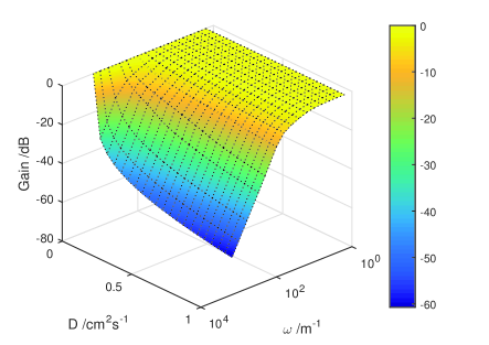
Refer to caption — Figure 1: (Color Online) Amplitude response of the short pulse pumping magnetometer for different D and $\omega$ . Time delay $t_{d}$ =10s and relaxation rate $R_{r}=300s^{-1}$ .

The figure also shows that the cutoff spatial frequency of the system decreases with the increase of diffusion coefficient.

III.2 Reverse approximation of diffusion process

Fig.2

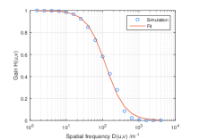
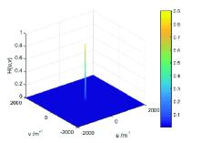
is the spatial response when $t_{d}=\rm 10\mu s$ and $D=\rm 0.6cm^{2}/s$ , which can be fitted well with a Butterworth filter $1/\sqrt{1+(\omega/\omega_{0})^{2n}}$ . The phase response of Butterworth filter is ignored due to the isotropy of diffusion. The corresponding 2D Butterworth filter can be expressed as

H(u,v)=\frac{1}{1+(D(u,v)/D_{0})^{2n}}

(7)

where $D(u,v)$ is the distance between a point $(u,v)$ in the frequency domain and the center of the frequency rectangle, and $D_{0}$ is the cutoff frequencyGonzalez and Woods (2009). Fig. 2 illustrates the corresponding 2D spatial filter, which is expanded from the fitted curve of Fig. 2.

As the 2D filter in Fig. 2 is generated by the spatial frequency response of Bloch equation simulation, it approximately represents the diffusion effect. Furthermore, we can restore the original magnetic image with a reversed 2D filter $1-H(u,v)$ in Fig. 2.

To provide a better view of the restoration effect, we simulate the atom vapor system in magnetic field of two close magnetic dipoles, and assume the dipoles is small enough to ignore the magnetic field inside the dipoles. The magnetic field $B_{y}$ vaires inversely with the third power of distance in $y-z$ plane, as show in Fig.3 .

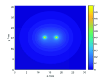
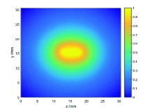
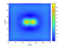
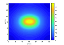
The measured magnetic image simulated using Bloch model, i.e. Eq.(2), and 2D filter, i.e. Eq.(7), are displayed in Fig. 3 and Fig. 3, respectively, where the two dipoles can hardly be distinguished. With a reversed 2D filter $1-H(u,v)$ , we get the restored image from Fig. 4 and the result is shown in Fig. 3. In the restored image, the two dipoles can be distinguished again and thus the spatial resolution is improved. The slightly diffrence between Fig. 3 and Fig. 3 may be due to the fit error in the high frequency part.

IV Conclusion

In summary, the spatial dynamics of polarized atom vapor is analyzed based on the Bloch equation and short pulse pumping and probe scheme. The simulated spatial frequency response fits well with a low pass Butterworth filter. By passing the magnetic image through the reversed spatial fitter, we eliminate partially the diffusion effect and increase the spatial resolution of the image. This analysis and restoration method can be used in spatial magnetometry, such as magnetic gradiometer and atomic magnetic microscopy.

Acknowledgement

The authors thank the support by National Natural Science Foundation of China under Grant No. 61074171 and 61273067 and National Program on Key Basic Research Project of China (2012CB934104). The authors would like to thank Dr. Iannis K. Kominis for the beneficial discussion on spatial resolution, which is another great inspiration to the idea of this paper.

References

Bloch, W. Hansen, and Packard (1946) F. Bloch, W. W. Hansen, and M. Packard, “Nuclear induction,” APS Journals, 69 (1946).
Hinshaw and Lent (1983) W. S. Hinshaw and A. H. Lent, “An introduction to nmr imaging: From the bloch equation to the imaging equation,” Proceedings of the IEEE 71, 338–350 (1983).
Lehmberg (1972) R. H. Lehmberg, “Modification of bloch’s equations at optical frequencies,” Optics Communications 5, 152–156 (1972).
Savukov (2015) I. Savukov, “Gradient-echo 3d imaging of rb polarization in fiber-coupled atomic magnetometer,” Journal of Magnetic Resonance 256, 9–13 (2015).
Allred et al. (2002) J. C. Allred, R. N. Lyman, T. W. Kornack, and M. V. Romalis, “High-sensitivity atomic magnetometer unaffected by spin-exchange relaxation.” Physical Review Letters 89, 130801 (2002).
Fang et al. (2014) J. Fang, T. Wang, H. Zhang, Y. Li, and S. Zou, “Optimizations of spin-exchange relaxation-free magnetometer based on potassium and rubidium hybrid optical pumping,” Review of Scientific Instruments 85, 123104 (2014).
Dong et al. (2011) H. Dong, J. Fang, J. Qin, and Y. Chen, “Analysis of the electrons-nuclei coupled atomic gyroscope,” Optics Communications 284, 2886–2889 (2011).
Kornack, Ghosh, and Romalis (2005) T. W. Kornack, R. K. Ghosh, and M. V. Romalis, “Nuclear spin gyroscope based on an atomic comagnetometer,” Physical Review Letters 95, 230801 (2005).
Kominis et al. (2003) I. K. Kominis, T. W. Kornack, J. C. Allred, and M. V. Romalis, “A subfemtotesla multichannel atomic magnetometer,” Nature 422, 596–599 (2003).
Giel et al. (2000) D. Giel, G. Hinz, D. Nettels, and A. Weis, “Diffusion of cs atoms in ne buffer gas measured by optical magnetic resonance tomography,” Optics Express 6, 251–6 (2000).
Kim et al. (2014) K. Kim, S. Begus, H. Xia, S. K. Lee, V. Jazbinsek, Z. Trontelj, and M. V. Romalis, “Multi-channel atomic magnetometer for magnetoencephalography: A configuration study,” Neuroimage 89, 143–151 (2014).
Ledbetter et al. (2008) M. P. Ledbetter, I. M. Savukov, V. M. Acosta, D. Budker, and M. V. Romalis, “Spin-exchange-relaxation-free magnetometry with cs vapor,” Phys. Rev. A 77, 033408 (2008).
Torrey (1956) H. C. Torrey, “Bloch equations with diffusion terms,” Phys. Rev. 104, 563–565 (1956).
Kornack (2006) T. W. Kornack, “A test of cpt and lorentz symmetry using a potassium-helium-3 co-magnetometer,” (2006).
Ishikawa et al. (1999) K. Ishikawa, Y. Anraku, Y. Takahashi, and T. Yabuzaki, “Optical magnetic-resonance imaging of laser-polarized cs atoms,” J. Opt. Soc. Am. B 16, 31–37 (1999).
Manalis (1972) M. S. Manalis, “Nonthermal saha equation and the physics of a cool dense helium plasma,” Phys. Rev. A 5, 993–994 (1972).
Gonzalez and Woods (2009) R. C. Gonzalez and R. E. Woods, Digital Image Processing (Pearson Education Asia ltd, 2009).