Theorems on Entanglement Typicality in Non-equilibrium Dynamics

Abstract

The notion of typicality in statistical mechanics is essential to characterize a macroscopic system. An overwhelming majority of the pure state looks almost identical if we neglect macroscopic non-local correlations, suggesting that thermal equilibrium is the collection of the typical properties. Quantum entanglement, which characterizes a non-local correlation, also has a typical behavior in equilibrium systems. However, it remains elusive whether there is a typical behavior of entanglement in dynamical non-equilibrium systems. To investigate the typicality, we consider a situation where a system in a pure state starts to share entanglement with its environment system due to the interaction between them. Assuming the initial state is randomly chosen from an ensemble of pure states, a criteria for the typicality of the Rényi entropies is presented. In addition, it is analytically proven that the second Rényi entropy has a typical behavior in two cases. The first one is an energy dissipation process in a multiple-qubit system which is initially in a random pure state in an energy shell. Since the typical behavior is qualitatively the same as the prediction of the Page curve conjecture, it gives the first proof of the Page curve conjecture in a dynamical process. In the second case, the typicality is proven for any dynamics described by a multiple-product of a single-qudit channel when the system is initially in a pure state randomly chosen from the whole Hilbert space. This result shows that entanglement typicality is not a specific feature of energy dissipating processes.

TU-1061

I Introduction

Typicality is one of the essential concepts in macroscopic systems. The Sugita theorem Sugita shows that macroscopic observables composed of the sum of local operators cannot distinguish an overwhelmingly majority of pure states in an energy shell, which implies that if we neglect macroscopic non-local correlations, almost all of the pure states look quite similar to each other. This mathematical fact allows us to make a postulate that thermal equilibrium is the collection of the typical behaviors Tasaki . Then, what we practically observe in an equilibrium system is predictable by using the microcanonical ensemble average. Typicality gives an intuitive explanation for the existence of the arrow of time in macroscopic systems Lebowitz . It should be noted that this interpretation of thermal equilibrium is not directly related to the longstanding argument on the ergodicity in classical systems as a justification of the microcanonical ensemble. Actually, it is known that the “ergodic time” is too long to give a sufficient justification for a possible time-average in a realistic experiment Bricmont . Since the Sugita theorem does not rely on the detailed dynamics of the system, it explains the reason why thermal equilibrium is so ubiquitous, and suggests that thermodynamic properties may be useful to investigate a system whose dynamics remains unknown. In fact, although black holes do not seem to be a normal thermodynamic system, it is known that they have thermodynamics-like laws Bardeen_Carter_Hawking , and that they emit the Hawking radiation whose spectrum is thermal in the semi-classical approximation of the quantum gravity theory Hawking_rad .

There is another well-known typical feature in macroscopic equilibrium systems — typicality of entanglement. Entanglement characterizes a non-local nature of the system, which is quantified by various kinds of measures such as the entanglement entropy and the Rényi entropy. The Lubkin–Lloyd–Pagels–Page (LLPP) theorem Lubkin ; Lloyd_Pagels ; Page_sub shows that a small subsystem typically shares almost maximal entanglement with its complement system, if the total macroscopic system is in a pure state randomly chosen from the whole Hilbert space according to the Haar measure. This distribution of state corresponds to the microcanonical ensemble for a system with a trivial free Hamiltonian $H=0$, or a system at infinite temperature where its free Hamiltonian is effectively negligible. Nevertheless, it is not hard to expect that, in a system with a nontrivial Hamiltonian at a finite temperature, the typical entanglement entropy is approximately given by its maximum, i.e., the thermal entropy of the smaller subsystem. A heuristic explanation is that the ordinary statistical mechanical argument suggests the smaller subsystem is well described by the Gibbs state, which is supported by the Sugita theorem. By using the cTPQ state formulation Sugiura_Shimizu , a universal feature of typical Rényi entropies at a finite temperature has been derived, and it is shown that the universal behavior is reproduced for eigenstates in a non-integrable system but not in an integrable system Fujita_Nakagawa_Sugiura_Watanabe . In Vidmar_Hackl_Bianchi_Rigol , it is shown that the average of entanglement entropy over the eigenstates in a translationally invariant system with quadratic fermionic Hamiltonian is different from the original result of the LLPP theorem. All these results reveal the typical feature of entanglement in an isolated equilibrium system in the sense that the total system is assumed to be in a pure state randomly chosen according to an ensemble.

Entanglement in non-equilibrium macroscopic systems is also of interest. In the context of quantum channel capacity, whose asymptotic theory essentially deals with a macroscopic system, it is known that entanglement can enhance the transmission rate for noisy channels Bennett_Shor_Smolin_Thapliyal . Calculations on the time evolution of the entanglement entropy in globally quenched systems show that there is a maximum speed of propagation of the signal Calabrese_Cardy , as expected from the causality. In Fujita_Nakagawa_Sugiura_Watanabe , it has been checked that the time evolution of the second Rényi entropy in a quenched system is well fitted by the universal behavior derived in the paper for both a non-integrable and an integrable system. In the context of the AdS/CFT correspondence Maldacena , it has been shown that the holographic entanglement entropy for a very small subsystem has the first law-like relationship for static and translationally invariant excited states Bhattacharya_Nozaki_Takayanagi_Ugajin . This result is extended to the entanglement for spherical subsystems in a time-dependent excited state Nozaki_Numasawa_Prudenziati_Takayanagi . In Fan_Zhang_Shen_Zhai , it has been proven that the time evolution of the second Rényi entropy in a quenched system is related with the out-of-order correlation, which is important in the analysis of quantum chaos. Besides these theoretical investigations, the second Rényi entropy has been detected in recent ultracold atom experiments EE_exp1 ; EE_exp2 , suggesting that the time evolution of macroscopic entanglement may also be measured in future experiments.

In modern arguments on resolution scenarios for the black hole information loss paradox, time evolution of entanglement between the black hole and the Hawking radiation plays a significant role. In the semi-classical approximation, it is shown that there remains the Hawking radiation in a mixed state after the complete evaporation of a black hole Hawking_BHIP . Considering a black hole formed by a quantum field in a pure state, it is often argued that this evaporation process indicates the loss of quantum information and/or the violation of unitarity. The mixedness of the Hawking radiation can be understood by the entanglement between the Hawking radiation and the black hole. In the semi-classical approximation, it is known that there is a partner mode inside the black hole which purifies each Hawking mode Hotta_Schutzhold_Unruh , meaning that the entanglement monotonically increases in time. This entanglement makes the Hawking radiation mixed. If the quantum gravity theory is unitary, there must be the purification partner of the Hawking radiation. Possible known candidates for the partner are the Hawking radiation itself Page_curve ; Almheiri_Marolf_Polchinski_Sully ; Almheiri_Marolf_Polchinski_Stanford_Sully , remnants Aharonov_Casher_Nussinov , zero-point fluctuation Wilczek ; Hotta_Schutzhold_Unruh , degrees of freedom in baby universe Unruh_Wald and soft hairs Hawking_Perry_Strominger .

In the pioneering work done by Page Page_curve , it is conjectured that a time evolution of the entanglement entropy between a black hole and the Hawking radiation is given by the typical behavior derived by using the LLPP theorem. Under the assumption that the total system is always in a random pure state, and that the evaporation process is described by the change in the dimensions of the Hilbert spaces for the Hawking radiation and the black hole, the typical entanglement entropy is given by the thermal entropy of the smaller subsystem. This evolution curve of entanglement is called the Page curve. One interesting aspect of its prediction is that it predicts that the entanglement entropy after the half-evaporation time, called the Page time, is given by the Bekenstein–Hawking entropy Bekenstein ; Hawking_rad . It is difficult to check the validity of the conjecture in a realistic black hole evaporation process since the quantum gravity theory has not been established completely. For black holes with negative heat capacity, the composite system of the black hole and the Hawking radiation has an instability Hawking_instability , meaning that the Page curve conjecture seems to be doubtful since the total system cannot be in a thermal equilibrium. In an analysis on a black hole evaporation qubit model with negative heat capacity Hotta_Nambu_Yamaguchi , it is pointed out that the emission of soft hair may make the entanglement larger than the Page curve, which would avoid the emergence of the firewall Almheiri_Marolf_Polchinski_Sully ; Almheiri_Marolf_Polchinski_Stanford_Sully . It should be noted that the Page curve conjecture does not rely on any detailed dynamics of black holes. Thus, an analysis in a condensed matter system has an implication for the validity of the conjecture.

The main objective of this paper is not to discuss the validity of the Page curve in black hole evaporation processes but to investigate a typical entanglement in a dynamical process from a general perspective. In a macroscopic system, it is difficult to calculate the time evolution of the entanglement exactly, even when one knows the initial state. Rather, the success of the equilibrium statistical mechanics suggests that typical features have fundamental importance. We prepare the initial state as a pure state randomly chosen from a subset of the total Hilbert space. The system interacts with the environment system and starts to share entanglement. We derive a general formula for the average and the standard deviation of the trace of the $m$-th power of the state to investigate the typicality of $m$-th Rényi entropy. Once one could show that the ratio of the standard deviation to the average is exponentially small as the system size becomes large, Chebyshev’s inequality ensures the probability of getting an atypical value is also exponentially small, meaning that we practically observe the average value in a macroscopic system. Although it is quite difficult to prove the typicality for general dynamics, we provide two cases where the typicality of the second Rényi entropy can be proven analytically. The first one is an energy dissipation process in a multiple-qubit system, which is similar to the situation in the Page curve conjecture. We show that at the very last stage of the dissipation process, the typical value behaves similar to the Rényi entropy calculated by the Gibbs state. This is the “first proof” of the Page curve conjecture as a dynamical process. In the second case, we investigate the typicality for a multiple-qudit system under the assumption that the system is initially in a pure state distributed over the whole Hilbert space. It is shown that the second Rényi entropy has a typical behavior for any process composed of a tensor product of a single-qudit quantum channel, meaning that the typicality of entanglement is not a specific feature of an energy dissipation process.

This paper is organized as follows. In Section II, we derive a formula for the average and the standard deviation for the trace of $m$-th power of state. In addition, a general magnitude relationship between them is proven. In Section III, we analytically prove the typicality of the second Rényi entropy for two kinds of cases. In Section IV, we summarize our conclusions.

II Ensemble average and Variance

Let us consider a system $A$ in a pure state $\ket{\Psi}_{A}\in\mathcal{H}_{A}$ at the initial time. When the system $A$ interacts with the environment system $E$, these two subsystems start to share entanglement. The most general time evolution of the system $A$ can be described by a quantum channel $\mathcal{E}_{A}$, and it will evolve into $\rho_{A}\equiv\mathcal{E}_{A}\left(\ket{\Psi}_{A}\bra{\Psi}_{A}\right)$. In general, the output state $\rho_{A}$ can be a state for a system different from $A$. Just for simplicity, let us assume the output system is the same as the original one. It is easy to extend the results below for a nontrivial output system. Entanglement between the system $A$ and its environment can be quantified by using the $m$-th Rényi entropy $R_{m}$ defined by

$$R_{m}\equiv\frac{1}{1-m}\ln{\left(\mathrm{Tr}\left(\rho_{A}^{m}\right)\right)}.$$ (1)

Rényi entropy is related with the entanglement entropy $S_{\mathrm{EE}}\equiv-\mathrm{Tr}\left(\rho_{A}\ln{\rho_{A}}\right)=\lim_{m\to 1}R_{m}$.

In order to investigate the typicality of entanglement, let us consider an ensemble of the initial state $\ket{\Psi}_{A}$ which is distributed according to the Haar measure of the unitary group on a sub-Hilbert space $\mathcal{H}_{S}\subset\mathcal{H}_{A}$. The most important example of ensemble is the microcanonical ensemble, where the state is chosen uniformly from an energy shell. Introducing an orthonormal basis of the $\mathcal{H}_{S}$ as $\{\ket{i}_{A}\}_{i=1}^{d_{S}}$, a Haar-random state can be expanded as $\ket{\Psi}_{A}=\sum_{i=1}^{d_{S}}X_{i}\ket{i}_{A}\in\mathcal{H}_{S}$, where $d_{S}\equiv\dim{\mathcal{H}_{S}}$ and $\{X_{i}\}$ are random coefficients. The detailed definition of $\{X_{i}\}$ is given in Appendix A. Then,

$$\rho_{A}(\{X_{i}\})=\sum_{i,j=1}^{d_{S}}X_{i}X_{j}^{*}\mathcal{E}_{A}\left(\ket{i}_{A}\bra{j}_{A}\right)$$ (2)

describes the state evolved by $\mathcal{E}_{A}$. The ensemble average of $R_{m}$ is given by

$$\overline{R_{m}} =\frac{1}{1-m}\overline{\ln{\left(\mathrm{Tr}\left(\rho_{A}\left(\{X_{i}\}\right)^{m}\right)\right)}}$$

$$=\frac{1}{1-m}\overline{\ln{\left(\mathrm{Tr}\left(\prod_{k=1}^{m}\sum_{i^{(k)},j^{(k)}=1}^{d_{S}}X_{i^{(k)}}X_{j^{(k)}}^{*}\mathcal{E}_{A}\left(\ket{i^{(k)}}\bra{j^{(k)}}\right)\right)\right)}},$$ (3)

where the overline denotes the integration over the Haar measure. It is difficult to calculate the average of logarithm of random coefficients ${X_{i}}$ directly. Instead, let us use the following quantity:

$$\tilde{R}_{m}\equiv\frac{1}{1-m}\ln{\left(\overline{\mathrm{Tr}\left(\rho_{A}\left(\{X_{i}\}\right)^{m}\right)}\right)},$$ (4)

which is obtained by calculating the average of the trace of $m$-th power of $\rho\left(\left\{X_{i}\right\}\right)$:

$$\overline{\mathrm{Tr}\left(\rho_{A}\left(\{X_{i}\}\right)^{m}\right)}=\overline{\prod_{k=1}^{m}\sum_{i^{(k)},j^{(k)}=1}^{d_{S}}X_{i^{(k)}}X_{j^{(k)}}^{*}}\mathrm{Tr}\left(\prod_{l=1}^{m}\mathcal{E}_{A}\left(\ket{i^{(l)}}\bra{j^{(l)}}\right)\right).$$ (5)

If the standard deviation divided by the average of $\mathrm{Tr}\left(\rho_{A}\left(\{X_{i}\}\right)^{m}\right)$ is exponentially small in $N$, then the typical value $\overline{R_{m}}$ is approximately given by $\tilde{R}_{m}$. A similar argument can also be found in Fujita_Nakagawa_Sugiura_Watanabe .

As is derived in Appendix A,

$$\overline{\prod_{k=1}^{m}X_{i^{(k)}}X_{j^{(k)}}^{*}}=\frac{\Gamma(d_{S})}{\Gamma(d_{S}+m)}\sum_{\tau\in S_{m}}\prod_{k=1}^{m}\delta_{j^{(k)},i^{(\tau(k))}},$$ (6)

where $S_{m}$ denotes the symmetric group of degree $m$. By using this formula, the average and the variance of $\mathrm{Tr}\left(\rho_{A}\left(\{X_{i}\}\right)^{m}\right)$ for arbitrary positive integer $m$ can be obtained, although they are complicated. The average is given by

$$\overline{\mathrm{Tr}\left(\rho_{A}\left(\{X_{i}\}\right)^{m}\right)}=\frac{\Gamma(d_{S})}{\Gamma(d_{S}+m)}\sum_{\tau\in S_{m}}\sum_{i^{(1)},\cdots,i^{(m)}=1}^{d_{S}}\mathrm{Tr}\left(\prod_{k=1}^{m}\mathcal{E}_{A}\left(\ket{i^{(k)}}\bra{i^{(\tau(k))}}\right)\right).$$ (7)

On the other hand,

$$\overline{\left(\mathrm{Tr}\left(\rho_{A}\left(\{X_{i}\}\right)^{m}\right)\right)^{2}}$$

$$=\frac{\Gamma(d_{S})}{\Gamma(d_{S}+2m)}\sum_{\tau\in S_{2m}}\sum_{i^{(1)},\cdots,i^{(2m)}=1}^{d_{S}}\mathrm{Tr}\left(\prod_{k=1}^{m}\mathcal{E}_{A}\left(\ket{i^{(k)}}\bra{i^{(\tau(k))}}\right)\right)\mathrm{Tr}\left(\prod_{l=m+1}^{2m}\mathcal{E}_{A}\left(\ket{i^{(l)}}\bra{i^{(\tau(l))}}\right)\right).$$ (8)

$S_{2m}$ contains a subset $S_{m}\times S_{m}$ which is composed of a product of elements in $S_{m}$ in the sense that

$$\begin{pmatrix}1&2&\cdots&m&m+1&m+2&\cdots&2m\\ \tau_{1}(1)&\tau_{1}(2)&\cdots&\tau_{1}(m)&m+\tau_{2}(1)&m+\tau_{2}(2)&\cdots&m+\tau_{2}(m)\end{pmatrix}\in S_{2m},$$ (9)

where $\tau_{1},\tau_{2}\in S_{m}$. Thus, the ratio of Eq (8) to the square of Eq (7) is given by a product of

$$\frac{\frac{\Gamma(d_{S})}{\Gamma(d_{S}+2m)}}{\left(\frac{\Gamma(d_{S})}{\Gamma(d_{S}+m-1)}\right)^{2}}=\frac{d_{S}(d_{S}+1)\cdots(d_{S}+m-1)}{(d_{S}+m)(d_{S}+m+1)\cdots(d_{S}+2m-1)}$$ (10)

and

$$1+\frac{\sum_{\tau\in S_{2m}\backslash S_{m}\times S_{m}}\sum_{i^{(1)},\cdots,i^{(2m)}=1}^{d_{S}}\mathrm{Tr}\left(\prod_{k=1}^{m}\mathcal{E}_{A}\left(\ket{i^{(k)}}\bra{i^{(\tau(k))}}\right)\right)\mathrm{Tr}\left(\prod_{l=m+1}^{2m}\mathcal{E}_{A}\left(\ket{i^{(l)}}\bra{i^{(\tau(l))}}\right)\right)}{\left(\sum_{\tau\in S_{m}}\sum_{i^{(1)},\cdots,i^{(m)}=1}^{d_{S}}\mathrm{Tr}\left(\prod_{k=1}^{m}\mathcal{E}_{A}\left(\ket{i^{(k)}}\bra{i^{(\tau(k))}}\right)\right)\right)^{2}}.$$ (11)

If $d_{S}$ grows exponentially fast as the system size becomes large, the first factor is given by $1$ plus an exponentially small term. For example, if we take $\mathcal{H}_{S}$ as an Hilbert space spanned by energy eigenstates in an energy shell, this condition is satisfied for a normal thermodynamic system. Since the variance is given by

$$\overline{\left(\mathrm{Tr}\left(\rho_{A}\left(\{X_{i}\}\right)\right)-\overline{\mathrm{Tr}\left(\rho_{A}\left(\{X_{i}\}\right)\right)}\right)^{2}}=\overline{\left(\mathrm{Tr}\left(\rho_{A}\left(\{X_{i}\}\right)^{2}\right)\right)^{2}}-\left(\overline{\mathrm{Tr}\left(\rho_{A}\left(\{X_{i}\}\right)^{2}\right)}\right)^{2},$$ (12)

if the second term in Eq (11) is exponentially small, the ratio of the standard deviation to the average is also exponentially small, meaning that the Rényi entropy $R_{m}$ has a typical behavior.

Hereafter, let us only investigate the lowest order Rényi entropy $R_{2}$. In fact, for $m=2$, there is a useful expression for the average and the variance. From Eq. (7), the average value is given by

$$\overline{\mathrm{Tr}\left(\rho_{A}\left(\{X_{i}\}\right)^{2}\right)}=\frac{1}{d_{S}(d_{S}+1)}\sum_{\tau\in S_{2}}\sum_{i^{(1)},i^{(2)}=1}^{d_{S}}\mathrm{Tr}\left(\mathcal{E}_{A}\left(\ket{i^{(1)}}\bra{i^{(\tau(1))}}\right)\mathcal{E}_{A}\left(\ket{i^{(2)}}\bra{i^{(\tau(2))}}\right)\right).$$ (13)

Define an orthonormal basis for the set of traceless Hermite operators on $\mathcal{H}_{A}$ as $\{\sigma_{\mu}\}_{\mu=1}^{d_{A}^{2}-1}$ satisfying $\mathrm{Tr}\left(\sigma_{\mu}^{\dagger}\sigma_{\nu}\right)=\delta_{\mu,\nu}$. Any linear operator $L$ on $\mathcal{H}_{A}$ can be expanded as

$$L=\sum_{\mu=0}^{d_{A}^{2}-1}\mathrm{Tr}\left(\sigma_{\mu}L\right)\sigma_{\mu},$$ (14)

where we have defined $\sigma_{0}\equiv\frac{1}{\sqrt{d_{A}}}\mathbb{I}_{A}$ and $\mathbb{I}_{A}$ is the identity operator on the Hilbert space $\mathcal{H}_{A}$. By using a set of Kraus operators $\{K_{i}\}$ for the quantum channel $\mathcal{E}_{A}$, let us introduce a set of Hermite operators $\{Q_{\mu}\}_{\mu=0}^{d_{A}^{2}-1}$ as

$$Q_{\mu}\equiv\sum_{i}K_{i}^{\dagger}\sigma_{\mu}K_{i}.$$ (15)

Since

$$\mathcal{E}_{A}\left(\ket{i}\bra{j}\right)=\sum_{\mu=0}^{d_{A}^{2}-1}\mathrm{Tr}\left(\mathcal{E}\left(\ket{i}\bra{j}\right)\sigma_{\mu}\right)\sigma_{\mu}=\sum_{\mu=0}^{d_{A}^{2}-1}\braket{j}{Q_{\mu}}{i}\sigma_{\mu},$$ (16)

we get

$$\mathrm{Tr}\left(\mathcal{E}_{A}\left(\ket{i^{(1)}}\bra{i^{(\tau(1))}}\right)\mathcal{E}_{A}\left(\ket{i^{(2)}}\bra{i^{(\tau(2))}}\right)\right)=\sum_{\mu=0}^{d_{A}^{2}-1}\braket{i^{(\tau(1))}}{Q_{\mu}}{i^{(1)}}\braket{i^{(\tau(2))}}{Q_{\mu}}{i^{(2)}}.$$ (17)

Therefore,

$$\overline{\mathrm{Tr}\left(\rho_{A}\left(\{X_{i}\}\right)^{2}\right)} =\frac{1}{d_{S}(d_{S}+1)}\left(\alpha_{1}+\alpha_{2}\right)$$ (18)

where we have defined $\alpha_{1}\equiv\sum_{\mu=0}^{d_{A}^{2}-1}\mathrm{Tr}\left(R_{\mu}\right)^{2}$, $\alpha_{2}\equiv\sum_{\mu=0}^{d_{A}^{2}-1}\mathrm{Tr}\left(R_{\mu}^{2}\right)$, $R_{\mu}\equiv PQ_{\mu}P$ and $P\equiv\sum_{i=1}^{d_{S}}\ket{i}_{A}\bra{i}_{A}$ is the projection operator onto the sub-Hilbert space $\mathcal{H}_{S}$. In a very similar way, a straightforward calculation shows that

$$\overline{\left(\mathrm{Tr}\left(\rho_{A}\left(\{X_{i}\}\right)^{2}\right)\right)^{2}}=\frac{1}{d_{S}(d_{S}+1)(d_{S}+2)(d_{S}+3)}\left(\left(\alpha_{1}+\alpha_{2}\right)^{2}+2\beta_{1}+4\beta_{2}+8\beta_{3}+4\beta_{4}+2\beta_{5}\right),$$ (19)

where

$$\begin{split}\beta_{1}&\equiv\sum_{\mu=0}^{d_{A}^{2}-1}\sum_{\nu=0}^{d_{A}^{2}-1}\left(\mathrm{Tr}\left(R_{\mu}R_{\nu}\right)\right)^{2},\\ \beta_{2}&\equiv\sum_{\mu=0}^{d_{A}^{2}-1}\sum_{\nu=0}^{d_{A}^{2}-1}\mathrm{Tr}\left(R_{\mu}R_{\nu}\right)\mathrm{Tr}\left(R_{\mu}\right)\mathrm{Tr}\left(R_{\nu}\right),\\ \beta_{3}&\equiv\sum_{\mu=0}^{d_{A}^{2}-1}\sum_{\nu=0}^{d_{A}^{2}-1}\mathrm{Tr}\left(R_{\mu}R_{\nu}^{2}\right)\mathrm{Tr}\left(R_{\mu}\right),\\ \beta_{4}&\equiv\sum_{\mu=0}^{d_{A}^{2}-1}\sum_{\nu=0}^{d_{A}^{2}-1}\mathrm{Tr}\left(R_{\mu}^{2}R_{\nu}^{2}\right),\\ \beta_{5}&\equiv\sum_{\mu=0}^{d_{A}^{2}-1}\sum_{\nu=0}^{d_{A}^{2}-1}\mathrm{Tr}\left(R_{\mu}R_{\nu}R_{\mu}R_{\nu}\right).\end{split}$$ (20)

To consider the thermodynamic limit, let us assume $\mathcal{H}_{A}$ is composed of $N(\gg 1)$ copies of a small subsystem. For a normal thermodynamic system $d_{S}$ grows exponentially fast in $N$. If the ratio of $\max_{u=1,\cdots,5}\{|\beta_{u}|\}$ to $\max_{i,j=1,2}\{|\alpha_{i}\alpha_{j}|\}$ is exponentially small in $N$, then one can conclude that the Rényi entropy has a typical behavior which is approximately given by

$$\overline{R_{2}}\approx-\ln{\left(\frac{1}{d_{S}(d_{S}+1)}(\alpha_{1}+\alpha_{2})\right)}$$ (21)

as the system size become large, i.e., $N\to\infty$.

For the magnitude relationships between $\max_{u=1,\cdots,5}\{|\beta_{u}|\}$ and $\max_{i,j=1,2}\{|\alpha_{i}\alpha_{j}|\}$, the following theorem holds:

Theorem 1.

For any quantum channel $\mathcal{E}_{A}$ and the sub-Hilbert space $\mathcal{H}_{S}\subset\mathcal{H}_{A}$,

$$\max_{u=1,\cdots,5}\{|\beta_{u}|\}<\max_{i,j=1,2}\{|\alpha_{i}\alpha_{j}|\}$$ (22)

holds if $\dim{\mathcal{H}_{S}}>1$.

The proof is given in Appendix B. It should be noted that if $\dim{\mathcal{H}_{S}}=1$, then the variance is exactly zero. Thus, the exception in the theorem is not significant here. Although this theorem cannot be used to directly evaluate the asymptotic behavior of the ratio of $\max_{u=1,\cdots,5}\{|\beta_{u}|\}$ to $\max_{i,j=1,2}\{|\alpha_{i}\alpha_{j}|\}$, it suggests that there is a typical second Rényi entropy when they have different exponential behaviors.

The results presented in this section hold for any quantum channel $\mathcal{E}_{A}$ and ensemble defined by using the Haar measure for the unitary group on a set of initial pure states. For the microcanonical distribution for initial states in a normal thermodynamical system, $d_{S}$ grows exponentially in $N$. On the other hand, it is generally difficult to analytically evaluate the asymptotic behaviors of $\alpha$s and $\beta$s since $\{R_{\mu}\}$ will be complicated. In the rest of this paper, we restrict ourself to the cases where the dynamics is described by a multiple-product of an independent and identical channel $\mathcal{E}$, i.e., $\mathcal{E}_{A}=\mathcal{E}^{\otimes N}$. This assumption significantly simplifies the calculation of $\alpha$s and $\beta$s. In the following section, we analytically prove the typicality in two cases for this class of channels.

III Typicality of the second Rényi entropy

III.1 Energy dissipation process and the Page curve conjecture

The Page curve conjecture originally stems from the black hole evaporation process where a black hole loses its energy by emitting the Hawking radiation. After the Page time, the typical entanglement entropy is given by the thermal entropy of the emitter, i.e., the black hole. This work is fascinating because the result is universal in the sense that the typical entanglement does not seem to depend on the details of the dynamics nor the Hilbert space of the black hole. Therefore, it is sometimes believed that the evolution of the entanglement entropy in black hole evaporation processes in the quantum gravity theory follows this conjecture. However, the dynamics assumed in the conjecture seems to be too simple and ambiguous since we usually do not regard the change in the dimensions of the Hilbert spaces as an energy dissipation process.

In this subsection, we prove the typicality of the second Rényi entropy in multiple-qubit system for an energy dissipation process by calculating $\alpha$s and $\beta$s for the amplitude damping channel. We do not claim that it describes the black hole evaporation process. Nevertheless, it would be interesting to investigate the relationships between the asymptotic behavior of the typical Rényi entropy and the Page curve conjecture, since the conjecture does not rely on detailed dynamics of the black hole. The result shows that the typical Rényi entropy appears to be in line with the Page curve conjecture in the very last stage of the evaporation, in the sense that the asymptotic behavior gives the same value as the second Rényi entropy calculated by the Gibbs state.

Consider an $N$ copies of a qubit system whose free Hamiltonian is given by

$$H=\omega\ket{+}\bra{+},$$ (23)

where $\omega>0$ is a positive constant. In this set up, the microcanonical ensemble specified by an energy shell $[E_{0},E_{0}+\Delta)$ is characterized by the Hilbert space $\mathcal{H}_{S}$, which is spanned by tensor product vectors of $K\equiv E_{0}/\omega$ $\ket{+}$ states and $N-K$ $\ket{-}$ states, where $\{\ket{+},\ket{-}\}$ is a set of orthonormal basis for a qubit. Here we have assumed $K$ is a positive integer and $\Delta/\omega\in(0,1)$ for simplicity. The thermodynamic limit is given by $N\to\infty$ with $u\equiv\frac{K}{N}$ fixed. Then, $d_{S}=\binom{N}{K}$ is exponentially large in $N$ and

$$P=K!\frac{d^{K}}{dx^{K}}\bigotimes_{n=1}^{N}\left(x\ket{+}_{n}\bra{+}_{n}+\ket{-}_{n}\bra{-}_{n}\right)\Bigg{|}_{x=0}.$$ (24)

As a simplest energy dissipation process, we assume each single qubit evolves through the amplitude damping channel $\mathcal{E}$ characterized by the Kraus operators

$$K_{1}=\ket{-}\bra{-}+\sqrt{1-r}\ket{+}\bra{+},\quad K_{2}=\sqrt{r}\ket{-}\bra{+},$$ (25)

where $r\in[0,1]$ describes the probability of emission. Then, the dynamics of the total qubit system is described by $\mathcal{E}_{A}=\mathcal{E}^{\otimes N}$. Rescaled Pauli matrices for a single qubit defined by

$$\begin{split}\sigma_{0}^{(1\text{-qubit})}&\equiv\frac{1}{\sqrt{2}}\left(\ket{+}\bra{+}+\ket{-}\bra{-}\right)\\ \sigma_{1}^{(1\text{-qubit})}&\equiv\frac{1}{\sqrt{2}}\left(\ket{+}\bra{-}+\ket{-}\bra{+}\right)\\ \sigma_{2}^{(1\text{-qubit})}&\equiv\frac{i}{\sqrt{2}}\left(-\ket{+}\bra{-}+\ket{-}\bra{+}\right)\\ \sigma_{3}^{(1\text{-qubit})}&\equiv\frac{1}{\sqrt{2}}\left(\ket{+}\bra{+}-\ket{-}\bra{-}\right)\end{split}$$ (26)

can be used to construct an orthonormal basis of the set of linear operators as

$$\sigma_{\mu}=\bigotimes_{n=1}^{N}\sigma_{\mu_{n}}^{(1\text{-qubit})},$$ (27)

where we have identified $\mu=0,1,\cdots 2^{N}-1$ and its $N$-length binary representation $\mu=\mu_{1}\mu_{2}\cdots\mu_{N}$. As is easily checked, these operators satisfy the following normalization condition:

$$\mathrm{Tr}\left(\sigma_{\mu}\sigma_{\nu}\right)=\delta_{\mu,\nu}\equiv\prod_{n=1}^{N}\delta_{\mu_{n},\nu_{n}}.$$ (28)

Then, the set of operator $Q_{\mu}$ is factorized as

$$Q_{\mu}=\bigotimes_{n=1}^{N}Q_{\mu_{n}}^{(1\text{-qubit})},$$ (29)

where

$$Q_{\mu_{n}}^{(1\text{-qubit})}\equiv\sum_{i=1}^{2}K_{i}^{\dagger}\sigma_{\mu_{n}}^{(1\text{-qubit})}K_{i}.$$ (30)

Therefore,

$$PQ_{\mu}=K!\frac{d^{K}}{dx^{K}}\bigotimes_{n=1}^{N}\tilde{Q}_{\mu_{n}}^{(1\text{-qubit})}(x)\big{|}_{x=0},$$ (31)

where

$$\tilde{Q}_{\mu_{n}}^{(1\text{-qubit})}(x)\equiv(x\ket{+}_{n}\bra{+}_{n}+\ket{-}_{n}\bra{-}_{n})Q_{\mu_{n}}^{(1\text{-qubit})}$$ (32)

By using this expression, $\alpha_{1},\alpha_{2}$ can be evaluated easily. For example,

$$\alpha_{1} =\sum_{\mu}\mathrm{Tr}\left(R_{\mu}\right)^{2}$$

$$=(K!)^{2}\frac{d^{K}}{dx_{1}^{K}}\frac{d^{K}}{dx_{2}^{K}}\left(\sum_{\mu=0}^{3}\mathrm{Tr}\left(\tilde{Q}_{\mu}^{(1\text{-qubit})}(x_{1})\right)\mathrm{Tr}\left(\tilde{Q}_{\mu}^{(1\text{-qubit})}(x_{2})\right)\right)^{N}\Bigg{|}_{x_{1},x_{2}=0}.$$ (33)

Straightforward calculation shows

$$\sum_{\mu=0}^{3}\mathrm{Tr}\left(\tilde{Q}_{\mu}^{(1\text{-qubit})}(x_{1})\right)\mathrm{Tr}\left(\tilde{Q}_{\mu}^{(1\text{-qubit})}(x_{2})\right)=(r^{2}+(1-r)^{2})x_{1}x_{2}+r(x_{1}+x_{2})+1,$$ (34)

and by reading off the coefficient of $x_{1}^{K}x_{2}^{K}$ in $\left(\sum_{\mu=0}^{3}\mathrm{Tr}\left(\tilde{Q}_{\mu}^{(1\text{-qubit})}(x_{1})\right)\mathrm{Tr}\left(\tilde{Q}_{\mu}^{(1\text{-qubit})}(x_{2})\right)\right)^{N}$, we get

$$\alpha_{1} =\binom{N}{K}\sum_{k=0}^{K}\binom{K}{k}\binom{N-K}{K-k}(r^{2}+(1-r)^{2})^{k}r^{2(K-k)}$$ (35)

$$=\frac{N!}{K!^{2}(N-2K)!}r^{2K}{}_{2}F_{1}\left(-K,-K;N-2K+1;\frac{r^{2}+(1-r)^{2}}{r^{2}}\right),$$ (36)

where ${}_{2}F_{1}\left(a,b;c;z\right)$ is the hypergeometric function defined by ${}_{2}F_{1}\left(a,b;c;z\right)\equiv\sum_{k=0}^{\infty}\frac{(a)_{k}(b)_{k}}{(c_{k})}\frac{z^{k}}{k!}$ with the rising Pochhammer symbol $(a)_{k}\equiv\Gamma(a+k)/\Gamma(a)$. Similarly, it is shown

$$\alpha_{2}=\frac{N!}{K!^{2}(N-2K)!}(1-r)^{2K}{}_{2}F_{1}\left(-K,-K;N-2K+1;\frac{r^{2}+(1-r)^{2}}{(1-r)^{2}}\right).$$ (37)

If we interchange $r$ into $1-r$, $\alpha_{1}$ turns into $\alpha_{2}$ and vice versa. As is seen from Eq. (35), $\alpha_{1}<\alpha_{2}$ for $r<1/2$, $\alpha_{1}=\alpha_{2}$ for $r=1/2$, and $\alpha_{1}>\alpha_{2}$ for $r>1/2$. As is shown in Appendix C, the asymptotic behavior of the hypergeometric function ${}_{2}F_{1}\left(-Nu,-Nu;(1-2u)N+1;z\right)$ for large $N$ is given by $\exp{\left(Ng_{u}(z)\right)}$, where

$$g_{u}(z) \equiv-\left(\frac{1}{2}-u\right)\ln{\left(\frac{2+\frac{4u(1-u)}{(1-2u)^{2}}z+2\sqrt{1+\frac{4u(1-u)}{(1-2u)^{2}}z}}{4}\right)}$$

$$\qquad\qquad+\frac{1}{2}\ln{\left(\frac{2+\frac{4u(1-u)}{(1-2u)^{2}}(1+z)+\frac{2}{1-2u}\sqrt{1+\frac{4u(1-u)}{(1-2u)^{2}}z}}{4\left(\frac{1-u}{1-2u}\right)^{2}}\right)}.$$ (38)

Therefore, for large $N$, $\alpha$s behave like $\alpha_{i}\sim e^{Nh_{i}(r)}$, where

$$h_{i}(r)\equiv\begin{cases}-2u\ln{u}-(1-2u)\ln{(1-2u)}+2u\ln{r}+g_{u}\left(\frac{r^{2}+(1-r)^{2}}{r^{2}}\right)&\quad(i=1)\\ -2u\ln{u}-(1-2u)\ln{(1-2u)}+2u\ln{(1-r)}+g_{u}\left(\frac{r^{2}+(1-r)^{2}}{(1-r)^{2}}\right)&\quad(i=2)\end{cases}.$$ (39)

Fig. 1 shows the plots of $h_{1}(r)$ and $\frac{1}{N}\ln{\alpha_{1}}$ with different $N$s, which verifies the asymptotic behavior.

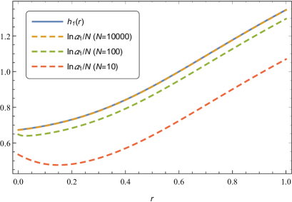
Figure 1: The plots of functions for $u=0.4$, showing the validity of the asymptotic behavior. It is seen that as $N$ becomes large, $\ln{\alpha_{1}}/N\sim h_{1}$, meaning that $\alpha_{1}\sim e^{Nh_{1}}$. Since $\alpha_{2}(r)=\alpha_{1}(1-r)$, the asymptotic behavior of $\alpha_{2}$ is given by $e^{Nh_{1}(1-r)}=e^{Nh_{2}(r)}$.

Fig. 2 shows the behaviors of $h_{1}(r)$ and $h_{2}(u)$. From this figure, one can see that $\alpha_{1}\sim\alpha_{2}$ only when $r=1/2$ for $u\in(0,1/2)$.

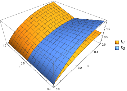
Figure 2: The comparison of $h_{1}$ and $h_{2}$. This plot shows that $h_{1}=h_{2}$ only if $r=1/2$ for $u\in(0,1/2)$.

$\beta$s are also obtained in the same way, and the results are

$$\begin{split}\beta_{1}&=\sum_{\begin{subarray}{c}k,l_{1},l_{2}\geq 0\\ k+l_{1}+l_{2}=K\end{subarray}}\frac{N!}{l_{1}!^{2}l_{2}!^{2}k!(N-2K+k)!}(r^{2}+(1-r)^{2})^{2k}r^{4l_{1}}(1-r)^{4l_{2}},\\ \beta_{2}&=\frac{1}{d_{S}}\alpha_{1}^{2},\\ \beta_{3}&=\frac{1}{d_{S}}\alpha_{1}\alpha_{2},\\ \beta_{4}&=\frac{1}{d_{S}}\alpha_{2}^{2},\\ \beta_{5}&=\sum_{\begin{subarray}{c}k,l_{1},l_{2}\geq 0\\ k+l_{1}+l_{2}=K\end{subarray}}\frac{N!}{l_{1}!^{2}l_{2}!^{2}k!(N-2K+k)!}\left(r^{2}+(1-r)^{2}\right)^{2k}r^{2(l_{1}+l_{2})}(1-r)^{2(l_{1}+l_{2})}.\end{split}$$ (40)

In this form, it might seem to be difficult to compare $\beta_{1}$ and $\beta_{5}$ with $\alpha_{1}^{2}$ and $\alpha_{2}^{2}$. However, as is derived in Appendix B, $|\beta_{1}|\leq|\alpha_{2}|^{2}$ and $|\beta_{5}|\leq|\beta_{4}|$ hold for any channel. Furthermore, if we interchange $r$ into $1-r$, $\alpha_{2}$ turns into $\alpha_{1}$ while $\beta_{1}$ is invariant. Thus, $|\beta_{1}|\leq\min_{i,j=1,2}{\{|\alpha_{i}\alpha_{j}|\}}$.

Since the asymptotic behaviors of $\alpha$s coincide with each other only when $r=1/2$, $|\beta_{1}|/\max_{i,j=1,2}{\{|\alpha_{i}\alpha_{j}|\}}$ is exponentially small except for $r=1/2$. For $r=1/2$, $\beta_{1}(1/2)=\beta_{5}(1/2)\leq\beta_{4}(1/2)=\alpha_{2}^{2}/d_{S}$. Therefore, the ratio of $\max_{u=1,\cdots,5}\{{|\beta_{u}|}\}$ to $\max_{i,j=1,2}{\{|\alpha_{i}\alpha_{j}|\}}$ is exponentially small for any $r\in[0,1]$, meaning that we have proven the following theorem:

Theorem 2.

Consider an $N$-qubit system $A$, where the energy difference between the excited state and the ground state is the same for each qubit. Under the assumption that the system is initially in a random pure state in an energy shell and that each qubit evolves according to the amplitude damping channel, the second Rényi entropy between the system $A$ and its environment is typical when $N\to\infty$.

It would be interesting to compare the typical value with the Page-like curve for the second Rényi entropy. The total energy for the $N$-qubit system is $E(r)=Nu\omega(1-r)$. The corresponding Gibbs state is given by

$$\rho_{\mathrm{Gibbs}}(r)=\bigotimes_{n=1}^{N}\left(u(1-r)\ket{+}_{n}\bra{+}_{n}+\left(1-u(1-r)\right)\ket{-}_{n}\bra{-}_{n}\right).$$ (41)

The second Rényi entropy per qubit defined by

$$\frac{1}{N}R_{2}^{\mathrm{thermal}}(r)\equiv-\frac{1}{N}\ln{\left(\mathrm{Tr}\left(\rho_{\mathrm{Gibbs}}{}_{,u}(r)^{2}\right)\right)}=-\ln{\left(u^{2}(1-r)^{2}+\left(1-u(1-r)\right)^{2}\right)}.$$ (42)

satisfies

$$\frac{1}{N}R_{2}^{\mathrm{thermal}}(r=1)=0,\quad\frac{d}{dr}\left(\frac{1}{N}R_{2}^{\mathrm{thermal}}(r)\right)\Biggr{|}_{r=1}=-2u,$$ (43)

where $r=1$ is the complete evaporation point. On the other hand,

$$\frac{1}{N}\tilde{R}_{2}(r=1)=0,\quad\frac{d}{dr}\left(\frac{1}{N}\tilde{R}_{2}(r)\right)\Biggr{|}_{r=1} \sim-\frac{d}{dr}h_{1}(r)\Biggr{|}_{r=1}=-2u.$$ (44)

Therefore, at the very last stage of the dissipation process, the Page curve-like behavior is reproduced. Fig. 3 shows the comparison of $R_{2}^{\mathrm{thermal}}$ and $\tilde{R}_{2}$ for $r\in[0,1]$.

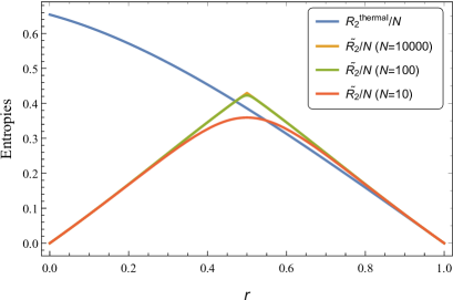
Figure 3: Comparison of the typical behavior of the second Rényi entropy and the thermal Rényi entropy for $u=0.4$. At the very last stage of the dissipation process, i.e., $r\approx 1$, $\tilde{R}_{2}\approx R_{2}^{\mathrm{thermal}}$, meaning that the Page curve-like behavior is reproduced.

III.2 Arbitrary single-qudit process with trivial free Hamiltonian

In the previous subsection, it has been shown that the second Rényi entropy has a typical behavior for a dissipating qubit system whose dynamics is described by the multiple-product of the amplitude damping channel. Then, a natural question arises: is the typicality specific to the energy-dissipating process? In this subsection, it is proven that for any channel composed of a multiple-product of a single-qudit quantum channel, $R_{2}$ has a typical behavior if the initial state is randomly chosen from the whole Hilbert space, i.e., $\mathcal{H}_{S}=\mathcal{H}_{A}$. This choice of the initial state corresponds to the microcanonical ensemble for a system $A$ with the trivial free Hamiltonian $H=0$ or at infinite temperature. Although this set up may not corresponds to a realistic system, the important implication is that for a wide range of dynamics, there may be a corresponding typical entanglement.

When $\mathcal{H}_{S}=\mathcal{H}_{A}$, $P=\mathbb{I}_{\mathcal{H}_{A}}$ and $R_{\mu}=Q_{\mu}$. Let us introduce an orthonormal basis $\sigma_{\mu}^{(1\text{-qudit})}$ for the set of linear operators on a single-qudit system. A basis can be constructed by $\sigma_{\mu}\equiv\bigotimes_{n=1}^{N}\sigma_{\mu_{n}}^{(1\text{-qudit})}$, where we have identified $\mu=0,\cdots,d^{N}-1$ with its $N$-length $d$-ary representation $\mu=\mu_{1}\mu_{2}\cdots\mu_{N}$. Assuming $\mathcal{E}_{A}=\mathcal{E}^{\otimes N}$ for some single-qudit quantum channel $\mathcal{E}$, $Q_{\mu}=\bigotimes_{n=1}^{N}Q_{\mu_{n}}^{(1\text{-qudit})}$, where we have defined

$$Q_{\mu}^{(1\text{-qudit})}\equiv\sum_{i}K_{i}^{\dagger}\sigma_{\mu}^{(1\text{-qudit})}K_{i}$$ (45)

by using a set of Kraus operators $\{K_{i}\}$ of the channel $\mathcal{E}$. Therefore, $\alpha_{i}=a_{i}^{N}$ and $\beta_{u}=b_{u}^{N}$ holds for $i=1,2$ and $u=1,\cdots,5$, where

$$a_{1}\equiv\sum_{\mu=0}^{d^{2}-1}\mathrm{Tr}\left(Q_{\mu}^{(1\text{-qudit})}\right)^{2},\quad a_{2}\equiv\sum_{\mu=0}^{d^{2}-1}\mathrm{Tr}\left(\left(Q_{\mu}^{(1\text{-qudit})}\right)^{2}\right),$$ (46)

and

$$\begin{split}b_{1}&\equiv\sum_{\mu=0}^{d^{2}-1}\sum_{\nu=0}^{d^{2}-1}\left(\mathrm{Tr}\left(Q_{\mu}^{(1\text{-qudit})}Q_{\nu}^{(1\text{-qudit})}\right)\right)^{2},\\ b_{2}&\equiv\sum_{\mu=0}^{d^{2}-1}\sum_{\nu=0}^{d^{2}-1}\mathrm{Tr}\left(Q_{\mu}^{(1\text{-qudit})}Q_{\nu}^{(1\text{-qudit})}\right)\mathrm{Tr}\left(Q_{\mu}^{(1\text{-qudit})}\right)\mathrm{Tr}\left(Q_{\nu}^{(1\text{-qudit})}\right),\\ b_{3}&\equiv\sum_{\mu=0}^{d^{2}-1}\sum_{\nu=0}^{d^{2}-1}\mathrm{Tr}\left(Q_{\mu}^{(1\text{-qudit})}\left(Q_{\nu}^{(1\text{-qudit})}\right)^{2}\right)\mathrm{Tr}\left(Q_{\mu}^{(1\text{-qudit})}\right),\\ b_{4}&\equiv\sum_{\mu=0}^{d^{2}-1}\sum_{\nu=0}^{d^{2}-1}\mathrm{Tr}\left(\left(Q_{\mu}^{(1\text{-qudit})}\right)^{2}\left(Q_{\nu}^{(1\text{-qudit})}\right)^{2}\right),\\ b_{5}&\equiv\sum_{\mu=0}^{d^{2}-1}\sum_{\nu=0}^{d^{2}-1}\mathrm{Tr}\left(Q_{\mu}^{(1\text{-qudit})}Q_{\nu}^{(1\text{-qudit})}Q_{\mu}^{(1\text{-qudit})}Q_{\nu}^{(1\text{-qudit})}\right).\end{split}$$ (47)

Applying Theorem 1 for $\left\{Q_{\mu}^{(1\text{-qudit})}\right\}_{\mu=0}^{d^{2}-1}$, $\max_{u=1,\cdots,5}\{|b_{u}|\}<\max_{i,j=1,2}\{|a_{i}a_{j}|\}$ holds, which implies that the ratio of $\max_{u=1,\cdots,5}\{|\beta_{u}|\}$ to $\max_{i,j=1,2}\{|\alpha_{i}\alpha_{j}|\}$ is exponentially small in $N$. Therefore, we have established the following theorem:

Theorem 3.

Consider an $N$-qudit system $A$ whose time evolution is described by $\mathcal{E}^{\otimes N}$ for some single-qudit channel $\mathcal{E}$. Assuming the initial pure state is randomly chosen from the whole Hilbert space, the second Rényi entropy between the system $A$ and its environment is typical when $N\to\infty$.

As an example, let us consider the phase damping channel defined by Kraus operators $K_{1}\equiv\ket{+}\bra{+}+\sqrt{1-\lambda}\ket{-}\bra{-}$ and $K_{2}\equiv\sqrt{\lambda}\ket{-}\bra{-}$ for an orthonormal basis $\{\ket{+},\ket{-}\}$ and $\lambda\in[0,1]$. This channel describes an information-loss process without loss of energy. As is easily calculated, $a_{1}=2$ and $a_{2}=2(2-\lambda)$. Thus, $\tilde{R}_{2}=-\ln{\left((2^{N}+2^{N}(2-\lambda)^{N})/(2^{N}(2^{N}+1))\right)}$. The plot of $\tilde{R}_{2}$ is given in Fig. 4, showing a qualitatively different behavior from Page-like curves.

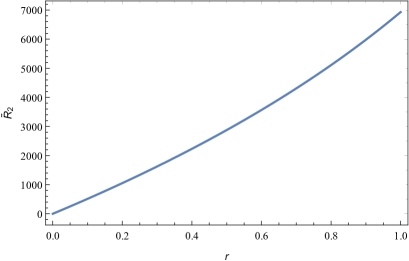
Figure 4: The plot of $\tilde{R}_{2}$ in the phase damping channel for $N=10000$. Since the phase damping channel suppresses the off-diagonal component of the initial state, the system $A$ becomes more entangled with its environment as $\lambda$ becomes large. This behavior is qualitatively different from the energy dissipation process described by the amplitude damping channel, where the entropy starts to decrease at some point.

IV Conclusions

In this paper, we investigated the typicality of entanglement for dynamical processes. To investigate the typicality of the $m$-th Rényi entropy, we have obtained a formula to calculate the average and the variance for the trace of $m$-th power of a state. For a normal thermodynamical system initially prepared according to the microcanonical ensemble, the ratio of $\max_{u}\{|\beta_{u}|\}$ to $\max_{i,j}\{|\alpha_{i}\alpha_{j}|\}$ gives an important criterion for the typicality of the second Rényi entropy. We presented two analytically tractable cases where the second Rényi entropy has a typical behavior. The first one was an energy dissipation process in a multiple-qubit system, whose typical entanglement is qualitatively similar to a Page-like curve. This gives the “first proof” of the Page curve conjecture as a dynamical process. In the second case, a multiple-qudit system was initially prepared as a pure state randomly chosen from the whole Hilbert space. It was shown that for dynamics described by a multiple-product of a single-qudit quantum channel, there is a typical behavior of the second Rényi entropy. This result implies that the typicality is not a specific feature of a energy dissipation process.

The formula for the average and the variance serived in Section II is applicable for any dynamics and distribution of the initial state, while it is difficult to obtain their asymptotic behaviors. It is still an open question when entanglement has a typical behavior in general. It will be also interesting to investigate the typicality of higher order Rényi entropy in future research. Once one could show typicality for all orders of Rényi entropy, the typical behavior of the entanglement entropy can be obtained from the analytical continuation.

Appendix A Formula for the formula for ensemble average

Theorem 4.

For any orthonormal basis $\left\{\ket{i}\right\}_{i=1}^{d_{S}}$ of $\mathcal{H}_{S}$ and the coefficients for a Haar-random pure state $\ket{\Psi}\equiv\sum_{i}X_{i}\ket{i}\in\mathcal{H}$ and a positive integer $m$,

$$\overline{\prod_{k=1}^{m}X_{i^{(k)}}X_{j^{(k)}}{}^{*}}=\frac{\Gamma(d_{S})}{\Gamma(d_{S}+m)}\sum_{\tau\in S_{m}}\prod_{k=1}^{m}\delta_{j^{(k)},i^{(\tau(k))}}$$ (48)

, where the overline denotes the integration over the Haar measure for the unitary group on $\mathcal{H}_{S}$, $S_{m}$ is the symmetric group of degree $m$ and $d_{S}\equiv\dim{\mathcal{H}_{S}}$.

Proof.

Any pure state in $\mathcal{H}_{S}$ can be written as $\ket{\Psi}=U\ket{0}=\sum_{i}U_{i,0}\ket{i}$ , where $\ket{0}\in\mathcal{H}_{S}$ is a unit vector, $U$ is a unitary operator and $U_{i,0}\equiv\braket{i}{U}{0}$. Taking $U$ as random, we get a random pure state $\ket{\Psi}$.

From the Weingarten calculus formula Collins , we have

$$\overline{\prod_{k=1}^{m}U_{i^{(k)},j^{(k)}}U_{i^{(k)^{\prime}},j^{(k)^{\prime}}}{}^{*}}=\sum_{\tau_{1},\tau_{2}\in S_{m}}\prod_{k=1}^{m}\delta_{i^{(k)^{\prime}},i^{(\tau_{1}(k))}}\delta_{j^{(k)^{\prime}},j^{(\tau_{2}(k))}}\mathrm{Wg}_{d_{S}}(\tau_{2}\tau_{1}^{-1})$$

, where $\mathrm{Wg}_{d_{S}}(\tau_{2}\tau_{1}^{-1})$ is called the Weingarten function, which depend on $d_{S}$ and $\tau_{2}\tau_{1}^{-1}$. Here we do not need any detail of this function. In the case of random pure state, this formula is simplified as follows:

$$\overline{\prod_{k=1}^{m}U_{i^{(k)},0}U_{i^{(k)^{\prime}},0}{}^{*}} =\sum_{\tau_{1},\tau_{2}\in S_{m}}\prod_{k=1}^{m}\delta_{i^{(k)^{\prime}},i^{(\tau_{1}(k))}}\mathrm{Wg}_{d_{S}}(\tau_{2}\tau_{1}^{-1})$$

$$=c\sum_{\tau\in S_{m}}\prod_{k=1}^{m}\delta_{i^{(k)^{\prime}},i^{(\tau(k))}}$$

, where we have defined $c\equiv\sum_{\tau\in S_{m}}\mathrm{Wg}_{d_{S}}(\tau)$. For notational convenience, let us write $X_{i}\equiv U_{i,0}$. Then, a Haar-random state is written as $\ket{\Psi}=\sum_{i}X_{i}\ket{i}$ and $X_{i}$ satisfies

$$\overline{\prod_{k=1}^{m}X_{i^{(k)}}X_{i^{(k)^{\prime}}}{}^{*}}=c\sum_{\tau\in S_{m}}\prod_{k=1}^{m}\delta_{i^{(k)^{\prime}},i^{(\tau(k))}}$$

The coefficient $c$ is determined by the normalization condition of the Haar measure. To calculate $c$, let us consider $\mathrm{Tr}\left(\left(\ket{\Psi}\bra{\Psi}\right)^{m}\right)$. Since $\mathrm{Tr}\left(\left(\ket{\Psi}\bra{\Psi}\right)^{m}\right)=1$ holds for any pure state, we have

$$1 =\overline{1}=\overline{\mathrm{Tr}\left(\left(\ket{\Psi}\bra{\Psi}\right)^{m}\right)}=\overline{\prod_{k=1}^{m}\sum_{i^{(k)},i^{(k)^{\prime}}}X_{i^{(k)}}X_{i^{(k)^{\prime}}}{}^{*}\delta_{i^{(k)^{\prime}},i^{(k+1)}}}$$

$$=c\sum_{\tau\in S_{m}}\prod_{k=1}^{m}\sum_{i^{(k)},i^{(k)^{\prime}}}\delta_{i^{(k)^{\prime}},i^{(\tau(k))}}\delta_{i^{(k)^{\prime}},i^{(k+1)}}$$

$$=c\sum_{\tau\in S_{m}}\prod_{k=1}^{m}\sum_{i^{(k)},}\delta_{i^{(\tau(k))},i^{(k+1)}}=c\sum_{\tau\in S_{m}}\prod_{k=1}^{m}\sum_{i^{(k)},}\delta_{i^{(\sigma(k))},i^{(k)}}$$

$$=c\sum_{k=0}^{m}\begin{bmatrix}m\\ k\end{bmatrix}d_{S}^{k}=c\frac{\Gamma(d_{S}+m)}{\Gamma(d_{S})}$$

, where $\begin{bmatrix}m\\ k\end{bmatrix}$ is the unsigned Stirling numbers of the first kind, i.e. the number of elements in $S_{m}$ with $k$ disjoint cycle. Therefore,

$$c=\frac{\Gamma(d_{S})}{\Gamma(d_{S}+m)}$$

. ∎

Appendix B Proof of Theorem 1

Let us start with the following two lemmas:

Lemma 1.

For two positive matrices $M$, $N$, $\mathrm{Tr}\left(MN\right)\leq\mathrm{Tr}\left(M\right)\mathrm{Tr}\left(N\right)$ holds. The inequality holds as an equality if and only if one of the following conditions is satisfied:

1. $M=0$.

2. $N=0$.

3. $M=mP$ and $N=nP$ for some positive numbers $m,n$ and a one-dimensional projection operator $P$.

Proof.

By using the eigenvalue decompositions $M=\sum_{i}m_{i}\ket{m_{i}}\bra{m_{i}}$ and $N=\sum_{i}n_{i}\ket{n_{i}}\bra{n_{i}}$,

$$\mathrm{Tr}\left(MN\right)=\sum_{i,j}m_{i}n_{j}\left|\Braket{m_{i}}{n_{j}}\right|^{2},\quad\mathrm{Tr}\left(M\right)\mathrm{Tr}\left(N\right)=\sum_{i,j}m_{i}n_{j}.$$

Since $m_{i},n_{i}\geq 0$ and $\left|\braket{m_{i}}{n_{j}}\right|^{2}\leq 1$, $\mathrm{Tr}\left(MN\right)\leq\mathrm{Tr}\left(M\right)\mathrm{Tr}\left(N\right)$. The equality holds if and only if for any set of $(i,j)$, one of the following conditions is satisfied:

1. $m_{i}=0$.

2. $n_{j}=0$.

3. $\left|\braket{m_{i}}{n_{j}}\right|=1$.

If $M$ or $N$ is the zero operator, this condtion is satisfied. If $M$ and $N$ are not the zero operators, there exists a set of indices $(i_{0},j_{0})$ such that $m_{i_{0}}\neq 0$ and $n_{i_{0}}\neq 0$. Then $|\braket{m_{i_{0}}}{n_{j_{0}}}|=1$ holds, and

$$0=\braket{n_{j_{0}}}{n_{j_{0}}}-1=\sum_{i}|\braket{m_{i}}{n_{j_{0}}}|^{2}-1=\sum_{i\neq i_{0}}|\braket{m_{i}}{n_{j_{0}}}|^{2},$$ (49)

which implies $m_{i}=0$ for all $i\neq i_{0}$. Similarly, $n_{j}=0$ for all $j\neq j_{0}$. Therefore, $M=m_{i_{0}}P$ and $N=n_{j_{0}}P$, where $P\equiv\ket{m_{i_{0}}}\bra{m_{i_{0}}}=\ket{n_{j_{0}}}\bra{n_{j_{0}}}$ is a one-dimensional projection operator. ∎

Lemma 2.

For any set of real numbers $\{r_{i}\}_{i=1}^{n}$ and Hermite operators $\{R_{i}\}_{i=1}^{n}$, it holds

$$\mathrm{Tr}\left(\left(\sum_{i=1}^{n}r_{i}R_{i}\right)^{2}\right)\leq\left(\sum_{i=1}^{n}r_{i}^{2}\right)\left(\sum_{j=1}^{n}\mathrm{Tr}(R_{j}^{2})\right).$$ (50)

The inequality holds as an equality if and only if there exists an Hermite operator $A$ such that for all $i=1,2,\cdots n$, $R_{i}=r_{i}A$.

Proof.

Define an orthonormal basis $\{\sigma_{\mu}\}_{\mu}$ for a set of Hermite operators, satisfying $\mathrm{Tr}\left(\sigma_{\mu}\sigma_{\nu}\right)=\delta_{\mu,\nu}$. The Hermite operators can be expanded as $R_{i}=\sum_{\mu}c_{i,\mu}\sigma_{\mu}$ by using coefficients $c_{i,\mu}\in\mathbb{R}$. By using the Cauchy–Schwartz inequality, we get

$$\mathrm{Tr}\left(\left(\sum_{i=1}^{n}r_{i}R_{i}\right)^{2}\right) =\sum_{\mu}\left(\sum_{i=1}^{n}r_{i}c_{i,\mu}\right)^{2}$$

$$\leq\sum_{\mu}\left(\sum_{i=1}^{n}r_{i}^{2}\right)\left(\sum_{j=1}^{n}c_{j,\mu}^{2}\right)=\left(\sum_{i=1}^{n}r_{i}^{2}\right)\left(\sum_{j=1}^{n}\mathrm{Tr}(R_{j}^{2})\right).$$ (51)

The equality holds if and only if for all $\mu$, there exists a real number $k_{\mu}$ such that $c_{i,\mu}=k_{\mu}r_{i}$ for $i=1,2,\cdots,n$, i.e., $R_{i}=\sum_{\mu}c_{i,\mu}\sigma_{\mu}=r_{i}A$, where $A\equiv\sum_{\mu}k_{\mu}\sigma_{\mu}$ is an Hermite operator. ∎

By using Lemma 1 and 2, the following theorem is proved:

Theorem 5.

For any set of Hermite operators $\{R_{\mu}\}_{\mu}$, the following inequality holds:

$$\max_{i,j}\left\{|\alpha_{i}\alpha_{j}|\right\}\geq\max_{u}\left\{|\beta_{u}|\right\},$$ (52)

where

$$\alpha_{1} \equiv\sum_{\mu}\mathrm{Tr}\left(R_{\mu}\right)^{2},\,\alpha_{2}\equiv\sum_{\mu}\mathrm{Tr}\left(R_{\mu}^{2}\right),$$

$$\beta_{1} \equiv\sum_{\mu,\nu}\left(\mathrm{Tr}\left(R_{\mu}R_{\nu}\right)\right)^{2},\,\beta_{2}\equiv\sum_{\mu,\nu}\mathrm{Tr}\left(R_{\mu}R_{\nu}\right)\mathrm{Tr}\left(R_{\mu}\right)\mathrm{Tr}\left(R_{\nu}\right),$$

$$\beta_{3} \equiv\sum_{\mu,\nu}\mathrm{Tr}\left(R_{\mu}R_{\nu}^{2}\right)\mathrm{Tr}\left(R_{\mu}\right),\,\beta_{4}\equiv\sum_{\mu,\nu}\mathrm{Tr}\left(R_{\mu}^{2}R_{\nu}^{2}\right),\,\beta_{5}\equiv\sum_{\mu,\nu}\mathrm{Tr}\left(R_{\mu}R_{\nu}R_{\mu}R_{\nu}\right).$$

The inequality holds as an equality if and only if there exists an Hermite operator $A$ satisfying $\mathrm{Tr}\left(A^{2}\right)\geq\mathrm{Tr}\left(A\right)^{2}$ such that $\forall\mu$, $\exists r_{\mu}\in\mathbb{R}$, $R_{\mu}=r_{\mu}A$.

Proof.

Without loss of generality, one can assume $R_{\mu}\neq 0$ for all $\mu$ since a zero operator does not contribute all $\alpha$s and $\beta$s. Let us consider an upperbound for each $\beta_{u}$ one by one.

• $\beta_{1}=\sum_{\mu,\nu}\left(\mathrm{Tr}\left(R_{\mu}R_{\nu}\right)\right)^{2}$:
  For any set of $(\mu,\nu)$,

  $$\left(\mathrm{Tr}\left(R_{\mu}R_{\nu}\right)\right)^{2}\leq\mathrm{Tr}\left(R_{\mu}^{2}\right)\mathrm{Tr}\left(R_{\nu}^{2}\right),$$ (53)

  where we have used the Cauchy-Schwartz inequality for the Hilbert–Schmidt inner product. The inequality holds as an equality if and only if $\exists\alpha\indices{{}_{\mu}^{\nu}}\in\mathbb{R}$ s.t. $R_{\mu}=\alpha\indices{{}_{\mu}^{\nu}}R_{\nu}$. Since $R_{\mu}\neq 0$ for all $\mu$, $\exists r_{\mu}\in\mathbb{R}\backslash\{0\}$ s.t. $R_{\mu}=r_{\mu}A$ for some Hermite operator $A$. Then, $\left(\mathrm{Tr}\left(R_{\mu}\right)\right)^{2}=r_{\mu}^{2}\left(\mathrm{Tr}\left(A\right)\right)^{2}$ and $\mathrm{Tr}\left(R_{\mu}^{2}\right)=r_{\mu}^{2}\mathrm{Tr}\left(A^{2}\right)$. $\sum_{\mu,\nu}\mathrm{Tr}\left(R_{\mu}^{2}\right)\mathrm{Tr}\left(R_{\nu}^{2}\right)=\max_{i,j}\left\{|\alpha_{i}\alpha_{j}|\right\}$ if and only if $\mathrm{Tr}\left(R_{\mu}^{2}\right)\geq\left(\mathrm{Tr}\left(R_{\mu}\right)\right)^{2}$, or equivalently $r_{\mu}^{2}(\mathrm{Tr}\left(A^{2}\right)-\mathrm{Tr}\left(A\right)^{2})\geq 0$ holds for all $\mu$. Thus, $\mathrm{Tr}\left(A^{2}\right)\geq\mathrm{Tr}\left(A\right)^{2}$.

• $\beta_{2}=\sum_{\mu,\nu}\mathrm{Tr}\left(R_{\mu}R_{\nu}\right)\mathrm{Tr}\left(R_{\mu}\right)\mathrm{Tr}\left(R_{\nu}\right)$:
  By using Lemma 2,

  $$\sum_{\mu,\nu}\mathrm{Tr}\left(R_{\mu}R_{\nu}\right)\mathrm{Tr}\left(R_{\mu}\right)\mathrm{Tr}\left(R_{\nu}\right)=\mathrm{Tr}\left(\left(\sum_{\mu}\mathrm{Tr}\left(R_{\mu}\right)R_{\mu}\right)^{2}\right)\leq\sum_{\mu,\nu}\mathrm{Tr}\left(R_{\mu}\right)^{2}\mathrm{Tr}\left(R_{\nu}^{2}\right).$$ (54)

  This inequality holds as an equality if and only if there exist an Hermite operator $A$ s.t. $R_{\mu}=\mathrm{Tr}\left(R_{\mu}\right)A$ for all $\mu$. Since we have assumed $R_{\mu}\neq 0$, this conditioin implies $\mathrm{Tr}\left(A\right)=1$. Noting $\sum_{\mu,\nu}\mathrm{Tr}\left(R_{\mu}\right)^{2}\mathrm{Tr}\left(R_{\nu}^{2}\right)(=\alpha_{1}\alpha_{2})=\max_{i,j}\left\{|\alpha_{i}\alpha_{j}|\right\}$ if and only if $\sum_{\mu}\mathrm{Tr}\left(R_{\mu}^{2}\right)=\sum_{\mu}\mathrm{Tr}\left(R_{\mu}\right)^{2}$, it follows that $\mathrm{Tr}\left(A^{2}\right)=1(=\mathrm{Tr}\left(A\right)^{2})$.

• $\beta_{3}=\sum_{\mu,\nu}\mathrm{Tr}\left(R_{\mu}R_{\nu}^{2}\right)\mathrm{Tr}\left(R_{\mu}\right)$:
  By using the Cauchy–Schwartz inequality,

  $$\left|\sum_{\mu,\nu}\mathrm{Tr}\left(R_{\mu}R_{\nu}^{2}\right)\mathrm{Tr}\left(R_{\mu}\right)\right| =\left|\sum_{\mu}\mathrm{Tr}\left(R_{\mu}\sum_{\nu}R_{\nu}^{2}\right)\mathrm{Tr}\left(R_{\mu}\right)\right|$$

  $$\leq\sqrt{\sum_{\mu}\left(\mathrm{Tr}\left(R_{\mu}\right)\right)^{2}\sum_{\rho}\left(\mathrm{Tr}\left(R_{\rho}\sum_{\nu}R_{\nu}^{2}\right)\right)^{2}}.$$ (55)

  By using the Cauchy–Schwartz inequality,

  $$\left(\mathrm{Tr}\left(R_{\rho}\sum_{\nu}R_{\nu}^{2}\right)\right)^{2} \leq\mathrm{Tr}\left(\left(\sum_{\nu}R_{\nu}^{2}\right)^{2}\right)\mathrm{Tr}\left(R_{\rho}^{2}\right)=\sum_{\mu,\nu}\mathrm{Tr}\left(R_{\mu}^{2}R_{\nu}^{2}\right)\mathrm{Tr}\left(R_{\rho}^{2}\right)$$

  $$\leq\sum_{\mu,\nu}\mathrm{Tr}\left(R_{\mu}^{2}\right)\mathrm{Tr}\left(R_{\nu}^{2}\right)\mathrm{Tr}\left(R_{\rho}^{2}\right)$$ (56)

  holds for all $\rho$. On the second line, we have used Lemma 1. The second inequality holds as an equality if and only if $R_{\mu}=r_{\mu}P$ for some $r_{\mu}\in\mathbb{R}$ and a one-dimensional projector $P$. Thus,

  $$\left|\sum_{\mu,\nu}\mathrm{Tr}\left(R_{\mu}R_{\nu}^{2}\right)\mathrm{Tr}\left(R_{\mu}\right)\right| \leq\sqrt{\left(\sum_{\mu}\left(\mathrm{Tr}\left(R_{\mu}\right)\right)^{2}\right)\left(\sum_{\nu}\mathrm{Tr}\left(R_{\nu}^{2}\right)\right)^{3}}$$

  $$\leq\max{\left\{\alpha_{1}^{2},\alpha_{2}^{2}\right\}}.$$ (57)

• $\beta_{4}=\sum_{\mu,\nu}\mathrm{Tr}\left(R_{\mu}^{2}R_{\nu}^{2}\right)$
  Since $R_{\nu}^{2}$ is a positive operator,

  $$\mathrm{Tr}\left(R_{\mu}^{2}R_{\nu}^{2}\right)\leq\mathrm{Tr}\left(R_{\mu}^{2}\right)\mathrm{Tr}\left(R_{\nu}^{2}\right).$$ (58)

  Since we have assuumed $R_{\mu}\neq 0$, the inequality holds as an equality for any pair of $(\mu,\nu)$ if and only if there exists one-dimensional projection operator $P$ s.t. $\forall\mu$, $\exists a_{\mu}\in\mathbb{R}_{>0}$ s.t. $R_{\mu}^{2}=a_{\mu}P$. This condition is equivalent to $R_{\mu}=r_{\mu}P$, where $r_{\mu}=\pm\sqrt{a_{\mu}}$.

• $\beta_{5}=\sum_{\mu,\nu}\mathrm{Tr}\left(R_{\mu}R_{\nu}R_{\mu}R_{\nu}\right)$
  By using a commutator defined by $\left[A,B\right]\equiv AB-BA$,

  $$\mathrm{Tr}\left(R_{\mu}R_{\nu}R_{\mu}R_{\nu}\right) =\mathrm{Tr}\left(R_{\mu}^{2}R_{\nu}^{2}\right)+\mathrm{Tr}\left(R_{\mu}R_{\nu}\left[R_{\mu},R_{\nu}\right]\right)$$ (59)

  holds. Since $i\left[Q_{\mu},Q_{\nu}\right]$ is Hermite,

  $$\sum_{\mu,\nu}\mathrm{Tr}\left(R_{\mu}R_{\nu}\left[R_{\mu},R_{\nu}\right]\right)=-\frac{1}{2}\sum_{\mu,\nu}\mathrm{Tr}\left(\left(i\left[R_{\mu},R_{\nu}\right]\right)^{2}\right)\leq 0.$$ (60)

  Thus,

  $$\sum_{\mu,\nu}\mathrm{Tr}\left(R_{\mu}R_{\nu}R_{\mu}R_{\nu}\right)\leq\sum_{\mu,\nu}\mathrm{Tr}\left(R_{\mu}^{2}R_{\nu}^{2}\right).$$ (61)

  By using anticommutator $\left\{A,B\right\}\equiv AB+BA$, a similar calculation shows

  $$\mathrm{Tr}\left(R_{\mu}R_{\nu}R_{\mu}R_{\nu}\right)=-\mathrm{Tr}\left(R_{\mu}^{2}R_{\nu}^{2}\right)+\mathrm{Tr}\left(R_{\mu}\left\{R_{\mu},R_{\nu}\right\}R_{\nu}\right)$$ (62)

  and

  $$\sum_{\mu,\nu}\mathrm{Tr}\left(R_{\mu}\left\{R_{\mu},R_{\nu}\right\}R_{\nu}\right)=\frac{1}{2}\sum_{\mu,\nu}\mathrm{Tr}\left(\left\{R_{\mu},R_{\nu}\right\}^{2}\right)\geq 0,$$ (63)

  which implies

  $$\sum_{\mu,\nu}\mathrm{Tr}\left(R_{\mu}R_{\nu}R_{\mu}R_{\nu}\right)\geq-\sum_{\mu,\nu}\mathrm{Tr}\left(R_{\mu}^{2}R_{\nu}^{2}\right).$$ (64)

  Therefore, $|\beta_{5}|\leq|\beta_{4}|$.

∎

Let us define a set of operators $\{R_{\mu}\}_{\mu}$ as $R_{\mu}\equiv P\left(\sum_{i}K_{i}^{\dagger}\sigma_{\mu}K_{i}\right)P$ by using a set of Kraus operators $\{K_{i}\}_{i}$ and a projection operator $P$ onto the sub-Hilbert space $\mathcal{H}_{S}$. Since Kraus operators satisfy $\sum_{i}K_{i}^{\dagger}K_{i}=\mathbb{I}_{\mathcal{H}_{A}}$, we get $R_{0}=\frac{1}{\sqrt{d_{A}}}P\mathbb{I}_{A}P=\frac{1}{\sqrt{d_{A}}}P$. Assume the equality in Eq. (52) holds, then $A=kP$ for some $k\in\mathbb{R}\backslash\{0\}$. Since $\mathrm{Tr}\left(A^{2}\right)=k^{2}d_{S}$ and $\mathrm{Tr}\left(A\right)^{2}=k^{2}d_{S}^{2}$, the conditioin $\mathrm{Tr}\left(A^{2}\right)\geq\mathrm{Tr}\left(A\right)^{2}$ implies $d_{S}=1$, which concludes the proof of Theorem 1.

Appendix C The asymptotic behavior of the Hypergeometric function

In this section, we derive the asymptotic behavior of the Hypergeometric function ${}_{2}F_{1}\left(-uN,-uN;(1-2u)N+1;z\right)$ for $u\in[0,1/2)$. It is known that the Hypergeometric function ${}_{2}F_{1}\left(a,b;c;z\right)$ is the solution for the following differential equation satisfying $f(z=0)=1$:

$$z(1-z)\frac{d^{2}}{dz^{2}}f+(c-(a+b+1)z)\frac{d}{dz}f-abf=0.$$ (65)

Defining a function $g(z)\equiv\frac{1}{N}\ln{f(z)}$, we get

$$f^{-1}\frac{d}{dz}f(z)=N\frac{d}{dz}g(z),\quad f^{-1}\frac{d^{2}}{dz^{2}}f(z)=\left(N\frac{d}{dz}g(z)\right)^{2}+N\frac{d^{2}}{dz^{2}}g(z).$$ (66)

Therefore, for $N\gg 1$, $g(z)$ satisfies

$$z(1-z)\left(\frac{d}{dz}g(z)\right)^{2}+(\gamma-(\alpha+\beta)z)\frac{d}{dz}g-\alpha\beta=0,$$ (67)

where we have assumed $a,b,c\in\mathbb{R}$ and they have the form of $a=\alpha N+a^{\prime}$, $b=\beta N+b^{\prime}$ and $c=\gamma N+c^{\prime}$ with $N$-independent constants $a^{\prime},\,b^{\prime},\,c^{\prime},\,\alpha,\,\beta$, and $\gamma$. Then, $\frac{d}{dz}g(z)$ satisfies

$$\frac{d}{dz}g(z) =\frac{-(\gamma-(\alpha+\beta)z)\pm\sqrt{\left(\gamma-(\alpha+\beta)z\right)^{2}+4\alpha\beta z(1-z)}}{2z(1-z)}$$

$$=\frac{-(\gamma-(\alpha+\beta)z)\pm|\gamma|\sqrt{1+sz+tz^{2}}}{2z(1-z)},$$ (68)

where we have defined $s\equiv\frac{4\alpha\beta-2\gamma(\alpha+\beta)}{\gamma^{2}}$ and $t\equiv\frac{(\alpha-\beta)^{2}}{\gamma^{2}}$. One can confirm that

$$\frac{\sqrt{1+sz+tz^{2}}}{z(1-z)} =\frac{\sqrt{1+s+t}}{1-z}+\frac{1}{z}-\frac{s+\frac{s+2tz}{\sqrt{1+sz+tz^{2}}}}{2+sz+2\sqrt{1+sz+tz^{2}}}-\sqrt{t}\frac{\left(2t+\frac{\sqrt{t}\left(s+2tz\right)}{\sqrt{1+sz+tz^{2}}}\right)}{s+2tz+2\sqrt{t}\sqrt{1+sz+tz^{2}}}$$

$$\qquad\qquad+\frac{\sqrt{1+s+t}\left(s+2t+\frac{\sqrt{1+s+t}\left(s+2tz\right)}{\sqrt{1+sz+tz^{2}}}\right)}{2+s+sz+2tz+2\sqrt{1+s+t}\sqrt{1+sz+tz^{2}}},$$ (69)

meaning that

$$\int dz\frac{\sqrt{1+sz+tz^{2}}}{z(1-z)}$$

$$=-\sqrt{1+s+t}\ln{\left(1-z\right)}+\ln{z}-\ln{\left(2+sz+2\sqrt{1+sz+tz^{2}}\right)}-\sqrt{t}\ln{\left(s+2tz+2\sqrt{t}\sqrt{1+sz+tz^{2}}\right)}$$

$$\qquad\qquad+\sqrt{1+s+t}\ln{\left(2+s+sz+2tz+2\sqrt{1+s+t}\sqrt{1+sz+tz^{2}}\right)}.$$ (70)

Imposing the boundary condition $g(z=0)=0$, we get

$$g(z)$$

$$=\frac{1}{2}\left(\gamma-(\alpha+\beta)-\gamma\sqrt{1+s+t}\right)\ln{\left(1-z\right)}$$

$$\qquad\qquad+\frac{\gamma}{2}\left(-\ln{\left(\frac{2+sz+2\sqrt{1+sz+tz^{2}}}{4}\right)}-\sqrt{t}\ln{\left(\frac{s+2tz+2\sqrt{t}\sqrt{1+sz+tz^{2}}}{s+2\sqrt{t}}\right)}\right.$$

$$\qquad\qquad\left.+\sqrt{1+s+t}\ln{\left(\frac{2+s+sz+2tz+2\sqrt{1+s+t}\sqrt{1+sz+tz^{2}}}{2+s+2\sqrt{1+s+t}}\right)}\right).$$ (71)

Since $\sqrt{1+s+t}=\left|\frac{\gamma-(\alpha+\beta)}{\gamma}\right|$, the divergent term at $z=1$ vanishes if $\frac{\gamma-(\alpha+\beta)}{\gamma}\geq 0$. For $\alpha=\beta=-u$ and $\gamma=1-2u$, $\frac{\gamma-(\alpha+\beta)}{\gamma}=\frac{1}{1-2u}>0$ holds for $u\in[0,1/2)$. Substituting $s=\frac{4u(1-u)}{(1-2u)^{2}}$ and $t=0$ into Eq. (71), ${}_{2}F_{1}\left(-uN,-uN;(1-2u)N+1;z\right)\sim\exp{\left(Ng_{u}(z)\right)}$ in the limit of $N\to\infty$, where

$$g_{u}(z) \equiv-\left(\frac{1}{2}-u\right)\ln{\left(\frac{2+\frac{4u(1-u)}{(1-2u)^{2}}z+2\sqrt{1+\frac{4u(1-u)}{(1-2u)^{2}}z}}{4}\right)}$$

$$\qquad\qquad+\frac{1}{2}\ln{\left(\frac{2+\frac{4u(1-u)}{(1-2u)^{2}}(1+z)+\frac{2}{1-2u}\sqrt{1+\frac{4u(1-u)}{(1-2u)^{2}}z}}{4\left(\frac{1-u}{1-2u}\right)^{2}}\right)}.$$ (72)

Since

$$\frac{2+\frac{4u(1-u)}{(1-2u)^{2}}(1+z)+\frac{2}{1-2u}\sqrt{1+\frac{4u(1-u)}{(1-2u)^{2}}z}}{4\left(\frac{1-u}{1-2u}\right)^{2}}>\frac{2+\frac{4u(1-u)}{(1-2u)^{2}}z+2\sqrt{1+\frac{4u(1-u)}{(1-2u)^{2}}z}}{4}$$ (73)

and $1/2-u<1/2$ holds for $u\in(0,1/2)$ and $z>0$, $g_{u}(z)>0$ holds, meaning that $\exp{\left(Ng_{u}(z)\right)}$ is exponentially large in $N$ for any $u\in(0,1/2)$ and $z>0$.

References

-
(1)
A. Sugita, On the Foundation of Quantum Statistical Mechanics (in Japanese), RIMS Kokyuroku (Kyoto) 1507, 147 (2006).
A. Sugita, On the Basis of Quantum Statistical Mechanics, Nonlinear Phenom. Complex Syst. 10, 192 (2007).
See also, S. Goldstein, J. L. Lebowitz, R. Tumulka, and N Zanghì, Canonical Typicality, Phys. Rev. Lett. 96, 050403 (2006). S. Popescu, A. J. Short, and A. Winter, Entanglement and the foundations of statistical mechanics, Nature Phys. 2, 754 (2006). - (2) H. Tasaki, Typicality of Thermal Equilibrium and Thermalization in Isolated Macroscopic Quantum Systems, J. Stat. Phys. 163, 5, 937 (2016).
- (3) J. L. Lebowitz, Boltzmann’s Entropy and Time’s Arrow, Physics Today 46, 9, 32 (1993).
- (4) J. M. Bardeen, B. Carter, and S. W. Hawking, The four laws of black hole mechanics, Commun. Math. Phys. 31, 161 (1973).
- (5) S. W. Hawking, Particle creation by black holes, Commun. Math. Phys. 43, 199 (1975).
- (6) See e.g., J. Bricmont, Science of Chaos or Chaos in Science?, Ann. of the New York academy of science, 775, 131 (1995).
- (7) E. Lubkin, Entropy of an n-system from its correlation with a k-reservoir, J. Math. Phys. 19, 1028 (1978).
- (8) S. Lloyd and H. Pagels, Complexity as thermodynamic depth, Ann. Phys. 188, 186 (1988).
- (9) D. N. Page, Average entropy of a subsystem, Phys. Rev. Lett. 71, 1291 (1993).
- (10) S. Sugiura and A. Shimizu, Canonical Thermal Pure Quantum State, Phys. Rev. Lett. 111, 010401 (2013).
- (11) H. Fujita, Y. O. Nakagawa, S. Sugiura, and M. Watanabe, Universality in volume-law entanglement of scrambled pure quantum states, Nature Commun. 9, 1635 (2018).
- (12) L. Vidmar, L. Hackl, E. Bianchi, and M. Rigol, Entanglement Entropy of Eigenstates of Quadratic Fermionic Hamiltonians, Phys. Rev. Lett. 119, 020601 (2017).
- (13) C. H. Bennett, P. W. Shor, J. A. Smolin, and A. V. Thapliyal, Entanglement-Assisted Classical Capacity of Noisy Quantum Channels, Phys. Rev. Lett. 83, 3081 (1999).
- (14) P. Calabrese and J. Cardy, Evolution of entanglement entropy in one-dimensional systems, J. Stat. Mech. 04, P04010 (2005).
- (15) J. M. Maldacena, The Large- Limit of Superconformal Field Theories and Supergravity, Adv. Theor. Math. Phys. 2, 231 (1998).
- (16) J. Bhattacharya, M. Nozaki, T. Takayanagi, and T. Ugajin, Thermodynamical Property of Entanglement Entropy for Excited States, Phys. Rev. Lett. 110, 091602 (2013).
- (17) M. Nozaki, T. Numasawa, A. Prudenziati, and T. Takayanagi, Dynamics of entanglement entropy from Einstein equation, Phys. Rev. D 88, 026012 (2013).
- (18) R. Fan, P. Zhang, H. Shen, and H. Zhai, Out-of-Time-Order Correlation for Many-Body Localization, Science Bulletin 62 (10), 707 (2017).
- (19) R. Islam, R. Ma, P. M. Preiss, M. E. Tai, A. Lukin, M. Rispoli, and M. Greiner, Measuring entanglement entropy in a quantum many-body system, Nature 528, 77, (2015).
- (20) A. M. Kaufman, M. E. Tai, A. Lukin, M. Rispoli, R. Schittko, P. M. Preiss, and M. Greiner, Quantum thermalization through entanglement in an isolated many-body system Science 353, 794 (2016).
- (21) S. W. Hawking, Breakdown of predictability in gravitational collapse, Phys. Rev. D 14, 2460 (1976).
- (22) M. Hotta, R. Schützhold, and W. G. Unruh, Partner particles for moving mirror radiation and black hole evaporation, Phys. Rev. D 91, 124060 (2015).
- (23) D. N. Page, Information in black hole radiation, Phys. Rev. Lett. 71, 3743 (1993).
- (24) A. Almheiri, D. Marolf, J. Polchinski, and J. Sully, Black holes: complementarity or firewalls?, J. High Energ. Phys. 02, 062 (2013).
- (25) A. Almheiri, D. Marolf, J. Polchinski, D. Stanford, and J. Sully, An apologia for firewalls, J. High Energ. Phys. 09, 18 (2013).
- (26) Y. Aharonov, A. Casher, and S. Nussinov, The unitarity puzzle and Planck mass stable particles, Phys. Lett. B 191, 51 (1987).
- (27) Z. Wilczek, Quantum purity at a small price: Easing a black hole paradox, in Proceedings of In- ternational Symposium in Houston on Black holes, membranes, wormholes and superstrings (1992), published in Blackholes, Membranes, Wormholes and Superstrings (edited by S. Kalara and DV Nanopoulos), World scientific, Singapore (1993).
- (28) W. G. Unruh and R. M. Wald, Information loss, Rep. Prog. Phys. 80, 092002 (2017).
- (29) S. W. Hawking, M. J. Perry, and A. Strominger, Soft Hair on Black Holes, Phys. Rev. Lett. 116, 231301 (2016).
- (30) J. D. Bekenstein, Black Holes and Entropy, Phys. Rev. D 7, 2333 (1973).
- (31) S. W. Hawking, Black holes and thermodynamics, Phys. Rev. D 13, 191 (1976).
- (32) M. Hotta, Y. Nambu, and K. Yamaguchi, Soft-hair-enhanced entanglement beyond Page curves in a black hole evaporation qubit model, Phys. Rev. Lett. 120, 181301 (2018).
- (33) B. Collins, Moments and Cumulants of Polynomial random variables on unitary groups, the Itzykson-Zuber integral and free probability, Int. Math. Res. Not. 17, 953 (2003).