Simultaneous Localization and Mapping with Dynamic Rigid Objects

Abstract

Accurate estimation of the environment structure simultaneously with the robot pose is a key capability of autonomous robotic vehicles. Classical simultaneous localization and mapping (SLAM) algorithms rely on the static world assumption to formulate the estimation problem, however, the real world has a significant amount of dynamics that can be exploited for a more accurate localization and versatile representation of the environment. In this paper we propose a technique to integrate the motion of dynamic objects into the SLAM estimation problem, without the necessity of estimating the pose or the geometry of the objects. To this end, we introduce a novel representation of the pose change of rigid bodies in motion and show the benefits of integrating such information when performing SLAM in dynamic environments. Our experiments show consistent improvement in robot localization and mapping accuracy when using a simple constant motion assumption, even for objects whose motion slightly violates this assumption.

I Introduction

Autonomous robotic platforms are rapidly departing from simple, controlled environments to more complex and dynamic ones. Self driving cars, mobile or flying robots in urban environments are only a few examples of emerging applications of robotic in dynamic environments. In order to perform tasks autonomously, a robot must be able to simultaneously build an accurate representation of the surroundings and localize itself. Simultaneous localization and mapping (SLAM) algorithms are a core enabling technology for autonomous mobile robotics.

SLAM is a well researched area in robotics, and many efficient solutions to the problem exist. However, the existing techniques heavily rely on the assumption that most parts of the environment are static [38]. Nevertheless, real world scenarios have a significant amount of dynamics that should not be discarded. The conventional technique for dealing with dynamic environment in SLAM is to either treat any feature associated with moving objects as outliers [13, 14, 41, 42, 45] or detect moving objects and track them separately using traditional multi-target tracking [39, 29, 30, 36]. However, ignoring dynamics in applications where the environment is cluttered with moving objects can cause the whole SLAM process to fail.

A typical SLAM system is composed of a front-end module, which processes the raw data from the sensors and a back-end module, which integrates the obtained information into a probabilistic framework. In visual SLAM, where cameras are the primary sensors for localization and mapping, simple primitives, such as point landmarks are commonly used to represent the environment. Points are easy to detect, track and integrate within the SLAM problem. Most of the existing methods assume that the dominant part of the scene changes only due to the camera motion, therefore they are prone to failure in highly dynamic environments. Other primitives such as lines and planes  [7, 22, 16, 18] and even objects  [31, 37] can provide richer map representations but they require higher level data processing.

Rapid advances in learning techniques for processing information from visual data, enable higher level sensing capabilities in robotic applications. Considerable effort has been devoted to developing accurate multi-object segmentation and tracking. Most of the existing techniques perform tracking only in the image-domain [43, 44], where pixels are labeled according to the object class they pertain to. In most of the cases, those methods require additional processing in order to be integrated into robotic applications  [37]. Other techniques use depth information obtained either from stereo cameras or LiDAR devices or scene geometry to track objects in 3D [26, 17]. In general, those methods require expensive point cloud processing, a priori models of the objects or even the known sensors locations.

In this paper, we propose a SLAM technique that can easily integrate information about the moving objects in the scene without the necessity of actually estimating the pose of the objects or relying on their 3D model. In particular, the formulation we propose uses the prior information that some of the structure points belong to moving objects, and the fact that these points can be associated in subsequent frames. In other words, it relies on a front-end able to identify and segment objects at image-level, associate points across the sequence of images and use semantic information to classify the feature points into either static or dynamic. It is worth mentioning that the problems of instance level object segmentation and data association are out of the scope of this paper, and considered as future work. The main contribution of this paper is the use of a novel pose change representation to model the motion of the points pertaining to rigid bodies in motion and the integration of such model into a SLAM optimization framework. This has the important benefits of keeping the formulation simple and of using minimal information about the objects. Furthermore, the formulation also has the flexibility to accommodate prior information about the motion of the objects. In particular we analyze the effect of using a constant motion model assumption to model the dynamic objects in the environment. We use the term “constant motion” to indicate that pose transformation is conserved. The constant motion assumption can be used for objects that appear in the field of view for a short period of time. In this paper we will demonstrate the effects of this assumption in a tracking and mapping estimation problem.

The remainder of this paper is structured as follows, in the following section we discuss the related work. In section III we describe the proposed approach for incorporating dynamics of the scene. In section IV we introduce the experimental setup, followed by the experimental results and evaluations in section V. We summarize and offer concluding remarks in section VI.

II Related Work

The earliest work on SLAM was based on the extended Kalman filter (EKF) approach [5] [27] [3]. However, it has been shown that filtering is inconsistent when applied to the inherently non-linear SLAM problem [21]. One intuitive way of formulating SLAM is to use a graph representation with nodes corresponding to the random variables (robot poses and/or landmarks in the environment) and edges representing functions of those variables (typically measurement functions). Lu and Milios  [28] first proposed the graph-based formulation of the SLAM problem in 1997. Once such a graph is constructed, the goal is to find a configuration of the nodes that is maximally consistent with the measurements [12]. Approaching SLAM as a non-linear optimisation on graphs has been shown to offer very efficient solutions to SLAM applications  [11, 25, 19].

Establishing the spatial and temporal relationships between a robot, stationary objects, and moving objects in a scene serves as a basis for scene understanding [40]. Simultaneous localization, mapping and moving object tracking are mutually beneficial. However, in SLAM algorithms, information associated with stationary objects is considered positive, while moving objects are seen to degrade the performance. Conversely, measurements belonging to moving objects are required for moving object tracking algorithms, while stationary points and objects are considered background and filtered out.

The conventional technique for dealing with dynamic objects in SLAM is to detect them and then either treat them as outliers [13, 14, 41, 42, 45] or track them separately using traditional multi-target tracking  [39, 29, 30, 36]. Hahnel et al.  [14] used an Expectation-Maximization (EM) algorithm to update the probabilistic estimate about which measurements corresponded to a static/dynamic object and removed them from the estimation when they corresponded to a dynamic object. Bibby and Reid’s SLAMIDE  [4] also estimates the state of 3D features (stationary or dynamic) with a generalised EM algorithm where they use reversible data association to include dynamic objects into a single framework SLAM.

Wang et al.  [40] developed a theory for performing SLAM with Moving Objects Tracking (SLAMMOT). They first presented a SLAM algorithm with generalised objects, which computes the joint posterior over all objects and the robot, an approach that is computationally demanding and generally infeasible as stated by the authors. They also developed a SLAM with detection and tracking of moving objects, in which the estimation problem is decomposed into two separate estimators, for the stationary and moving objects, which results in a much lower dimensionality and makes it feasible to update both filters in real time. In computer vision, there has been some progress in developing systems for multi-object tracking from moving cameras [26, 17], but in general those methods focus on the object tracking problem and require visual odometry or known camera poses.

III Accounting for dynamic objects in SLAM

The problem considered is one in which there are relatively large rigid-objects moving within the sensing domain of the robot that is undertaking the SLAM estimation. The SLAM front-end system is able to identify and associate points from the same rigid-body object at different time steps. These points share an underlying motion constraint that can be exploited to improve the quality of the SLAM estimation. The proposed approach does not require that the SLAM front-end has any understanding of the rigid-body object beyond the ability to segment and associate feature points associated with the objects. In particular, no pose estimate is made by the front-end, and indeed, no geometric model of the object is required by the algorithm. The following sections will show how the motion of the rigid body object can be directly transferred to the motion of the feature points and how this information can be integrated into the SLAM estimation.

III-A Motion model of a point on a rigid body

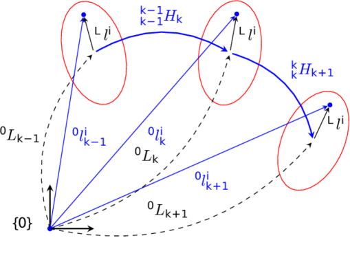
Figure 1: Representative coordinates of the rigid body in motion. The points ${}^{L}l^{i}$ are represented relative to the rigid body centre of mass $\{L\}$ at each step.

Let $\{0\}$ denote the reference coordinate frame, and $\{L\}$ a coordinate frame associated to a moving rigid body (object). We write the pose ${}^{0}L_{k}\in SE(3)$ of the rigid-body as an element of $SE(3)$ with respect to the reference frame $\{0\}$. For feature observed on an object, let ${{}^{L}}l^{i}\in{\rm I\!R}^{3}$ denote the coordinates of this point in the body-fixed frame, where ‘$i$’ is the unique index of the feature. We write ${{}^{0}}l^{i}_{k}$ for the coordinates of the same point expressed in the reference frame $\{0\}$ at time $k$. Note that for rigid bodies in motion, ${{}^{L}}l^{i}$ is constant for all the object instances, while both ${}^{0}L_{k}$ and ${{}^{0}}l^{i}_{k}$ are time varying. The point coordinates are related by the expression:

$${}^{L}{\bar{l}}^{i}=\>^{0}L_{k}^{-1}\>{}^{0}{\bar{l}}_{k}^{i}\>.$$ (1)

where ${{}^{L}}{\bar{l}}^{i}$ and ${{}^{L}}{\bar{l}}^{i}_{k}$ are the homogeneous coordinates of the points ${{}^{L}}l^{i}$ and ${{}^{0}}l^{i}_{k}$, respectively.

The relative motion of the object $L$ from time $k$ to time $k+1$ is represented by a rigid-body transformation ${}_{k}^{k}H_{k+1}\in SE(3)$ that we term the body-fixed frame pose change. Here the lower indices indicate that the transformation maps a base pose (lower left index) to a target pose lower right index, expressed in coordinates of the base frame (upper left index). The body-fixed frame pose change is the $SE(3)$ transformation:

$${}_{k}^{k}H_{k+1}=^{0}L_{k}^{-1}{{}^{0}L_{k+1}}$$ (2)

that is ‘classical’ in most robotics developments. Figure 1 shows this transformations for three consecutive object poses. In consequence, relative motion of the rigid body is given by the incremental pose transformation:

$${{}^{0}L_{k+1}}={{}^{0}L_{k}}\,{{}^{k}_{k}H_{k+1}}\>.$$ (3)

Consider a point ${}^{L}l^{i}$ in the object frame $\{L\}$. The motion of this point can be obtained by writing the expression (1) for two consecutive poses of the object at time $k$ and $k+1$ and using the relative motion of the object in (3). With that we obtain:

$${}^{0}{\bar{l}}_{k+1}^{i}=\>^{0}L_{k}\>^{k}{}_{k}H_{k+1}\>^{0}L_{k}^{-1}\>{}^{0}{\bar{l}}_{k}^{i}\>.$$ (4)

We observe that (4) relates points on the same rigid body in motion at different time step by a transformation ${}^{0}_{k}H_{k+1}=\>^{0}L_{k}\>^{k}{}_{k}H_{k+1}\>^{0}L_{k}^{-1}$, where ${}^{0}_{k}H_{k+1}\in SE(3)$. According to  [6], this equation represents a frame change of a pose transformation, and shows how the body-fixed frame pose change in (2) relates to the reference frame pose change. The point motion model in the reference frame becomes:

$${}^{0}{\bar{l}}_{k+1}^{i}=\>^{0}_{k}H_{k+1}\>^{0}{\bar{l}}_{k}^{i}\>.$$ (5)

This formulation is key to the proposed approach since it eliminates the need to estimate the actual object pose ${}^{0}L_{k}$ and allows us to work directly with points ${{}^{0}{\bar{l}}^{i}_{k}}$ in the reference frame.

Assuming the objects are moving with constant velocity is a reasonable first approximation of the motion of many moving objects such as cars, trucks, bicycles, etc, that are of interest in real world SLAM problems. The constant motion assumption is natural to pose in the body-fixed pose change:

$${{}^{k}_{k}H_{k+1}}=C={{}^{k^{\prime}}_{k^{\prime}}H_{{k^{\prime}}+1}}\in SE(3)$$ (6)

for any $k,k^{\prime}$ time indices.

A second key observation we make in this paper is that if the body-fixed frame pose change is constant then the reference frame pose change is constant too. To see this, we rescale (3) and use (6) to obtain:

$${}^{0}L_{k}=^{0}L_{k-1}\,C$$ (7)

which we replace in ${}^{0}_{k}H_{k+1}=\>^{0}L_{k}\>C\>^{0}L_{k}^{-1}$ to obtain:

$${}^{0}_{k}H_{k+1}=^{0}L_{k-1}\,C\>^{0}L_{k-1}^{-1}=\>^{0}_{k-1}H_{k}$$ (8)

It follows that the reference frame pose change:

$${{}^{0}_{k-1}H_{k}}=H={{}^{0}_{k^{\prime}}H_{{k^{\prime}}+1}}\in SE(3)$$ (9)

holds for any $k,k^{\prime}$ indices. Therefore, for a rigid-body object in motion we can use a constant reference frame pose change $H\in SE(3)$ that acts on the points on the rigid body to update their reference frame coordinates: ${}^{0}{\bar{l}}_{k+1}^{i}=H{{}^{0}{\bar{l}}^{i}_{k}}$.

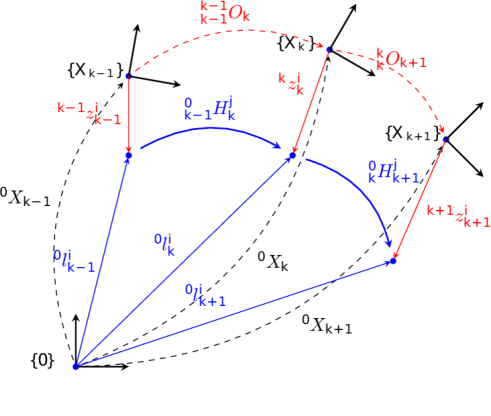
Figure 2: Representative coordinates of a system with a rigid body in motion. Blue represents state elements and red the measurements. For consistency with Figure 1, in here we show all the coordinates and relative motions in $SE(3)$, however, in the actual state vector we use the corresponding logarithm map of $SE(3)$.

III-B State representation

The SLAM with dynamic objects estimation problem is modelled using factor graphs [8], and the goal is to obtain the 3D structure of the environment (static and dynamic objects) and the robot poses that maximally satisfy a set of measurements and motion constraints. Assuming Gaussian noise, this problem becomes a non-linear least squares (NLS) optimisation over a set of variables [33]: the camera/robot poses $\textbf{x}=\{x_{0}...x_{n_{x}}\}$, with $x_{k}\in\mathfrak{se}(3)$, the tangent space of $SE(3)$ at identity, where $k\in 0...n_{x}$ and $n_{x}$ is the number of steps, and the 3D point features in the environment seen at different time steps: ${\bf l}=\{l^{1}_{0}\dots\>l^{n_{l}}_{n_{x}}\}$ where $l^{i}_{k}\in{\rm I\!R}^{3}$ and $i\in 1...n_{l}$ is the unique index of a landmark and $n_{l}$ is the total number of detected landmarks.

The set of landmarks, ${\bf l}={\bf l_{s}}\cup{\bf l_{d}}$, contains a set of static landmarks ${\bf l_{s}}$ and a set of landmarks detected on moving objects at different time steps, ${\bf l_{d}}$. The formulation in this section assumes that the static/dynamic classification and the association of the points at different time steps is done by the front-end. The same point on a moving object is represented using a different variable at each time step, i.e. $l^{i}_{k-1}$ and $l^{i}_{k}$ are the same physical point seen at time $k-1$ and $k$, respectively. In this particular problem formulation, the robot/camera poses and the positions of the 3D points are represented in the $\{0\}$ reference frame, which is omitted from their notation in this section. Nevertheless, the application of the technique is general and can easily accomodate body-fixed frame robot poses and relative points[34].

Assuming rigid body objects moving in the environment, points on the same object have similar motion. Therefore, in the proposed formulation, we integrate a new type of state variable characterising this motion. Equation (5) allows us to relate the points on moving rigid bodies at different time steps ($k$ and $k+1$) with a reference frame pose change: ${}^{0}_{k}H_{k+1}\in SE(3)$. To avoid over-parameterization, the logarithm map of an $SE(3)$ element is used as a state variable, $\{^{0}_{k}u_{k+1}^{j}\in\mathfrak{se}(3)|^{0}_{k}u_{k+1}^{j}=\log(\>^{0}_{k}H_{k+1}^{j})\}$, where $j\in 1...n_{o}$ is the object index and $n_{o}$ is the number of identified objects. The set of all variables is now ${\bf\theta}={\bf x}\cup{\bf l}\cup{\bf u}$, where ${\bf u}$ is the set of all the variables characterising the objects’ motion.

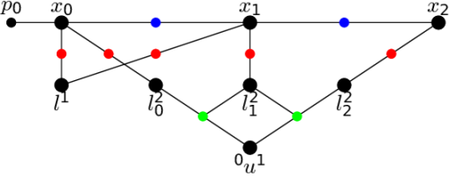
Figure 3: Factor graph representation of a problem with an SE(3) motion vertex and its edges. Superscripts represent the same landmark at different time steps. Blue factors represent odometric measurements, red factors represent point measurements in camera frames and green factors represent ‘motion factors’

III-C Measurements and object motion constraints

Two types of measurements, the odometry obtained from the robot’s proprioceptive sensors and the observations of the landmarks in the environment obtained by processing the images from an on-board camera are typically integrated into a visual SLAM application. Let $f(x_{k-1},x_{k})$ be the odometry model with $\Sigma_{v_{k}}$, odometry noise covariance matrix:

$$o_{k}=f(x_{k-1},x_{k})+v_{k}\>, v_{k}\sim\mathcal{N}(0,\Sigma_{v_{k}})\>,$$ with (10)

and $\textbf{o}=\{o_{1}...o_{m_{i}}\}$ being the set of ${m_{i}}$ odometric measurements. Similarly, let $h(x_{k},l^{i}_{k})$ be the 3D point measurement model with $\Sigma_{w_{k}}$, the measurement noise covariance matrix:

$$z_{k}^{i}=h(x_{k},l^{i}_{k})+w_{k}^{i}\>, w_{k}^{i}\sim\mathcal{N}(0,\Sigma_{w_{k}})$$ with (11)

where $\textbf{z}=\{z_{1}...z_{m_{k}}\}$, $z_{k}\in{\rm I\!R}^{3}$ is the set of all 3D point measurements at all time steps. Figure 2 shows the measurements in red.

The relative pose transformation of the points on moving rigid bodies is given in (5). Observe that the motion of any point on a specific object $j$ can be characterised by the same pose transformation ${}^{0}_{k}H_{k+1}^{j}\in SE(3)$ with ${}^{0}_{k}R_{k+1}^{j}$ the rotation component and ${}^{0}_{k}t_{k+1}^{j}$ the translation component, respectively. The factor corresponding to (5) is:

$$g(l^{i}_{k},l^{i}_{k+1},^{0}_{k}u_{k+1}^{j})={{}^{0}_{k}R_{k+1}^{j}}^{\!\top}\>{}^{0}l_{k+1}^{i}-{{}^{0}_{k}R_{k+1}^{j}}^{\!\top}\>{{}^{0}_{k}t_{k+1}^{j}}-^{0}l_{k}^{i}+q_{s_{j}}$$ (12)

with ${}^{0}_{k}R_{k+1}^{j}$ and ${{}^{0}_{k}t_{k+1}^{j}}$ obtained using the exponential map $\exp(^{0}_{k}u_{k+1}^{j})$ and $q_{s}\sim\mathcal{N}(0,\Sigma_{q})$ is the normally distributed zero-mean Gaussian noise. The factor in 12 is a ternary factor which we call the motion model of a point on a rigid body.

In this paper we analyze the effect on the solution of the SLAM problem of the assumption that the objects are moving with constant motion. Figure 3 depicts the factor graph of a small SLAM example of three robot poses, a static feature and a feature detected at three different time steps on an object with constant motion. We say that a pose change ${}^{0}_{k}H_{k+1}^{j}$ is constant for all the points on an object $j$ at every time step, hence a sole state variable ${}^{0}u^{j}$ is used for each object and the factor in (12) becomes:

$$g(l^{i}_{k},l^{i}_{k+1},^{0}u^{j})={{}^{0}R^{j}}^{\!\top}\>{}^{0}l_{k+1}^{i}-{{}^{0}R^{j}}^{\!\top}\>{{}^{0}t^{j}}-^{0}l_{k}^{i}+q_{s_{j}}$$ (13)

III-D The graph optimization

Given the measurements and motion factors introduced above, we can formulate an NLS problem to obtain the optimal solution of the SLAM with dynamic objects:

$$\boldsymbol{\theta}^{*}=\operatornamewithlimits{argmin}_{\boldsymbol{\theta}}\>\frac{1}{2}\Bigg{\{}\sum_{i=1}^{mi}\|f(x_{k-1},x_{k})-o_{k}\|_{\Sigma_{v_{k}}}^{2}+$$

$$\sum_{k=1}^{mk}\|h(x_{i},l^{i})-z_{k}\|_{\Sigma_{w_{k}}}^{2}+\sum_{i,j}^{ms}\|g(l^{i}_{k},l^{i}_{k+1},^{0}u^{j})\|_{\Sigma_{q}}^{2}\>\Bigg{\}}$$ (14)

where $mi$, $mk$ and $ms$ are the number of odometric measurements, point measurement and constant motion factors.

Iterative methods such as Gauss-Newton (GN) or Levenberg-Marquard (LM) are used to find the solution of the NLS in (14). An iterative solver starts with an initial point $\boldsymbol{\theta}^{0}$ and, at each step, computes a correction $\boldsymbol{\delta}$ towards the solution. For small $\left\|\boldsymbol{\delta}\right\|$, a Taylor series expansion leads to linear approximations in the neighborhood of $\boldsymbol{\theta}^{0}$ and a linear system $A^{\!\top}A\delta=-A^{\!\top}\bf b$ is solved at each iteration  [23, 33]. In here, $A$ gathers the derivatives of all the factors in (14) with respect to variables in $\boldsymbol{\theta}$ weighted by the square rooted covariances of each factor, and $b$ is the residual evaluated at the current linearization point. The new linearization point $\theta^{k+1}$ is obtained by applying the increment $\delta^{*}$ to the current liniarization point $\boldsymbol{\theta}^{i}$. This formulation is often used in the SLAM literature [8, 23, 25, 33].

The factor graph formulation of the SLAM problem is highly intuitive and has the advantage that it allows for efficient implementations of batch [8] [2] and incremental [24, 32, 20] NLS solvers. However the efficiency is highly reliant on the sparsity of the resulting graph. Introducing the constant motion vertex may affect the sparsity of the graph by connecting many landmark nodes to one single vertex. This can lead to inefficiency if it is not handled properly when solving the linear system. The importance of variable ordering when solving a linear system using matrix factorization has been studied in the SLAM literature [1, 32]. An appropriate permutation of the original matrix can be used, yielding small fill-in in the resulting factorization. This has significant computational advantages, since the back-substitution using a sparse triangular matrix is very efficient. Therefore, when solving the problem in (14) we insure that the motion related variables are ordered last.

(a) Experiment ‘A’

(b) Experiment ‘B’

(c) Experiment ‘C’

(d) Experiment ‘D’

(e) Experiment ‘E’

Figure 4: Different simulated robot and object trajectories. Robot trajectories are shown in blue and object trajectories in black.

IV Experimental methodology

Our SLAM system is evaluated in a number of experiments with a robot moving in dynamic environments (with moving rigid body objects). The goal is to validate the proposed methodology and evaluate the benefits of integrating them into the SLAM problem. To this end, we used several simulated datasets with ground truth, and also tested our algorithm on a real dataset.

A set of experiments were carried on simulated data obtained by emulating an advanced front-end that is capable of identifying objects, and associating detected landmarks with the different objects in the scene. In those simulations, two other types of measurements are also available; odometric measurements and point observations. Simulated data feature different robot and object trajectories of different sizes as seen in Figure 4. A second, more realistic experiment, was performed on the Virtual KITTI dataset [9]. Furthermore, real data was acquired using a Turtlebot, equipped with an RGB-D camera, odometer and IMU, which moved in an environment where two other Turtlebots are moving to emulate dynamic objects. The setup was placed in a space with a VICON motion tracking system to provide the ground truth data.

IV-A Simulated datasets

IV-A1 Experiment ‘A’

In order to test the effect of integrating the objects’ constant motion constraints, we designed an experiment where a single object is being tracked by the robot, and no static points are observed. Both robot and object are following a circular trajectory, the object having a constant motion. This experiment was repeated for $12$ different increasing lengths of the object and robot trajectories, yielding different number of ternary factors as defined in (12) ranging from $34$ to $6715$. We will refer to this set of experiments as “Experiment ‘A”’ in the remainder of this document.

IV-A2 Experiments ‘B’ $\rightarrow$ ‘E’

In order to evaluate the constant motion assumption, $4$ more experiments with multiple moving objects were generated using a simulated environment. In the first two experiments of this set (we will refer to these as “Experiments ‘B’ and ‘C’ in the remainder of this document), the objects are constrained to follow a constant motion trajectory. In the experiment ‘B’ the objects are following an elliptical trajectory as seen in Figure 4(b), while in experiment ‘C’, the objects are only translating in 3D as seen in Figure 4(c).

The constant motion assumption is violated in the following two experiments, in order to show the ability of our method to deal with non-constant motion. These experiments are referred to as“Experiments ‘D’ and ‘E’ ”, and they feature objects following a rectangular trajectory in experiment D as seen in Figure 4(d) and objects following a sine wave trajectory in experiment E. We will refer to this set of experiments as “Experiment ‘D’ $\rightarrow$ ‘E”’. These experiments were then repeated with static points in the background to show the effect of integrating object tracking into our SLAM framework, and demonstrate the improved accuracy of the estimation even when static landmarks are available.

IV-B Virtual KITTI dataset

Virtual KITTI [9] is a photo-realistic synthetic dataset designed to evaluate computer vision scene understanding algorithms. It contains $50$ high-resolution monocular videos generated from five different virtual worlds in urban settings under different imaging and weather conditions. These worlds were created using the Unity game engine and a novel real-to-virtual cloning method. The photo-realistic synthetic videos are fully annotated at the pixel level with object labels as shown in Figure 5. The depth map of each image is also available. This makes it a perfect dataset to test and evaluate the proposed technique on realistic scenarios.

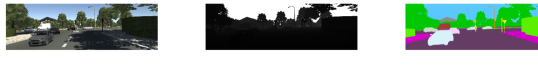
Figure 5: Examples of RGB, depth and segmentation images from the virtual Kitti dataset.

The front-end detects features in each image and obtain the 3D position relative to the camera of each point, with the aid of the corresponding depth images. The pixel-level object tracking is used to determine if these points are located on moving or static objects, and the known camera poses between frames are used to project the points to the next image in the sequence. In this manner, static and moving points are tracked between images to provide data associations between landmarks and objects as shown in Figure 6. It is possible to project points attached to moving objects to other images as the pose of all moving objects is provided by the dataset for each image. As the 3D position is tracked for all the points, along with the camera pose, the relative position of all points can be obtained for every images for which the point remains in the camera’s field of view. Upon completion of the point tracking through the chosen image set, the camera pose and relative point position are used to generate ground truth and measurement files. The noise levels added to the ground truth data in order to generate noisy measurements are as follows: $\Sigma_{v}=\mathit{diag}[0.4m,0.4m,0.4m,6^{\circ},6^{\circ},6^{\circ}]^{2}$ , $\Sigma_{w}=\mathit{diag}[0.4m,0.4m,0.4m]^{2}$ , $\Sigma_{q}=\mathit{diag}[0.05m,0.05m,0.05m]^{2}$. Our SLAM implementation can directly use these files, allowing it to be validated against the ground truth provided by the dataset. This experiment will be referred as “vKITTI” the remainder of this paper.

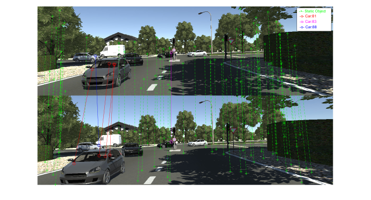
Figure 6: Feature extraction and tracking applied to the virtual kitti dataset. Static points are shown in green, and a different colour is used for points attached on each unique object.

IV-C Real dataset

The real data, was acquired using a Turtlebot equipped with an RGB-D Kinect sensor. Two other Turtlebots were covered with boxes, on which distinct colour coded landmarks were printed in order to facilitate landmark extraction, tracking and landmark/object association. Feature points landmarks on the walls and floor of the experiment space are also included in the estimation. The whole experiment is carried out in a space that is monitored by a motion capture and tracking system VICON. Three VICON markers were installed on each of the two objects and the camera robot to provide ground truth data for error analysis. This experiment will be referred to as “real experiment” in the remainder of this paper. We model the noise levels in the different sensors as follows: odometry measurement noise $\Sigma_{v}=\mathit{diag}[0.04m,0.04m,0.04m,2^{\circ},2^{\circ},2^{\circ}]^{2}$, point measurement noise $\Sigma_{w}=\mathit{diag}[0.2m,0.2m,0.2m]^{2}$, and point-SE3 motion edge noise $\Sigma_{q}=\mathit{diag}[0.05m,0.05m,0.05m]^{2}$.

IV-D Implementation details

This work was implemented into a Matlab framework which is able to integrate not only simple point measurements but also additional available information about the environment into a single SLAM framework. The object oriented design is thought to accommodate different types of information about the environment as long as there is a front-end that can provide this information and a function that can model it. The framework consists of: 1. a simulation component that can reproduce several dynamic environments; 2. a front-end that generates the data for the SLAM problem by tracking features, objects and providing point associations using simulated or real data inputs; 3. a back-end component that includes different non-linear solvers for batch and incremental processing. The estimation is implemented as a solution to an NLS problem as presented in section III and solved using Levenberg-Marquardt method. The proposed technique can be easily integrated into any of the existing SLAM back-ends  [25, 24, 20]. The code for SLAM with dynamic objects will be made publicly available upon acceptance.

V Experimental results

This section evaluates the proposed technique on the applications described in section IV. We are focused on analysing the accuracy and consistency of the proposed estimation solution and comparing it to the classical SLAM formulation which does not integrate any additional information about the motion of the 3D points in the environment.

The accuracy of the solution of the SLAM problem is evaluated by comparing the absolute trajectory translational error (ATE), the absolute trajectory rotational error (ARE), the absolute structure error (ASE), the all to all relative trajectory translational error (allRTE), the all-to-all relative trajectory rotational error (allRRE), and the all-to-all relative structure error (allRSE) calculated as in  [20].

V-A Analysis of the simulated datasets

The tests show that the proposed method helps preserving the consistency of the map and improves the estimation quality significantly. This can be seen in Figure 7 to Figure 8 and in Table I to Table III.

	Experiment A
Average errors	w/o DOM	w/ DOM	%
ATE (m)	13.834	13.58	1.82
ARE (∘)	16.21	13.75	15.1
ASE (m)	3.93	1.426	63.7
allRTE (m)	8.249	3.002	63.6
allRRE (∘)	14.103	6.859	51.3
allRSE (m)	5.408	2.015	62.7

TABLE I: Average error values for a total of 13 experiments with the motion vertex initialised as identity. ‘w/ DOM’ denotes the proposed estimation technique with dynamic object motion integrated, while ‘w/o DOM’ means that no object motion information was used in the estimation. A positive % shows improvement of ‘w/ DOM’.

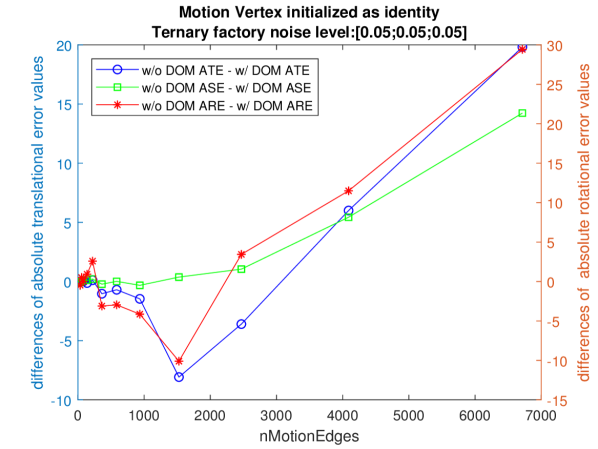
(a) Absolute error differences.

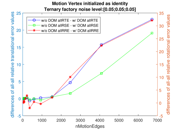
(b) Relative error differences.

Figure 7: Relative and absolute error differences computed as error metric of the SLAM solution without constant motion minus the same error metric of the SLAM solution integrating constant motion. The ‘x’ axis represents the increasing number of ternary factors.

V-A1 Experiment ‘A’

The results in Table I and Figure 7 show improvements of the estimation accuracy when the objects’ motion is integrated into the estimation. Several increasing in size SLAM problems were evaluated and the relative and absolute error differences of the pose of the robot and the location of the 3D points are reported. Positive values indicate better performance of the SLAM problem which integrate constant motion information. The general trend of the results shows that adding the motion information has a positive effect on the estimation in most of the cases. However, there are few cases where adding this constant motion vertex and the ternary factors does not benefit the solution. This is probably due to added non-linearities by the $\mathfrak{se}(3)$ type vertex which affects the convergence. Note that this experiment is showing an extreme case, where the environment has only one moving object and no static points.

	Exp.B			Exp.C
with no static points
Error	w/o DOM	w/ DOM	%	w/o DOM	w/ DOM	%
ATE (m)	0.342	0.203	40.6	0.453	0.351	22.5
ARE (∘)	6.211	3.751	39.6	6.371	4.644	27.1
ASE (m)	0.733	0.498	32.1	0.567	0.319	43.7
allRTE (m)	0.213	0.171	19.7	0.393	0.236	39.9
allRRE (∘)	5.183	3.665	29.3	5.410	5.012	7.3
allRSE (m)	1.049	0.707	32.6	0.797	0.439	44.9
with static points
ATE (m)	0.285	0.278	2.45	0.578	0.534	7.61
ARE (∘)	2.950	1.229	58.3	7.381	7.508	-1.7
ASE (m)	1.031	0.327	68.3	0.993	0.478	51.8
allRTE (m)	0.359	0.193	46.2	0.212	0.175	17.5
allRRE (∘)	3.415	1.423	58.3	4.867	3.377	30.6
allRSE (m)	1.422	0.438	69.2	1.419	0.715	49.6

TABLE II: Error values for experiments ‘B’ and ‘C’ explained in section IV-A2. ‘w/ DOM’ denotes the proposed estimation technique with dynamic object motion, while ‘w/o DOM’ means that no object motion information was used in the estimation. A positive % shows improvement of ‘w/ DOM’.

	Exp.D			Exp.E
with no static points
Error	w/o DOM	w/ DOM	%	w/o DOM	w/ DOM	%
ATE (m)	0.457	0.207	54.7	0.549	0.314	42.8
ARE (∘)	6.439	4.248	34	6.085	2.249	63
ASE (m)	1.127	0.595	47.2	0.546	0.142	73.9
allRTE (m)	0.258	0.314	-21.7	0.234	0.185	20.9
allRRE (∘)	5.719	4.180	26.9	5.655	2.674	52.7
allRSE (m)	1.505	0.811	46.1	0.73	0.202	72.3
with static points
ATE (m)	0.322	0.123	61.8	0.308	0.143	53.6
ARE (∘)	4.910	2.252	54.1	4.876	1.425	70.7
ASE (m)	1.255	0.422	66.4	0.733	0.240	67.3
allRTE (m)	0.325	0.208	36	0.320	0.178	44.4
allRRE (∘)	4.240	1.998	52.9	4.854	1.946	59.9
allRSE (m)	1.719	0.576	66.5	1.017	0.348	65.8

TABLE III: Error values for experiments ‘D’ and ‘E’ explained in section IV-A2. ‘w/ DOM’ denotes the proposed estimation technique with dynamic object motion, while ‘w/o DOM’ means that no object motion information was used in the estimation. A positive % shows improvement of ‘w/ DOM’.

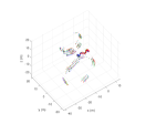
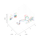
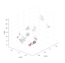
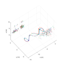
(a) Experiment ‘B’	(b) Experiment ‘C’	(c) Experiment ‘D’	(d) Experiment ‘E’

Figure 8: Solution of the SLAM with dynamic objects. Large dots represent robot trajectory and small dots represent moving points trajectories. Green - ground truth, Red - the SLAM solution without incorporating object motion information and Blue - the SLAM solution with constant motion. (best viewed in colour)

V-A2 Experiments ‘B’ $\rightarrow$ ‘E’

The upper part of the Tables II and III show the accuracy results for the Experiments ‘B’ $\rightarrow$ ‘E’ with no static points. The values indicate that adding information about the motion of the objects in the estimation process significantly improves the estimation quality and reduces the trajectory and map errors in both absolute and relative metrics. This can be seen in the positive $\%$ values in the tables. Surprisingly, the improvement persists in Experiments ‘D’ and ‘E’ where the constant motion assumption is slightly violated. The explanation for that is that the estimator compromises in estimating the constant pose transformation and satisfying the point measurements in both cases. Same noise levels were used for the ternary factors, the point measurements and the odometry across the four experiments. Qualitative evaluation of the same experiments is shown in Figure 8. Note that the ground truth (in green) and the SLAM accounting for constant motion (in blue) have similar values, while without accounting for the constant motion (in red) diverges from the ground truth.

The lower part of the Tables II and III show the accuracy results for the Experiments ‘B’ $\rightarrow$ ‘E’ where static points were also integrated into the system. We note here overall increase in accuracy due to the know effect of the static points data association on the SLAM solution.

V-A3 Experiment “vKITTI”

An experiment was run over a total of $295$ vertices, including robot poses, static and dynamic landmark positions and constant motion vertices resulting in a total $508$ edges, of which $216$ are object motion related ternary factors. The bottom part of the Table IV shows the accuracy of the SLAM solution obtained with and without constant motion information. As expected, the solution of the estimation improves when accounting for moving objects in the scene.

	Real data Exp.
Error	w/o DOM	w/ DOM	%
ATE (m)	1.112	0.981	11
ARE (∘)	28.021	27.654	1
ASE (m)	1.195	0.963	19
allRTE (m)	0.025	0.023	19
allRRE (∘)	1.681	1.533	8
allRSE (m)x$10^{-3}$	0.042	0.035	16%
	vKITTI Exp.
ATE (m)	3.060	1.439	52.9
ARE (∘)	13.270	3.970	70.0
ASE (m)	1.864	0.845	54.7
allRTE (m)	3.055	0.874	71.4
allRRE (∘)	9.289	3.361	63.8
allRSE (m)x$10^{-3}$	2.736	1.166	57.4

TABLE IV: Result values for the real dataset and vKITTI experiments. “w/ DOM” denotes the proposed estimation technique with constrained object motion, while “w/o” means that no object motion information was used in the estimation.

V-B Analysis of the real dataset

The real dataset is used to validate the algorithm on a real world scenario. However the problem size is small ($71$ vertices and $194$ edges, with the motion information integrated and only $69$ vertices and $165$ edges with no motion information added). In general, the significant improvements are mostly in the 3D points estimation, and this is because the new constant motion vertex and the ternary factors act directly on the structure points. Importantly, the value of the noise level $\Sigma_{q}$ assigned to the motion edge impacts the solution significantly. Modelling using low noise values could be too risky, as in a real scenarios the object’s motion is never constant, likewise high noise levels would result in an estimation that does not rely on the added motion information and would bring no benefit to the system.

VI Conclusion and future work

In this paper we proposed a new pose change representation for SLAM with dynamic objects and integrated it into a SLAM framework. The formulation has the advantage that no additional object pose or object geometry is required in order to account for the moving objects in SLAM. The framework works with simple SLAM front-ends capable of tracking feature points, detecting objects, and associating feature points to the objects in a sequence of images. Furthermore, we have analyzed the effect of integrating information about the objects’ motion in the environment on the accuracy and consistency of the SLAM problem. In particular, we tested the constant motion assumption. Results show good improvements in the estimation quality and consistency of the result versus the same problem with no added object motion information. Although the examples presented in this paper use the prior information that the objects have a constant motion, the proposed formulation can easily be adapted to other types of motion and in the near future work we plan to examine different solutions.

Another important issue to be analyzed in the future is the computational complexity of SLAM with object dynamic objects. It is important to note that without further reductions, the problem can become intractable in large-scale environments with many moving objects. But at the same time state reduction can be easily implemented using a windowing approach that mantains only a small set of objects points in the state rather than the points observed along the entire trajectory. A principled way to do that is to analyze how much the old observation observations contribute to the solution of the SLAM problem [24, 32, 34]. In the future, we plan to restrict the optimization problem to relevant state space, and produce scalable solutions.

Finally we plan to tackle the problems of object segmentation and data association using state of the-art deep learning techniques [10, 15, 35] to achieve a full end-to-end SLAM system.

References

- Agarwal and Olson [2012] Pratik Agarwal and Edwin Olson. Variable reordering strategies for SLAM. In IEEE/RSJ International Conference on Intelligent Robots and Systems (IROS), 2012, pages 3844–3850. IEEE, 2012.
- [2] Sameer Agarwal, Keir Mierle, and Others. Ceres solver. http://ceres-solver.org.
- Ayache and Faugeras [1989] Nicholas Ayache and Olivier D Faugeras. Maintaining representations of the environment of a mobile robot. IEEE Transactions on Robotics and Automation, 5(6):804–819, 1989.
- Bibby and Reid [2007] Charles Bibby and Ian Reid. Simultaneous Localisation and Mapping in Dynamic Environments (SLAMIDE) with reversible data association. In Proceedings of Robotics: Science and Systems, 2007.
- Cheeseman et al. [1987] P Cheeseman, R Smith, and M Self. A stochastic map for uncertain spatial relationships. In 4th International Symposium on Robotic Research, pages 467–474, 1987.
- Chirikjian et al. [2017] Gregory S. Chirikjian, Robert Mahony, Sipu Ruan, and Jochen Trumpf. Pose changes from a different point of view. In Proceedings of the ASME International Design Engineering Technical Conferences (IDETC) 2017. ASME, 2017.
- de la Puente and Rodríguez-Losada [2014] Paloma de la Puente and Diego Rodríguez-Losada. Feature based graph-SLAM in structured environments. Autonomous Robots, 37(3):243–260, 2014.
- Dellaert and Kaess [2006] Frank Dellaert and Michael Kaess. Square Root Sam: Simultaneous localization and mapping via square root information smoothing. The International Journal of Robotics Research, 25(12):1181–1203, 2006.
- Gaidon et al. [2016] A Gaidon, Q Wang, Y Cabon, and E Vig. Virtual Worlds as Proxy for Multi-Object Tracking Analysis. In CVPR, 2016.
- Girshick et al. [2018] Ross Girshick, Ilija Radosavovic, Georgia Gkioxari, Piotr Dollár, and Kaiming He. Detectron. https://github.com/facebookresearch/detectron, 2018.
- Grisetti et al. [2007] Giorgio Grisetti, Cyrill Stachniss, Slawomir Grzonka, and Wolfram Burgard. A Tree Parameterization for Efficiently Computing Maximum Likelihood Maps using Gradient Descent. In Robotics: Science and Systems, pages 27–30, 2007.
- Grisetti et al. [2010] Giorgio Grisetti, Rainer Kummerle, Cyrill Stachniss, and Wolfram Burgard. A tutorial on graph-based SLAM. IEEE Intelligent Transportation Systems Magazine, 2(4):31–43, 2010.
- Hahnel et al. [2002] Dirk Hahnel, Dirk Schulz, and Wolfram Burgard. Map building with mobile robots in populated environments. In IEEE/RSJ International Conference on Intelligent Robots and Systems, 2002., volume 1, pages 496–501. IEEE, 2002.
- Hahnel et al. [2003] Dirk Hahnel, Rudolph Triebel, Wolfram Burgard, and Sebastian Thrun. Map building with mobile robots in dynamic environments. In IEEE International Conference on Robotics and Automation, 2003. Proceedings. ICRA’03, volume 2, pages 1557–1563. IEEE, 2003.
- He et al. [2017] Kaiming He, Georgia Gkioxari, Piotr Dollár, and Ross Girshick. Mask R-CNN. In IEEE International Conference on Computer Vision (ICCV), 2017, pages 2980–2988. IEEE, 2017.
- Henein et al. [2017] Mina Henein, Montiel Abello, Viorela Ila, , and Robert Mahony. Exploring The Effect of Meta-Structural Information on the Global Consistency of SLAM. In IEEE/RSJ International Conference on Intelligent Robots and Systems 2017. The Australian National University, 2017.
- Hoiem et al. [2008] Derek Hoiem, Alexei A Efros, and Martial Hebert. Putting objects in perspective. International Journal of Computer Vision, 80(1):3–15, 2008.
- Hsiao et al. [2017] Ming Hsiao, Eric Westman, Guofeng Zhang, and Michael Kaess. Keyframe-based dense planar SLAM. In IEEE International Conference on Robotics and Automation (ICRA), 2017, pages 5110–5117. IEEE, 2017.
- Ila et al. [2015] Viorela Ila, Lukáš Polok, Marek Šolony, Pavel Smrž, and Pavel Zemčík. Fast covariance recovery in incremental nonlinear least square solvers. pages 4636–4643, May 2015. doi: 10.1109/ICRA.2015.7139841.
- Ila et al. [2017] Viorela Ila, Lukáš Polok, Marek Šolony, and Pavel Svoboda. SLAM++-A highly efficient and temporally scalable incremental SLAM framework. International Journal of Robotics Research, Online First(0):1–21, 2017. doi: 10.1177/0278364917691110.
- Julier and Uhlmann [2001] Simon J Julier and Jeffrey K Uhlmann. A counter example to the theory of simultaneous localization and map building. In IEEE International Conference on Robotics and Automation (ICRA), Proceedings 2001, volume 4, pages 4238–4243. IEEE, 2001.
- Kaess [2015] Michael Kaess. Simultaneous Localization and Mapping with Infinite Planes. In IEEE International Conference on Robotics and Automation (ICRA), 2015, pages 4605–4611. IEEE, 2015.
- Kaess et al. [2008] Michael Kaess, Ananth Ranganathan, and Frank Dellaert. iSAM: Incremental Smoothing and Mapping. IEEE Transactions on Robotics, 24(6):1365–1378, 2008.
- Kaess et al. [2011] Michael Kaess, Hordur Johannsson, Richard Roberts, Viorela Ila, John J Leonard, and Frank Dellaert. iSAM2: Incremental smoothing and mapping using the bayes tree. The International Journal of Robotics Research, page 0278364911430419, 2011.
- Kümmerle et al. [2011] Rainer Kümmerle, Giorgio Grisetti, Hauke Strasdat, Kurt Konolige, and Wolfram Burgard. g2o: A general framework for graph optimization. In IEEE International Conference on Robotics and Automation (ICRA), 2011, pages 3607–3613. IEEE, 2011.
- Leibe et al. [2007] Bastian Leibe, Nico Cornelis, Kurt Cornelis, and Luc Van Gool. Dynamic 3D scene analysis from a moving vehicle. In Computer Vision and Pattern Recognition, 2007. CVPR’07. IEEE Conference on, pages 1–8. IEEE, 2007.
- Leonard et al. [1992] John J Leonard, Hugh F Durrant-Whyte, and Ingemar J Cox. Dynamic map building for an autonomous mobile robot. The International Journal of Robotics Research, 11(4):286–298, 1992.
- Lu and Milios [1997] Feng Lu and Evangelos Milios. Globally consistent range scan alignment for environment mapping. Autonomous robots, 4(4):333–349, 1997.
- Miller and Campbell [2007] Isaac Miller and Mark Campbell. Rao-blackwellized particle filtering for mapping dynamic environments. In IEEE International Conference on Robotics and Automation, 2007, pages 3862–3869. IEEE, 2007.
- Montesano et al. [2008] Luis Montesano, Javier Minguez, and Luis Montano. Modeling dynamic scenarios for local sensor-based motion planning. Autonomous Robots, 25(3):231–251, 2008.
- Mu et al. [2016] Beipeng Mu, Shih-Yuan Liu, Liam Paull, John Leonard, and Jonathan P How. SLAM with objects using a nonparametric pose graph. In IEEE/RSJ International Conference on Intelligent Robots and Systems (IROS), 2016, pages 4602–4609. IEEE, 2016.
- Polok et al. [2013a] Lukas Polok, Viorela Ila, Marek Solony, Pavel Smrz, and Pavel Zemcik. Incremental Block Cholesky Factorization for Nonlinear Least Squares in Robotics. In Proceedings of Robotics: Science and Systems, Berlin, Germany, June 2013a. doi: 10.15607/RSS.2013.IX.042.
- Polok et al. [2013b] Lukas Polok, Marek Solony, Viorela Ila, Pavel Smrz, and Pavel Zemcik. Efficient implementation for block matrix operations for nonlinear least squares problems in robotic applications. In IEEE International Conference on Robotics and Automation (ICRA), 2013, pages 2263–2269. IEEE, 2013b.
- Polok et al. [2015] Lukáš Polok, Vincent Lui, Viorela Ila, Thomas Drummond, and Robert Mahony. The Effect of Different Parameterisations in Incremental Structure from Motion. In Australasian Conference on Robotics and Automation (Robert Mahony 02 December 2015 to 04 December 2015), pages 1–9. The Australian National University, 2015.
- Redmon et al. [2016] Joseph Redmon, Santosh Divvala, Ross Girshick, and Ali Farhadi. You only look once: Unified, real-time object detection. In Proceedings of the IEEE conference on computer vision and pattern recognition, pages 779–788, 2016.
- Rogers et al. [2010] John G Rogers, Alexander JB Trevor, Carlos Nieto-Granda, and Henrik I Christensen. SLAM with expectation maximization for moveable object tracking. In IEEE/RSJ International Conference on Intelligent Robots and Systems (IROS), 2010, pages 2077–2082. IEEE, 2010.
- Salas-Moreno et al. [2013] Renato F Salas-Moreno, Richard A Newcombe, Hauke Strasdat, Paul HJ Kelly, and Andrew J Davison. SLAM++: Simultaneous Localisation and Mapping at the Level of Objects. In IEEE Conference on Computer Vision and Pattern Recognition (CVPR), 2013, pages 1352–1359. IEEE, 2013.
- Walcott-Bryant et al. [2012] Aisha Walcott-Bryant, Michael Kaess, Hordur Johannsson, and John J Leonard. Dynamic pose graph SLAM: Long-term mapping in low dynamic environments. In 2012 IEEE/RSJ International Conference on Intelligent Robots and Systems, pages 1871–1878. IEEE, 2012.
- Wang et al. [2003] Chieh-Chih Wang, Charles Thorpe, and Sebastian Thrun. Online simultaneous localization and mapping with detection and tracking of moving objects: Theory and results from a ground vehicle in crowded urban areas. In IEEE International Conference on Robotics and Automation, 2003. Proceedings. ICRA’03, volume 1, pages 842–849. IEEE, 2003.
- Wang et al. [2007] Chieh-Chih Wang, Charles Thorpe, Sebastian Thrun, Martial Hebert, and Hugh Durrant-Whyte. Simultaneous localization, mapping and moving object tracking. The International Journal of Robotics Research, 26(9):889–916, 2007.
- Wolf and Sukhatme [2004] Denis Wolf and Gaurav S Sukhatme. Online simultaneous localization and mapping in dynamic environments. In IEEE International Conference on Robotics and Automation, 2004. Proceedings. ICRA’04, volume 2, pages 1301–1307. IEEE, 2004.
- Wolf and Sukhatme [2005] Denis F Wolf and Gaurav S Sukhatme. Mobile robot simultaneous localization and mapping in dynamic environments. Autonomous Robots, 19(1):53–65, 2005.
- Xiang et al. [2015] Yu Xiang, Alexandre Alahi, and Silvio Savarese. Learning to track: Online multi-object tracking by decision making. In IEEE international conference on computer vision (ICCV),2015, number EPFL-CONF-230283, pages 4705–4713. IEEE, 2015.
- Zhang et al. [2008] Li Zhang, Yuan Li, and Ramakant Nevatia. Global data association for multi-object tracking using network flows. In IEEE Conference on Computer Vision and Pattern Recognition (CVPR), 2008, pages 1–8. IEEE, 2008.
- Zhao et al. [2008] Huijing Zhao, Masaki Chiba, Ryosuke Shibasaki, Xiaowei Shao, Jinshi Cui, and Hongbin Zha. SLAM in a dynamic large outdoor environment using a laser scanner. In IEEE International Conference on Robotics and Automation, 2008. ICRA 2008., pages 1455–1462. IEEE, 2008.