Deep Learning of Geometric Constellation Shaping including Fiber Nonlinearities

1 Introduction

Optical transmission systems enabled modern data traffic applications, yet the future traffic growth is outpacing the achievable rates provided by such systems ¹. Systems with high spectral efficiency are in demand, but limited by available signal-to-noise ratio (SNR). For the additive white Gaussian noise (AWGN) channel, constellation shaping, either geometric or probabilistic, provide up to 1.53 dB gain in SNR ². Both shaping methods have been applied in fiber optics but most often optimized under an AWGN channel assumption ^{2, 3}. For the fiber optic channel, an optimal constellation is jointly robust to transmitter imperfections, amplification noise as well as signal dependent nonlinear effects ⁴. Especially, the modulation dependent nonlinear effects pose an intricate problem, since they are conditioned by the moment of the optimized constellation itself ⁵. Constellation optimization for the nonlinear channel is thus non-trivial. Machine learning is established for learning high dimensional relationships while taking various factors and constraints into account ⁶. O’Shea et al. ⁷ have shown the potential of learning codes by embedding a channel within an unsupervised machine learning algorithm, the auto-encoder ⁸. Similar, we propose, to embed fiber channel models within an auto-encoder ⁹ and learn geometric constellation shapes robust to the channel impairments, see Fig. 1. Thus, this method combines a channel model, the Gaussian noise (GN)-model ¹⁰ or the nonlinear interference noise (NLIN)-model ⁵, with gradient based optimization from machine learning. Together, a computational graph is composed with all the information inherit in the channel model and enough flexibility to optimize for a geometric constellation shape. Trained on the GN-model, the learned constellation is optimized for an AWGN channel with an effective SNR governed by the launch power, thus nonlinear effects are not being mitigated. Trained on the NLIN-model the learned constellation mitigates nonlinear effects by optimizing its moment.

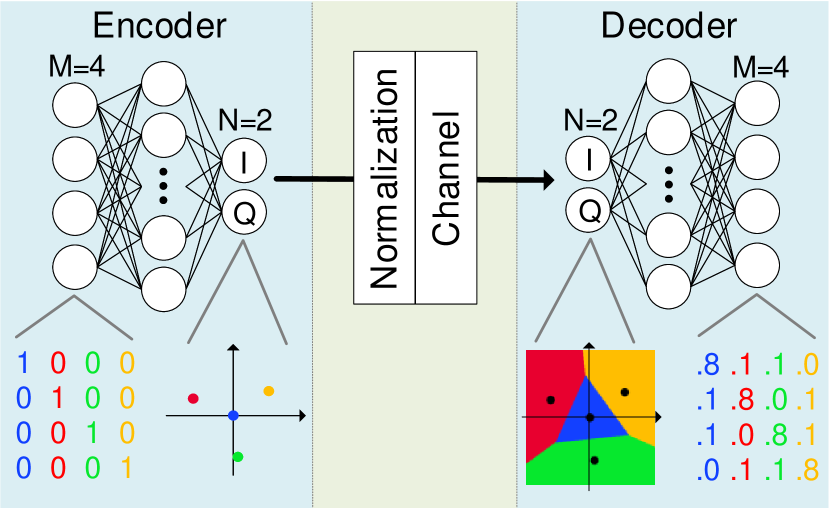
Figure 1: Trainable auto-encoder model.

The performance in mutual information (MI) of the learned constellations is estimated with the NLIN-model and simulations using the split-step Fourier (SSF) method. Up to 0.13 bit/4D of gains are reported with respect to iterative polar modulation (IPM)-based geometrically shaped constellations ³.

2 Channel Model and Auto-Encoder

The unsupervised learning method embeds a channel model within an auto-encoder, as shown in Fig. 1. The fiber channel is modeled by the NLIN-model, where the channel impairments only depend on the amplified spontaneous emission (ASE) noise, the average channel power $P$, and the 4th and 6th order moment ($\kappa$ and $\kappa_{3}$) of the constellation. The discrete NLIN-model is described as follows ⁵:

$$\begin{split}y&=c(x,P^{3},\kappa,\kappa_{3})\\ &=x+n_{\text{ASE}}+n_{\text{NLIN}},\end{split}$$ (1)

where $y$ and $x$ are the received and transmitted symbols, $c(\cdot)$ the channel model, and $n_{\text{ASE}}\sim N(0,\sigma^{2}_{\text{ASE}})$ and $n_{\text{NLIN}}\sim N(0,\sigma^{2}_{\text{NLIN}}(P^{3},\kappa,\kappa_{3}))$ are Gaussian noise samples with variance $\sigma^{2}_{\text{ASE}}$ and $\sigma^{2}_{\text{NLIN}}$, respectively. For the GN-model the dependence on $\kappa$ and $\kappa_{3}$ is dropped, removing the modulation dependent nonlinear effect. Wrapping the channel model with encoder and decoder, both as neural networks (NN), constructs the trainable auto-encoder model. NNs operate with vectors of real numbers, thus the symbols $x$ and $y$ are transcribed into vectors of their real and imaginary part. The auto-encoder model is defined as follows:

$$\begin{split}\vec{x}&=f(\vec{s}),\\ \vec{y}&=c(\vec{x},P^{3},\kappa,\kappa_{3}),\\ \vec{r}&=g(\vec{y}),\\ L&(\vec{s},\vec{r}=g(c(f(\vec{s})))),\end{split}$$ (2)

where $f(\cdot)$ is the encoder NN, $g(\cdot)$ the decoder NN. The goal is to reproduce the input $\vec{s}$ at the output $\vec{r}$ through a latent variable $\vec{x}$ (and its impaired version $\vec{y}$). This is achieved by minimizing a loss function $L(\cdot)$ such that $\vec{s}\approx\vec{r}$. An $N$ dimensional constellation is obtained with $\vec{x}$ chosen as $N$ dimensional vector. A constellation of order $M$ is enforced by training the auto-encoder with one-hot encoded vectors $\vec{s}\in S=\{\vec{e}_{i}\leavevmode\nobreak\ |\leavevmode\nobreak\ i=1..M\}$, where $\vec{e}_{i}$ is the all zero vector except at row $i$, and which implies $|S|=M$. The model is trained identical to a traditional auto-encoder. Multiple instances of $\vec{s}$ are uniformly sampled from $S$ and propagated through the auto-encoder model. The error obtained through the loss function is then backpropagated to optimize the NN weights. The optimization is gradient based and step wise, which means, the free parameters of the encoder and decoder are optimized iteratively towards a state where the input is reproduced at the output. For further illustration $N$=2 and $M$=4 are chosen, see Fig. 1. Thus, an instance of $\vec{x}$ represents a point as in-phase and quadrature (IQ) components and $\vec{s}$ is uniformly sampled from one-hot encoded vectors of length 4. In that sense, $\vec{s}$ represents the source of the system, but does not determine the actual constellation. The encoder learns a bijective projection from $\vec{s}$ to $\vec{x}$, thus for every element in $S$, one point in the IQ plane is obtained. All points together resembe a constellation of order 4. After the channel, the decoder classifies the impaired symbols $\vec{y}$ back to estimates of one-hot encoded vectors $\vec{r}$. The decoder has learned decision boundaries in between the impaired symbols, at the same time as the encoder was forced to produce a distinguishable set of symbols given the channel impairment.

3 Numerical Simulation

The auto-encoder method described above is used to find the optimal constellation for both, a channel governed by the NLIN-model and the GN-model. The auto-encoder optimizes the constellation but thereafter only the learned constellation is used, meaning an NN is neither required at the deployed transmitter nor receiver. The auto-encoder model is trained for each tested transmission distance and launch power. The performance of the learned constellations is validated using both the NLIN-model and SSF simulations. The SSF method simulates a dual polarization WDM system of 5 channels with 50 GHz channel spacing, each channel is root raised cosine shaped with 0.05 roll-off factor and 32 GHz bandwidth. The propagation is governed by 0.2 dB/km attenuation, dispersion coefficient 16.46 ps/(nm km), nonlinear coefficient 1.3 (W km)^-1 , and 20 spans of 100 km length. The power level is swept from -5 dBm to 5 dBm. The NLIN-model, which assumes Nyquist shaped pulses, is used for all other performance estimations with 5 to 55 number of spans. The results are compared to the performance of $M$-QAM constellations and IPM type geometrically shaped constellations ³.

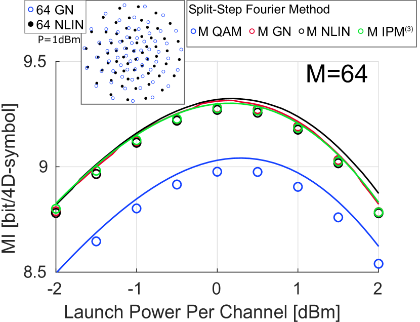
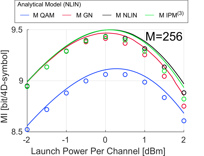
Figure 2: Performance in MI with respect to launch power after 2000 km transmission (20 spans) for $M$=64 (left) and $M$=256 (right). Plots denoted as ”$M$ GN” and ”$M$ NLIN” indicate that the constellation was learned using the GN-model and NLIN-model, respectively. Lines depict performance evaluations using the NLIN-model and markers using the SSF method. (top-left) Learned $M$=64 constellation for 2000 km transmission and 1 dBm launch power.

4 Results and Discussion

The simulation results for a 2000 km transmission (20 spans) are shown in Fig. 2. The auto-encoder constellations obtain improved performance in MI compared to standard QAM constellations. Further, the optimal launch power for constellations trained on the NLIN-model is shifted towards higher powers compared to the GN-model and IPM-based constellations. In Fig. 3, at higher power the gain with respect to standard QAM constellations is larger for the NLIN-model obtained constellations, and in Fig. 4 (top), the constellations learned with the NLIN-model have a negative slope in moment. This shows that the auto-encoder wrapping the NLIN-model, learns constellations causing less nonlinearities by reducing the moments.

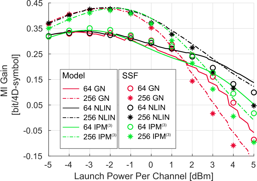
Figure 3: Gain compared to the standard $M$-QAM constellations with respect to launch power after 2000 km transmission (20 spans).

At optimal launch power and transmission distances of 2500 km to 5500 km, the difference between NLIN-model, GN-model and IPM-based constellations are marginal, Fig. 4 (bottom). However, at lower transmission distance the auto-encoder learned constellations outperform the IPM-based constellations by up to 0.13 bit/4D, since with less accumulated dispersion the signal dependent nonlinearities prevail ⁵. The marginal improvement over state of the art constellations at longer transmission distance suggests that temporal effects must be taken into account for larger gains.

5 Conclusions

An optimization method for geometric constellation shapes is proposed, by the means of an unsupervised learning method known as auto-encoder. With a channel model including modulation dependent nonlinear effects, the deep learning algorithm yields a constellation mitigating these, with gains up to 0.13 bit/4D. The method is used as is without any further analytic derivations necessary, since the machine learning optimization method is agnostic to the embedded channel model.

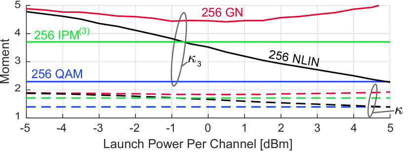
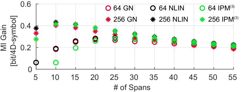
Figure 4: (top) 4th and 6th order moment ($\kappa$ and $\kappa_{3}$) of constellations with $M$=256 with respect to launch power optimized for 2000 km transmission distance.
(bottom) Gain compared to the standard $M$-QAM constellations at the respective optimal launch power with respect to number of spans.

6 Acknowledgements

We thank Dr. Tobias Fehenberger for discussions on the used channel models. This work was financially supported by Keysight Technologies (Germany, Böblingen).

References

- 1 R.-J. Essiambre et al. ”Capacity limits of optical fiber networks.” JLT 28.4 (2010): 662-701.
- 2 T. Fehenberger et al. ”On probabilistic shaping of quadrature amplitude modulation for the nonlinear fiber channel.” JLT 34.21 (2016): 5063-5073.
- 3 I. B. Djordjevic et al. ”Coded polarization-multiplexed iterative polar modulation (PM-IPM) for beyond 400 Gb/s serial optical transmission.” OFC, paper OMK2, (2010).
- 4 M. P. Yankov et al. ”Constellation shaping for WDM systems using 256QAM/1024QAM with probabilistic optimization.” JLT 34.22 (2016): 5146-5156.
- 5 R. Dar et al. ”Properties of nonlinear noise in long, dispersion-uncompensated fiber links.” Opt. Exp. 21.22 (2013): 25685-25699.
- 6 D. Zibar et al. ”Machine learning under the spotlight.” Nature Photonics 11.12 (2017): 749.
- 7 T. O’Shea and J. Hoydis. ”An introduction to deep learning for the physical layer.” TCCN 3.4 (2017): 563-575.
- 8 I. Goodfellow et al. ”Deep learning.” Cambridge: MIT press, (2016).
- 9 B. Karanov et al. ”End-to-end deep learning of optical fiber communications.” arXiv:1804.04097 (2018).
- 10 P. Poggiolini et al. ”The GN model of non-linear propagation in uncompensated coherent optical systems.” JLT 30.24 (2012): 3857-3879.