Emergence and spontaneous breaking of approximate $\mathrm{O}(4)$ symmetry
at a weakly first-order deconfined phase transition

Abstract

We investigate approximate emergent nonabelian symmetry in a class of weakly first order ‘deconfined’ phase transitions using Monte Carlo simulations and a renormalization group analysis. We study a transition in a 3D classical loop model that is analogous to a deconfined 2+1D quantum phase transition in a magnet with reduced lattice symmetry. The transition is between the Néel phase and a twofold degenerate valence bond solid (lattice-symmetry-breaking) phase. The combined order parameter at the transition is effectively a four-component superspin. It has been argued that in some weakly first order ‘pseudocritical’ deconfined phase transitions, the renormalization group flow can take the system very close to the ordered fixed point of the symmetric $O(N)$ sigma model, where $N$ is the total number of ‘soft’ order parameter components, despite the fact that $O(N)$ is not a microscopic symmetry. This yields a first order transition with unconventional phenomenology. We argue that this occurs in the present model, with $N=4$. This means that there is a regime of lengthscales in which the transition resembles a ‘spin-flop’ transition in the ordered $O(4)$ sigma model. We give numerical evidence for (i) the first order nature of the transition, (ii) the emergence of $O(4)$ symmetry to an accurate approximation, and (iii) the existence of a regime in which the emergent $O(4)$ is ‘spontaneously broken’, with distinctive features in the order parameter probability distribution. These results may be relevant for other models studied in the literature, including 2+1D QED with two flavours, the ‘easy-plane’ deconfined critical point, and the Néel–VBS transition on the rectangular lattice.

I Introduction

The phenomenology of deconfined criticality deccp ; deccplong in models with small ‘$N$’ — for example spin-1/2 magnets with various symmetries in 2+1D SandvikJQ ; melkokaulfan ; lousandvikkawashima ; Banerjeeetal ; Sandviklogs ; Kawashimadeconfinedcriticality ; Jiangetal ; deconfinedcriticalityflowJQ ; kukloveasyplane ; kuklovetalDCPSU(2) ; kaulsandviklargen ; sandvik2parameter ; kauleasyplane1 ; qin2017duality ; zhang2018continuous , and related classical models DCPscalingviolations ; emergentso5 ; sreejith2018emergent ; powellmonopole — has turned out to be more interesting and more subtle than could have been guessed from simple large $N$ approximations. Many phenomena have been invoked in order to explain perplexing numerical results: we are gradually elucidating which are only mirages, and which are the crucial features of the problem. Here we demonstrate a remarkable weakly first-order ‘deconfined’ phase transition, with unusual phenomenology, in a model with two competing order parameters. This phase transition combines the ingredient of emergent symmetry with that of ‘quasiuniversality’ DCPscalingviolations ; wang2017deconfined at weakly first order deconfined transitions.

Emergent nonabelian symmetries, which unite distinct order parameters, are a key concept for understanding deconfined criticality in small ‘$N$’ models tsmpaf06 ; tanakahu ; emergentso5 ; wang2017deconfined . At the Néel to valence-bond-solid (Néel–VBS) transition in square lattice spin-1/2 magnets, with full spin rotation symmetry, five order parameter components become ‘soft’ at the transition. These are the three components of the Néel vector $\bm{\mathbf{N}}$ and the two components of the VBS order parameter $\bm{\mathbf{\phi}}$. Numerics show a very accurate $SO(5)$ symmetry uniting these five components at the transition emergentso5 ; sreejith2018emergent ; SandvikSpectrum . We may write them as a superspin,

$${\bf n}=(N_{x},N_{y},N_{z},\phi_{x},\phi_{y}).$$ (1)

At currently accessible system sizes, the $SO(5)$ symmetry for $\bm{\mathbf{n}}$ looks like exact symmetry of the infra-red theory, which becomes increasingly accurate at longer lengthscales. At asymptotically long lengthscales it may well only be an approximate symmetry (see wang2017deconfined ; sreejith2018emergent ; PolandReview for discussions), but it seems to be a robust feature of models described by the noncompact $\mathrm{CP}^{1}$ field theory ($\mathrm{NCCP}^{1}$ motrunichvishwanath1 ) originally proposed for the Neel-VBS transition deccp . For example, $SO(5)$ also emerges sreejith2018emergent in a classical dimer model that has very different microscopic symmetries to the Néel–VBS models PowellChalkerPRL ; CharrierAletPujol ; Chenetal ; PowellChalkerPRB . Emergent $SO(5)$ is equivalent to an infra-red self-duality of the $\mathrm{NCCP}^{1}$ field theory, and it also opens up the possibility of relationships with other field theories, including two-flavour quantum chromodynamics wang2017deconfined . A variant of the latter has recently been proposed to describe a confinement transition with emergent $SO(5)$ gazit2018confinement .

A different class of putative ‘deconfined’ phase transitions are those involving only four soft order parameter components. The best-studied example is the ‘easy-plane’ Néel–VBS transition, with two Néel and two VBS components kukloveasyplane ; kragseteasyplane ; kauleasyplane1 ; kauleasyplane2 ; qin2017duality ; zhang2018continuous ; motrunichvishwanath1 ; motrunichvishwanath2

$${\bf n}=(N_{x},N_{y},\phi_{x},\phi_{y}).$$ (2)

It was suggested that this transition, if continuous, may have emergent $O(4)$ symmetry wang2017deconfined ; qin2017duality . There are models where the transition is clearly first order kukloveasyplane ; kragseteasyplane ; kauleasyplane1 ; kauleasyplane2 ; Chenetal (including a self-dual motrunichvishwanath1 lattice model geraedtsmotrunich1 ; geraedtsmotrunich2 ), but it has recently been claimed that the transition is continuous in other models qin2017duality ; zhang2018continuous . It was also pointed out recently metlitski2017intrinsic ; sato2017dirac that the same $O(4)$–invariant long-distance theory may well apply to another set of transitions: these have full ${SO}(3)$ spin rotation symmetry, but only a one-component VBS order parameter tsmpaf06 :

$${\bf n}=(N_{x},N_{y},N_{z},\varphi).$$ (3)

In this last set of examples there is, loosely speaking, a semi-microscopic $SO(3)\times\mathbb{Z}_{2}$ symmetry, where the $\mathbb{Z}_{2}$ really refers to lattice symmetries (e.g. translation) that change the sign of the VBS order parameter $\varphi$.

One member of this class is the Néel–VBS transition on a square lattice with rectangular anisotropy, which suppresses one of the two possible directions for the columnar VBS order parameter metlitski2017intrinsic ; tsmpaf06 . Another is a Néel to (twofold degenerate) VBS transition that has been studied in a fermionic model on the honeycomb lattice: numerics support emergent $O(4)$ symmetry here sato2017dirac . A third example is a transition metlitski2017intrinsic for spin-1s on the isotropic square lattice, between the Néel phase and a VBS phase WangNematicity2015 ; KomargodskiWalls2018 with two degenerate ground states.

The 3D classical transition we study below is analogous to a 2+1D Néel–VBS transition for spin-1/2s on a square lattice with reduced lattice symmetry, and also has a four-component order parameter of the form in Eq. 3, with $SO(3)\times{\mathbb{Z}_{2}}$ symmetry.

We can think of the four-component cases (2) and (3) as descending from the five-component case under deformations that disfavour one of the components of (1). It is worth noting that the relation between these deformations is highly non-obvious in the usual $\mathrm{NCCP}^{1}$ language. Easy-plane anisotropy and, say, rectangular anisotropy metlitski2017intrinsic correspond to deformations of very different types that reduce the symmetry of the $\mathrm{NCCP}^{1}$ model in different ways (easy plane anisotropy yields a quartic potential for the spinon field, while rectangular anisotropy gives a fugacity for strength-two Dirac monopoles). However if $O(4)$ symmetry emerges there is the possibility that these various models converge under RG flow. Even more strikingly, the easy-plane model has been conjectured to be dual to two-flavour quantum electrodynamics ($N_{f}=2$ QED) karchtong ; wang2017deconfined , and this theory may also acquire $O(4)$ in the infrared. A conjectured self-duality of $N_{f}=2$ QED qeddual ; karchtong ; seiberg2 ; JianEmergent2017 would imply $O(4)$ in that theory (which may also be argued for heuristically by a mapping to the $O(4)$ sigma model at $\theta=\pi$ tsmpaf06 , and which has some support from simulations KarthikFlavor2017 ).

A second useful concept is that of pseudocriticality. This is a regime of ‘slow’ renormalization group (RG) flow, associated with a more or less well-defined line in coupling constant space that attracts nearby flow lines, leading to ‘quasiuniversal’ behaviour that is only weakly dependent on the bare parameters wang2017deconfined . This phenomenon can be made precise in various field theories with a parameter that does not flow under the RG, and was proposed as an explanation for various puzzling phenomena at deconfined phase transitions in DCPscalingviolations ; wang2017deconfined . A classic example of this phenomenon is the Potts model, where as the number of states $Q$ is increased the continuous transition gives way to a first-order one at a universal critical value baxterpotts ; nienhuispotts ; nauenbergscalapino ; cardynauenbergscalapino ; IinoDetecting2018 . This is due to the annihilation of a critical and a tricritical fixed point. (Fixed point annihilation has also been discussed in QCD and QED, among other models Gies ; kaplan ; braun2014phase ; GiombiConformal2016 ; HerbutChiral2016 ; GukovRG2017 ; PhaseTransitionsCPNSigmaModel .) For $Q$ slightly larger than the critical value, there is a first order transition with a parametrically large correlation length and quasiuniversal properties that depend only parametrically weakly wang2017deconfined on the bare couplings. (See IinoDetecting2018 for a recent numerical study of the Potts case.)

In models that show a pseudocritical regime, the simplest possibility is that at the very longest lengthscales the RG flow is to a discontinuity fixed point, i.e. a first order transition. However things can be more interesting if an (approximate) emergent symmetry is established during the quasiuniversal RG flow associated with pseudocriticality, i.e. if the attractive flow line has the higher symmetry wang2017deconfined . In this case the emergent symmetry persists even into the coexistence regime — i.e. the regime of lengthscales where the order parameters no longer appear to be scaling to zero with system size (as at a critical point) but have instead saturated to a finite value. This gives an unconventional first-order transition which resembles a spin-flop transition in an ordered sigma model with the higher symmetry (i.e., a transition driven by changing the sign of an anisotropy in the sigma model). We review this RG picture below.

It is plausible that the above scenario is what ultimately happens in the models that show an emergent $SO(5)$ symmetry. But if so, the lengthscale required to see it seems to be inaccessible at present: we can access the ‘pseudocritical’ regime but not the ‘spin flop’ regime at larger scales. (It is also conceivable that the ultimate fate of the models with $SO(5)$ symmetry is something else, though this is constrained by conformal bootstrap SimmonsDuffinSO(5) ; Nakayama ; PolandReview .)

By contrast, we show here that the phenomenon of a weakly first order transition with emergent approximate $O(4)$ symmetry can be seen in models for deconfined criticality with four order parameter components, or rather in at least one such model. In the model we study the lengthscale associated with the first order transition is long enough to allow $O(4)$ to emerge with good accuracy (we demonstrate this directly using the order parameter distribution) and short enough that we can convincingly demonstrate that the transition is first-order.

The resulting first-order transition has an interesting phenomenology, because the two competing phases, which coexist at the critical coupling, are related by an effective continuous symmetry in the appropriate range of lengthscales. This has characteristic signatures in the probability distribution of the order parameters, which takes a simple universal form, and of quantities like the energy, which do not have the double peaked shape familiar in conventional first order transitions. The model we study is a classical 3D loop model DCPscalingviolations that is closely related to a deconfined critical point for 2+1D square lattice magnets, but with reduced lattice symmetry (the loop model can be viewed as a deformation of the partition function of a quantum magnet to impose isotropy in the three ‘spacetime’ dimensions, making the model more convenient for simulations). We argue that this model shows the basic features of the RG scenario outlined above.

Work on field theoretic dualities has recently revealed unexpected connections between 2+1D field theories, and as a result the present results are relevant to a variety of other models. Various examples of deconfined criticality with four order-parameter components have been discussed in the literature, and as mentioned above the easy-plane transition has been argued to be dual to 2+1D quantum electrodynamics with $N_{f}=2$. It would be worth looking for the phenomena we discuss in those models. (The status of duality webs relating different theories, in cases where the emergent symmetry implied by the dualities is approximate rather than exact, is discussed in wang2017deconfined .) Recent numerics has however argued for a continuous easy-plane transition rather than a weakly first-order one qin2017duality ; zhang2018continuous (see kauleasyplane2 ; JianEmergent2017 for discussions of relations between different easy-plane models), and for scale invariance in $N_{f}=2$ QED qedcft . In the light of the relationships expected between the various field theories this difference with what we find here is surprising and would be worth examining further.

II RG picture

Before describing a particular model, in this section we review the scenario of wang2017deconfined for a weakly first order deconfined phase transition with approximate emergent symmetry. For concreteness, we focus on the scenario with a four-component order parameter which will be relevant to us below. For a simplified picture, it is useful to think of the nonlinear sigma model as the effective field theory for this order parameter tsmpaf06 . This theory is not precisely defined, since the sigma model is a nonrenormalizable effective field theory whose definition is regularization dependent, but this will not matter for the following qualitative discussion of the RG flows (see wang2017deconfined for a more careful discussion).

The sigma model for the four-component field ${\bf n}$, with ${\bf n^{2}}=1$, is

$$\mathcal{L}=\frac{1}{2g}(\partial{\bf n})^{2}+\frac{i\pi\epsilon_{abcd}}{\text{Area}(S^{3})}n_{a}\partial_{x_{1}}n_{b}\partial_{x_{2}}n_{c}\partial_{x_{3}}n_{d}+\ldots$$ (4)

The second term is the topological $\Theta$ term whose presence was argued for in tsmpaf06 (see also tanakahu for a related discussion of the 5-component case). The ‘$\ldots$’ include perturbations that reduce the symmetry to the microscopic symmetry of the lattice model of interest.

These perturbations can be classified into representations of $O(4)$ symmetry. We assume that the ones which are important for us in the pseudocritical regime (described below) — i.e. the most relevant allowed perturbations — are two- and four-index symmetric traceless $O(4)$ tensors $X^{(2)}_{ab}$ and $X^{(4)}_{abcd}$ emergentso5 ; wang2017deconfined . We assume that the former is effectively relevant in the pseudocritical regime and the latter is effectively irrelevant. At the level of symmetry ${X^{(2)}_{ab}\sim n_{a}n_{b}-\frac{1}{4}\delta_{ab}}$ and ${X^{(4)}_{abcd}\sim n_{a}n_{b}n_{c}n_{d}-\cdots}$.

In the loop model we study below, a microscopic $SO(3)$ symmetry acts on $(n_{1},n_{2},n_{3})=(N_{x},N_{y},N_{z})$. There is no microscopic continuous symmetry acting on $n_{4}=\varphi$, but this field changes sign under lattice symmetries, for example appropriate lattice translations. In the continuum there is effectively a $\mathbb{Z}_{2}$ symmetry for $n_{4}$. We will refer loosely to the model as having $SO(3)\times\mathbb{Z}_{2}$ symmetry. This is analogous to the case of the Néel-VBS transition on a rectangular lattice metlitski2017intrinsic (though with some differences, see Sec. III).

In these models the microscopic symmetries allow the following perturbations built from the above operators. The first is the strongly relevant anisotropy between Néel and VBS that drives the transition:

$$\delta\mathcal{L} =-g_{R}X^{(2)}_{44}, g_{R} \propto(J-J_{c}).$$ (5)

(Here $J$ is the coupling that tunes the transition in the microscopic model.) The second is a higher order anisotropy between Néel and VBS that is assumed to be effectively irrelevant in the pseudocritical regime:

$$\delta\mathcal{L}=g_{I}X^{(4)}_{4444}.$$ (6)

A key point is that $\mathbb{Z}_{2}\times SO(3)$ allows only one (effectively) relevant coupling at the transition metlitski2017intrinsic .

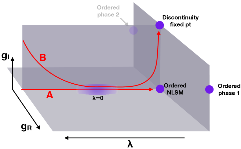
Figure 1: RG flows at $J_{c}$, i.e. with vanishing strongly relevant coupling $g_{R}=0$ (schematic). Flow line A: A hypothetical exactly $O(4)$-symmetric model is assumed to flow slowly through the pseudocritical region (blurred purple area), eventually reaching the ordered phase of the $O(4)$ sigma model. Flow line B: The coupling $g_{I}$ is effectively irrelevant in the pseudocritical regime, so the flow is attracted towards $g_{I}=0$. However the coupling is strongly relevant at the ordered fixed point of the nonlinear sigma model and ultimately it drives the flow to the discontinuity fixed point representing a trivial first order transition. There is an intermediate regime showing the properties of the ordered $O(4)$-symmetric sigma model.

A similar picture applies at the easy-plane Néel–VBS transition, despite the rather different microscopic symmetry. In easy-plane models on the square lattice there is a relevant perturbation $\sum_{a=1,2}X^{(2)}_{aa}$ driving the transition and typically two leading irrelevant perturbations allowed by the (different) microscopic symmetry wang2017deconfined . These are a higher-order anisotropy between Néel and VBS, and fourfold symmetry breaking for the VBS:

$$\delta\mathcal{L}=g_{I}^{(1)}\sum_{a,b=1,2}X_{aabb}+g_{I}^{(2)}\sum_{a=3,4}X_{aaaa}.$$ (7)

The $O(4)$ pseudocritical regime described below may also arise in $N_{f}=2$ QED₃. An important difference in that context is that perturbations built from $X^{(2)}$ and $X^{(4)}$ are forbidden by microscopic $SU(2)$ flavour symmetry tsmpaf06 ; wang2017deconfined , indicating that $O(4)$ is even more robust at long lengthscales than in the cases we discuss here.

Now let us consider how the renormalization group flows of a theory with a higher symmetry $G$ (here ${G=O(4)}$) may allow for an unconventional first order transition in a microscopic model without $G$ symmetry wang2017deconfined . We assume there is a flow-line in the $G$-symmetric parameter space along which the RG flow becomes very slow. Let us parameterize the flow line by $\lambda$, with $\lambda$ decreasing under the flow, and with the slow region of RG flows being close to $\lambda=0$. For a heuristic picture, we can imagine that this represents the flow of the coupling constant in the nonlinear sigma model above, with $\lambda>0$ corresponding to the region of small stiffness (large $g$) and $\lambda\rightarrow-\infty$ corresponding to the ordered fixed point at large stiffness ($g=0$).

‘Slow’ is a qualitative rather than a precise statement in the present context: its usefulness will ultimately be determined by comparing the following results with numerics. However the idea of pseudocriticality due to slow RG flows can be made precise in cases where we have a tuning parameter that controls the slowness of the RG flows. One example is the $Q$-state Potts model for small $\Delta^{2}\equiv Q-Q_{c}(d)$, where $Q_{c}(d)$ is the largest value of $Q$ for which the transition is continuous in $d$ dimensions baxterpotts ; nienhuispotts ; nauenbergscalapino ; cardynauenbergscalapino ; IinoDetecting2018 . Another is the $\mathrm{NCCP}^{n-1}$ model for small $\Delta^{2}\equiv d-d_{c}(n)$, where $d_{c}(n)$ is the largest value of $d$ for which the transition is continuous at a given $n$ DCPscalingviolations . In these examples the RG equations can be expanded systematically in $\Delta^{2}$ for small $\Delta^{2}$. When $\Delta^{2}\leq 0$ the transition is continuous. $\Delta^{2}\gtrsim 0$ is the ‘pseudocritical’ regime of interest, with a correlation length that is exponentially large in $1/\Delta$.

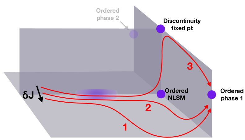
Figure 2: RG flows at small $\delta J=J-J_{c}$, showing three regimes in the idealized limit of an asymptotically weak first order transition (schematic). Here both $g_{R}$ and $g_{I}$ are nonzero. Flow line 1 comes close to the pseudocritical region before being driven away to the ordered phase by the relevant perturbation $g_{R}$. Flow line 2, closer to $J_{c}$, approaches the $O(4)$ long range ordered fixed point before being driven away. Flow line 3, extremely close to $J_{c}$: in this regime we see the asymptotic ‘universal’ properties of a standard first order transition.

Here we do not have a controlled $\Delta^{2}=0$ limit that preserves $O(4)$ symmetry, but to simplify the discussion, let us imagine that such a limit could be found in an appropriately deformed field theory. This limit yields several well-defined regimes of RG flow, giving the simplest illustration of the mechanism of interest. The physical model we study is not in the controllable limit of parametrically small $\Delta$ (regardless of whether an appropriate deformation of the field theory can be found). Therefore, rather than giving quantitative information about the RG flows in the physical model, the following discussion motivates a conjecture for the qualitative features of those flows. We will see below that the expectations from this conjecture appear to be borne out in simulations.

As discussed in wang2017deconfined ; cardynauenbergscalapino , for small $\Delta$ and $\lambda$ and in the vicinity of the flow line we have

$$\frac{\mathrm{d}\lambda}{\mathrm{d}\ln L} =-\lambda^{2}-a^{2}\Delta^{2}+\cdots$$ (8)

$$\frac{\mathrm{d}g_{R}}{\mathrm{d}\ln L} =+(y_{R}+c^{\prime}\lambda)g_{R}+\cdots,$$ (9)

$$\frac{\mathrm{d}g_{I}}{\mathrm{d}\ln L} =-(y_{I}+c\lambda)g_{I}+\cdots$$ (10)

where $a$, $c$ and $c^{\prime}$ are order one constants. Here, in addition to $\lambda$, we have included the most relevant coupling $g_{R}$ and the leading irrelevant one $g_{I}$ arising from $X^{(4)}$ (for simplicity we consider only one $g_{I}$). We have extracted a sign so that $y_{R}$ and $y_{I}$ are both positive, although $g_{I}$ is irrelevant.

First consider the case $g_{R}=g_{I}=0$. Integrating the above equation shows that for small $\Delta$ the lengthscale required for $\lambda$ to flow from a positive order 1 value to a negative order 1 value scales as

$$\xi_{\text{order}}\sim e^{\pi/{a\Delta}}.$$ (11)

We make the assumption that for large scales ${\ln L\gg\ln\xi_{\text{order}}}$ the flow is to the ordered fixed point of the sigma model in Eq. 4. This is consistent with the existence of a topological term in the sigma model since the topological term is irrelevant by power counting in the ordered phase. This flow is indicated by the flow line marked A in Fig. 1. The purple blur indicates the ‘slow’ regime close to $\lambda=0$.

Next consider the case $g_{I}\neq 0$, $g_{R}=0$. This is the flow line marked B in Fig. 1. Note that this corresponds to the microscopic model precisely at $J_{c}$. The perturbation $g_{I}$ is the leading effect of $O(4)$-breaking perturbations that are present in the microscopic model even at $J_{c}$.

The key point is that the $O(4)$–breaking perturbation $g_{I}$ decreases during the period of RG flow close to $\lambda=0$ (Eq. 10). Since the coupling is effectively irrelevant ($y_{I}>0$), and since $\xi_{\text{order}}$ is exponentially large in $\Delta$, by the time $\lambda$ is negative and of order one, the irrelevant coupling $g_{I}$ has become exponentially small: $g_{I}^{*}\sim e^{-\pi y_{I}/a\Delta}$ wang2017deconfined .

Therefore the flow ${\bf B}$ comes very close to the ordered fixed point of the NLSM. However, the anisotropy encoded in $g_{I}$ is relevant at this ordered fixed point. In the next stage of the RG flow the flow line B diverges from the ordered fixed point (Fig. 1). This is similar to phenomena in symmetry-breaking transitions with dangerously irrelevant anisotropies lou2007emergence .

Let us use the rescaled length coordinate $\tilde{x}=x/\xi_{\text{order}}$. Then an effective action in this regime is

$$\mathcal{S}=\int\mathrm{d}^{3}\tilde{x}\left[\frac{1}{2g_{\text{eff}}}\Big{(}\widetilde{\partial}{\bf n}\Big{)}^{2}+{g_{I}^{*}}O_{I}\right],$$ (12)

where $O_{I}$ is an anisotropy in the sigma model with the appropriate symmetry. Roughly speaking, the coupling $g_{\text{eff}}$ is of order one at the scale $\xi_{\text{order}}$, but grows rapidly under RG. Above, ${\bf n}^{2}=1$, but the lattice order parameters are related to this sigma model field by a power of $\xi_{\text{order}}$, since the magnitude of the order parameter decreases roughly like a power of $L$ in the pseudocritical regime.

In fact there are two separate lengthscales associated with the $O(4)$ breaking perturbation $g_{I}^{*}$, depending on whether we consider the probability distribution of the ordered moment (the zero-wavevector mode of the field), which is essentially a four-component vector of fixed length living on the three-sphere, or the Goldstone modes. The probability distribution for the zero mode becomes asymmetric at a scale

$$\xi_{\text{zero mode}}\sim\xi_{\text{order}}\times(g_{I}^{*})^{-\frac{1}{3}}\sim e^{\frac{\pi(1+y_{I}/3)}{a\Delta}}.$$ (13)

This is the lengthscale at which the contribution to the action (12) from the zero mode becomes of order 1, so that different orientations for the ordered moment are no longer approximately equally likely (this contribution is of order $g_{I}^{*}\times[L/\xi_{\text{order}}]^{3}$). The correlation functions of the Goldstone modes cross over from power law to exponential on a different scale that is in principle longer,

$$\xi_{\text{Goldstone}}\sim\xi_{\text{order}}\times(g_{I}^{*})^{-\frac{1}{2}}\sim e^{\frac{\pi(1+y_{I}/2)}{a\Delta}}.$$ (14)

(To see this note that in the rescaled coordinates $\tilde{x}$ the squared mass is simply proportional to $g_{I}^{*}$, since it is obtained by expanding Eq. 12 to quadratic order around one of the minima of the potential $O_{I}$.)

Finally, consider briefly the case where the microscopic model is perturbed away from the transition by ${\delta J=J-J_{c}}$. There are three different regimes, depending on the size of $\delta J$, that are illustrated in Fig. 2. The coupling $g_{R}$, which is initially small and proportional to $\delta J$, is growing at all stages of the RG flow. How small its initial value is will determine which fixed points in the $g_{R}=0$ plane the flow approaches before being driven away to one of the ordered phases at large (positive or negative) $g_{R}$, which here represent the Néel and VBS phases.

The above discussion is all in the idealized limit of small $\Delta$. In this limit there is a clean separation of scales between $\xi_{\text{order}}$ and $\xi_{\text{zero mode}}$ corresponding to the regime ‘close’ to the ordered fixed point of the symmetric sigma model (assuming we are sensitive to the probability distribution of the zero mode).

In the physical models, we do not expect this clean separation of scales, and we do not expect the detailed formulae in Eq. 10 to be accurate. Roughly speaking, the lengthscales relevant to us below are on the scales of, say, $10$ to $100$ so the relevant RG times are only of order one, because of the logarithmic relationship between length and RG time. So we are certainly not in the above limit where the flow of the coupling becomes extremely slow. But conversely, the exponential dependence of irrelevant variables on RG time means that accurate $O(4)$ can still emerge on these scales.

We will give evidence that the RG flows in the model we study have the basic qualitative features described above: an initial regime in which approximate $O(4)$ arises, with $O(4)$ ‘order’ at larger scales. (At present we cannot access large enough scales to see the subsequent flow away from the symmetric sigma model at $J_{c}$, although this may be possible.)

Before continuing, we note one caveat. The advantage of the present scenario, as an explanation for the following numerical results, is that it does not assume any fine-tuning of the microscopic parameters of the model beyond tuning of $J$ to $J_{c}$: the phenomenon is insensitive to the bare values of the irrelevant couplings $g_{I}$. But in principle an alternative way to flow close to the ordered $O(4)$ fixed point would be to fine-tune the bare parameters to be close to a tricritical qin2017duality ; JianEmergent2017 fixed point with two unstable directions, if an appropriate such fixed point, with $O(4)$ symmetry, happened to exist. Since this requires fine-tuning, we believe it is a less plausible explanation for our numerics than the scenario above.

III Model

The model we study is a simple modification of the loop model in DCPscalingviolations , so we summarise it briefly. This modification was initially proposed by sernaunpublished as a way to perturb the deconfined critical point to reach a first order transition. The model is an isotropic classical lattice model in three dimensions with cubic symmetry.

The relation to 2+1D deconfined criticality can be seen either from a transfer matrix construction or from an effective field theory DCPscalingviolations ; PhaseTransitionsCPNSigmaModel . The model has an exact $SO(3)$ spin symmetry which becomes manifest in a dual representation (with a local Néel vector ${\bm{\mathbf{N}}=(N_{x},N_{y},N_{z})}$ that is defined on each link of the lattice model). Heuristically, the loops can be thought of as wordlines of spinons in a spin-1/2 magnet, with two colours associated with the two spin directions.

The partition function is an ensemble of completely-packed loop configurations on the ‘3D L lattice’ cardy2010quantum shown in Fig. 3. (We use periodic boundary conditions, and measure lengths in units of the length of a link.) At each node $r$ the loops can be connected in two possible ways, with the two options labelled by an Ising-like variable $\phi_{r}=\pm 1$; the sign convention for $\phi$ is defined below. The configuration $\{\phi_{r}\}$ determines the geometry of the loops. Each loop can also take one of two colours, which are summed over in the partition function:

$$Z =\sum_{\{\phi\}}\sum_{\begin{subarray}{c}\text{loop}\\ \text{colours}\end{subarray}}e^{-E}.$$ (15)

Next we specify the energy $E$. The lattice is bipartite and each vertex $r$ is a member of either the $A$ or $B$ sublattice (blue and black in Fig. 3). There are interactions between nearest nodes on the same sublattice. In DCPscalingviolations these interactions were the same for the $A$ and $B$ lattices: we will refer to this here as the ‘symmetric’ model. The modification here is to have a different interaction for the $A$ and $B$ sublattices:

$$E=-J_{A}\sum_{\left\langle r,r^{\prime}\right\rangle\in A}\phi_{r}\phi_{r^{\prime}}-J_{B}\sum_{\left\langle r,r^{\prime}\right\rangle\in B}\phi_{r}\phi_{r^{\prime}}.$$ (16)

The $\phi$ variables on the two sublattices make up the two components of the VBS operator (see below). As usual in deconfined criticality, this operator also inserts a hedgehog defect in the Néel order parameter (this can be verified by computing the Berry phase associated with a hedgehog DCPscalingviolations in analogy to haldane ; readsachdevberryphase ).

The model has a phase in which the average loop length diverges: this is the Néel phase, with long range $SO(3)$-breaking order. This phase occurs for small $J$. The Néel 2-point function is related to the probability that two distant links lie on the same loop, or (as is trivially related) to the probability that two distant links are the same colour. The loop representation allows efficient calculation of Néel correlators. In the following we will use $N_{x}$ to denote the uniform (spatially averaged) Néel order parameter. See the Supplementary Material of emergentso5 for more detail on how to measure correlation functions.

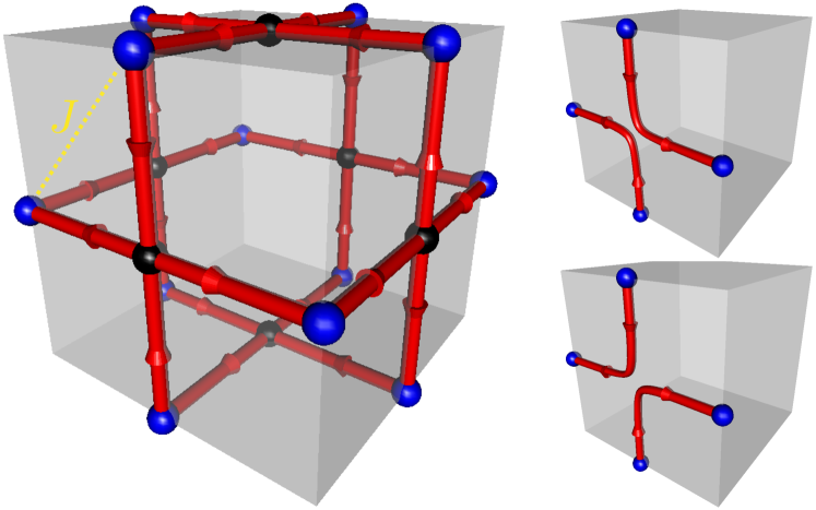
Figure 3: Left: Lattice structure of 3D L lattice. Nonintersecting loop configurations are obtained by choosing one of two possible pairings of links at each node $r$ (Right). There are interactions between nearest nodes on the A sublattice (shown in blue) of strength $J$ (indicated by dashed line). We set the interaction strength to zero for nodes on the $B$ sublattice (black).

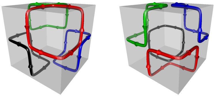
Figure 4: Two of the four equivalent configurations with minimal length loops (colours are only a guide to the eye). The configuration on the Left may be taken as the reference configuration to fix the sign convention for the $\phi$ variables. In both configurations shown, the $A$ nodes have $\phi_{x}=1$. The $B$ nodes have $\phi_{y}=1$ in the Left figure and $\phi_{y}=-1$ in the Right figure, so these configurations are $(\phi_{x},\phi_{y})=(1,1)$ and $(1,-1)$ respectively. We are interested in a phase transition at which $\varphi\equiv\phi_{x}$ orders while $\phi_{y}$ remains disordered. The sign of $\phi_{x}$ can be viewed as picking out a sublattice of cubes for the loops to ‘resonate’ around, see Fig. 5.

The model also permits VBS phases which break spatial symmetry and in which the loops are finite. First consider the symmetric model, $J_{A}=J_{B}$. At large enough $J_{A}=J_{B}$ the model is in a VBS phase that is four-fold degenerate. This degeneracy can be understood from the extreme limit of large $J$ in which all the loops are of the minimal length (six links). There are precisely four such states. To fix the sign convention of $\phi_{r}$, we pick an arbitrary one of these four states as a reference state, and declare $\phi_{r}=1$ for all $r$ in this state (Fig. 4).

The two components of the VBS order parameter are defined by $\phi_{r}$ for $r\in A$ and $r\in B$ respectively. The overall magnitude of the order parameter is

$$(\phi_{x},\phi_{y})=\frac{\sqrt{2}}{\text{no. sites}}\left(\sum_{r\in A}\phi_{r},\sum_{r\in B}\phi_{r}\right).$$ (17)

In the four extreme VBS states above (which are related by lattice symmetry) we have

$$(\phi_{x},\phi_{y})=\frac{1}{\sqrt{2}}(\pm 1,\pm 1).$$ (18)

The component $N_{z}$ of the Néel order parameter may be mapped to a variable $\chi_{\ell}$, living in the link $\ell$, whose value is $\pm 1$ depending on whether the link is red or blue emergentso5 . The spatially averaged order parameter is then ${N_{z}=\sum_{\ell}\chi_{\ell}/(\text{no. links})}$.

In the symmetric model the transition from Néel to VBS is at $J_{A}=J_{B}=0.088501(3)$. In this work we will fix $J_{B}$ to zero, in order to be far away from the symmetric critical point (avoiding crossover effects), and we will vary $J_{A}$ to access the phase transition between the Néel and VBS phases:

$$J_{A} \equiv J J_{B} =0\,.$$ (19)

We take $J>0$. Therefore $\phi_{x}$ is more strongly coupled than $\phi_{y}$. As $J$ is increased, there is a phase transition at which Néel order disappears, and $\phi_{x}$ orders. At this Néel-VBS phase transition, $\phi_{y}$ remains disordered (massive). This is the transition that we will study. The sign of the order parameter $\left\langle\phi_{x}\right\rangle$ can be viewed as picking out one of two sublattices of cubes for the loops to ‘resonate’ around, see Fig. 5 for a cartoon.

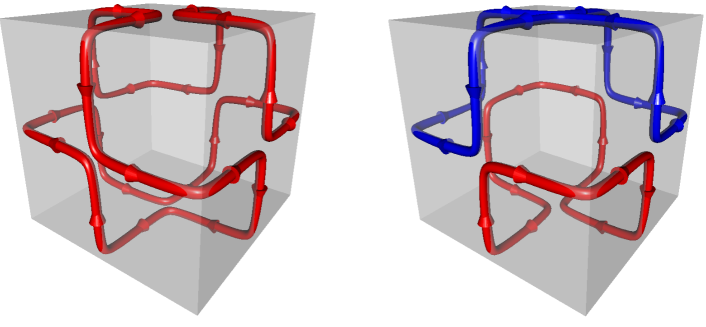
Figure 5: When $\phi_{x}$ is ordered, but $\phi_{y}$ is not, this picks out a sublattice of cubes. The figures show the case where $\phi_{x}=1$ and $\phi_{y}$ is arbitrary. In this extreme limit the loops live on the cubes with centres at $2(a,b,c)$ with ${a+b+c=\text{even}}$, such as the cube shown centred at the origin. For $\phi_{x}=-1$, the loops live on cubes with centres at $2(a,b,c)$ with ${a+b+c=\text{odd}}$ (the length of one link is taken to be 1).

If, starting in the VBS phase with $\left\langle\phi_{x}\right\rangle\neq 0$, we then increase $J_{B}$ sufficiently, we encounter another phase transition at which $\phi_{y}$ also orders. This is a conventional Ising transition which we will not be interested in. The full phase diagram for the model, close to the symmetric critical point, is shown in Fig. 6.

In Appendix A we show data for both components of $\phi$ at the transition of the model with $J_{B}=0$. This confirms that $\phi_{y}$ is a massive field with a short correlation length, and that for these parameters the model is ‘far’ from the symmetric critical point in the model with ${J_{A}=J_{B}}$: i.e. there is a strong asymmetry between $\phi_{x}$ and $\phi_{y}$ even at short scales. It is important to check this, because the critical point in the symmetric model is known to have a very accurate $SO(5)$ symmetry. If we studied a very weakly asymmetric model that was too close to this symmetric critical point, there would be an intermediate range of scales with approximate $SO(5)$, and $O(4)$ would be a trivial consequence of this higher symmetry. This is not the case here.

The order parameters that are involved in the phase transition of interest (indicated by the pink arrow in Fig. 6) are $\phi_{x}$ and $\bm{\mathbf{N}}$. To minimize subscripts we will write

$$\varphi\equiv\phi_{x}.$$ (20)

The order parameters can be arranged in a superspin $\bm{\mathbf{n}}$, Eq. 3. Since the normalization of the lattice order parameters is arbitrary, $\varphi$ must be rescaled by a fixed but nonuniversal constant in order for $\bm{\mathbf{n}}$ to have a chance of being invariant under $O(4)$ rotations.

Note that the relevant symmetry is $O(4)$ rather than $SO(4)$: improper rotations of ${\bf n}=(N_{x},N_{y},N_{z},\varphi)$ are allowed. A translation by two link lengths parallel to an axis is a microscopic example of an improper $O(4)$ rotation, as it changes the sign of $\varphi$ but not of $\bm{\mathbf{N}}$. [This translation also changes the sign of $\phi_{y}$, so in the symmetric model it is however a proper rotation within $SO(5)$.]

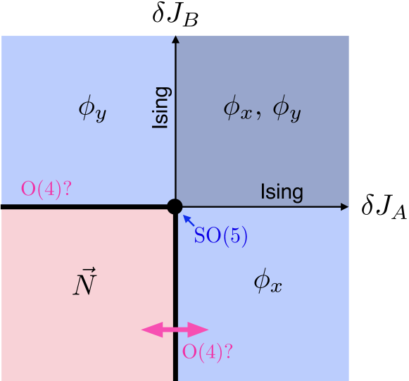
Figure 6: Schematic phase diagram of the model in Eq. 16 in the vicinity of the symmetric critical point at ${J_{A}=J_{B}\simeq 0.0885}$. The Néel phase and the three VBS phases are labelled by the order parameter(s) with a nonzero expectation value in the phase. We study the transition indicated by the pink arrow. However we study this transition relatively far from the symmetric critical point, in order to avoid crossover effects.

Before turning to numerical results, we briefly clarify our notation for the VBS order parameter, and contrast the present model with a square lattice quantum magnet with rectangular anisotropy in the couplings tsmpaf06 ; metlitski2017intrinsic .

Our convention for $\bm{\mathbf{\phi}}$ is such that the VBS-ordered states in the symmetric model ($J_{A}=J_{B}>J_{\text{critical}}$) are at $\bm{\mathbf{\phi}}\propto(\pm 1,\pm 1)$. If we temporarily redefine the order parameter by ${\bm{\mathbf{\phi}}^{\prime}=\frac{1}{\sqrt{2}}(\phi_{x}+\phi_{y},\phi_{x}-\phi_{y})}$, the ordered states are instead at $\bm{\mathbf{\phi}}^{\prime}\propto(\pm 1,0)$, $(0,\pm 1)$. This now matches the usual convention for columnar VBS ordered states in square lattice quantum magnets.

In this language, making $J_{A}$ slightly different from $J_{B}$, as above, introduces the term ${\phi_{x}^{2}-\phi_{y}^{2}\propto\phi_{x}^{\prime}\phi_{y}^{\prime}}$, which preserves symmetries under reflections across the lines ${\phi^{\prime}_{x}=\pm\phi^{\prime}_{y}}$. If we start in the VBS-ordered phase of the symmetric model and turn this perturbation on weakly, these symmetries ensure that there are still four degenerate ground states: this corresponds to the upper right quadrant of Fig. 6.

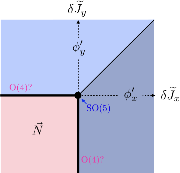
Figure 7: We contrast Fig. 6 with the phase diagram expected when a perturbation ${\delta\tilde{J}_{x}-\delta\tilde{J}_{y}}$, favouring two out of four of the VBS minima, is added to the critical point in the symmetric model (see text for notation). This perturbation is analogous to rectangular anisotropy in a square lattice quantum magnet at the Néel to columnar VBS transition, see text.

This should be contrasted with rectangular anisotropy in the square lattice magnet, which is analogous to a different perturbation of the Lagrangian, ${(\phi^{\prime}_{x})^{2}-(\phi^{\prime}_{y})^{2}}$, which instead preserves reflection symmetries across the lines $\phi^{\prime}_{x}=0$ and $\phi^{\prime}_{y}=0$. In the VBS ordered phase, turning this perturbation on immediately reduces the ground state degeneracy from four to two. The phase diagram for a model with rectangular anisotropy, perturbed away from the symmetric critical point by ${\delta\mathcal{L}=\delta\widetilde{J}_{x}(\phi^{\prime}_{x})^{2}+\delta\widetilde{J}_{y}(\phi^{\prime}_{y})^{2}}$, is shown in Fig. 7. The diagonal line is the four-fold degenerate VBS-ordered phase of the symmetric model.

Despite the different topologies of Figs. 6, 7, if there is indeed a quasiuniversal $O(4)$ regime that is accessible via an RG flow from the $SO(5)$ point, then we would expect to be able to access it in both models (at least close enough to the symmetric critical point) on the phase transition lines marked ‘$O(4)$?’ in Figs. 6, 7.

As discussed above, simulations of the phase transition close to the symmetric point would be complicated by additional crossover effects, so here we study a point on the phase transition line that is relatively far from the line $J_{A}=J_{B}$.

IV Numerical results

In Fig. 8 we show the Binder cumulants for the two order parameters close to the critical coupling,

$$J_{c}=0.0993916(10)$$ (21)

(our method for estimating $J_{c}$ is described below). At first glance these data for the Binder cumulants appear to show a continuous transition between phases with Néel and VBS order. Note the absence, on these scales, of the diverging positive peaks that would be expected for a conventional first order transition. We will argue that the transition is ultimately first order, but has a broad regime of lengthscales where it resembles an $O(4)$ spin flop transition. On this range of lengthscales, the Néel and VBS states are effectively related by a continuous rotational symmetry. This is quite different from a conventional first order transition, where, at $J_{c}$, the two competing phases are not even related by a discrete symmetry, and have (in the classical case) different energy and entropy.

We argue in three steps: first for the first-order nature of the transition, then for the presence of $O(4)$ symmetry, then for the presence of effective $O(4)$ long range order.

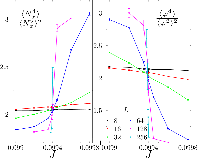
Figure 8: Binder cumulants $\langle N_{x}^{4}\rangle/\langle N_{x}^{2}\rangle^{2}$ (left panel) and $\langle\varphi^{4}\rangle/\langle\varphi^{2}\rangle^{2}$ (right panel) shown as a function of the coupling $J$, for several system sizes.

IV.1 Evidence for first order nature of transition

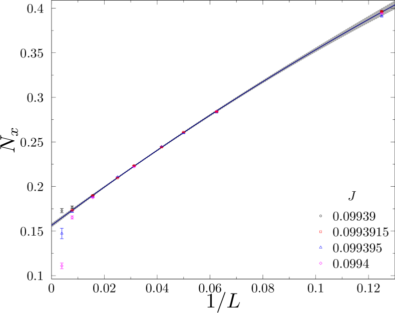
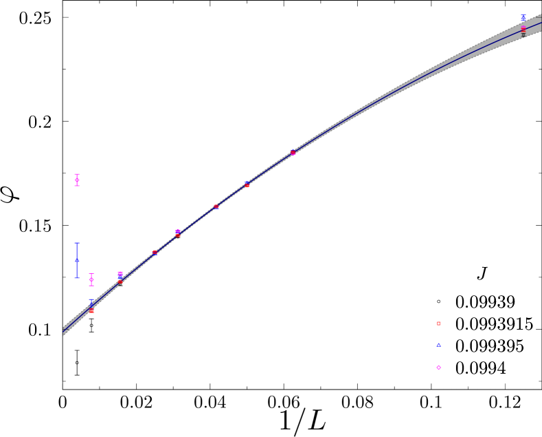
Figure 9: Order parameters $N_{x}$ and $\varphi$ as a function of $1/L$ for several values of $J$ close to $J_{\rm c}$ . Data points at $J=0.0993915$ are fitted to ${a+b/L+c/L^{2}}$, shown as a continuous line together with the shaded area corresponding to the statistical 95% confidence interval.

We first give evidence that the transition is first order rather than continuous. Since the transition is certainly not strongly first order, we cannot access the very large system sizes $L$ required to see conventional first order signatures such as double-peaked histograms for the energy. Instead we examine the size-dependence of the order parameters at $J_{c}$. We give evidence that as $L\rightarrow\infty$ both order parameters extrapolate to a nonzero value, indicating coexistence between the two phases at $J_{c}$, i.e. a first order transition.

The two panels in Fig. 9 show the Néel and VBS order parameters, $N_{x}\equiv\sqrt{\left\langle N_{x}^{2}\right\rangle}$ and $\varphi\equiv\sqrt{\left\langle\varphi^{2}\right\rangle}$, as a function of system size at four selected values of $J$ close to $J_{c}$. (Here the operator in the expectation value, e.g. $N_{x}$, is averaged over the system volume.) The continuous lines are fits to the form $a+b/L+c/L^{2}$ for the $J$ value closest to $J_{c}$ (shaded areas are 95% confidence intervals for these fits). Extrapolated values at $L=\infty$ are:

$$N_{x} =0.1562(14), \varphi =0.0987(14).$$ (22)

Fits to similar forms, including $a+bL^{-c}$, give compatible results, while putting the data on a log-log plot (Appendix A) shows that a power-law fit with $a=0$ is not good. Note that the numerical values in Eq. 22 are not expected to be the same for both order parameters, as they depend on the arbitrary normalizations of the lattice operators.

IV.2 Evidence for approximate $O(4)$ symmetry

If $O(4)$ symmetry emerges it fixes relations between various moments of the order parameters at $J_{c}$. We will give evidence for approximate symmetry under a subgroup of $O(4)$, whith is the $U(1)$ acting on $(N_{x},\varphi)$. (The $SO(3)$ acting on $\bm{\mathbf{N}}$ is an exact microscopic symmetry.) Given microscopic symmetries, an additional emergent symmetry rotating $N_{x}$ into $\varphi$ is sufficient to generate the full emergent internal $O(4)$ symmetry.

First we examine the ratio between the order parameters, ${\varphi/N_{x}\equiv\sqrt{\left\langle\varphi^{2}\right\rangle/\left\langle N_{x}^{2}\right\rangle}}$, in Fig. 10. In the presence of emergent symmetry, this ratio should be $L$-independent at $J_{c}$ (see e.g. emergentso5 ; sreejith2018emergent ), yielding a crossing of curves for different $L$. Fig. 10 indeed shows a well-defined crossing if the smallest size, $L=8$, is excluded, despite the fact that the order parameters are individually varying strongly with $L$.

The $J$-values of the crossings between consecutive $L$s are shown in the inset to Fig. 10. A weighted average of these crossings yields the estimate $J_{c}=0.0993918(7)$ for the transition point.

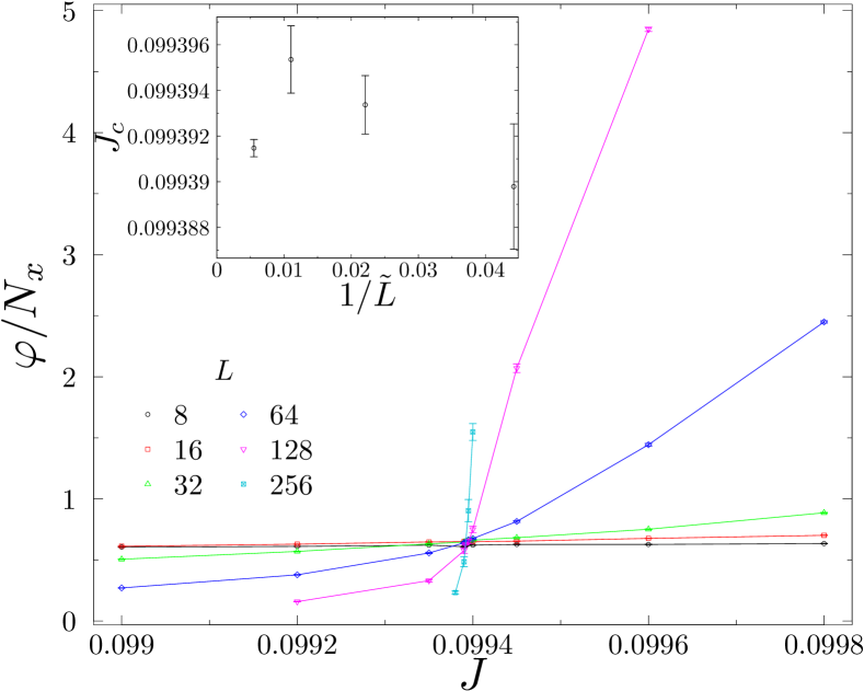
Figure 10: Main panel: curves of the ratio $\sqrt{\left\langle\varphi^{2}\right\rangle/\left\langle N_{x}^{2}\right\rangle}$ as function of the coupling $J$, showing a clear crossing close to $J\approx 0.0993915$. Inset: values of $J$ at the crossing points between two consecutive system sizes, $L_{1}$ and $L_{2}$, as a function of the inverse of the geometric mean $\tilde{L}=\sqrt{L_{1}L_{2}}$.

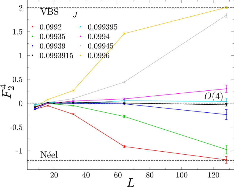
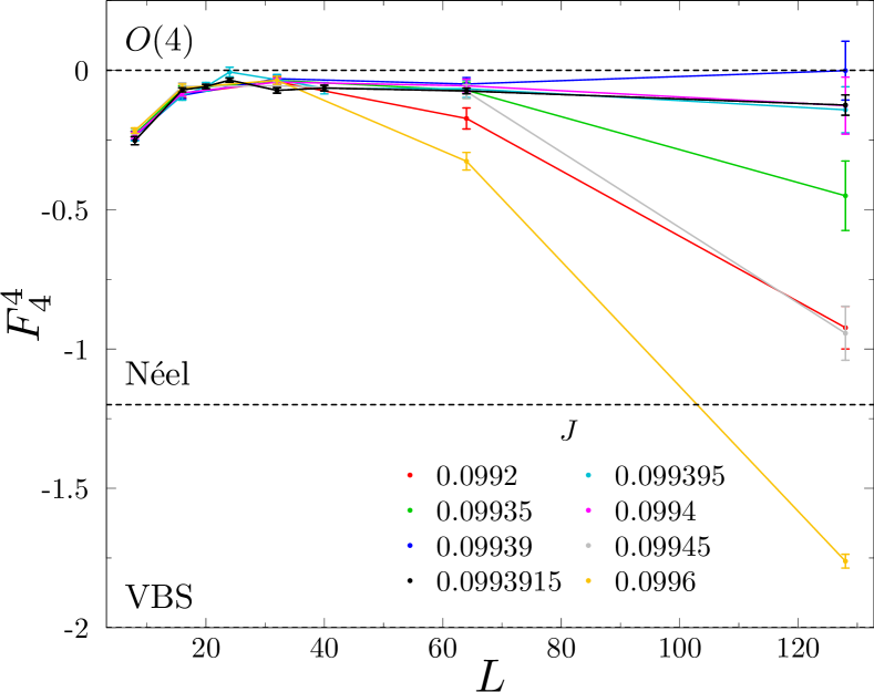
Figure 11: Moments $F_{2}^{4}$ and $F_{4}^{4}$ as a function of the system size for several values of $J$. Dashed lines correspond to expected values in the Néel phase, at an $O(4)$-symmetric point, and in the VBS ($Z_{2}$) phase.

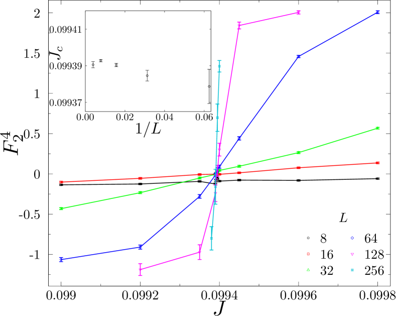
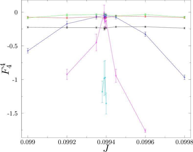
Figure 12: Moments $F_{2}^{4}$ and $F_{4}^{4}$ as a function of $J$. Note that in the second panel, the peak in $F_{4}^{4}$ for $L=256$ is probably hidden because its width is smaller than the separation between the data points. Inset: values of $J$ at which $F_{2}^{4}$ is equal to 0, shown versus $1/L$. The weighted average gives an estimate of $J_{c}$.

Next we examine some moments of the joint probability distribution for $N_{x}$ and $\varphi$ emergentso5 ; sreejith2018emergent . Let ${(N_{x},\varphi)=r(\cos\theta,\sin\theta)}$, and let $F^{a}_{\ell}=\left\langle r^{a}\cos(\ell\theta)\right\rangle$. This should vanish for $\ell>0$ in the presence of $U(1)$ symmetry relating these two order parameter components.

In Figs. 11 and 12 we show

$$F_{2}^{4}=\left\langle\tilde{N}_{x}^{4}-\tilde{\varphi}^{4}\right\rangle,\quad F_{4}^{4}=\left\langle\tilde{N}_{x}^{4}-6\tilde{N}_{x}^{2}\tilde{\varphi}^{2}+\tilde{\varphi}^{4}\right\rangle.$$ (23)

Here $\tilde{N}_{x}=N_{x}/\sqrt{\left\langle N_{x}^{2}\right\rangle}$ and $\tilde{\varphi}=\varphi/\sqrt{\left\langle\varphi^{2}\right\rangle}$ are the order parameters normalized to have unit variance.

In Fig. 11 the quantities $F_{2}^{4}$ and $F_{4}^{4}$ are shown as a function of system size for various $J$ values close to $J_{c}$. Strikingly, at ${J=0.0993915}$ (the value closest to $J_{c}$) $F_{2}^{4}$ is zero to within errors for system sizes $16\leq L\leq 128$. $F_{4}^{4}$ approaches zero quite closely, consistent with approximate $O(4)$. There appears to be a small but measurable difference from zero over this size range, indicating that $O(4)$ is not perfect.

$F_{2}^{4}$ and $F_{4}^{4}$ are also plotted as a function of $J$ in Fig. 12. The $J$ values of the crossings of $F_{2}^{4}$ with zero, which are shown in the inset of Fig. 12, can be used to obtain a different estimate of the transition point, which is ${J_{c}=0.0993916(10)}$. This is the estimate in Eq. 21.

The curves for $F_{4}^{4}$ in the lower panel of Fig. 12 feature a peak at $J_{c}$ with a maximum close to zero. This peak gets abruptly narrower with increasing system size. For ${L=256}$, the width of this peak may lie within the unsampled interval $0.099390<J<0.099395$ (we do not have data for $J=0.0993915$ for this size).

IV.3 Evidence for $O(4)$–ordered regime

We now give evidence that at the longest scales we can access the system is in a regime which is described approximately by the $O(4)$ sigma model in its ordered or Goldstone phase, as discussed in Sec. II.

A first indication of this is that for $L\sim 128$ the order parameter values are fairly close to their extrapolated $L=\infty$ values (Sec. IV.1), while at the same time the moment ratios are close to the $O(4)$ values. This is consistent with being in the $O(4)$-ordered regime. It is not consistent with a standard critical regime (where the order parameters would be scaling to zero with $L$)  and it is not consistent with a standard first order regime (where there would be no $O(4)$ symmetry).

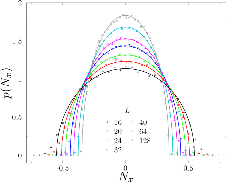
Figure 13: Probability distribution of $N_{x}$ for several system sizes at $J=0.0993915$. Continuous lines are fits to Eq. 25 with $R$ as the only parameter (the fitted region is with $p(N_{x})>0.15$). The extrapolated value of the order parameter in Eq. 22 corresponds to a semicircle with peak height of $2.0$.

For a concrete check, we compare the probability distribution of a component of the order parameter with that expected for the sigma model in the ordered phase. Deep in the ordered phase, the 4-component order parameter can be treated as spatially constant, and has a uniform probability distribution on the sphere

$$|{\bf n}|^{2}=R^{2}.$$ (24)

Integrating out 3 components gives the probability distribution for a single component, which is a semicircle:

$$P(n_{1})=\frac{2}{\pi R^{2}}\sqrt{R^{2}-n_{1}^{2}}.$$ (25)

This semicircle distribution is a hallmark of $O(4)$ order.

First, the probability distribution for $N_{x}$ is shown in Fig. 13 for several system sizes. We fit each curve to Eq. 25, with $R$ as the only parameter (continuous lines). The extrapolated $L=\infty$ value of the order parameter in Eq. 22 would correspond to the the height of the peak of the curve in Fig. 13 being $\sim 2.0$.

In Fig. 14 we show the probability distributions for the normalized order parameter components, $\tilde{N}_{x}$ and $\tilde{\varphi}$ with variance 1. We see that the shape of the probability distribution changes more weakly than the overall width. The expected semicircle form is shown as a black line (without any fitting parameter, since the variance is now fixed). Error bars are smaller for $N_{x}$ than for $\varphi$.

While deviations from the semicircle are apparent for the smaller sizes, the distributions for $L=64$ and $L=128$ match extremely well to the semicircle. The amount of weight in the tails $|\tilde{N}_{x}|>2$ is clearly decreasing as $L$ is increased, as expected from the semicircle form which has a bounded support.

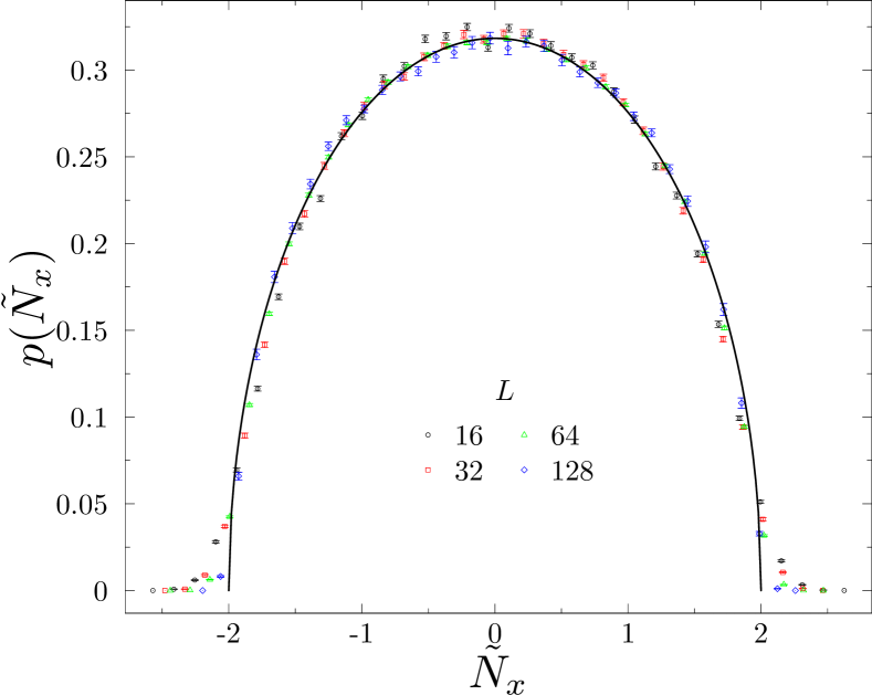
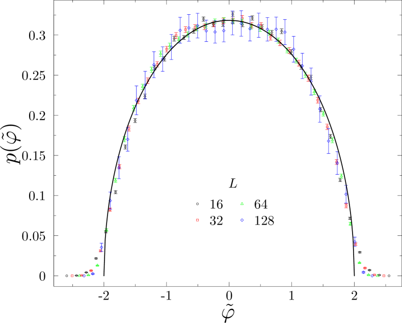
Figure 14: Probability distribution of the normalized $\tilde{N}=N_{x}/\sqrt{\left\langle N_{x}^{2}\right\rangle}$ and $\tilde{\varphi}=\varphi/\sqrt{\left\langle\varphi^{2}\right\rangle}$ for several system sizes. Curves show semicircle distribution with radius $R=2$.

Finally, for a more quantitative analysis, we compare cumulants of the order parameters with the values expected from the symmetric $O(4)$ sigma model in its ordered phase. Consider the cumulants (recall that $\tilde{N}_{x}$ is normalized to have unit variance)

$$C_{4} =\left\langle\tilde{N}_{x}^{4}\right\rangle-3\left\langle\tilde{N}_{x}^{2}\right\rangle^{2},$$ (26)

$$C_{6} =\left\langle\tilde{N}_{x}^{6}\right\rangle-15\left\langle\tilde{N}_{x}^{4}\right\rangle\left\langle\tilde{N}_{x}^{2}\right\rangle+30\left\langle\tilde{N}_{x}^{2}\right\rangle^{3},$$ (27)

and similarly for $\tilde{\varphi}$. In the $O(4)$ ordered regime, we expect from Eq. 25:

$$C_{4} =-1, C_{6} =5,$$ (28)

for both $N_{x}$ and $\varphi$. These values are very different from those that would be obtained for a Gaussian distribution (zero) or at a conventional first order transition.

In Fig. 15 we show these cumulants at $J=J_{c}$ as a function of the inverse of the system size, for both order parameters. Both $C_{4}$ and $C_{6}$ are relatively close to the values expected from the ordered sigma model even for the smaller sizes, and for the larger sizes they are very close. This suggests that the system at $J_{c}$ is well described by the ordered phase of the symmetric sigma model for $L\sim 128$ and even $L\sim 64$, despite the fact that the ordered moment at $L=64$ is still quite far from its extrapolated value (Fig. 9).

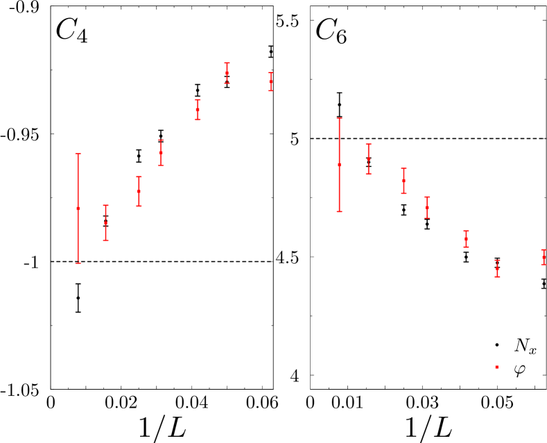
Figure 15: Cumulants $C_{4}$ and $C_{6}$ at $J=0.0993915$ as function of the inverse of the system size, $1/L$. Dashed lines are the expected values for the $O(4)$-symmetric ordered sigma model, $C_{4}=-1$ and $C_{6}=5$.

V Outlook

We have exhibited a phase transition with emergent $O(4)$ symmetry and a regime where the $O(4)$ vector is effectively ordered. This symmetry is only expected to be approximate, and therefore the description using the long-range ordered $O(4)$ sigma model is also only approximate even in the relevant range of length scales. However, the usefulness of this concept in organizing our understanding of this phase transition is clear. We have shown that it allows us to predict various ‘quasiuniversal’ features with good accuracy. As a zeroth order description for length scales of order, say, $100$, the ‘$O(4)$ spin flop’ description is clearly far more useful than standard expectations for first order transitions, which are strongly violated because of the effective continuous symmetry relating the two phases at coexistence.

The description of the data using the sigma model description could be further improved by considering Goldstone fluctuation corrections, as well as the leading weak anisotropies in the Lagrangian. Many other quantities, such as two-point functions or off-critical scaling forms, could also be understood with this approach.

The phenomenon we have argued for in the present model is likely to be more general wang2017deconfined . Examples may exist with a range of emergent symmetry groups $G$, and for a given $G$, there will be many different possibilities for the (smaller) microscopic symmetry group.

The present $O(4)$ regime may also appear in several other contexts. From the renormalization group picture one would naively expect that at large scales the ‘easy-plane’ Néel-VBS transition qin2017duality ; zhang2018continuous ; kukloveasyplane ; kragseteasyplane ; kauleasyplane1 ; kauleasyplane2 behaves similarly to the model discussed here tsmpaf06 ; metlitski2017intrinsic ; wang2017deconfined . (The easy plane transition involves competition between a two-component Néel order parameter and a two-component VBS order parameter.) However, recent work has argued that this transition can be continuous rather than first order qin2017duality ; zhang2018continuous . This should be understood better. The classical 3D dimer model, with appropriate anisotropy, is another platform that could be used to study the physics of the easy-plane $\mathrm{NCCP}^{1}$ model Chenetal ; sreejith2018emergent .

The regime demonstrated here should also be looked for in two-flavour QED₃, and is an alternative possibility to flow to a scale-invariant fixed point argued for previously on numerical grounds qedcft . (The effect of $O(4)$-breaking perturbations within the $O(4)$–ordered phase is expected to be much weaker in that context wang2017deconfined .)

A long-range-ordered $SO(5)$ regime may occur for deconfined criticality with 5 components, for example $SU(2)$-symmetric magnets at the Néel-VBS transition on the square lattice wang2017deconfined . Existing data shows features that seem compatible with a pseudocritical regime, for example drifting exponents that at large size tend to values that are incompatible with the exponents of a conformal fixed point DCPscalingviolations ; SimmonsDuffinSO(5) ; Nakayama ; PolandReview , at least if conventional finite-size scaling is assumed. However if the flow is eventually to the long-range-ordered state, the lengthscale needed to see this regime is very large and appears to be beyond the reach of current simulations DCPscalingviolations . Indeed on the presently accessible lengthscales the $SO(5)$ symmetry in various models resembles an exact symmetry of the infrared theory emergentso5 ; sreejith2018emergent .

In the future it will be useful to quantify more precisely the the accuracy of the emergent approximate $O(4)$ symmetry in the model studied here as a function of $L$. A more careful comparison with expectations from the ordered sigma model, taking finite size effects into account, as well as the effects of finite ${J-J_{c}}$, would also be enlightening. Simulations at larger $L$ might be able to probe the eventual flow away from the symmetric sigma model (Fig. 2).

Finally, here we have focussed only on the critical point at $J_{A}=J_{c}$, $J_{B}=0$. It will also be important to investigate the transition both in the presumably more strongly first-order regime at negative $J_{B}$ and in the presumably more weakly first-order regime at larger $J_{B}$. In Sec. II we noted an alternative scenario in which approximate $O(4)$ arises because the model is by accident fine-tuned close to an unstable $O(4)$–invariant tricritical point. We have argued this is unlikely as it would require fine-tuning (and an appropriate such fixed point may not exist). This could be checked directly by checking that the $O(4)$ ordered regime is robust against small changes of the microscopic parameters.

Related Work: After completion of this work we became aware of a numerical study of a deformed $JQ$ model by Zhao et al. zhao2018symmetry . That model also has a transition with 4 order parameter components, and the authors also find a first order transition with emergent $O(4)$ symmetry, as here.

Appendix A Comparison of two VBS components

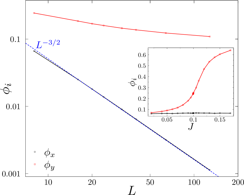
Figure 16: Main panel: we show the two components of $\phi$ (see Sec. III) as a function of system size at $J=0.0993915$ (close to $J_{c})$. Note the log-log scale. The definition is ${\phi_{i}=\sqrt{\left\langle\phi_{i}^{2}\right\rangle}}$, where the operator inside the expectation value is averaged over the full system volume. First, observe that for our choice of couplings (Eq. 19) there is a very strong asymmetry between $\varphi=\phi_{x}$ and $\phi_{y}$ even at small scales. The magnitude of $\phi_{y}$ decreases as $L^{-3/2}$ (dashed line), as expected for a massive field. This shows that the $O(4)$ symmetry we find is not just a consequence of proximity to the $SO(5)$ invariant critical (or pseudocritical) point in the symmetric model with ${J_{A}=J_{B}}$. Second, note that the log-log plot for $\varphi=\phi_{x}$ (red line) is not straight, showing that the power law scaling that would be expected at a critical point does not apply here. Instead, $\varphi$ extrapolates to a finite value as $L\rightarrow\infty$ (Sec. IV.1). Inset: we show the two components of $\phi$ as a function of $J$ in a small system ($L=8$). Again the strong asymmetry between $\varphi=\phi_{x}$, which orders at the transition, and $\phi_{y}$, which remains massive, is apparent.

In Fig. 16 we show the two components of the VBS order parameter in Eq. 17, $\phi_{x}$ and $\phi_{y}$, both as a function of $L$ at $J_{c}$, and as a function of $J$ for $L=8$. The figure shows that at the transition $\phi_{y}$ is a massive field with a short correlation length, and that there is a strong asymmetry between $\phi_{x}$ and $\phi_{y}$ even at short scales. This confirms that the coupling values we have chosen (i.e. $J_{B}=0$) are sufficiently far from the symmetric critical point with $J_{A}=J_{B}$. The symmetric critical point has very accurate $SO(5)$ symmetry. If we studied a weakly asymmetric model (i.e. $J_{A}-J_{B}$ too small) then there would be an intermediate range of scales with approximate $SO(5)$, and we would see $O(4)$ as a trivial consequence of this. It is clear from Fig. 16 that this is not the explanation for the $O(4)$ that we see.

References

- [1] T. Senthil, Ashvin Vishwanath, Leon Balents, Subir Sachdev, and Matthew P. A. Fisher. Deconfined quantum critical points. Science, 303:1490, 2004.
- [2] T. Senthil, Leon Balents, Subir Sachdev, Ashvin Vishwanath, and Matthew P. A. Fisher. Quantum criticality beyond the landau-ginzburg-wilson paradigm. Phys. Rev. B, 70:144407, Oct 2004.
- [3] Anders W. Sandvik. Evidence for deconfined quantum criticality in a two-dimensional heisenberg model with four-spin interactions. Phys. Rev. Lett., 98:227202, Jun 2007.
- [4] Roger G. Melko and Ribhu K. Kaul. Scaling in the fan of an unconventional quantum critical point. Phys. Rev. Lett., 100:017203, Jan 2008.
- [5] Jie Lou, Anders W. Sandvik, and Naoki Kawashima. Antiferromagnetic to valence-bond-solid transitions in two-dimensional heisenberg models with multispin interactions. Phys. Rev. B, 80:180414, Nov 2009.
- [6] Argha Banerjee, Kedar Damle, and Fabien Alet. Impurity spin texture at a deconfined quantum critical point. Phys. Rev. B, 82:155139, Oct 2010.
- [7] Anders W. Sandvik. Continuous quantum phase transition between an antiferromagnet and a valence-bond solid in two dimensions: Evidence for logarithmic corrections to scaling. Phys. Rev. Lett., 104:177201, Apr 2010.
- [8] Kenji Harada, Takafumi Suzuki, Tsuyoshi Okubo, Haruhiko Matsuo, Jie Lou, Hiroshi Watanabe, Synge Todo, and Naoki Kawashima. Possibility of deconfined criticality in su() heisenberg models at small . Phys. Rev. B, 88:220408, Dec 2013.
- [9] F-J Jiang, M Nyfeler, S Chandrasekharan, and U-J Wiese. From an antiferromagnet to a valence bond solid: evidence for a first-order phase transition. Journal of Statistical Mechanics: Theory and Experiment, 2008(02):P02009, 2008.
- [10] Kun Chen, Yuan Huang, Youjin Deng, A. B. Kuklov, N. V. Prokof’ev, and B. V. Svistunov. Deconfined criticality flow in the heisenberg model with ring-exchange interactions. Phys. Rev. Lett., 110:185701, May 2013.
- [11] A.B. Kuklov, N. V. Prokof’ev, B.V. Svistunov, and M. Troyer. Deconfined criticality, runaway flow in the two-component scalar electrodynamics and weak first-order superfluid-solid transitions. Annals of Physics, 321(7):1602 – 1621, 2006.
- [12] A. B. Kuklov, M. Matsumoto, N. V. Prokof’ev, B. V. Svistunov, and M. Troyer. Deconfined criticality: Generic first-order transition in the su(2) symmetry case. Phys. Rev. Lett., 101:050405, Aug 2008.
- [13] Ribhu K. Kaul and Anders W. Sandvik. Lattice model for the néel to valence-bond solid quantum phase transition at large . Phys. Rev. Lett., 108:137201, Mar 2012.
- [14] Hui Shao, Wenan Guo, and Anders W. Sandvik. Quantum criticality with two length scales. Science, 352(6282):213–216, 2016.
- [15] Jonathan D’Emidio and Ribhu K. Kaul. First-order superfluid to valence-bond solid phase transitions in easy-plane magnets for small . Phys. Rev. B, 93:054406, Feb 2016.
- [16] Yan Qi Qin, Yuan-Yao He, Yi-Zhuang You, Zhong-Yi Lu, Arnab Sen, Anders W Sandvik, Cenke Xu, and Zi Yang Meng. Duality between the deconfined quantum-critical point and the bosonic topological transition. Physical Review X, 7(3):031052, 2017.
- [17] Xue-Feng Zhang, Yin-Chen He, Sebastian Eggert, Roderich Moessner, Frank Pollmann, et al. Continuous easy-plane deconfined phase transition on the kagome lattice. Physical review letters, 120(11):115702, 2018.
- [18] Adam Nahum, J. T. Chalker, P. Serna, M. Ortuño, and A. M. Somoza. Deconfined quantum criticality, scaling violations, and classical loop models. Phys. Rev. X, 5:041048, Dec 2015.
- [19] Adam Nahum, P. Serna, J. T. Chalker, M. Ortuño, and A. M. Somoza. Emergent so(5) symmetry at the néel to valence-bond-solid transition. Phys. Rev. Lett., 115:267203, Dec 2015.
- [20] GJ Sreejith, Stephen Powell, and Adam Nahum. Emergent so (5) symmetry at the columnar ordering transition in the classical cubic dimer model. Physical Review Letters, 122(8):080601, 2019.
- [21] G. J. Sreejith and Stephen Powell. Scaling dimensions of higher-charge monopoles at deconfined critical points. Phys. Rev. B, 92:184413, Nov 2015.
- [22] Chong Wang, Adam Nahum, Max A Metlitski, Cenke Xu, and T Senthil. Deconfined quantum critical points: symmetries and dualities. Physical Review X, 7(3):031051, 2017.
- [23] T. Senthil and Matthew P. A. Fisher. Competing orders, nonlinear sigma models, and topological terms in quantum magnets. Phys. Rev. B, 74:064405, Aug 2006.
- [24] Akihiro Tanaka and Xiao Hu. Many-body spin berry phases emerging from the -flux state: Competition between antiferromagnetism and the valence-bond-solid state. Phys. Rev. Lett., 95:036402, Jul 2005.
- [25] Hidemaro Suwa, Arnab Sen, and Anders W. Sandvik. Level spectroscopy in a two-dimensional quantum magnet: Linearly dispersing spinons at the deconfined quantum critical point. Phys. Rev. B, 94:144416, Oct 2016.
- [26] David Poland, Slava Rychkov, and Alessandro Vichi. The conformal bootstrap: Theory, numerical techniques, and applications. Reviews of Modern Physics, 91(1):015002, 2019.
- [27] Olexei I Motrunich and Ashvin Vishwanath. Emergent photons and transitions in the o (3) sigma model with hedgehog suppression. Physical Review B, 70(7):075104, 2004.
- [28] Stephen Powell and J. T. Chalker. Su(2)-invariant continuum theory for an unconventional phase transition in a three-dimensional classical dimer model. Phys. Rev. Lett., 101:155702, Oct 2008.
- [29] D. Charrier, F. Alet, and P. Pujol. Gauge theory picture of an ordering transition in a dimer model. Phys. Rev. Lett., 101:167205, Oct 2008.
- [30] Gang Chen, Jan Gukelberger, Simon Trebst, Fabien Alet, and Leon Balents. Coulomb gas transitions in three-dimensional classical dimer models. Phys. Rev. B, 80:045112, Jul 2009.
- [31] Stephen Powell and J. T. Chalker. Classical to quantum mapping for an unconventional phase transition in a three-dimensional classical dimer model. Phys. Rev. B, 80:134413, 2009.
- [32] Snir Gazit, Fakher F Assaad, Subir Sachdev, Ashvin Vishwanath, and Chong Wang. Confinement transition of gauge theories coupled to massless fermions: emergent qcd and symmetry. arXiv preprint arXiv:1804.01095, 2018.
- [33] S. Kragset, E. Smørgrav, J. Hove, F. S. Nogueira, and A. Sudbø. First-order phase transition in easy-plane quantum antiferromagnets. Phys. Rev. Lett., 97:247201, Dec 2006.
- [34] Jonathan D?Emidio and Ribhu K Kaul. New easy-plane cpn-1 fixed points. Physical review letters, 118(18):187202, 2017.
- [35] Olexei I Motrunich and Ashvin Vishwanath. Comparative study of higgs transition in one-component and two-component lattice superconductor models. arXiv preprint arXiv:0805.1494, 2008.
- [36] Scott Geraedts and Olexei I. Motrunich. Lattice realization of a bosonic integer quantum hall state–trivial insulator transition and relation to the self-dual line in the easy-plane nccp1 model. Phys. Rev. B, 96:115137, Sep 2017.
- [37] Scott D. Geraedts and Olexei I. Motrunich. Monte carlo study of a system with -statistical interaction. Phys. Rev. B, 85:045114, Jan 2012.
- [38] Max A Metlitski and Ryan Thorngren. Intrinsic and emergent anomalies at deconfined critical points. Physical Review B, 98(8):085140, 2018.
- [39] Toshihiro Sato, Martin Hohenadler, and Fakher F Assaad. Dirac fermions with competing orders: Non-landau transition with emergent symmetry. Physical review letters, 119(19):197203, 2017.
- [40] Fa Wang, Steven A Kivelson, and Dung-Hai Lee. Nematicity and quantum paramagnetism in fese. Nature Physics, 11:959, 2015.
- [41] Zohar Komargodski, Tin Sulejmanpasic, and Mithat Unsal. Walls, anomalies, and (de)confinement in quantum anti-ferromagnets. Phys. Rev. B, 97:054418, 2018.
- [42] A. Karch and D. Tong. Particle-Vortex Duality from 3D Bosonization. Physical Review X, 6(3):031043, July 2016.
- [43] Cenke Xu and Yi-Zhuang You. Self-dual quantum electrodynamics as boundary state of the three-dimensional bosonic topological insulator. Phys. Rev. B, 92:220416, Dec 2015.
- [44] Po-Shen Hsin and Nathan Seiberg. Level/rank duality and chern-simons-matter theories. Journal of High Energy Physics, 2016(9):95, 2016.
- [45] Chao-Ming Jian, Alex Rasmussen, Yi-Zhuang You, and Cenke Xu. Emergent symmetry and tricritical points near the deconfined quantum critical point. arXiv preprint arXiv:1708.03050, 2017.
- [46] Nikhil Karthik and Rajamani Narayanan. Flavor and topological current correlators in parity-invariant three-dimensional qed. Phys. Rev. D, 96:054509, 2017.
- [47] R J Baxter. Potts model at the critical temperature. Journal of Physics C: Solid State Physics, 6(23):L445, 1973.
- [48] B. Nienhuis, A. N. Berker, Eberhard K. Riedel, and M. Schick. First- and second-order phase transitions in potts models: Renormalization-group solution. Phys. Rev. Lett., 43:737–740, Sep 1979.
- [49] M. Nauenberg and D. J. Scalapino. Singularities and scaling functions at the potts-model multicritical point. Phys. Rev. Lett., 44:837–840, Mar 1980.
- [50] John L. Cardy, M. Nauenberg, and D. J. Scalapino. Scaling theory of the potts-model multicritical point. Phys. Rev. B, 22:2560–2568, Sep 1980.
- [51] S Iino, S Morita, A W Sandvik, and N Kawashima. Detecting signals of weakly first-order phase transitions in two-dimensional potts models. arXiv preprint arXiv:1801.02786, 2017.
- [52] H. Gies and J. Jaeckel. Chiral phase structure of qcd with many flavors. The European Physical Journal C - Particles and Fields, 46(2):433–438, 2006.
- [53] David B. Kaplan, Jong-Wan Lee, Dam T. Son, and Mikhail A. Stephanov. Conformality lost. Phys. Rev. D, 80:125005, Dec 2009.
- [54] Jens Braun, Holger Gies, Lukas Janssen, and Dietrich Roscher. Phase structure of many-flavor . Phys. Rev. D, 90:036002, Aug 2014.
- [55] S Giombi, I R Klebanov, and G Tarnopolsky. Conformal qed d, f-theorem and the expansion. J. Phys. A, 49(13):135403, 2016.
- [56] I F Herbut. Chiral symmetry breaking in three-dimensional quantum electrodynamics as fixed point annihilation. Phys. Rev. D, 94:025036, 2016.
- [57] S Gukov. Rg flows and bifurcations. Nuclear Physics B, 919:583–638, 2017.
- [58] Adam Nahum, J. T. Chalker, P. Serna, M. Ortuño, and A. M. Somoza. Phase transitions in three-dimensional loop models and the sigma model. Phys. Rev. B, 88:134411, Oct 2013.
- [59] D. Simmons-Duffin. unpublished.
- [60] Yu Nakayama and Tomoki Ohtsuki. Necessary condition for emergent symmetry from the conformal bootstrap. Phys. Rev. Lett., 117:131601, Sep 2016.
- [61] N. Karthik and R. Narayanan. Scale invariance of parity-invariant three-dimensional QED. Phys. Rev. D, 94(6):065026, September 2016.
- [62] Jie Lou, Anders W Sandvik, and Leon Balents. Emergence of u(1) symmetry in the 3d xy model with anisotropy. Physical review letters, 99(20):207203, 2007.
- [63] Pablo Serna, Ribhu Kaul, and Anders Sandvik. Unpublished.
- [64] John Cardy. Quantum network models and classical localization problems. International Journal of Modern Physics B, 24(12n13):1989–2014, 2010.
- [65] FDM Haldane. O (3) nonlinear model and the topological distinction between integer-and half-integer-spin antiferromagnets in two dimensions. Physical review letters, 61(8):1029, 1988.
- [66] N Read and Subir Sachdev. Valence-bond and spin-peierls ground states of low-dimensional quantum antiferromagnets. Physical review letters, 62(14):1694, 1989.
- [67] Bowen Zhao, Phillip Weinberg, and Anders W Sandvik. Symmetry-enhanced discontinuous phase transition in a two-dimensional quantum magnet. Nature Physics, page 1, 2019.