Robust nonlinear processing of active array data in inverse scattering via truncated reduced order models

Abstract

We introduce a novel algorithm for nonlinear processing of data gathered by an active array of sensors which probes a medium with pulses and measures the resulting waves. The algorithm is motivated by the application of array imaging. We describe it for a generic hyperbolic system that applies to acoustic, electromagnetic or elastic waves in a scattering medium modeled by an unknown coefficient called the reflectivity. The goal of imaging is to invert the nonlinear mapping from the reflectivity to the array data. Many existing imaging methodologies ignore the nonlinearity i.e., operate under the assumption that the Born (single scattering) approximation is accurate. This leads to image artifacts when multiple scattering is significant. Our algorithm seeks to transform the array data to those corresponding to the Born approximation, so it can be used as a pre-processing step for any linear inversion method. The nonlinear data transformation algorithm is based on a reduced order model defined by a proxy wave propagator operator that has four important properties. First, it is data driven, meaning that it is constructed from the data alone, with no knowledge of the medium. Second, it can be factorized in two operators that have an approximately affine dependence on the unknown reflectivity. This allows the computation of the Fréchet derivative of the reflectivity to the data mapping which gives the Born approximation. Third, the algorithm involves regularization which balances numerical stability and data fitting with accuracy of the order of the standard deviation of additive data noise. Fourth, the algebraic nature of the algorithm makes it applicable to scalar (acoustic) and vectorial (elastic, electromagnetic) wave data without any specific modifications.

1 Introduction

This paper introduces a nonlinear data processing algorithm motivated by an inverse scattering problem for linear hyperbolic systems of equations modeling acoustic, electromagnetic or elastic waves in a heterogeneous, isotropic, non-attenuating medium. Specifically, we are interested in array imaging, where a collection (array) of nearby sensors probes the medium with pulses and measures the resulting waves. These measurements, called the array data ${\bf D}$, are processed in imaging to obtain an estimate of the medium, a.k.a. an image.

Array imaging is an important technology in ocean acoustics [27], nondestructive evaluation and structural health monitoring [2], diagnostic ultrasound [56], radar imaging [28, 25], seismic imaging [26, 3, 10] and so on. At the basic level, it seeks to estimate the medium, modeled by unknown coefficients in the hyperbolic system, by minimizing in the least squares sense the differences between the measured data ${\bf D}$ and the synthetic data predicted by the model. The mapping between the coefficients and ${\bf D}$ is nonlinear and non-convex. Thus, iterative model updating using Newton-type optimization methods is computationally demanding and stagnates at local minima. Ever increasing computing power has brought progress toward the solution of this nonlinear least squares problem, mostly in the seismic community, where it is known as full-waveform inversion [60, 20, 1, 43]. However, in many applications images need to be formed in real time, so computationally intensive full-waveform inversion approaches cannot be used. Furthermore, the lack of convexity of the objective function remains a challenge, which is somewhat mitigated by good initial guesses or processing data in expanded frequency bands, from low to high [22, 60] see also [24].

Due to these challenges, imaging remains largely based on a combination of high frequency and linearization (Born) approximations, where the medium is modeled as the sum of a smooth background and a rough perturbation. The wave speed $c$ of the background controls the propagation of the waves through the medium, which is often modeled with geometrical optics, whereas the rough perturbation, a.k.a. the reflectivity, causes reflections which are registered at the array. In applications like airborne imaging radar or non-destructive evaluation of materials $c$ is known and constant. In seismic imaging $c$ is not known and it is challenging to estimate it due to the oscillatory nature of the waves, on the small scale of the wavelength, which causes small perturbations of $c$ to result in large changes of the waves. This issue, known in the geophysics literature as cycle skipping [60], is at the heart of the lack of convexity of the least squares data fitting functionals and the consequent stagnation of iterative velocity updates at local minima that are physically meaningless. Specialized methodologies for determining $c$ have been developed [54, 58], but they are usually carried out separately from the estimation of the reflectivity and require more data, gathered at large arrays.

The reflectivity estimation is commonly based on the Born approximation, which assumes that the mapping between the rough part of the medium properties and ${\bf D}$ is linear. The linearization of this mapping is studied in [8, 9] and it is used in the popular reverse time migration method [11, 10] and the related filtered back-projection [25] and matched filtering [57, 27] imaging approaches. However, nonlinear (multiple scattering) effects are present in ${\bf D}$ and these methods may produce images with artifacts. The algorithm introduced in this paper seeks to transform the array data gathered in strongly scattering media to those corresponding to the Born approximation. Thus, it can be used as a nonlinear data pre-processing in conjunction with any linear imaging algorithm.

The first question that arises when pursuing such a nonlinear transformation is how to parametrize the medium i.e., how to define the reflectivity function with respect to which we linearize. We base our parametrization on the analysis in [9] which identifies the combinations of the medium parameters that give the leading order contribution to the single scattered waves. This contribution depends on the acquisition geometry, specifically on the angles between the direction (rays) of the incoming and outgoing waves at the array. We consider an array of small aperture size with respect to the depth of the reflectors, so that these angles are small and the leading contribution to the Born approximation of the data is due to the variations of the logarithm of the wave impedance $\sigma$ [9, Sections 1,2]. This is the unknown reflectivity in our study, denoted by $q=\ln\sigma$, and we seek to linearize the mapping $q\to{\bf D}$ under the assumption that the wave speed $c$ is known. In applications it is only the smooth part of $c$ that is known or may be estimated via separate velocity estimation [54, 58]. Nevertheless, we expect from the results in [9] that the unknown rough variations of $c$ alone will have a small contribution in the Born approximation for small arrays.

In sonar array imaging the medium is described by a single wave speed $c$ and impedance $\sigma$, defined in terms of the bulk modulus and mass density. Similarly, the electric and magnetic wave fields propagate at the same speed and there is a single impedance defined by the electric permittivity and magnetic permeability. Thus, in both acoustics and electromagnetics we have a single reflectivity $q$. In elasticity the pressure (P) and shear (S) waves propagate at different speeds $c_{P}$ and $c_{S}$ and there are two impedances $\sigma_{P}$ and $\sigma_{S}$. These four functions are defined in terms of the mass density and two Lamé parameters, so once we fix $c_{P}$ and $c_{S}$, the two impedances depend on each other. This is why we still have a single reflectivity function in our parametrization. The implication is that we capture P-to-P and S-to-S scattering events in our transformation, but we cannot resolve the P-to-S and S-to-P mode conversions. This is consistent with the results in [9, Section 2] which say that these mode conversion effects become important only for large angles between the incoming and outgoing rays i.e., for large arrays.

The idea of removing nonlinear, multiple-scattering effects from array data has been pursued before. The studies in [12, 19, 18, 4, 6] propose various data filtering approaches for improved imaging of point-like targets in random media. Filters of multiply scattered waves in layered media are developed in [13, 34]. The inversion of the nonlinear reflectivity to data mapping using inverse Born and Bremmer series methods has been proposed in [63, 48] for reflection seismology and in [51] for optics. Boundary control methods [7] and redatuming procedures [29, 62, 50] have also been introduced.

Our algorithm is based on the data-driven reduced order model approaches in [31, 32, 15], which are inspired by Krein’s theory of Stieltjes strings [46, 45]. This theory has led to the development of spectrally matched (optimal) grids that give spectrally accurate finite difference approximations of Dirichlet-to-Neumann maps [30]. These grids have been used in inverse problems in [17, 16, 14] and play a role in the reduced order modeling approach used in this paper and in [31, 32, 15]. Related methods, based on the theory of Marchenko, Gel’fand and Levitan as well as Krein’s [46, 47, 49, 37] have been proposed for inverse scattering problems in layered media in [39, 42, 23, 55, 52, 21] and have been expanded recently to higher dimensions in [44, 61]. In this theory, the inverse problem is reformulated in terms of nonlinear Volterra integral equations. In the linear algebra setting this translates to the Lanczos and Cholesky algorithms used in this paper and in [31, 32] or, alternatively, the Stieltjes moment problems [35, 36, 33].

The construction of the reduced order model in this paper follows [31, 32, 15] and is purely algebraic. The reduced order model is defined by a proxy wave propagator that maps the wave field from a given state at time $t$ to the future state at time $t+\tau$, where $\tau$ is the time sampling interval of the measurements at the array. The reduced model wave propagator has two important properties: First, it is constructed from the array data, using linear algebraic operations, without any knowledge of the medium. Second, it can be factored in two operators which are adjoint to each other and have an affine dependence on the reflectivity $q$. This allows us to calculate the Fréchet derivative of the mapping from the reflectivity to the data, and thus obtain the linearized Born approximation map.

The algorithm in this paper is a robust version of the algorithm in [15], which was developed in the context of imaging with sound waves. The issue with the algorithm in [15] is that it suffers from numerical instability that can be controlled somewhat in one dimension by a careful choice of the time sampling step $\tau$. However, in higher dimensions the stability is also affected by the sensor separation in the array. There is a trade-off between spatial undersampling, which causes aliasing errors and oversampling which introduces evanescent modes that cause instability. A good sensor separation is at about half a wavelength, but in elasticity different components of the waves propagate at different speed so a good sampling for shear waves corresponds to oversampling for pressure waves. This leads to ill-conditioned calculations which in combination with unavoidable noisy data, cause the break-down of the algorithm in [15]. The regularization of the algorithm, using a reduced order model constructed via spectral truncation, is the first main result of the paper. The second result consists in showing how the algorithm can be used as a black-box in array imaging with the three types of waves: sound, electromagnetic and elastic.

The paper is organized as follows: In section 2 we begin with the formulation of the problem, followed by a brief review of the algorithm in [15]. Then we introduce our robust data processing algorithm. The presentation in section 2 is for a generic linear hyperbolic system of equations written in symmetric form, in terms of two first order partial differential operators that are adjoint to each other and have an affine dependence on the unknown reflectivity $q$. We also consider a symmetric array data model, and write explicitly the mapping $q\to{\bf D}$. Sections 3–5 are concerned with the application of the algorithm to array imaging with sound, electromagnetic and elastic waves. Specifically, they show how to derive the generic hyperbolic system and data model used in Section 2, starting from the basic wave equation models: acoustic equations, Maxwell’s equations and elastic wave equations. In Section 6 we present numerical simulation results. We conclude with a summary in Section 7.

2 Robust Data to Born transformation

In this section we give the robust algorithm for the nonlinear transformation of the array data. We begin in section 2.1 with the definition of the transformation, for a generic wave equation satisfied by a vector valued wave field, in a setting that applies to sound, electromagnetic and elastic waves. To approximate numerically the transformation, we use the data driven reduced order model defined in section 2.2. We review in section 2.3 the algorithm introduced in [15] for approximating the transformation and then describe its shortcomings. These motivate the robust algorithm introduced in section 2.4.

2.1 Formulation of the problem

Consider the generic wave equation

$$\partial^{2}_{t}{\itbf P}^{(s)}(t,{{\itbf x}})+L_{q}L_{q}^{T}{\itbf P}^{(s)}(t,{{\itbf x}})=0,\quad{{\itbf x}}\in\Omega,\quad t>0,$$ (1)

for the vector valued wave field ${\itbf P}^{(s)}(t,{{\itbf x}})\in\mathbb{R}^{{d_{{}_{P}}}}$, where ${d_{{}_{P}}}\geq 1$. This field is defined at time $t\geq 0$, at locations ${{\itbf x}}$ in the half space domain $\Omega$ with boundary $\partial\Omega$,

$$\Omega=\{{{\itbf x}}=(x_{j})_{1\leq j\leq d}:~{}x_{d}>0\}\subset\mathbb{R}^{d},\qquad\partial\Omega=\{{{\itbf x}}=(x_{j})_{1\leq j\leq d}:~{}x_{d}=0\},$$

where $d\geq 1$. The boundary is modeled by some homogeneous boundary conditions satisfied by ${\itbf P}^{(s)}(t,{{\itbf x}})$.

The operator $L_{q}L_{q}^{T}$ in (1) is symmetric, positive definite. Its factors $L_{q}$ and $L_{q}^{T}$ are first order partial differential operators with respect to ${{\itbf x}}$, adjoint to each other in the Euclidian inner product. The index of these operators stands for the reflectivity function $q({{\itbf x}})$, the unknown in the inverse problem. This appears as a coefficient in the expressions of $L_{q}$ and $L_{q}^{T}$, which are affine in $q({{\itbf x}})$.

The waves are generated and measured by sensors at locations ${{\itbf x}}_{l}$, for $l=1,\ldots,m_{a}$, in a compact set of diameter $a$ on the surface $\{{{\itbf x}}=(x_{j})_{1\leq j\leq d}:x_{d}=0+\}$ lying just above $\partial\Omega$. The sensors are closely spaced so they behave like a collective entity, called an active array of aperture size $a$. The index $(s)$ stands for the wave generated by the $s^{\rm th}$ source excitation, modeled with the initial conditions

$${\itbf P}^{(s)}(0,{{\itbf x}})={\itbf b}^{(s)}({{\itbf x}}),\quad\partial_{t}{\itbf P}^{(s)}(0,{{\itbf x}})=0,\quad{{\itbf x}}\in\Omega.$$ (2)

In the case of scalar (sound) waves, $s$ indexes the location of the sensors and it takes the values $s=1,\ldots,m_{a}$. For vectorial waves, $s$ also accounts for different polarizations of the excitations. Thus, we let $s=1,\ldots,m$ with $m\geq m_{a}$. In either case, the excitation is modeled by the initial wave field ${\itbf b}^{(s)}({{\itbf x}})$, which is compactly supported in the vicinity of the source.

The resulting wave is measured at all the sensors, at discrete times $t_{k}=k\tau$, with $k=0,1,\ldots,2n-1$ and time increment $\tau$. For each $t_{k}$ we have an $m\times m$ data matrix with entries indexed by $(r,s)$ and modeled by

$$D^{(r,s)}_{k}=\int_{\Omega}{\rm d}{{\itbf x}}\,{\itbf b}^{(r)T}({{\itbf x}}){\itbf P}^{(s)}(k\tau,{{\itbf x}}),\quad r,s=1,\ldots,m.$$ (3)

Here $T$ denotes transpose, $r$ stands for the $r^{\rm th}$ measurement and $s$ for the $s^{\rm th}$ source excitation.

We gather all the waves in the matrix valued field

$${\itbf P}(t,{{\itbf x}})=\Big{(}{\itbf P}^{(1)}(t,{{\itbf x}}),\ldots,{\itbf P}^{(m)}(t,{{\itbf x}})\Big{)}\in\mathbb{R}^{{d_{{}_{P}}}\times m}.$$ (4)

This satisfies the wave equation

$$\partial_{t}^{2}{\itbf P}(t,{{\itbf x}})+L_{q}L_{q}^{T}{\itbf P}(t,{{\itbf x}})=0,\quad{{\itbf x}}\in\Omega,\quad t>0,$$ (5)

with some homogeneous boundary conditions at $\partial\Omega$ and the initial conditions

$${\itbf P}(0,{{\itbf x}})={\itbf b}({{\itbf x}}),\quad\partial_{t}{\itbf P}(0,{{\itbf x}})=0,$$ (6)

defined by the matrix

$${\itbf b}(x)=\Big{(}{\itbf b}^{(1)}({{\itbf x}}),\ldots,{\itbf b}^{(m)}({{\itbf x}})\Big{)}\in\mathbb{R}^{{d_{{}_{P}}}\times m}.$$ (7)

The differential operators in equation (5) are understood to act on one column of ${\itbf P}(t,{{\itbf x}})$ at a time.

Let us introduce the wave propagator operator

$${{\mathscr{P}}_{q}}=\cos\Big{(}\tau\sqrt{L_{q}L_{q}^{T}}\Big{)},$$ (8)

which maps the wave from its initial state at $t=0$ to the state at time $\tau$,

$${\itbf P}(\tau,{{\itbf x}})=\cos\Big{(}\tau\sqrt{L_{q}L_{q}^{T}}\Big{)}{\itbf b}({{\itbf x}})={{\mathscr{P}}_{q}}\,{\itbf b}({{\itbf x}}).$$

The wave at the $k^{\rm th}$ measurement instant $t_{k}=k\tau$, called henceforth the $k^{\rm th}$ wave snapshot ${\itbf P}_{k}({{\itbf x}})$, is given by

$${\itbf P}_{k}({{\itbf x}})={\itbf P}(k\tau,{{\itbf x}})=\cos\Big{(}k\tau\sqrt{L_{q}L_{q}^{T}}\Big{)}{\itbf b}({{\itbf x}}),$$ (9)

or equivalently, in terms of the propagator, by

$${\itbf P}_{k}({{\itbf x}})=\cos\Big{(}k\arccos{{\mathscr{P}}_{q}}\Big{)}{\itbf b}({{\itbf x}})={\mathcal{T}}_{k}({{\mathscr{P}}_{q}}){\itbf b}({{\itbf x}}),$$ (10)

where ${\mathcal{T}}_{k}$ are the Chebyshev polynomials of the first kind. The recurrence relations satisfied by these polynomials prove useful in the construction of the reduced order model described in section 2.2.

The data matrices (3) written in terms of the propagator are

$${\bf D}_{k}=\int_{\mathbb{R}^{d}}{\rm d}{{\itbf x}}\,{\itbf b}^{T}({{\itbf x}}){\itbf P}_{k}({{\itbf x}})=\int_{\mathbb{R}^{d}}{\rm d}{{\itbf x}}\,{\itbf b}^{T}({{\itbf x}}){\mathcal{T}}_{k}({{\mathscr{P}}_{q}}){\itbf b}({{\itbf x}}),\quad k=0,1,\ldots,2n-1.$$ (11)

Although $L_{q}$ and $L_{q}^{T}$ are affine in the reflectivity $q$, it is clear from (8) and (11) that the mapping

$$q\to({\bf D}_{k})_{0\leq k\leq 2n-1}$$ (12)

is nonlinear. Most imaging algorithms are based on the assumption that (12) may be approximated by the linear map

$$q\to({\bf D}_{k}^{\rm Born})_{0\leq k\leq 2n-1},$$ (13)

defined by the Fréchet derivative of (12) at $q=0$. This is the Born approximation, which is justified when the reflectivity is small in some norm. The purpose of our algorithm is to transform the data (11), acquired for a reflectivity $q$ that is not small, to those corresponding to the linear Born model (13).

We call henceforth the nonlinear transformation

$$({\bf D}_{k})_{0\leq k\leq 2n-1}\to\big{(}{\bf D}_{k}^{\rm Born}\big{)}_{0\leq k\leq 2n-1}$$ (14)

the Data to Born (DtB) mapping.

2.2 The reduced order model

Following [15] we build our approach on the theory of data driven model order reduction. We refer to the reduced model as data driven, because its construction is based on matching the data (11). We define it using the proxy wave propagator matrix ${\boldsymbol{{\mathscr{P}}}}_{q}^{(n)}\in\mathbb{R}^{nm\times nm}$ and the proxy initial condition matrix ${\itbf b}^{(n)}\in\mathbb{R}^{nm\times m}$, satisfying the analogue of (11),

$${\bf D}_{k}={\itbf b}^{(n)T}{\mathcal{T}}_{k}({\boldsymbol{{\mathscr{P}}}}_{q}^{(n)}){\itbf b}^{(n)},\qquad k=0,1,\ldots,2n-1.$$ (15)

The data interpolation relations (15) are exact. However, it is easier to explain the construction of ${\boldsymbol{{\mathscr{P}}}}_{q}^{(n)}$ and ${\itbf b}^{(n)}$ if we consider an approximation of the wave field (4) by the matrix ${\itbf P}^{(N)}(t)\in\mathbb{R}^{N{d_{{}_{P}}}\times m}$ obtained from discretizing in ${{\itbf x}}$ on a very fine grid with $N$ points. Although ${{\itbf x}}$ lies in the half space $\Omega$, since the waves travel at finite speed, we can always restrict ${{\itbf x}}$ to a compact set $\Omega_{c}\subset\Omega$. We let $\Omega_{c}$ be a cube with side larger than the travel distance over the duration $2n\tau$, and with boundary defined by the union of two sets: The accessible boundary, lying in $\partial\Omega$ and the inaccessible boundary inside $\Omega$. This extension allows us to impose homogeneous Dirichlet boundary conditions at the inaccessible boundary, without affecting the wave at $t\in[0,2n\tau).$ The fine grid with $N$ points is the discretization of $\Omega_{c}$ and we group the unknowns in ${d_{{}_{P}}}\times m$ blocks, ordered by the index of discretization of the coordinate $x_{d}$, starting from $x_{d}=0$ at $\partial\Omega$. The discretization of the operators $L_{q}$ and $L_{q}^{T}$ gives the block lower bidiagonal matrix ${\bf L}_{q}^{(N)}$ and its transpose ${\bf L}_{q}^{(N)T}$, and the propagator operator (8) is approximated by the matrix

$${\boldsymbol{{\mathscr{P}}}}_{q}^{(N)}=\cos\Big{(}\tau\sqrt{{\bf L}_{q}^{(N)}{\bf L}_{q}^{(N)T}}\,\Big{)}\in\mathbb{R}^{N{d_{{}_{P}}}\times N{d_{{}_{P}}}}.$$ (16)

The initial field (7) is approximated by the matrix ${\itbf b}^{(N)}\in\mathbb{R}^{N{d_{{}_{P}}}\times m}$ and the wave snapshots (10) become the matrices

$${\itbf P}_{k}^{(N)}={\mathcal{T}}_{k}({\boldsymbol{{\mathscr{P}}}}_{q}^{(N)}){\itbf b}^{(N)}\in\mathbb{R}^{N{d_{{}_{P}}}\times m},$$ (17)

for time indexes $k=0,1,\ldots 2n-1$.

2.2.1 The reduced order model as a projection

It is shown in [32, Lemma 4.1] that ${\boldsymbol{{\mathscr{P}}}}_{q}^{(n)}$ and ${\itbf b}^{(n)}$ satisfying the data interpolation conditions (15) can be defined as projections of the true propagator and initial condition matrices

$${\boldsymbol{{\mathscr{P}}}}_{q}^{(n)}={\itbf V}^{T}{\boldsymbol{{\mathscr{P}}}}_{q}^{(N)}{\itbf V},\qquad{\itbf b}^{(n)}={\itbf V}^{T}{\itbf b}^{(N)},$$ (18)

on the block Krylov subspace

$$\mbox{span}\big{\{}{\itbf b}^{(N)},{\boldsymbol{{\mathscr{P}}}}_{q}^{(N)}{\itbf b}^{(N)},\ldots,\big{(}{\boldsymbol{{\mathscr{P}}}}_{q}^{(N)}\big{)}^{n-1}{\itbf b}^{(N)}\big{\}}=\mbox{range}\big{(}{\itbf P}^{(N)}\big{)},$$ (19)

where ${\itbf P}^{(N)}$ is the matrix of the first $n$ snapshots

$${\itbf P}^{(N)}=\Big{(}{\itbf P}_{0}^{(N)},{\itbf P}_{1}^{(N)},\ldots{\itbf P}_{n-1}^{(N)}\Big{)}\in\mathbb{R}^{N{d_{{}_{P}}}\times nm},$$ (20)

and ${\itbf V}=({\itbf V}_{1},\ldots,{\itbf V}_{n})\in\mathbb{R}^{N{d_{{}_{P}}}\times nm}$ is an orthogonal matrix with columns spanning the subpsace (19). There are many such orthogonal matrices, but for our purpose we use the one corresponding to the block QR factorization

$${\itbf P}^{(N)}={\itbf V}{\itbf R},$$ (21)

which is shown in [15, Sections 2, 3] to be approximately independent of the unknown reflectivity $q({{\itbf x}})$. In this factorization ${\itbf V}$ contains the orthonormal basis for the subspace (19), in which ${\itbf P}^{(N)}$ is transformed to the $nm\times nm$ block upper tridiagonal matrix

$${\itbf R}=\begin{pmatrix}{\itbf R}_{1,1}&{\itbf R}_{1,2}&\ldots&{\itbf R}_{1,n}\\ 0&{\itbf R}_{2,2}&\ldots&{\itbf R}_{2,n}\\ \vdots\\ 0&0&\ldots&{\itbf R}_{n,n}\end{pmatrix},\qquad{\itbf R}_{i,j}\in\mathbb{R}^{m\times m},\quad 1\leq i\leq j\leq n.$$ (22)

Remark 1.

The matrix ${\itbf P}^{(N)}$ is already in almost block upper triangular form, because the wave equation is causal and the speed of propagation is finite. Explicitly, the first component ${\itbf P}_{0}^{(N)}$, which is the initial condition ${\itbf b}^{(N)}$, is supported in the first blocks, corresponding to the points ${{\itbf x}}$ with component $x_{d}\approx 0$. The second component ${\itbf P}_{1}^{(N)}$ is the wave at time $\tau$, which advances a bit further in $x_{d}$, so it has a few more nonzero blocks, and so on. This nearly block upper triangular structure of ${\itbf P}^{(N)}$ is important because it gives that ${\itbf V}$, which contains the orthonormal basis that transforms ${\itbf P}^{(N)}$ to the block upper triangular ${\itbf R}$, is an approximate identity and is, therefore, almost independent of the reflectivity $q({{\itbf x}})$.

Remark 2.

The components of ${\itbf V}$, called the orthogonalized snapshots, satisfy the causality relations

$${\itbf V}_{j}\in\mbox{span}\big{\{}{\itbf P}_{0}^{(N)},\ldots,{\itbf P}_{j-1}^{(N)}\big{\}},\quad j=1,\ldots,n,$$

derived from

$${\itbf V}={\itbf P}^{(N)}{\itbf R}^{-1},$$ (23)

and the block upper triangular structure of ${\itbf R}^{-1}$. We also have from definition (18) and the recursion relations satisfied by the Chebyshev polynomials that ${\boldsymbol{{\mathscr{P}}}}_{q}^{(n)}$ has block tridiagonal structure (see [15, Appendix A]).

2.2.2 Calculation of the reduced order model

The projection formulas (18) cannot be used directly to compute the reduced order model, since neither ${\boldsymbol{{\mathscr{P}}}}_{q}^{(N)}$ nor ${\itbf P}^{(N)}$ are known. However, it is possible to obtain the reduced model just from the data (11), as we explain below.

The calculation is based on the following multiplicative property of Chebyshev polynomials

$${\mathcal{T}}_{i}\big{(}{\boldsymbol{{\mathscr{P}}}}_{q}^{(N)}\big{)}{\mathcal{T}}_{j}\big{(}{\boldsymbol{{\mathscr{P}}}}_{q}^{(N)}\big{)}=\frac{1}{2}\Big{[}{\mathcal{T}}_{i+j}\big{(}{\boldsymbol{{\mathscr{P}}}}_{q}^{(N)}\big{)}+{\mathcal{T}}_{|i-j|}\big{(}{\boldsymbol{{\mathscr{P}}}}_{q}^{(N)}\big{)}\Big{]}.$$ (24)

This identity and equation (17) give that the Gramian

$${\bf M}={\itbf P}^{(N)T}{\itbf P}^{(N)}=({\bf M}_{i,j})_{1\leq i,j\leq n},$$ (25)

is defined by the data as

$${\bf M}_{i,j}=\frac{1}{2}\Big{(}{\bf D}_{i+j-2}+{\bf D}_{|i-j|}\Big{)}\in\mathbb{R}^{m\times m},\qquad i,j=1,\ldots,n.$$ (26)

Moreover, from (21) and the orthogonality of ${\itbf V}$ we get that

$${\bf M}={\itbf R}^{T}{\itbf R},$$ (27)

so ${\itbf R}$ can be computed using a block Cholesky factorization of ${\bf M}$. We also obtain from (24) that the matrix

$${\bf S}={\itbf P}^{(N)T}{\boldsymbol{{\mathscr{P}}}}_{q}^{(N)}{\itbf P}^{(N)}=({\bf S}_{i,j})_{1\leq i,j\leq n},$$ (28)

is defined by the data as

$${\bf S}_{i,j}=\frac{1}{4}\Big{(}{\bf D}_{i+j-1}+{\bf D}_{|j-i+1|}+{\bf D}_{|j-i-1|}+{\bf D}_{|j+i-3|}\Big{)}\in\mathbb{R}^{m\times m},\qquad i,j=1,\ldots,n.$$ (29)

The reduced order model is obtained from (18) and (23),

$${\boldsymbol{{\mathscr{P}}}}_{q}^{(n)} ={\itbf R}^{-T}{\bf S}{\itbf R}^{-1},$$ (30)

$${\itbf b}^{(n)} ={{\itbf R}^{-T}{\itbf P}^{(N)T}{\itbf b}^{(N)}={\itbf R}^{-T}{\itbf P}^{(N)T}{\itbf P}^{(N)}{\itbf E}_{1}}={\itbf R}{\itbf E}_{1},$$ (31)

where we introduced the matrix

$${\itbf E}_{1}=\begin{pmatrix}{\bf I}_{m}\\ {\bf 0}_{m}\\ \vdots\\ {\bf 0}_{m}\end{pmatrix}\in\mathbb{R}^{nm\times m},$$ (32)

with ${\bf I}_{m}$ the $m\times m$ identity and ${\bf 0}_{m}$ the $m\times m$ identically zero matrix. We also have from (15) and (31) that

$${\bf D}_{0}={\itbf b}^{(n)T}{\itbf b}^{(n)}={\itbf R}_{1,1}^{T}{\itbf R}_{1,1}.$$ (33)

2.2.3 Factorization of the wave propagator

To explain the algorithm for approximating the DtB transformation (14), we use the factorization

$$\frac{2}{\tau^{2}}({\bf I}_{{}_{N{d_{{}_{P}}}}}-{\boldsymbol{{\mathscr{P}}}}_{q}^{(N)})={\boldsymbol{\cal L}}^{(N)}_{q}{\boldsymbol{\cal L}}^{(N)T}_{q},$$ (34)

where ${\bf I}_{{}_{N{d_{{}_{P}}}}}$ is the $N{d_{{}_{P}}}\times N{d_{{}_{P}}}$ identity matrix and

$${\boldsymbol{\cal L}}^{(N)}_{q} =\frac{2}{\tau}{\bf L}^{(N)}_{q}({\bf L}_{q}^{(N)T}{\bf L}_{q}^{(N)})^{-1/2}\sin\Big{(}\frac{\tau}{2}\sqrt{{\bf L}_{q}^{(N)T}{\bf L}_{q}^{(N)}}\Big{)}.$$ (35)

This can be checked easily, using definition (16) and the singular value decomposition of ${\bf L}^{(N)}_{q}$. By the definition of ${\boldsymbol{{\mathscr{P}}}}_{q}^{(N)}$ in terms of the cosine, the left hand side in (34) is positive semidefinite. We can make it positive definite for a small time sample interval $\tau$, satisfying the Courant-Friedrich-Levy (CFL) type condition

$${\tau<\|{\bf L}_{q}^{(N)T}{\bf L}_{q}^{(N)}\|_{2}^{-1/2},}$$ (36)

and then obtain from the Taylor expansion of (35) that

$${\boldsymbol{\cal L}}^{(N)}_{q}\approx{\bf L}_{q}^{(N)}.$$ (37)

Thus, the matrix factor ${\boldsymbol{\cal L}}^{(N)}_{q}$ is an approximation of ${\bf L}_{q}^{(N)}$, which has lower block bidiagonal structure and has an affine dependence on the unknown reflectivity $q$.

The reduced order model propagator has a similar factorization

$$\frac{2}{\tau^{2}}({\bf I}_{{}_{nm}}-{\boldsymbol{{\mathscr{P}}}}_{q}^{(n)})={\boldsymbol{\cal L}}^{(n)}_{q}{\boldsymbol{\cal L}}^{(n)T}_{q},$$ (38)

with ${\bf I}_{{}_{nm}}$ the $nm\times nm$ identity matrix. From equations (18) and (34) we have

$${\boldsymbol{\cal L}}^{(n)}_{q}{\boldsymbol{\cal L}}^{(n)T}_{q}={\itbf V}^{T}{\boldsymbol{\cal L}}^{(N)}_{q}{\boldsymbol{\cal L}}^{(N)T}_{q}{\itbf V}.$$ (39)

Furthermore, it is shown in [15, Section 2.4] that

$${\boldsymbol{\cal L}}^{(n)}_{q}={\itbf V}^{T}{\boldsymbol{\cal L}}^{(N)}_{q}\widehat{{\itbf V}},$$ (40)

where $\widehat{{\itbf V}}$ is the orthogonal matrix containing the orthonormal basis for the subspace spanned by the time snapshots of the dual wave $\widehat{{\itbf P}}^{(N)}(t)$ at $t=(k+1/2)\tau$, for $k=0,\ldots,2n-1$. This wave appears in the first order system formulation of the wave equation

$$\partial_{t}\begin{pmatrix}{\itbf P}^{(N)}(t)\\ \widehat{\itbf P}^{(N)}(t)\end{pmatrix}=\begin{pmatrix}{\bf 0}&-{\bf L}_{q}^{(N)}\\ {\bf L}_{q}^{(N)T}&{\bf 0}\end{pmatrix}\begin{pmatrix}{\itbf P}^{(N)}(t)\\ \widehat{\itbf P}^{(N)}(t)\end{pmatrix},$$ (41)

with initial conditions

$${\itbf P}^{(N)}(0)={\itbf b}^{(N)},\quad\widehat{{\itbf P}}^{(N)}(0)={\bf 0},$$ (42)

and the construction of $\widehat{{\itbf V}}$ is similar to that of ${\itbf V}$.

Remark 3.

The reduced order model matrix (40) corresponds to the Galerkin approximation of the system (41)–(42), on the spaces of the primary and dual snapshots, using the orthogonal bases in ${\itbf V}$ and $\widehat{{\itbf V}}$. Recall from Remark 2 that ${\boldsymbol{{\mathscr{P}}}}_{q}^{(n)}$ has block tridiagonal structure. Therefore, its Cholesky factor ${\boldsymbol{\cal L}}^{(n)}_{q}$ is block lower bidiagonal. By equation (37) ${\boldsymbol{\cal L}}^{(N)}_{q}$ is approximately block lower bidiagonal. The projection in (40), with the orthogonal matrices ${\itbf V}$ and $\widehat{\itbf V}$, maps ${\boldsymbol{\cal L}}^{(N)}_{q}$ to the lower block bidiagonal ${\boldsymbol{\cal L}}^{(n)}_{q}$.

2.2.4 The reduced order model snapshots

The reduced order model propagator ${\boldsymbol{{\mathscr{P}}}}_{q}^{(n)}$ and initial state ${\itbf b}^{(n)}$ define the reduced order model snapshots,

$${\itbf P}_{k}^{(n)}={\mathcal{T}}_{k}({\boldsymbol{{\mathscr{P}}}}_{q}^{(n)}){\itbf b}^{(n)},$$ (43)

the analogues of (17). These satisfy the algebraic system of equations

$$\frac{{\itbf P}^{(n)}_{k+1}-2{\itbf P}_{k}^{(n)}+{\itbf P}_{k-1}^{(n)}}{\tau^{2}}+{\boldsymbol{\cal L}}^{(n)}_{q}{\boldsymbol{\cal L}}^{(n)T}_{q}{{\itbf P}^{(n)}_{k}}=0,\quad k\geq 0,$$

$${\itbf P}_{0}^{(n)}={\itbf b}^{(n)}={\itbf R}{\itbf E}_{1},\qquad{\itbf P}^{(n)}_{-1}={\itbf P}_{1}^{(n)},$$ (44)

derived from (38) and the recursion relation of the Chebyshev polynomials

$${\mathcal{T}}_{k+1}({\boldsymbol{{\mathscr{P}}}}_{q}^{(n)})+{\mathcal{T}}_{k-1}({\boldsymbol{{\mathscr{P}}}}_{q}^{(n)})=2{\boldsymbol{{\mathscr{P}}}}_{q}^{(n)}{\mathcal{T}}_{k}({\boldsymbol{{\mathscr{P}}}}_{q}^{(n)})~{}~{}\mbox{for}~{}k\geq 1,\qquad{\mathcal{T}}_{0}({\boldsymbol{{\mathscr{P}}}}_{q}^{(n)})={\bf I}_{mn},\quad{\mathcal{T}}_{1}({\boldsymbol{{\mathscr{P}}}}_{q}^{(n)})={\boldsymbol{{\mathscr{P}}}}_{q}^{(n)}.$$ (45)

Remark 4.

The discrete system (44) is designed to match exactly the data

$${\bf D}_{k}={\itbf b}^{(n)T}{\itbf P}_{k}^{(n)},\quad k=0,1,\ldots,2n-1,$$ (46)

as follows from (15) and (43). Moreover, from (37), (40) and Remarks 1, 3 we conclude that ${\boldsymbol{\cal L}}^{(n)}_{q}$ inherits approximately the affine dependence of ${\bf L}_{q}^{(N)}$ on the unknown reflectivity $q$.

Remark 5.

The system (44) is a finite difference discretization of the wave equation (5), with the time derivative $\partial_{t}^{2}$ replaced by the central difference with time step $\tau$ and the first order partial differential operator $L_{q}$ replaced by the lower block bidiagonal matrix ${\boldsymbol{\cal L}}^{(n)}_{q}$. The block structure of ${\boldsymbol{\cal L}}^{(n)}_{q}$ corresponds to a two point finite difference discretization of the derivative $\partial_{x_{d}}$, whereas the block Cholesky calculation of ${\boldsymbol{\cal L}}^{(n)}_{q}$ with [15, Algorithm 4.1] corresponds to the discretization of the remaining components of the gradient $(\partial_{x_{j}})_{1\leq j\leq d-1}$.

It is shown in [15, Sections 3.1, 4.6] that the resulting finite difference scheme is approximately the same as in the reference medium with reflectivity zero i.e., on almost the same grid. This is a special grid that is closely connected with the reduced order model. Moreover, the unknown reflectivity $q$ may be approximated on this grid from the entries in the matrix ${\boldsymbol{\cal L}}^{(n)}_{q}$.

2.3 Review of the DtB algorithm

We now review the algorithm introduced in [15] for approximating the DtB transformation (14). We begin by rewriting the data matching relations (15) using the block Cholesky factorization (34), with ${\boldsymbol{{\mathscr{P}}}}_{q}^{(n)}$ and ${\itbf b}^{(n)}$ calculated from (30)–(31),

$${\bf D}_{k}={\itbf b}^{(n)T}{\mathcal{T}}_{k}\Big{(}{\bf I}_{mn}-\frac{\tau^{2}}{2}{\boldsymbol{\cal L}}^{(n)}_{q}{\boldsymbol{\cal L}}^{(n)T}_{q}\Big{)}{\itbf b}^{(n)},\quad k=0,1,\ldots,2n-1.$$ (47)

We already explained that ${\boldsymbol{\cal L}}^{(n)}_{q}$ is approximately affine in $q$ and we conclude from Remark 1 and (18) that ${\itbf b}^{(n)}$ is approximately independent of $q$. The Born data model (13) is given by the Fréchet derivative of the mapping $q\to\big{(}{\bf D}_{k}\big{)}_{0\leq k\leq 2n-1}$ evaluated at $q=0$.

To be more explicit, let

$${\bf D}_{0,k}={\itbf b}^{(n)T}{\mathcal{T}}_{k}\Big{(}{\bf I}_{mn}-\frac{\tau^{2}}{2}{\boldsymbol{\cal L}}^{(n)}_{0}{\boldsymbol{\cal L}}^{(n)T}_{0}\Big{)}{\itbf b}^{(n)},\quad k=0,1,\ldots,2n-1,$$ (48)

be the analogue of (47) in the reference medium with $q=0$. These are called the reference data although they are not measured, but are calculated analytically or numerically. We index them by $0$ to distinguish them from the measurements corresponding to the medium with reflectivity $q$. The analogue of (38) in the reference medium is

$$\frac{2}{\tau^{2}}({\bf I}_{{}_{nm}}-{\boldsymbol{{\mathscr{P}}}}_{0}^{(n)})={\boldsymbol{\cal L}}^{(n)}_{0}{\boldsymbol{\cal L}}^{(n)T}_{0},$$ (49)

with the reduced order model propagator ${\boldsymbol{{\mathscr{P}}}}_{0}^{(n)}$ calculated using equations (25)–(30) and $({\bf D}_{0,k})_{0\leq k\leq 2n-1}.$ Let $\epsilon q$ be the scaled unknown reflectivity, with small and positive $\epsilon$. The operator ${\boldsymbol{\cal L}}^{(n)}_{\epsilon q}$ corresponding to this scaled reflectivity is approximately

$${{\boldsymbol{\cal L}}^{(n)}_{\epsilon q}}\approx{\boldsymbol{\cal L}}^{(n)}_{0}+\epsilon\Big{(}{\boldsymbol{\cal L}}^{(n)}_{q}-{\boldsymbol{\cal L}}^{(n)}_{0}\Big{)},$$ (50)

because ${\boldsymbol{\cal L}}^{(n)}_{q}$ is approximately affine in $q$. Then, the Born data can be approximated as

$${\bf D}_{k}^{\rm Born}\approx{\bf D}_{0,k}+{\itbf b}^{(n)T}\frac{d}{d\epsilon}{\mathcal{T}}_{k}\Big{(}{\bf I}_{mn}-\frac{\tau^{2}}{2}\big{[}{\boldsymbol{\cal L}}^{(n)}_{0}+\epsilon\big{(}{\boldsymbol{\cal L}}^{(n)}_{q}-{\boldsymbol{\cal L}}^{(n)}_{0}\big{)}\big{]}\big{[}{\boldsymbol{\cal L}}^{(n)}_{0}+\epsilon\big{(}{\boldsymbol{\cal L}}^{(n)}_{q}-{\boldsymbol{\cal L}}^{(n)}_{0}\big{)}\big{]}^{T}\Big{)}\Big{|}_{\epsilon=0}{\itbf b}^{(n)},$$ (51)

for $k=0,1,\ldots,2n-1$.

The derivative in (51) cannot be obtained with the chain rule, because matrices do not commute with their derivatives. The calculation of the derivative is in [15, Algorithm 2.2]. Here we write it more explicitly, so that we can extend it to the robust DtB algorithm. We begin by rewriting (44) in the first order system form:

$$\frac{{\itbf P}_{k+1}^{(n)}-{\itbf P}_{k}^{(n)}}{\tau} =-{\boldsymbol{\cal L}}^{(n)}_{q}\widehat{\itbf P}_{k}^{(n)},\quad k=0,\ldots,2n-2,$$ (52)

$$\frac{\widehat{\itbf P}_{k}^{(n)}-\widehat{\itbf P}_{k-1}^{(n)}}{\tau} ={\boldsymbol{\cal L}}^{(n)T}_{q}{\itbf P}_{k}^{(n)},\quad k=1,\ldots,2n-1,$$ (53)

with initial conditions

$${\itbf P}_{0}^{(n)}={\itbf b}^{(n)},\quad\widehat{\itbf P}_{0}^{(n)}+\widehat{\itbf P}_{-1}^{(n)}={\bf 0}.$$ (54)

This is the reduced order model discretization of the first order system (41)–(42), with the large matrix ${\boldsymbol{\cal L}}^{(N)}_{q}$ replaced by the much smaller lower block bidiagonal matrix ${\boldsymbol{\cal L}}^{(n)}_{q}$.

In the DtB transformation (51) the matrix ${\boldsymbol{\cal L}}^{(n)}_{\epsilon q}$ for the scaled reflectivity $\epsilon q$ is approximated by (50), so the right hand sides in (52)–(53) become affine in $\epsilon$. Thus, we obtain from (43) and (46) that

$${\itbf b}^{(n)T}\frac{d}{d\epsilon}{\mathcal{T}}_{k}\Big{(}{\bf I}_{mn}-\frac{\tau^{2}}{2}\big{[}{\boldsymbol{\cal L}}^{(n)}_{0}+\epsilon\big{(}{\boldsymbol{\cal L}}^{(n)}_{q}-{\boldsymbol{\cal L}}^{(n)}_{0}\big{)}\big{]}\big{[}{\boldsymbol{\cal L}}^{(n)}_{0}+\epsilon\big{(}{\boldsymbol{\cal L}}^{(n)}_{q}-{\boldsymbol{\cal L}}^{(n)}_{0}\big{)}\big{]}^{T}\Big{)}\Big{|}_{\epsilon=0}{\itbf b}^{(n)}={\itbf b}^{(n)T}\delta{\itbf P}_{k}^{(n)},$$ (55)

for $k=0,\ldots,2n-1$, with the snapshot perturbation $\delta{\itbf P}_{k}^{(n)}$ calculated from the time stepping scheme

$$\frac{\delta{\itbf P}_{k+1}^{(n)}-\delta{\itbf P}_{k}^{(n)}}{\tau}+{\boldsymbol{\cal L}}^{(n)}_{0}\delta\widehat{\itbf P}_{k}^{(n)} =-\big{(}{\boldsymbol{\cal L}}^{(n)}_{q}-{\boldsymbol{\cal L}}^{(n)}_{0}\big{)}\widehat{\itbf P}_{0,k}^{(n)},\quad k=0,\ldots,2n-2,$$ (56)

$$\frac{\delta\widehat{\itbf P}_{k}^{(n)}-\delta\widehat{\itbf P}_{k-1}^{(n)}}{\tau}-{\boldsymbol{\cal L}}^{(n)T}_{0}\delta{\itbf P}_{k}^{(n)} =\big{(}{\boldsymbol{\cal L}}^{(n)T}_{q}-{\boldsymbol{\cal L}}^{(n)T}_{0}\big{)}{\itbf P}_{0,k}^{(n)},\quad k=1,\ldots,2n-1,$$ (57)

with homogeneous initial conditions

$$\delta{\itbf P}_{0}^{(n)}={\bf 0},\quad\delta\widehat{\itbf P}_{0}^{(n)}+\delta\widehat{\itbf P}_{-1}^{(n)}={\bf 0}.$$ (58)

2.3.1 Shortcomings of the DtB algorithm

The main issue with the calculation of (51) is that the Gramian ${\bf M}$ has poor condition number, due to a few very small eigenvalues. The construction of the reduced order model is based on the Cholesky factorization (27) of the Gramian, and it breaks down when ${\bf M}$ obtained from (25) becomes indefinite due to noisy data.

For acoustic waves and in one dimension, it is shown in [31, Section 6] that the condition number of ${\bf M}$ depends on the time sampling rate $\tau$. A good choice of $\tau$ corresponds to the Nyquist sampling rate for the temporal frequencies of the pulse emitted by the sources. A much smaller time step gives a very poor condition number, because the wave snapshots at two consecutive times are nearly the same, and a larger time step is not desirable because it causes temporal aliasing errors. It is also shown in [31] that not all $\tau$ similar to the Nyquist sampling rate are the same, so $\tau$ should be selected using numerical calibration. This impedes an automated data processing procedure.

In multiple dimensions the condition number of ${\bf M}$ also depends on the spatial frequency (wavenumber) of the measurements, determined by the spacing of the sensors in the array. From Fourier transform theory we know that we can resolve waves with wavenumber $\kappa$ of at most $\pi/h$, when the sensors are spaced at distance $h$ in the array aperture. To minimize spatial aliasing errors in imaging, a typical choice is $h=\lambda_{c}/2$, where $\lambda_{c}$ is the carrier (central) wavelength of the source signals, so the waves are resolved up to the wavenumber $\kappa=2\pi/\lambda_{c}$.

To see what this means, suppose for a moment that the medium where homogeneous, so we could decompose the wave field in independent plane waves by Fourier transforming in $t$ and $(x_{j})_{1\leq j\leq d-1}$. These waves are of the form $\exp(i\boldsymbol{\kappa}^{\pm}\cdot{{\itbf x}}-i\omega t)$, where $\omega$ is the temporal frequency and $\boldsymbol{\kappa}^{\pm}=\big{(}(\kappa_{j})_{1\leq j\leq d-1},\pm\kappa_{d}\big{)}$ is the wave vector with components

$$|\kappa_{j}|\leq\frac{\pi}{h}~{}~{}\mbox{for}~{}~{}1\leq j\leq d-1,\quad\kappa_{d}=\Big{[}\Big{(}\frac{2\pi}{\lambda}\Big{)}^{2}-\sum_{j=1}^{d-1}\kappa_{j}^{2}\Big{]}^{1/2}.$$ (59)

Here $\lambda$ is the wavelength at frequency $\omega$, which typically satisfies $\lambda\approx\lambda_{c}$, and the $\pm$ sign corresponds to forward and backward going waves along the direction $x_{d}$. In heterogeneous media such a decomposition still holds, but the waves interact with each other due to scattering.

We see from (59) that when the sensors are spaced at $h\leq\lambda/2$, we have evanescent modes, with imaginary $\kappa_{d}$, and waves that propagate slowly in the $x_{d}$ direction, with real and small $\kappa_{d}$. These give small contributions to the matrix (20), corresponding to the right singular vectors ${\boldsymbol{\zeta}}_{j}$ of ${\itbf P}^{(N)}$ for nearly zero singular values $\sigma_{j}$. The Gramian matrix (25) has the eigenvectors ${\boldsymbol{\zeta}}_{j}$ and eigenvalues $\sigma_{j}^{2}$, so it is poorly conditioned. One could try to control its condition number while minimizing aliasing errors, by choosing $h$ a bit larger than $\lambda_{c}/2$. However, in elasticity, different types of waves propagate at different speed, so a good spatial sampling for the shear waves corresponds to oversampling for the pressure waves.

All the aforementioned effects combined lead to unavoidable poor conditioning of ${\bf M}$, which causes instability of the approximation (51) of the DtB mapping. The robust algorithm introduced in the next section regularizes this transformation using a spectral truncation.

2.4 Robust DtB algorithm

There are two points to address in the regularization of the approximation (51): The first is the construction of the regularized data map, via spectral truncation of the Gramian ${\bf M}$. This is explained in section 2.4.1. The second is the calculation of the Fréchet derivative of the regularized data mapping, explained in section 2.4.2. The robust algorithm is summarized in section 2.4.3.

2.4.1 Regularized data map

Let

$${\bf M}={\itbf Z}\boldsymbol{\Sigma}^{2}{\itbf Z}^{T},\qquad{\itbf Z}=({\boldsymbol{\zeta}}_{1},\ldots,{\boldsymbol{\zeta}}_{nm}),\quad\boldsymbol{\Sigma}^{2}=\mbox{diag}(\sigma_{1}^{2},\ldots,\sigma_{nm}^{2}),$$ (60)

be the eigenvalue decomposition of the Gramian ${\bf M}$, with eigenvalues $\sigma_{j}^{2}$ listed in decreasing order. To regularize the calculation of the DtB transformation, we filter out its eigenvectors ${\boldsymbol{\zeta}}_{j}$ for eigenvalues $\sigma_{j}^{2}\leq\theta$, using the orthogonal matrix

$$\boldsymbol{\mathcal{Z}}=({\boldsymbol{\zeta}}_{1},\ldots,{\boldsymbol{\zeta}}_{zm})\in\mathbb{R}^{nm\times zm}.$$ (61)

Here $\theta$ is of the order of the standard deviation of the noise and $z$ is a natural number satisfying $z\leq n$, chosen so that $\sigma_{j}^{2}>\theta$, for $j=1,\ldots,zm$. We keep the dimension of the projection space a multiple of $m$, because we wish to use the block structure of the projected matrices, with blocks of size $m\times m$.

To write the effect of the truncation on the system (44), used in the calculation of the derivative of the regularized data map, we need two steps:

First, we rewrite (44) in terms of the matrices ${\bf M}$ and ${\bf S}$ that can be computed directly from the data, using

$${\boldsymbol{\eta}}_{k}={\itbf R}^{-1}{\itbf P}_{k}^{(n)}\in\mathbb{R}^{nm\times m}.$$ (62)

Multiplying (44) on the left by ${\itbf R}^{T}$ we get from definitions (27)–(28) that

$${\bf M}\frac{({\boldsymbol{\eta}}_{k+1}-2{\boldsymbol{\eta}}_{k}+{\boldsymbol{\eta}}_{k-1})}{\tau^{2}}+\frac{2}{\tau^{2}}({\bf M}-{\bf S}){\boldsymbol{\eta}}_{k}=0,\qquad k\geq 0,$$

$${\boldsymbol{\eta}}_{0}={\itbf E}_{1},\quad{\boldsymbol{\eta}}_{-1}={\boldsymbol{\eta}}_{1}.$$ (63)

We also obtain from (31) and (46) that the data are related to (62) by

$${\bf D}_{k}={\itbf E}_{1}^{T}{\bf M}{\boldsymbol{\eta}}_{k},\qquad k=0,\ldots,2n-1.$$ (64)

Second, because ${\bf M}$ is likely indefinite due to noise, we define the positive definite matrix

$$\boldsymbol{\mathfrak{S}}^{2}=\boldsymbol{\mathcal{Z}}^{T}{\bf M}\boldsymbol{\mathcal{Z}}=\mbox{diag}(\sigma_{1}^{2},\ldots,\sigma_{zm}^{2}),$$ (65)

and the matrix

$$\boldsymbol{\mathcal{S}}=\boldsymbol{\mathcal{Z}}^{T}{\bf S}\boldsymbol{\mathcal{Z}}\in\mathbb{R}^{zm\times zm}.$$ (66)

The solution $\widetilde{{\boldsymbol{\eta}}}_{k}$ of

$$\boldsymbol{\mathfrak{S}}^{2}\frac{(\widetilde{{\boldsymbol{\eta}}}_{k+1}-2\widetilde{{\boldsymbol{\eta}}}_{k}+\widetilde{{\boldsymbol{\eta}}}_{k-1})}{\tau^{2}}+\frac{2}{\tau^{2}}(\boldsymbol{\mathfrak{S}}^{2}-\boldsymbol{\mathcal{S}})\widetilde{{\boldsymbol{\eta}}}_{k}=0,\qquad k\geq 0,$$

$$\widetilde{{\boldsymbol{\eta}}}_{0}=\widetilde{\itbf E}_{1}=\boldsymbol{\mathcal{Z}}^{T}{\itbf E}_{1},\quad\widetilde{{\boldsymbol{\eta}}}_{-1}=\widetilde{{\boldsymbol{\eta}}}_{1}.$$ (67)

is approximately

$$\widetilde{{\boldsymbol{\eta}}}_{k}\approx\boldsymbol{\mathcal{Z}}^{T}{\boldsymbol{\eta}}_{k},$$ (68)

as can be seen by replacing $\widetilde{{\boldsymbol{\eta}}}_{k}$ by $\boldsymbol{\mathcal{Z}}^{T}{\boldsymbol{\eta}}_{k}$ in the left hand side of (67), and then using equations (63), (65) and the approximation $\boldsymbol{\mathcal{Z}}\boldsymbol{\mathcal{Z}}^{T}{\boldsymbol{\eta}}_{k}\approx{\boldsymbol{\eta}}_{k}$, with error depending on the truncation threshold $\theta$.

As in any regularization scheme, we have a trade-off between the stability and data fit. Instead of (64), we have

$$\widetilde{\bf D}_{k}=\widetilde{\itbf E}_{1}^{T}\boldsymbol{\mathfrak{S}}^{2}\widetilde{{\boldsymbol{\eta}}}_{k}={\itbf E}_{1}^{T}\boldsymbol{\mathcal{Z}}\boldsymbol{\mathcal{Z}}^{T}{\bf M}\boldsymbol{\mathcal{Z}}\widetilde{{\boldsymbol{\eta}}}_{k}\approx{\itbf E}_{1}^{T}\boldsymbol{\mathcal{Z}}\boldsymbol{\mathcal{Z}}^{T}{\bf M}\boldsymbol{\mathcal{Z}}\boldsymbol{\mathcal{Z}}^{T}{\boldsymbol{\eta}}_{k},$$ (69)

where the norm of the misfit ${\bf D}_{k}-\widetilde{\bf D}_{k}$ is bounded in terms of the sum of the smallest $(n-z)m$ eigenvalues $\sigma_{j}^{2}$ of ${\bf M}$ [5]. Since $\sigma_{j}^{2}\leq\theta$, the data are fit with an accuracy commensurate with the standard deviation of the noise.

We call

$$q\to\Big{(}\widetilde{\bf D}_{k}\Big{)}_{0\leq k\leq 2n-1}$$ (70)

the regularized data map.

2.4.2 Derivative of the regularized data map

To calculate the derivative of (70), we proceed as in section 2.3 and obtain from equation (67) a first order system, the analogue of (52)–(53).

Define

$${\boldsymbol{\pi}}_{k}^{(n)}=\boldsymbol{\mathfrak{S}}\widetilde{{\boldsymbol{\eta}}}_{k}\in\mathbb{R}^{zm\times m},$$ (71)

and multiply (67) on the left by $\boldsymbol{\mathfrak{S}}^{-1}$ to obtain the system

$$\frac{{\boldsymbol{\pi}}_{k+1}^{(n)}-2{\boldsymbol{\pi}}_{k}^{(n)}+{\boldsymbol{\pi}}_{k-1}^{(n)}}{\tau^{2}}+\frac{2}{\tau^{2}}\Big{(}{\bf I}_{zm}-\boldsymbol{\mathfrak{S}}^{-1}\boldsymbol{\mathcal{S}}\boldsymbol{\mathfrak{S}}^{-1}\Big{)}{\boldsymbol{\pi}}_{k}^{(n)}=0,\qquad k\geq 0,$$

$${\boldsymbol{\pi}}_{0}^{(n)}=\boldsymbol{\mathfrak{S}}\widetilde{{\itbf E}}_{1},\quad{\boldsymbol{\pi}}_{-1}^{(n)}={\boldsymbol{\pi}}_{1}^{(n)}.$$ (72)

This is similar to (44), except that instead of the reduced order model propagator ${\boldsymbol{{\mathscr{P}}}}_{q}^{(n)}$ we have $\boldsymbol{\mathfrak{S}}^{-1}\boldsymbol{\mathcal{S}}\boldsymbol{\mathfrak{S}}^{-1}$. To compare these two matrices, recall equation (27) and let

$${\itbf R}={\itbf U}\boldsymbol{\Sigma}{\itbf Z}^{T},$$ (73)

be the singular value decomposition of the block upper triangular matrix ${\itbf R}$, with ${\itbf Z}$ and $\boldsymbol{\Sigma}$ defined by the eigenvalue decomposition (60) of the Gramian, and with orthogonal matrix ${\itbf U}\in\mathbb{R}^{nm\times nm}$. Substituting (73) in (30), we obtain that

$${\boldsymbol{{\mathscr{P}}}}_{q}^{(n)}={\itbf R}^{-T}{\bf S}{\itbf R}^{-1}={\itbf U}\boldsymbol{\Sigma}^{-1}{\itbf Z}^{T}{\bf S}{\itbf Z}\boldsymbol{\Sigma}^{-1}{\itbf U}^{T},$$ (74)

whereas

$$\boldsymbol{\mathfrak{S}}^{-1}\boldsymbol{\mathcal{S}}\boldsymbol{\mathfrak{S}}^{-1}=\boldsymbol{\mathfrak{S}}^{-1}\boldsymbol{\mathcal{Z}}^{T}{\bf S}\boldsymbol{\mathcal{Z}}\boldsymbol{\mathfrak{S}}^{-1}.$$ (75)

These expressions are similar, except that the square $nm\times nm$ matrices $\boldsymbol{\Sigma}$ and ${\itbf Z}$ are replaced by the truncations $\boldsymbol{\mathfrak{S}}\in\mathbb{R}^{zm\times zm}$ and $\boldsymbol{\mathcal{Z}}\in\mathbb{R}^{nm\times zm}$, and ${\itbf U}$ is replaced by the $zm\times zm$ identity. Because of these replacements, the matrix $\boldsymbol{\mathfrak{S}}^{-1}\boldsymbol{\mathcal{S}}\boldsymbol{\mathfrak{S}}^{-1}$ is not block tridiagonal. As we explained in Remark 5, the block tridiagonal structure of ${\boldsymbol{{\mathscr{P}}}}_{q}^{(n)}$ is important, because it corresponds to a finite difference scheme of the wave equation (1) with the discretization of the operator $L_{q}$ that is approximately affine in the unknown reflectivity $q$.

In order to recover the block tridiagonal structure we apply the block Lanczos algorithm [38, 40] to the matrix $\boldsymbol{\mathfrak{S}}^{-1}\boldsymbol{\mathcal{S}}\boldsymbol{\mathfrak{S}}^{-1}$ and the initial block ${\boldsymbol{\pi}}_{0}^{(n)}=\boldsymbol{\mathfrak{S}}\widetilde{\itbf E}_{1}=\boldsymbol{\mathfrak{S}}\boldsymbol{\mathcal{Z}}^{T}{\itbf E}_{1}\in\mathbb{R}^{zm\times m}$. It produces the orthogonal change of coordinates matrix $\boldsymbol{\mathcal{U}}\in\mathbb{R}^{zm\times zm}$ such that

$$\widetilde{\boldsymbol{\mathscr{P}}}_{q}^{(n)}=\boldsymbol{\mathcal{U}}\boldsymbol{\mathfrak{S}}^{-1}\boldsymbol{\mathcal{S}}\boldsymbol{\mathfrak{S}}^{-1}\boldsymbol{\mathcal{U}}^{T}={\boldsymbol{\mathcal{U}}\boldsymbol{\mathfrak{S}}^{-1}\boldsymbol{\mathcal{Z}}^{T}{\bf S}\boldsymbol{\mathcal{Z}}\boldsymbol{\mathfrak{S}}^{-1}\boldsymbol{\mathcal{U}}^{T}},$$ (76)

is block tridiagonal. We call $\widetilde{\boldsymbol{\mathscr{P}}}_{q}^{(n)}$ the regularized reduced order model propagator. The corresponding snapshots are

$$\widetilde{{\itbf P}}^{(n)}_{k}=\boldsymbol{\mathcal{U}}{\boldsymbol{\pi}}_{k}^{(n)},\qquad k\geq 0,$$ (77)

and they satisfy the algebraic system

$$\frac{\widetilde{{\itbf P}}_{k+1}^{(n)}-2\widetilde{{\itbf P}}_{k}^{(n)}+\widetilde{{\itbf P}}_{k-1}^{(n)}}{\tau^{2}}+\frac{2}{\tau^{2}}\Big{(}{\bf I}_{zm}-\widetilde{\boldsymbol{\mathscr{P}}}_{q}^{(n)}\Big{)}\widetilde{{\itbf P}}_{k}^{(n)}=0,\qquad k\geq 0,$$

$$\widetilde{{\itbf P}}^{(n)}_{0}=\widetilde{{\itbf b}}^{(n)},\quad\widetilde{{\itbf P}}_{-1}^{(n)}=\widetilde{{\itbf P}}_{1}^{(n)},$$ (78)

with initial condition

$$\widetilde{{\itbf b}}^{(n)}=\widetilde{{\itbf R}}{\itbf E}_{1},$$ (79)

Note that this is similar to

$${\itbf b}^{(n)}={\itbf R}{\itbf E}_{1}={\itbf U}\boldsymbol{\Sigma}{\itbf Z}^{T}{\bf E}_{1},$$ (80)

except that ${\itbf R}$, with the singular value decomposition (73), is replaced by (recall (31), (67) and (72))

$$\widetilde{{\itbf R}}=\boldsymbol{\mathcal{U}}\boldsymbol{\mathfrak{S}}\boldsymbol{\mathcal{Z}}^{T}.$$ (81)

Note also that the recursion relations (45) of the Chebyshev polynomials give that the regularized snapshots, the solution of (78), are

$$\widetilde{{\itbf P}}_{k}^{(n)}={\mathcal{T}}_{k}\Big{(}\widetilde{\boldsymbol{\mathscr{P}}}_{q}^{(n)}\Big{)}{\widetilde{{\itbf b}}^{(n)}}.$$ (82)

It remains to define the lower block bidiagonal matrix ${\widetilde{\boldsymbol{\cal L}}}^{(n)}_{q}$ using the block Cholesky factorization

$$\frac{2}{\tau^{2}}\Big{(}{\bf I}_{zm}-\widetilde{\boldsymbol{\mathscr{P}}}_{q}^{(n)}\Big{)}={\widetilde{\boldsymbol{\cal L}}}^{(n)}_{q}{\widetilde{\boldsymbol{\cal L}}}^{(n)T}_{q},$$ (83)

calculated with [15, Algorithm 4.1]. With this matrix we write (78) in the first order algebraic system form

$$\frac{\widetilde{\itbf P}_{k+1}^{(n)}-\widetilde{\itbf P}_{k}^{(n)}}{\tau} =-{\widetilde{\boldsymbol{\cal L}}}^{(n)}_{q}\widetilde{\widehat{\itbf P}}^{\mbox{\raisebox{-7.22743pt}{\scriptsize$({n})$}}}_{k},\quad k=0,\ldots,2n-2,$$ (84)

$$\frac{\widetilde{\widehat{\itbf P}}^{\mbox{\raisebox{-7.22743pt}{\scriptsize$({n})$}}}_{k}-\widetilde{\widehat{\itbf P}}^{\mbox{\raisebox{-7.22743pt}{\scriptsize$({n})$}}}_{k-1}}{\tau} ={\widetilde{\boldsymbol{\cal L}}}^{(n)T}_{q}\widetilde{\itbf P}_{k}^{(n)},\quad k=1,\ldots,2n-1,$$ (85)

with initial conditions

$$\widetilde{\itbf P}_{0}^{(n)}=\widetilde{{\itbf b}}^{(n)},\quad\widetilde{\widehat{\itbf P}}^{\mbox{\raisebox{-7.22743pt}{\scriptsize$({n})$}}}_{0}+\widetilde{\widehat{\itbf P}}^{\mbox{\raisebox{-7.22743pt}{\scriptsize$({n})$}}}_{-1}={\bf 0}.$$ (86)

The regularized DtB transformation is

$$\widetilde{{\bf D}}_{k}^{\rm Born} =\widetilde{\bf D}_{0,k}+\widetilde{\itbf b}^{(n)T}\frac{d}{d\epsilon}{\mathcal{T}}_{k}\Big{(}{\bf I}_{zm}-\frac{\tau^{2}}{2}\big{[}{\widetilde{\boldsymbol{\cal L}}}^{(n)}_{0}+\epsilon\big{(}{\widetilde{\boldsymbol{\cal L}}}^{(n)}_{q}-{\widetilde{\boldsymbol{\cal L}}}^{(n)}_{0}\big{)}\big{]}\big{[}{\widetilde{\boldsymbol{\cal L}}}^{(n)}_{0}+\epsilon\big{(}{\widetilde{\boldsymbol{\cal L}}}^{(n)}_{q}-{\widetilde{\boldsymbol{\cal L}}}^{(n)}_{0}\big{)}\big{]}^{T}\Big{)}\Big{|}_{\epsilon=0}\widetilde{\itbf b}^{(n)}$$

$$=\widetilde{\bf D}_{0,k}+\widetilde{\itbf b}^{(n)T}\delta\widetilde{\itbf P}_{k}^{(n)},$$ (87)

for $k=0,1,\ldots,2n-1$, where $\widetilde{\bf D}_{0,k}$ and ${\widetilde{\boldsymbol{\cal L}}}^{(n)}_{0}$ are calculated the same way as above, in the reference medium, with one important distinction: The projection matrix $\boldsymbol{\mathcal{Z}}$ is still computed from the data corresponding to the medium with (unknown) reflectivity $q$ and not to the reference medium $q=0$. This ensures the consistency of the term $\epsilon\big{(}{\widetilde{\boldsymbol{\cal L}}}^{(n)}_{q}-{\widetilde{\boldsymbol{\cal L}}}^{(n)}_{0}\big{)}$ in (87).

The derivative term in (87) is determined by the perturbed snapshots $\delta\widetilde{\itbf P}_{k}^{(n)}$, the solutions of

$$\frac{\delta\widetilde{\itbf P}_{k+1}^{(n)}-\delta\widetilde{\itbf P}_{k}^{(n)}}{\tau}+{\widetilde{\boldsymbol{\cal L}}}^{(n)}_{0}\delta\widetilde{\widehat{\itbf P}}^{\mbox{\raisebox{-7.22743pt}{\scriptsize$({n})$}}}_{k} =-\big{(}{\widetilde{\boldsymbol{\cal L}}}^{(n)}_{q}-{\widetilde{\boldsymbol{\cal L}}}^{(n)}_{0}\big{)}\widetilde{\widehat{\itbf P}}^{\mbox{\raisebox{-7.22743pt}{\scriptsize$({n})$}}}_{0,k},\quad k=0,\ldots,2n-2,$$ (88)

$$\frac{\delta\widetilde{\widehat{\itbf P}}^{\mbox{\raisebox{-7.22743pt}{\scriptsize$({n})$}}}_{k}-\delta\widetilde{\widehat{\itbf P}}^{\mbox{\raisebox{-7.22743pt}{\scriptsize$({n})$}}}_{k-1}}{\tau}-{\widetilde{\boldsymbol{\cal L}}}^{(n)T}_{0}\delta\widetilde{\itbf P}_{k}^{(n)} =\big{(}{\widetilde{\boldsymbol{\cal L}}}^{(n)T}_{q}-{\widetilde{\boldsymbol{\cal L}}}^{(n)T}_{0}\big{)}\widetilde{{\itbf P}}_{0,k}^{(n)},\quad k=1,\ldots,2n-1,$$ (89)

with homogeneous initial conditions

$$\delta\widetilde{\itbf P}_{0}^{(n)}={\bf 0},\quad\delta\widetilde{\widehat{\itbf P}}^{\mbox{\raisebox{-7.22743pt}{\scriptsize$({n})$}}}_{0}+\delta\widetilde{\widehat{\itbf P}}^{\mbox{\raisebox{-7.22743pt}{\scriptsize$({n})$}}}_{-1}={\bf 0}.$$ (90)

2.4.3 Summary of the robust DtB algorithm

We now summarize all the steps in the following algorithm that approximates the regularized DtB transformation (14):

Algorithm 6 (Robust DtB algorithm).

Input: Data $({\bf D}_{k})_{0\leq k\leq 2n-1}.$

Processing steps:

1. Calculate ${\bf M}$ and ${\bf S}$ using (26) and (28).

2. Calculate the eigenvalue decomposition (60) and define the projection matrix $\boldsymbol{\mathcal{Z}}$ as in (61).

3. Generate the data $({\bf D}_{0,k})_{0\leq k\leq 2n-1}$ using (1)–(3) in the reference medium with reflectivity zero. Calculate ${\bf M}_{0}$ and ${\bf S}_{0}$ from these data using (26) and (28).

4. Calculate the matrices $\boldsymbol{\mathfrak{S}}^{2}=\boldsymbol{\mathcal{Z}}^{T}{\bf M}\boldsymbol{\mathcal{Z}}$ and $\boldsymbol{\mathcal{S}}=\boldsymbol{\mathcal{Z}}^{T}{\bf S}\boldsymbol{\mathcal{Z}}.$ Calculate also their analogues in the reference medium $\boldsymbol{\mathfrak{S}}_{0}^{2}=\boldsymbol{\mathcal{Z}}^{T}{\bf M}_{0}\boldsymbol{\mathcal{Z}}$ and $\boldsymbol{\mathcal{S}}_{0}=\boldsymbol{\mathcal{Z}}^{T}{\bf S}_{0}\boldsymbol{\mathcal{Z}}.$ Note that $\boldsymbol{\mathfrak{S}}$ is diagonal but $\boldsymbol{\mathfrak{S}}_{0}$ is not. Nevertheless, $\boldsymbol{\mathfrak{S}}_{0}$ is symmetric and positive definite.

5. Calculate the reduced order model propagator $\widetilde{\boldsymbol{\mathscr{P}}}_{q}^{(n)}$ as the block tridiagonal matrix returned by the block Lanczos algorithm for the matrix $\boldsymbol{\mathfrak{S}}^{-1}\boldsymbol{\mathcal{S}}\boldsymbol{\mathfrak{S}}^{-1}$ and the initial block $\boldsymbol{\mathfrak{S}}\widetilde{\itbf E}_{1}=\boldsymbol{\mathfrak{S}}\boldsymbol{\mathcal{Z}}^{T}{\itbf E}_{1}$. This algorithm produces the orthogonal matrix $\boldsymbol{\mathcal{U}}$ which defines $\widetilde{\itbf b}^{(n)}$ as in (79) and (81). Similarly, calculate $\widetilde{\boldsymbol{\mathscr{P}}}_{0}^{(n)}$ using the block Lanczos algorithm for the matrix $\boldsymbol{\mathfrak{S}}^{-1}_{0}\boldsymbol{\mathcal{S}}_{0}\boldsymbol{\mathfrak{S}}^{-1}_{0}$.

6. Calculate $\widetilde{\bf D}_{0,k}=\widetilde{\itbf b}^{(n)T}{\mathcal{T}}_{k}\Big{(}\widetilde{\boldsymbol{\mathscr{P}}}_{0}^{(n)}\Big{)}\widetilde{\itbf b}^{(n)}$, for $k=0,\ldots,2n-1.$

7. Calculate $\Big{(}\widetilde{{\bf D}}_{k}^{\rm Born}\Big{)}_{0\leq k\leq 2n-1}$ as in (87), with $\delta\widetilde{\itbf P}_{k}^{(n)}$ obtained from the time stepping scheme (88)–(90).

Output: The transformed data matrices $\Big{(}\widetilde{{\bf D}}_{k}^{\rm Born}\Big{)}_{0\leq k\leq 2n-1}$.

The linear algebraic nature of the operations in Algorithm 6 makes it versatile and useful as a black-box active array data processing tool for sound, electromagnetic and elastic waves, as we explain in the next three sections.

3 Application to sonar arrays

In this section we show that the acoustic wave equation can be put in the form (1)–(2) and that data gathered by active sonar arrays can be modeled by (3).

3.1 The sound wave

Consider the wave equation for the acoustic pressure $p(t,{{\itbf x}})$ in a stationary and isotropic medium with wave speed $c({{\itbf x}})$ and acoustic impedance $\sigma({{\itbf x}})$,

$$\partial_{t}^{2}p(t,{{\itbf x}})+Ap(t,{{\itbf x}})=\partial_{t}f(t)\delta({{\itbf x}}-{{\itbf x}}_{s}),\qquad Ap(t,{{\itbf x}})=-\sigma({{\itbf x}})c({{\itbf x}})\nabla\cdot\Big{[}\frac{c({{\itbf x}})}{\sigma({{\itbf x}})}\nabla p(t,{{\itbf x}})\Big{]},$$ (91)

for $t\in\mathbb{R}$ and ${{\itbf x}}\in\Omega$, where we note that $\sigma({{\itbf x}})c({{\itbf x}})$ is the bulk modulus and $\sigma({{\itbf x}})/c({{\itbf x}})$ is the mass density. The wave is generated by the source at ${{\itbf x}}_{s}$, which emits the pulse $f(t)$ that is compactly supported around $t=0$. Prior to the excitation the medium is at equilibrium

$$p(t,{{\itbf x}})=0,\quad t\ll 0.$$ (92)

As explained in the previous section, since the wave equation is causal and the wave speed is finite, we can restrict ${{\itbf x}}$ to a compact cube $\Omega_{c}\subset\Omega$ of side length larger than $2n\tau\max{c({{\itbf x}})}$ and with boundary $\partial\Omega_{c}$ given by the union of two sets: $\partial\Omega_{c}^{\rm ac}$ contained in $\partial\Omega$, called the accessible boundary, and the inaccessible boundary $\partial\Omega_{c}^{\rm inac}$ contained in $\Omega$. As in [15] we model the accessible boundary as sound hard,

$$\partial_{x_{d}}p(t,{{\itbf x}})=0,\quad{{\itbf x}}\in\partial\Omega_{c}^{\rm ac},$$ (93)

but other homogeneous boundary conditions can be considered, as well. The center of $\partial\Omega_{c}^{\rm ac}$ is assumed just below the center of the array, which has aperture $a\ll 2n\tau\max{c({{\itbf x}})}$. At the inaccessible boundary we set

$$p(t,{{\itbf x}})=0,\quad{{\itbf x}}\in\partial\Omega_{c}^{\rm inac},$$ (94)

without affecting the wave over the duration $|t|<2n\tau$ of the measurements.

3.2 Data model

The operator $A$ defined in (91) for ${{\itbf x}}\in\Omega_{c}$, with the homogeneous boundary conditions (93)–(94), is positive definite and self-adjoint in the Hilbert space $L^{2}\Big{(}\Omega_{c},\frac{1}{\sigma({{\itbf x}})c({{\itbf x}})}{\rm d}{{\itbf x}}\Big{)}$ with weighted inner product

$$\left<\varphi,\psi\right>_{\frac{1}{\sigma c}}=\int_{\Omega_{c}}{\rm d}{{\itbf x}}\,\frac{\varphi({{\itbf x}})\psi({{\itbf x}})}{\sigma({{\itbf x}})c({{\itbf x}})}.$$ (95)

We define the data for the $s^{\rm th}$ source excitation using the even extension in time of the pressure wave measured at the receiver locations ${{\itbf x}}_{r}$, for $r=1,\ldots,m_{a}$,

$$D_{k}^{(r,s)}=p^{e}(t_{k},{{\itbf x}}_{r})=p(t_{k},{{\itbf x}}_{r})+p(-t_{k},{{\itbf x}}_{r}),\quad t_{k}=k\tau,~{}~{}k=0,\ldots,2n-1.$$ (96)

This even extension gives the homogeneous initial condition $\partial_{t}p^{(e)}(0,{{\itbf x}})=0$, as in (2).

The wave $p^{e}(t_{k},{{\itbf x}}_{r})$ can be written more explicitly, if we make the convenient assumption that the pulse has a real valued and non-negative Fourier transform $\widehat{f}(\omega)$. Then, as shown in [15, Section 2.1],

$$p^{e}(t,{{\itbf x}})=\cos(t\sqrt{A})\widehat{f}(\sqrt{A})\delta({{\itbf x}}-{{\itbf x}}_{s}).$$ (97)

Moreover, if we let

$$b^{(s)}({{\itbf x}})=\sqrt{\frac{\sigma({{\itbf x}}_{s})c({{\itbf x}}_{s})}{\sigma({{\itbf x}})c({{\itbf x}})}}\Big{[}\widehat{f}(\sqrt{A})\Big{]}^{1/2}\delta({{\itbf x}}-{{\itbf x}}_{s}),$$ (98)

we can rewrite (96) in the symmetric form

$$D_{k}^{(r,s)}=\left<\sqrt{\sigma c}\,b^{(r)},\cos(t_{k}\sqrt{A})\sqrt{\sigma c}\,b^{(s)}\right>_{\frac{1}{\sigma c}},\qquad k=0,\ldots,2n-1.$$ (99)

Remark 7.

The function $b^{(s)}({{\itbf x}})$ is localized near the source location ${{\itbf x}}_{s}$, so we think of it as a sensor indicator function. The data model can be interpreted as the wave $\cos(t\sqrt{A})\sqrt{\sigma c}\,b^{(s)}$ generated by the source modeled by $b^{(s)}$, measured at time $t_{k}$ by the receiver modeled by $b^{(r)}$.

3.3 The reflectivity model

The joint estimation of $c({{\itbf x}})$ and $\sigma({{\itbf x}})$ from the data (99) is difficult, especially for the small array aperture considered in our setting. Moreover, these coefficients play a different role in the wave propagation process: While the smooth part of the velocity determines the kinematics of the wave i.e., the travel times, the variations of the acoustic impedance determine the dynamics of the wave i.e., the reflections.

It is shown in [9, Section 1] that if the array is small, the main contribution to the single scattered wave field, the Born approximation, is determined by the variations of

$$q({{\itbf x}})=\ln\sigma({{\itbf x}}),$$ (100)

which we refer to as the reflectivity. We assume henceforth that we know $c({{\itbf x}})$, although in practice we can only know its smooth part. Depending on the application, this could be a constant or it could be a function estimated independently, with a velocity estimation method like in [58, 59, 54, 53]. If the medium has constant mass density, then the variations of $\sigma({{\itbf x}})$ determine the variations of $c({{\itbf x}})$. Otherwise, the rough variations of $c({{\itbf x}})$ alone, appear in the expression of the Born approximation multiplied by $\sin^{2}\vartheta$, where $\vartheta$ is the angle between the outgoing and incoming rays connecting the source and receiver to a point of reflection [9, Section 1]. When the array is small and the variations in the medium are sufficiently far from the surface, the angle $\vartheta$ is small, so we expect that the leading contribution comes from the reflectivity (100).

3.4 The Liouville transform

To write the problem in the form (1), let us introduce the wave

$$p^{(s)}(t,{{\itbf x}})=\cos(t\sqrt{A})\sqrt{\sigma({{\itbf x}})c({{\itbf x}})}\,b^{(s)}({{\itbf x}}),$$ (101)

indexed by the source. This is the pressure field in the first order system of acoustic wave equations

$$\partial_{t}\begin{pmatrix}p^{(s)}(t,{{\itbf x}})\\ {{\itbf u}}^{(s)}(t,{{\itbf x}})\end{pmatrix}=\begin{pmatrix}0&-\sigma({{\itbf x}})c({{\itbf x}})\nabla\cdot\\ -\frac{c({{\itbf x}})}{\sigma({{\itbf x}})}\nabla&0\end{pmatrix}\begin{pmatrix}p^{(s)}(t,{{\itbf x}})\\ {{\itbf u}}^{(s)}(t,{{\itbf x}})\end{pmatrix},\quad{{\itbf x}}\in\Omega_{c},\quad t>0,$$ (102)

with boundary conditions

$${\bf e}_{d}\cdot{{\itbf u}}^{(s)}(t,{{\itbf x}})=0,\quad{{\itbf x}}\in\partial\Omega_{c}^{\rm ac}\quad\mbox{and}\quad p^{(s)}(t,{{\itbf x}})=0,\quad{{\itbf x}}\in\partial\Omega_{c}^{\rm inac},$$ (103)

and initial conditions

$$p^{(s)}(0,{{\itbf x}})=\sqrt{\sigma({{\itbf x}})c({{\itbf x}})}b^{(s)}({{\itbf x}}),\quad{{\itbf u}}^{(s)}(0,{{\itbf x}})={\bf 0}.$$ (104)

Here ${{\itbf u}}^{(s)}(t,{{\itbf x}})$ is the dual wave, the displacement velocity, and ${\bf e}_{d}$ is the unit vector along the $x_{d}$ axis in $\mathbb{R}^{d}$.

Let us also use a Liouville transformation to define the primary wave

$$P^{(s)}(t,{{\itbf x}})=\frac{p^{(s)}(t,{{\itbf x}})}{\sqrt{\sigma({{\itbf x}})c({{\itbf x}})}},$$ (105)

which is scalar valued $({d_{{}_{P}}}=1)$ and the dual wave

$$\widehat{{\itbf P}}^{(s)}(t,{{\itbf x}})=-\sqrt{\frac{\sigma({{\itbf x}})}{c({{\itbf x}})}}{{\itbf u}}^{(s)}(t,{{\itbf x}}),$$ (106)

which is vector valued. Substituting in (102)–(104), we obtain that these satisfy the first order system

$$\partial_{t}\begin{pmatrix}P^{(s)}(t,{{\itbf x}})\\ \widehat{{\itbf P}}^{(s)}(t,{{\itbf x}})\end{pmatrix}=\begin{pmatrix}0&-L_{q}\\ L_{q}^{T}&0\end{pmatrix}\begin{pmatrix}P^{(s)}(t,{{\itbf x}})\\ \widehat{{\itbf P}}^{(s)}(t,{{\itbf x}})\end{pmatrix},\quad{{\itbf x}}\in\Omega_{c},\quad t>0,$$ (107)

with boundary conditions

$${\bf e}_{d}\cdot\widehat{\itbf P}^{(s)}(t,{{\itbf x}})=0,\quad{{\itbf x}}\in\partial\Omega_{c}^{\rm ac}\quad\mbox{and}\quad P^{(s)}(t,{{\itbf x}})=0,\quad{{\itbf x}}\in\partial\Omega_{c}^{\rm inac},$$ (108)

for $t>0$, and initial conditions

$$P^{(s)}(0,{{\itbf x}})=b^{(s)}({{\itbf x}}),\quad\widehat{\itbf P}^{(s)}(0,{{\itbf x}})={\bf 0},\qquad{{\itbf x}}\in\Omega_{c}.$$ (109)

The first order operator $L_{q}$ is given by

$$L_{q}\widehat{\itbf P}^{(s)}(t,{{\itbf x}})=-\sqrt{c({{\itbf x}})}\nabla\cdot\Big{[}\sqrt{c({{\itbf x}})}\widehat{\itbf P}^{(s)}(t,{{\itbf x}})\Big{]}+\frac{c({{\itbf x}})}{2}\nabla q({{\itbf x}})\cdot\widehat{\itbf P}^{(s)}(t,{{\itbf x}}),$$ (110)

and its adjoint with respect to the Euclidian inner product is

$$L_{q}^{T}P^{(s)}(t,{{\itbf x}})=\sqrt{c({{\itbf x}})}\nabla\Big{[}\sqrt{c({{\itbf x}})}P^{(s)}(t,{{\itbf x}})\Big{]}+\frac{c({{\itbf x}})}{2}\nabla q({{\itbf x}})P^{(s)}(t,{{\itbf x}}).$$ (111)

These are affine with respect to the reflectivity $q({{\itbf x}})$.

The generic model (1)–(2) follows once we write (107)–(109) as a second order wave equation for $P^{(s)}(t,{{\itbf x}})$. Moreover, the data (99) can be rewritten as

$$D_{k}^{(r,s)}=\int_{\Omega_{c}}{\rm d}{{\itbf x}}\,b^{(r)}({{\itbf x}})P^{(s)}(t_{k},{{\itbf x}}),\qquad k=0,\ldots,2n-1,$$ (112)

where the integral over $\Omega_{c}$ can be extended to the whole domain $\Omega$, because the wave vanishes in $\Omega\setminus\Omega_{c}$ over the duration of the measurements. This is the same as (3).

4 Application to electromagnetic waves

In this section we show that Maxwell’s equations can be put in the form (1)–(2) and that the array data can be modeled by (3).

4.1 The electric field

Consider the wave equation for the electric field ${\boldsymbol{\mathcal{E}}}^{(s)}(t,{{\itbf x}})$ in an isotropic, lossless and time independent medium with electric permittivity $\varepsilon({{\itbf x}})$ and magnetic permeability $\mu({{\itbf x}})$,

$$\partial_{t}^{2}{\boldsymbol{\mathcal{E}}}^{(s)}(t,{{\itbf x}})+\frac{1}{\varepsilon({{\itbf x}})}\nabla\times\Big{[}\frac{1}{\mu({{\itbf x}})}\nabla\times{\boldsymbol{\mathcal{E}}}^{(s)}(t,{{\itbf x}})\Big{]}=0,\qquad t>0,\quad{{\itbf x}}\in\Omega\subset\mathbb{R}^{3},$$ (113)

with initial conditions

$${\boldsymbol{\mathcal{E}}}^{(s)}(0,{{\itbf x}})=\frac{{\itbf b}^{(s)}({{\itbf x}})}{\sqrt{\varepsilon({{\itbf x}})}},\quad\partial_{t}{\boldsymbol{\mathcal{E}}}^{(s)}(0,{{\itbf x}})={\bf 0},\qquad{{\itbf x}}\in\Omega.$$ (114)

These can be derived as in the sonar case, starting from the equation with a forcing term due to a source in the array, and then taking the even extension in time. The initial condition is defined by the “sensor function” ${\itbf b}^{(s)}$, which is localized near the source and is defined with a similar procedure to that in section 3.2. We suppose that it satisfies

$$\nabla\cdot\Big{[}\varepsilon({{\itbf x}}){\boldsymbol{\mathcal{E}}}^{(s)}(0,{{\itbf x}})\Big{]}=0,$$ (115)

so that the electric displacement $\varepsilon({{\itbf x}}){\boldsymbol{\mathcal{E}}}(t,{{\itbf x}})$ remains divergence free at all times.

As in the previous sections, we restrict the domain $\Omega$ to a compact cube $\Omega_{c}$ with boundary $\partial\Omega_{c}=\partial\Omega_{c}^{\rm ac}\cup\partial\Omega_{c}^{\rm inac}$ consisting of the accessible boundary $\partial\Omega_{c}^{\rm ac}\subset\partial\Omega$ and the inaccessible boundary $\partial\Omega_{c}^{\rm inac}$ contained in $\Omega$. For simplicity, we model both boundaries as perfectly conducting,

$$\boldsymbol{\nu}({{\itbf x}})\times{\boldsymbol{\mathcal{E}}}^{(s)}(t,{{\itbf x}})={\bf 0},\qquad{{\itbf x}}\in\partial\Omega_{c},~{}~{}t>0,$$ (116)

where $\boldsymbol{\nu}({{\itbf x}})$ is the unit outer normal at $\partial\Omega_{c}$. Other homogeneous boundary conditions can be considered, as well.

4.2 The reflectivity

The electric permittivity and magnetic permeability define the wave speed $c({{\itbf x}})$ and the impedance $\sigma({{\itbf x}})$,

$$c({{\itbf x}})=\frac{1}{\sqrt{\mu({{\itbf x}})\varepsilon({{\itbf x}})}},\qquad\sigma({{\itbf x}})=\sqrt{\frac{\mu({{\itbf x}})}{\varepsilon({{\itbf x}})}}.$$ (117)

Like in sonar, we assume that the wave speed is known, and define the unknown reflectivity by

$$q({{\itbf x}})=\ln\sigma({{\itbf x}}).$$ (118)

Again, in practice, only the smooth part of the wave speed is known. The rough variations of $c({{\itbf x}})$ are captured by $q({{\itbf x}})$ when the magnetic permeability is constant. Even when $\mu({{\itbf x}})$ varies, if the array is small, it is not $c({{\itbf x}})$ alone that plays the leading role in the reflection, but $\sigma({{\itbf x}})=c({{\itbf x}})\mu({{\itbf x}})$ or, equivalently, the reflectivity $q({{\itbf x}})$.

4.3 The data model

We can rewrite the initial condition (114) in terms of $\sigma({{\itbf x}})$ and $c({{\itbf x}})$, using (117),

$${\boldsymbol{\mathcal{E}}}^{(s)}(0,{{\itbf x}})=\sqrt{\sigma({{\itbf x}})c({{\itbf x}})}{\itbf b}^{(s)}({{\itbf x}}),$$ (119)

and proceed as in section 3.2 (see Remark 7) to write the data model in the symmetric form

$$D_{k}^{(r,s)}=\left<\sqrt{\sigma c}\,{\itbf b}^{(r)},{\boldsymbol{\mathcal{E}}}^{(s)}(t_{k},{{\itbf x}})\right>_{\frac{1}{\sigma c}}=\left<\sqrt{\sigma c}\,{\itbf b}^{(r)},\cos(t_{k}\sqrt{A})\sqrt{\sigma c}\,{\itbf b}^{(s)}\right>_{\frac{1}{\sigma c}},$$ (120)

for $t_{k}=k\tau$, $k=0,\ldots,2n-1$ and $r,s=1,\ldots,m$. Here $A$ is the operator

$$A{\boldsymbol{\mathcal{E}}}^{(s)}(t,{{\itbf x}})=\sigma({{\itbf x}})c({{\itbf x}})\nabla\times\Big{[}\frac{c({{\itbf x}})}{\sigma({{\itbf x}})}\nabla\times{\boldsymbol{\mathcal{E}}}^{(s)}(t,{{\itbf x}})\Big{]},$$ (121)

defined on functions satisfying the boundary conditions (116), which is positive definite and self-adjoint with respect to the weighted inner product

$$\left<\boldsymbol{\varphi},\boldsymbol{\psi}\right>_{{\frac{1}{\sigma c}}}=\int_{\Omega_{c}}{\rm d}{{\itbf x}}\,\frac{\boldsymbol{\varphi}^{T}({{\itbf x}})\boldsymbol{\psi}({{\itbf x}})}{\sigma({{\itbf x}})c({{\itbf x}})}.$$ (122)

Note that the “sensor functions” ${\itbf b}^{(s)}({{\itbf x}})$ are now vector valued, and the index $s$ stands not only for the sensor location but also for the polarization of the wave. It is sufficient to prescribe and measure the tangential components of ${\boldsymbol{\mathcal{E}}}^{(s)}(t,{{\itbf x}})$, so we have two functions per sensor location, meaning that $m=2m_{a}$.

4.4 The Liouville transformation

The first order system formulation of (113)–(114) is

$$\partial_{t}\begin{pmatrix}{\boldsymbol{\mathcal{E}}}^{(s)}(t,{{\itbf x}})\\ {\boldsymbol{\mathcal{H}}}^{(s)}(t,{{\itbf x}})\end{pmatrix}=\begin{pmatrix}0&\sigma({{\itbf x}})c({{\itbf x}})\nabla\times\\ -\frac{c({{\itbf x}})}{\sigma({{\itbf x}})}\nabla\times&0\end{pmatrix}\begin{pmatrix}{\boldsymbol{\mathcal{E}}}^{(s)}(t,{{\itbf x}})\\ {\boldsymbol{\mathcal{H}}}^{(s)}(t,{{\itbf x}})\end{pmatrix},\qquad t>0,~{}~{}{{\itbf x}}\in\Omega_{c},$$ (123)

with initial conditions

$${\boldsymbol{\mathcal{E}}}^{(s)}(0,{{\itbf x}})=\sqrt{\sigma({{\itbf x}})c({{\itbf x}})}{\itbf b}^{(s)}({{\itbf x}}),\qquad{\boldsymbol{\mathcal{H}}}^{(s)}(0,{{\itbf x}})={\bf 0},\qquad{{\itbf x}}\in\Omega_{c},$$ (124)

where ${\boldsymbol{\mathcal{H}}}^{(s)}(t,{{\itbf x}})$ is the magnetic field. We now use a Liouville transformation of the electric and magnetic fields to derive the generic wave equation (1).

The primary wave is the vector valued field (${d_{{}_{P}}}=3$)

$${\itbf P}^{(s)}(t,{{\itbf x}})=\frac{{\boldsymbol{\mathcal{E}}}^{(s)}(t,{{\itbf x}})}{\sqrt{\sigma({{\itbf x}})c({{\itbf x}})}},$$ (125)

and the dual wave is

$$\widehat{\itbf P}^{(s)}(t,{{\itbf x}})=\sqrt{\frac{\sigma({{\itbf x}})}{c({{\itbf x}})}}{\boldsymbol{\mathcal{H}}}^{(s)}(t,{{\itbf x}}).$$ (126)

Substituting these definitions in (116), (123)–(124) we obtain that

$$\partial_{t}\begin{pmatrix}{\itbf P}^{(s)}(t,{{\itbf x}})\\ \widehat{{\itbf P}}^{(s)}(t,{{\itbf x}})\end{pmatrix}=\begin{pmatrix}0&-L_{q}\\ L_{q}^{T}&0\end{pmatrix}\begin{pmatrix}{\itbf P}^{(s)}(t,{{\itbf x}})\\ \widehat{{\itbf P}}^{(s)}(t,{{\itbf x}})\end{pmatrix},\quad{{\itbf x}}\in\Omega_{c},\quad t>0,$$ (127)

with boundary conditions

$$\boldsymbol{\nu}({{\itbf x}})\times{\itbf P}^{(s)}(t,{{\itbf x}})=0,\quad{{\itbf x}}\in\partial\Omega_{c},\quad t>0,$$ (128)

and initial conditions

$${\itbf P}^{(s)}(0,{{\itbf x}})={\itbf b}^{(s)}({{\itbf x}}),\qquad\widehat{\itbf P}^{(s)}(0,{{\itbf x}})={\bf 0},\quad{{\itbf x}}\in\Omega_{c}.$$ (129)

The first order operator $L_{q}$ is given by

$$L_{q}\widehat{\itbf P}^{(s)}(t,{{\itbf x}})=-\sqrt{c({{\itbf x}})}\nabla\times\Big{[}\sqrt{c({{\itbf x}})}\widehat{\itbf P}^{(s)}(t,{{\itbf x}})\Big{]}+\frac{c({{\itbf x}})}{2}\nabla q({{\itbf x}})\times\widehat{\itbf P}^{(s)}(t,{{\itbf x}}),$$ (130)

and $L_{q}^{T}$ is its adjoint with respect to the Euclidian inner product,

$$L_{q}^{T}{\itbf P}^{(s)}(t,{{\itbf x}})=-\sqrt{c({{\itbf x}})}\nabla\times\Big{[}\sqrt{c({{\itbf x}})}{\itbf P}^{(s)}(t,{{\itbf x}})\Big{]}-\frac{c({{\itbf x}})}{2}\nabla q({{\itbf x}})\times{\itbf P}^{(s)}(t,{{\itbf x}}).$$ (131)

The generic model (1)–(2) follows by writing (130)–(131) as a second order wave equation for the primary wave ${\itbf P}^{(s)}(t,{{\itbf x}})$. Moreover, we obtain from (120) and (125) the data model

$$D_{k}^{(r,s)}=\int_{\Omega_{c}}{\rm d}{{\itbf x}}\,\big{(}{\itbf b}^{(r)}({{\itbf x}})\big{)}^{T}{\itbf P}^{(s)}(t_{k},{{\itbf x}}),\qquad k=0,\ldots,2n-1,$$ (132)

which is the same as (3), because the wave is zero in $\Omega\setminus\Omega_{c}$.

5 Application to elastic waves

In this section we consider elastic waves in an isotropic, time independent medium with mass density $\rho({{\itbf x}})$ and Lamé parameters $\lambda({{\itbf x}})$ and $\mu({{\itbf x}})$. For simplicity, we derive the wave model (1)–(3) in two dimensions ($d=2$). As in the previous sections, we restrict the wave to the compact cube $\Omega_{c}\subset\Omega$, with large enough side length so that the waves are not affected over the duration $2n\tau$ by the boundary conditions at the inaccessible part $\partial\Omega_{c}^{\rm inac}$ of $\partial\Omega_{c}$.

5.1 The elastic wave equation and the data model

We begin with Newton’s second law

$$\rho({{\itbf x}})\partial_{t}^{2}u_{i}^{(s)}(t,{{\itbf x}})=\sum_{j=1}^{2}\partial_{x_{j}}{\mathfrak{T}}_{ij}^{(s)}(t,{{\itbf x}}),\quad i=1,2,\quad t>0,\quad{{\itbf x}}\in\Omega_{c},$$ (133)

where ${{\itbf u}}^{(s)}(t,{{\itbf x}})=\big{(}u_{j}^{(s)}(t,{{\itbf x}})\big{)}_{1\leq j\leq 2}$ is the displacement vector and $\Big{(}{\mathfrak{T}}_{i,j}^{(s)}\Big{)}_{1\leq i,j\leq 2}$ is the symmetric stress tensor, with components

$${\mathfrak{T}}_{ij}^{(s)}(t,{{\itbf x}})=\lambda({{\itbf x}})\nabla\cdot{{\itbf u}}^{(s)}(t,{{\itbf x}})\delta_{ij}+\mu({{\itbf x}}){\left[\partial_{x_{j}}u_{i}^{(s)}(t,{{\itbf x}})+\partial_{x_{i}}u_{j}^{(s)}(t,{{\itbf x}})\right],}\quad i,j=1,2.$$ (134)

The index $(s)$ stands for the $s^{\rm th}$ source excitation, which is defined below via initial conditions.

Now let us introduce the velocity

$${\itbf v}^{(s)}(t,{{\itbf x}})=\partial_{t}{{\itbf u}}^{(s)}(t,{{\itbf x}}),$$ (135)

with components $v_{j}^{(s)}(t,{{\itbf x}})$, for $j=1,2$, and organize the five unknowns $v_{1}^{(s)},v_{2}^{(s)},{\mathfrak{T}}^{(s)}_{11},{\mathfrak{T}}^{(s)}_{22},{\mathfrak{T}}^{(s)}_{12}$ in the vector $\begin{pmatrix}{\itbf v}^{(s)}\\ \boldsymbol{\mathfrak{T}}^{(s)}\end{pmatrix}$. We obtain from (133) the first order system

$$\partial_{t}\begin{pmatrix}{\itbf v}^{(s)}(t,{{\itbf x}})\\ \boldsymbol{\mathfrak{T}}^{(s)}(t,{{\itbf x}})\end{pmatrix}=\begin{pmatrix}{\bf 0}&-\frac{1}{\rho}\boldsymbol{\mathcal{D}}^{T}\\ \boldsymbol{\mathcal{K}}({{\itbf x}})\boldsymbol{\mathcal{D}}&{\bf 0}\end{pmatrix}\begin{pmatrix}{\itbf v}^{(s)}(t,{{\itbf x}})\\ \boldsymbol{\mathfrak{T}}^{(s)}(t,{{\itbf x}})\end{pmatrix},\quad t>0,\quad{{\itbf x}}\in\Omega_{c},$$ (136)

with coefficient matrix

$$\boldsymbol{\mathcal{K}}({{\itbf x}})=\begin{pmatrix}\lambda({{\itbf x}})+2\mu({{\itbf x}})&\lambda({{\itbf x}})&0\\ \lambda({{\itbf x}})&\lambda({{\itbf x}})+2\mu({{\itbf x}})&0\\ 0&0&\mu({{\itbf x}})\end{pmatrix}$$ (137)

and differential operators

$$-\boldsymbol{\mathcal{D}}^{T}=\begin{pmatrix}\partial_{x_{1}}&0&\partial_{x_{2}}\\ 0&\partial_{x_{2}}&\partial_{x_{1}}\end{pmatrix},\qquad\boldsymbol{\mathcal{D}}=\begin{pmatrix}\partial_{x_{1}}&0\\ 0&\partial_{x_{2}}\\ \partial_{x_{2}}&\partial_{x_{1}}\end{pmatrix}.$$ (138)

This system is endowed with traction free (Neumann) boundary conditions at the accessible boundary with outer normal $\boldsymbol{\nu}=(\nu_{1},\nu_{2})$,

$$\begin{pmatrix}\nu_{1}({{\itbf x}})&0&\nu_{2}({{\itbf x}})\\ 0&\nu_{2}({{\itbf x}})&\nu_{1}({{\itbf x}})\end{pmatrix}\boldsymbol{\mathfrak{T}}^{(s)}(t,{{\itbf x}})=0,\quad{{\itbf x}}\in\partial\Omega_{c}^{\rm ac},\quad t>0,$$ (139)

the homogeneous Dirichlet conditions at the inaccessible boundary

$${\itbf v}^{(s)}={\bf 0},\quad{{\itbf x}}\in\partial\Omega_{c}^{\rm inac},\quad t>0,$$ (140)

and the initial conditions

$${\itbf v}^{(s)}(0,{{\itbf x}})=\sqrt{\rho({{\itbf x}})}{\itbf b}^{(s)}({{\itbf x}}),\quad\boldsymbol{\mathfrak{T}}^{(s)}(0,{{\itbf x}})={\bf 0},\quad{{\itbf x}}\in\Omega_{c}.$$ (141)

These initial conditions can be defined as in section 3, by considering an external force term in 133 due to an array sensor and assuming the even extension in time of the velocity, which is consistent with setting $\partial_{t}{\itbf v}^{(s)}(0,{{\itbf x}})={\bf 0}$ or, equivalently, $\boldsymbol{\mathfrak{T}}^{(s)}(0,{{\itbf x}})={\bf 0}.$ We note that there are two independent stress-strain state excitations at each sensor location. Moreover, the initial velocity is localized near the source location, and it is proportional to the “sensor function” ${\itbf b}^{(s)}({{\itbf x}})$, defined with a similar procedure as in section 3.2. Recall also Remark 7.

The data are defined by

$$D_{k}^{(r,s)}=\int_{\Omega_{c}}{\rm d}{{\itbf x}}\,\big{(}{\itbf b}^{(r)}({{\itbf x}})\big{)}^{T}\sqrt{\rho({{\itbf x}})}\,{\itbf v}^{(s)}(t_{k},{{\itbf x}}),$$ (142)

for $t_{k}=k\tau$, $k=0,\ldots,2n-1$ and $r,s=1,\ldots,m$. Since ${\itbf b}^{(s)}({{\itbf x}})\in\mathbb{R}^{2}$, we can have two different excitations per source location and two components of the velocity measured at the receivers, meaning that $m=2m_{a}$.

5.2 The wave speeds and impedances

The density and the Lamé parameters define the wave speed and impedance for the pressure wave

$$c_{p}({{\itbf x}})=\sqrt{\frac{\lambda({{\itbf x}})+2\mu({{\itbf x}})}{\rho({{\itbf x}})}},\quad\sigma_{p}({{\itbf x}})=c_{p}({{\itbf x}})\rho({{\itbf x}}),$$ (143)

and the wave speed and impedance for the shear wave

$$c_{s}({{\itbf x}})=\sqrt{\frac{\mu({{\itbf x}})}{\rho({{\itbf x}})}},\quad\sigma_{s}({{\itbf x}})=c_{s}({{\itbf x}})\rho({{\itbf x}}).$$ (144)

These definitions give the following identities

$$\frac{1}{\rho({{\itbf x}})} =\frac{c_{p}({{\itbf x}})}{\sigma_{p}({{\itbf x}})}=\frac{c_{s}({{\itbf x}})}{\sigma_{s}({{\itbf x}})},$$

$$\lambda({{\itbf x}})+2\mu({{\itbf x}}) =c_{p}({{\itbf x}})\sigma_{p}({{\itbf x}}),$$

$$\mu({{\itbf x}}) =c_{s}({{\itbf x}})\sigma_{s}({{\itbf x}}),$$

$$\sigma_{s}({{\itbf x}}) =\sigma_{p}({{\itbf x}})\frac{c_{s}({{\itbf x}})}{c_{p}({{\itbf x}})}.$$

Let us introduce the dimensionless parameter

$$\gamma({{\itbf x}})=\left(\frac{c_{s}({{\itbf x}})}{c_{p}({{\itbf x}})}\right)^{2}=\frac{\mu({{\itbf x}})}{\lambda({{\itbf x}})+2\mu({{\itbf x}})}<1.$$ (145)

Then, we have

$$\lambda({{\itbf x}}) =c_{p}({{\itbf x}})\sigma_{p}({{\itbf x}})-2\mu({{\itbf x}})=c_{p}({{\itbf x}})\sigma_{p}({{\itbf x}})(1-2\gamma({{\itbf x}})),$$ (146)

$$\mu({{\itbf x}}) =\sigma_{p}({{\itbf x}})\frac{c_{s}^{2}({{\itbf x}})}{c_{p}({{\itbf x}})}=c_{p}({{\itbf x}})\sigma_{p}({{\itbf x}})\gamma({{\itbf x}}),$$ (147)

and the coefficient matrix (137) can be rewritten as

$$\boldsymbol{\mathcal{K}}({{\itbf x}})=c_{p}({{\itbf x}})\sigma_{p}({{\itbf x}}){\boldsymbol{\Gamma}}({{\itbf x}}),\quad{\boldsymbol{\Gamma}}({{\itbf x}})=\begin{pmatrix}1&1-2\gamma({{\itbf x}})&0\\ 1-2\gamma({{\itbf x}})&1&0\\ 0&0&\gamma({{\itbf x}})\end{pmatrix}.$$ (148)

The first order system (136) becomes

$$\partial_{t}\begin{pmatrix}{\itbf v}^{(s)}(t,{{\itbf x}})\\ \boldsymbol{\mathfrak{T}}^{(s)}(t,{{\itbf x}})\end{pmatrix}=\begin{pmatrix}\frac{c_{p}({{\itbf x}})}{\sigma_{p}({{\itbf x}})}{\bf I}_{2}&{\bf 0}\\ {\bf 0}&c_{p}({{\itbf x}})\sigma_{p}({{\itbf x}}){\boldsymbol{\Gamma}}({{\itbf x}})\end{pmatrix}\begin{pmatrix}{\bf 0}&-\boldsymbol{\mathcal{D}}^{T}\\ \boldsymbol{\mathcal{D}}&{\bf 0}\end{pmatrix}\begin{pmatrix}{\itbf v}^{(s)}({{\itbf x}})\\ \boldsymbol{\mathfrak{T}}^{(s)}({{\itbf x}})\end{pmatrix},\quad t>0,\quad{{\itbf x}}\in\Omega_{c},$$ (149)

where ${\bf I}_{2}$ is the $2\times 2$ identity. At $\partial\Omega_{c}$ we have the boundary conditions (139)–(140) and we rewrite the initial state in (141) as

$${\itbf v}_{o}^{(s)}({{\itbf x}})=\sqrt{\sigma_{p}({{\itbf x}})c_{p}({{\itbf x}})}{\itbf b}^{(s)}({{\itbf x}}).$$ (150)

Moreover, the data (142) become, for $t_{k}=k\tau$, $k=0,\ldots,2n-1$ and $r,s=1,\ldots,m$,

$$D_{k}^{(r,s)}=\int_{\Omega_{c}}{\rm d}{{\itbf x}}\,\big{(}{\itbf b}^{(r)}({{\itbf x}})\big{)}^{T}\sqrt{\frac{\sigma_{p}({{\itbf x}})}{c_{p}({{\itbf x}})}}{\itbf v}^{(s)}(t_{k},{{\itbf x}}).$$ (151)

5.3 The Liouville transformation

Note that the symmetric matrix ${\boldsymbol{\Gamma}}({{\itbf x}})$ defined in (148) has the eigenvalue decomposition

$${\boldsymbol{\Gamma}}({{\itbf x}})=\begin{pmatrix}\frac{1}{\sqrt{2}}&\frac{1}{\sqrt{2}}&0\\ \frac{1}{\sqrt{2}}&-\frac{1}{\sqrt{2}}&0\\ 0&0&1\end{pmatrix}\begin{pmatrix}2(1-\gamma({{\itbf x}}))&0&0\\ 0&2\gamma({{\itbf x}})&0\\ 0&0&\gamma({{\itbf x}})\end{pmatrix}\begin{pmatrix}\frac{1}{\sqrt{2}}&\frac{1}{\sqrt{2}}&0\\ \frac{1}{\sqrt{2}}&-\frac{1}{\sqrt{2}}&0\\ 0&0&1\end{pmatrix},$$ (152)

and it is positive definite because $\gamma({{\itbf x}})<1$. We use it in the Liouville transformation that defines the primary wave

$${\itbf P}^{(s)}(t,{{\itbf x}})=\sqrt{\frac{\sigma_{p}({{\itbf x}})}{c_{p}({{\itbf x}})}}{\itbf v}^{(s)}(t,{\vec{\itbf x}}),$$ (153)

which is vector valued in $\mathbb{R}^{2}$ i.e., ${d_{{}_{P}}}=2$, and the dual wave

$$\widehat{\itbf P}^{(s)}(t,{{\itbf x}})=\frac{1}{\sqrt{\sigma_{p}({{\itbf x}})c_{p}({{\itbf x}})}}{\boldsymbol{\Gamma}}^{-1/2}(t,{{\itbf x}})\boldsymbol{\mathfrak{T}}^{(s)}(t,{{\itbf x}}).$$ (154)

These waves satisfy the first order system

$$\partial_{t}\begin{pmatrix}{\itbf P}^{(s)}(t,{{\itbf x}})\\ \widehat{\itbf P}^{(s)}(t,{{\itbf x}})\end{pmatrix}=\begin{pmatrix}0&-L_{q}\\ L_{q}^{T}&0\end{pmatrix}\begin{pmatrix}{\itbf P}^{(s)}(t,{{\itbf x}})\\ \widehat{\itbf P}^{(s)}(t,{{\itbf x}})\end{pmatrix},\quad t>0,\quad{{\itbf x}}\in\Omega,$$ (155)

with operators $L_{q}$ and $L_{q}^{T}$ defined by

$$L_{q}\widehat{\itbf P}^{(s)}(t,{{\itbf x}}) =\sqrt{c_{p}({{\itbf x}})}\boldsymbol{\mathcal{D}}^{T}\left(\sqrt{c_{p}({{\itbf x}})}{\boldsymbol{\Gamma}}^{1/2}({{\itbf x}})\widehat{\itbf P}^{(s)}(t,{{\itbf x}})\right)-{\bf Q}_{q}({{\itbf x}}){\boldsymbol{\Gamma}}^{1/2}({{\itbf x}})\widehat{\itbf P}^{(s)}(t,{{\itbf x}}),$$ (156)

$$L_{q}^{T}{\itbf P}^{(s)}(t,{{\itbf x}}) =\sqrt{c_{p}({{\itbf x}})}{\boldsymbol{\Gamma}}^{1/2}({{\itbf x}})\boldsymbol{\mathcal{D}}\Big{(}\sqrt{c_{p}({{\itbf x}})}{\itbf P}^{(s)}(t,{{\itbf x}})\Big{)}-{\boldsymbol{\Gamma}}^{1/2}({{\itbf x}}){\bf Q}_{q}^{T}({{\itbf x}}){\itbf P}^{(s)}(t,{{\itbf x}}).$$ (157)

Here we introduced the $2\times 3$ matrix valued potential

$${\bf Q}_{q}({{\itbf x}})=\frac{1}{2}c_{p}({{\itbf x}})\left(-\boldsymbol{\mathcal{D}}^{T}q({{\itbf x}}){\bf I}_{3}\right)=\frac{c_{p}({{\itbf x}})}{2}\begin{pmatrix}\partial_{x_{1}}q({{\itbf x}})&0&\partial_{x_{2}}q({{\itbf x}})\\ 0&\partial_{x_{2}}q({{\itbf x}})&\partial_{x_{1}}q({{\itbf x}})\end{pmatrix},$$ (158)

where ${\bf I}_{3}$ is the $3\times 3$ identity. This potential depends linearly on the reflectivity

$$q({{\itbf x}})=\ln\sigma_{p}({{\itbf x}}).$$ (159)

By definition (138) the operator $\boldsymbol{\mathcal{D}}$ is the adjoint of $\boldsymbol{\mathcal{D}}^{T}$ and the adjoint potential is the $3\times 2$ matrix

$${\bf Q}_{q}^{T}({{\itbf x}})=\frac{c_{p}({{\itbf x}})}{2}\Big{(}\boldsymbol{\mathcal{D}}q({{\itbf x}}){\bf I}_{2}\Big{)}=\frac{c_{p}({{\itbf x}})}{2}\begin{pmatrix}\partial_{x_{1}}q({{\itbf x}})&0\\ 0&\partial_{x_{2}}q({{\itbf x}})\\ \partial_{x_{2}}q({{\itbf x}})&\partial_{x_{1}}q({{\itbf x}})\end{pmatrix}.$$ (160)

Thus, the operator $L_{q}^{T}$ is the adjoint of $L_{q}$.

The model (1)–(2) follows from (155), once we write it as a second order wave equation for the primary wave. Moreover, the data (151) take the form (3),

$$D_{k}^{(r,s)}=\int_{\Omega_{c}}{\rm d}{{\itbf x}}\,\big{(}{\itbf b}^{(r)}({{\itbf x}})\big{)}^{T}{\itbf P}^{(s)}(t_{k},{{\itbf x}}),$$ (161)

for $t_{k}=k\tau$, $k=0,\ldots,2n-1$ and $r,s=1,\ldots,m$.

Remark 8.

Note that although there are two impedances, one for the pressure wave and one for the shear wave, we have only one reflectivity $q({{\itbf x}})$ defined by (159). This is because once we fix the two velocities $c_{p}({{\itbf x}})$ and $c_{s}({{\itbf x}})$ we have only one remaining independent medium dependent parameter, and the two impedances are related.

This parametrization is consistent with the results in [9, Section 2, Fig. 1], which show that when the array is small i.e., the angle between the outgoing and incoming waves at the array is small, the leading contribution to the Born approximation comes from variations of the impedance $\sigma_{p}({{\itbf x}})$ for P-to-P scattering and $\sigma_{s}({{\itbf x}})$ for S-to-S scattering. Here P stands for pressure waves and $S$ for shear waves. Mode conversions S-to-P and P-to-S have a much smaller contribution, proportional to the sine of the angle between the outgoing and incoming waves, and are neglected in our approach.

6 Numerical results

In this section we present numerical results obtained with Algorithm 6 for the two dimensional (2D) acoustic wave equation (91) and the 2D elastic wave equation (133).

6.1 2D scalar wave problem

$\sigma({{\itbf x}})$	$c({{\itbf x}})$

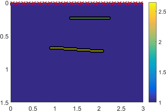
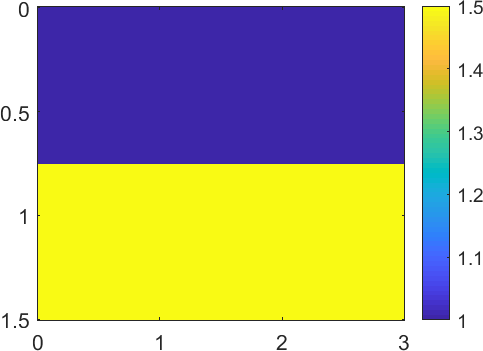
Fig. 1: Model acoustic impedance $\sigma({{\itbf x}})$ with two inclusions (left) and piecewise-constant velocity $c({{\itbf x}})$ (right). The crosses in the left plot indicate the sensor locations.The abscissa and ordinate are in km units. The colorbar displays the values of the impedance and velocity normalized by their constant values in the vicinity of the array.

Scattered field	True Born approximant
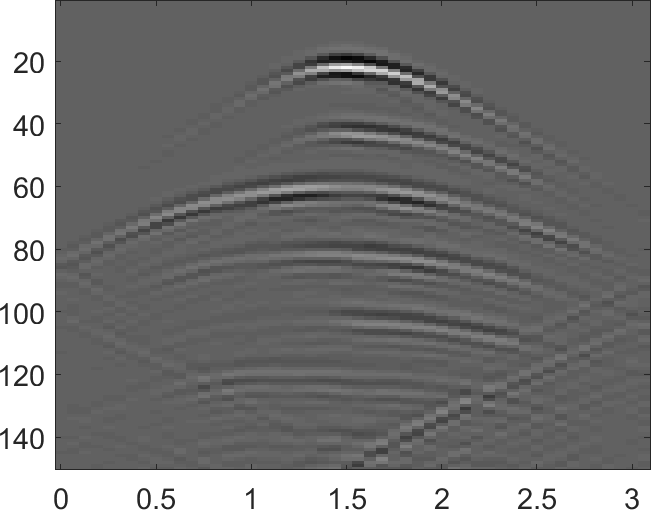
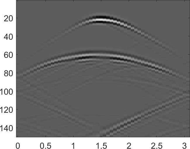
DtB for data with 10% noise	DtB for noiseless data

Fig. 2: The sound wave measured at the array (top left), true Born approximation (top right) and the outputs of Algorithm 6 for data with 10% noise (bottom left) and noiseless data (bottom right). The abscissa is the sensor location in $km$ units and the ordinate is the index $k$ of the discrete time instants $t_{k}=k\tau$, with $\tau=0.034s$. The plots are on the same gray scale.

Consider the 2D acoustic wave scattering problem in the medium shown in Fig. 1, where we plot the acoustic impedance $\sigma({{\itbf x}})$ and wave speed $c({{\itbf x}})$ normalized by their constant values at the array. The data ${\bf D}$ and its Born approximation ${\bf D}^{{\rm Born}}$ are obtained using finite-difference time-domain simulations with time step close to the CFL limit. The separation between the $m_{a}=50$ sensors and the time sampling rate $\tau$ are close to the Nyquist limit. The computational domain is the rectange shown in Fig. 1, with sides in km units. At the top boundary we have homogeneous Neumann conditions and at the remaining part of the boundary we have homogenenous Dirichlet conditions.

In the top left plot of Fig. 2 we display the raw scattered data due to the excitation from the sensor located in the middle of the array. The single scattering pattern (primaries) consist of two reflections from the two thin inclusions and the reflections from the domain boundary, as seen from the Born approximation displayed in the top right plot in Fig. 2. The other reflections in the top left plot are caused by multiple scattering between the inclusions and/or the boundary. The output of the Algorithm 6 is displayed in the bottom row of Fig. 2, for noiseless data in the right plot and data contaminated with 10% additive i.i.d. Gaussian noise in the left plot. Both results are almost the same as the true Born approximant.

6.2 2D elastic wave problem

The data ${\bf D}$ and the Born approximation ${\bf D}^{{\rm Born}}$ in this section are obtained by solving the elastic wave equation (136) with boundary conditions (139)–(140) and initial conditions (141) using a finite-difference time-domain method with time step satisfying the CFL condition for the shear wave. The spacing between the $m_{a}=25$ sensors in the array and the time sampling rate are close to the Nyquist limit for the shear wave. Therefore, the pressure wave is spatially oversampled. At each sensor location we consider both orientations of the external force source and measure both the horizontal and vertical velocities.

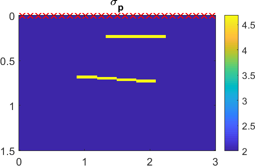
Fig. 3: The pressure wave impedance $\sigma_{p}({{\itbf x}})$ modeling two thin inclusions. The axes are in km units. Crosses indicate the sensor locations. The colorbar shows the impedance normalized by its value at the array.

Scattered field	True Born approximant	DtB output

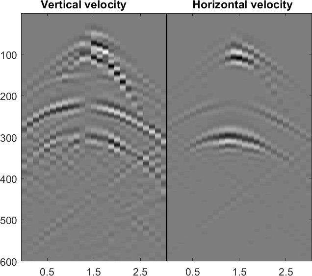
Fig. 4: The raw scattered field (left), the true Born approximant (middle) and the output of Algorithm 6 (right). The abscissa is the location of sensors in km units. These measure both the horizontal and vertical velocity components. The ordinate is the index $k$ of the discrete time instants $t_{k}=k\tau$, with $\tau=0.034s$. Because the horizontal response is stronger, we amplified the vertical response by the factor 8. This amplification highlights numerical artifacts in the vertical velocity plots. The plots are on the same gray scale.

In the first simulation we consider two thin inclusions embedded in a homogeneous background. The wave speeds $c_{p}$ and $c_{s}$ are constant, satisfying $c_{p}=2c_{s}$, so the shear wave impedance is $\sigma_{s}({{\itbf x}})=\sigma_{p}({{\itbf x}})/2$. In Fig. 3 we display the normalized (by the value of $\sigma_{s}({{\itbf x}})$ at the array) pressure wave impedance $\sigma_{p}({{\itbf x}})$.

We present results for the horizontal force exerted by the source located in the middle of the array. The left plot in Fig. 4 displays the raw array data, which contain the primary arrivals and the multiply scattered waves between the inclusions and/or the boundary of the domain. Since there are two waves traveling with different speeds, the primaries consist of two pressure waves and two shear waves reflected from the two inclusions and the domain boundaries. These can be seen in the middle plot in Fig. 4. Due to the excitation and the nearly layered medium, the dominant response is the horizontal velocity of the shear waves. The weaker vertical velocity response is amplified in the plots by the factor $8$, in order to display it on the same gray scale as the horizontal response. The output of the Algorithm 6 is shown in the right plot of Fig. 4. It is basically the same as the Born approximation, aside from some artifacts in the vertical velocity plot.

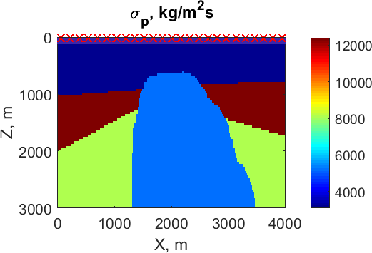
Fig. 5: Salt dome impedance model of the pressure wave impedance $\sigma_{p}({{\itbf x}})$. The abscissa and ordinate are in m units. The colorbar is in ${\rm kg}/({m}^{2}s)$ units. Crosses indicate the sensor locations.

Scattered field	True Born approximant	DtB output

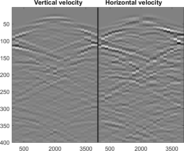
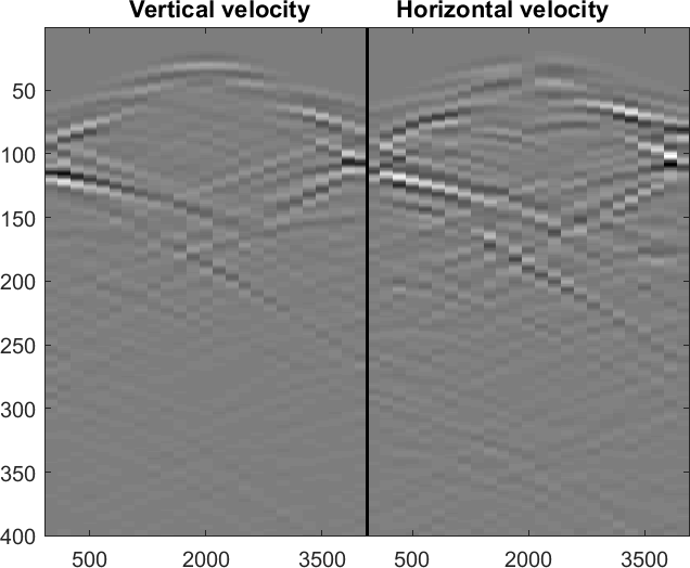
Fig. 6: Raw scattered field (left), the true Born approximant (middle) and the output of DtB transform (right). The abscissa is location of sensors measuring horizontal and vertical velocity components, and the ordinate is the index $k$ of the discrete time instants $t_{k}=k\tau$, $\tau=0.034s$. The plots are on the same gray scale.

The second simulation is motivated by the application of seismic exploration, and models a salt dome in a layered formation, as shown in Fig. 5. The pressure and shear wave speeds are constant and equal to 3100m/s and 1800m/s, respectively. The background pressure wave impedance is homogeneous and equal to 3100${\rm kg}/({\rm m}^{2}{\rm s})$. As in the first simulation, we consider both horizontal and vertical external forces and the data consist of both the horizontal and vertical velocities. In Fig. 6 we display the raw and processed data for the vertical force exerted from the source in the center of the array. In the left plot we show the raw data. Since the medium is far from layered, both responses are of the same order and there is no amplification factor in the plots. The primary reflections can be seen in the middle plot and the output of the Algorithm 6 is shown in the right plot. It matches the true Born approximation displayed in the middle plot in Fig. 6.

7 Summary

We introduced a robust algorithm for nonlinear processing of data gathered by an active array of sensors, which seeks to determine an unknown medium by probing it with pulses and measuring the resulting waves. These waves depend nonlinearly on the variations in the medium, modeled by an unknown reflectivity function. Many imaging methodologies ignore this nonlinearity and operate under the linear, single scattering (Born) assumption. This is adequate for a weak reflectivity. However, in strongly scattering media the nonlinear (multiple scattering) effects are significant and images based on the Born approximation have unwanted artifacts. The algorithm introduced in this paper seeks to map the array data gathered for an arbitrary (possibly large) reflectivity to the single scattering (Born) data, which can then be used by any linear imaging method. This mapping is called the Data-to-Born (DtB) transformation.

The algorithm is based on a data driven reduced order model which consists of a proxy wave propagator operator. The true wave propagator maps the wave from a given state at time $t$ to a future state at time $t+\tau$, where $\tau$ is the time sampling of the measurements. The proxy wave propagator is a projection of the true wave propagator on the space spanned by the snapshots of the wave field at the discrete times $t_{k}=k\tau$, for $k=0,\ldots,n-1$. It is constructed directly from the array data at $t_{k}=k\tau$, for $k=0,\ldots,2n-1$, with no knowledge of the reflectivity in the medium.

Our definition of the reflectivity function is based on the known fact that the main contribution to the Born approximation for a small array is due to variations of the logarithm of the impedance of the medium. The wave speed, which determines the kinematics (travel times) of the wave is assumed known. The DtB transformation is obtained using a factorization of the proxy wave propagator in two operators that have an approximately affine dependence on the reflectivity function. This allows the computation of the Fréchet derivative of the reflectivity to data mapping, which defines the Born approximation of the measurements.

The algorithm is developed for a generic hyperbolic system and we showed how it applies to the three types of linear waves: sound, electromagnetic and elastic. Because it consists of a sequence of algebraic operations that can be performed without knowing the exact wave propagation model, the algorithm is versatile and can be used as a black-box tool for any of these waves.

To ensure robustness for noisy data, we identified the unstable step in the algorithm and introduced a regularization procedure based on a spectral truncation of the data driven reduced order model. This regularization balances numerical stability and accuracy of data fitting, up to the order of the standard deviation of the noise. The performance of the algorithm is assessed with numerical simulations for both sound and elastic waves in two dimensions.

References

• [1] A. Abubakar, G. Pan, M. Li, L. Zhang, T. Habashy, and P. van den Berg, Three-dimensional seismic full-waveform inversion using the finite-difference contrast source inversion method, Geophysical Prospecting, 59 (2011), pp. 874–888.
• [2] J. Achenbach, Quantitative nondestructive evaluation, International Journal of Solids and Structures, 37 (2000), pp. 13–27.
• [3] K. Aki and P. Richards, Quantitative Seismology. Theory and Methods, 1980.
• [4] R. Alonso, L. Borcea, G. Papanicolaou, and C. Tsogka, Detection and imaging in strongly backscattering randomly layered media, Inverse Problems, 27 (2011), p. 025004.
• [5] A. C. Antoulas, D. C. Sorensen, and S. Gugercin, A survey of model reduction methods for large-scale systems, Contemporary mathematics, 280 (2001), pp. 193–220.
• [6] A. Aubry and A. Derode, Detection and imaging in a random medium: A matrix method to overcome multiple scattering and aberration, Journal of Applied Physics, 106 (2009), p. 044903.
• [7] M. I. Belishev, Recent progress in the boundary control method, Inverse Problems, 23 (2007), p. R1.
• [8] G. Beylkin, Imaging of discontinuities in the inverse scattering problem by inversion of a causal generalized radon transform, Journal of Mathematical Physics, 26 (1985), pp. 99–108.
• [9] G. Beylkin and R. Burridge, Linearized inverse scattering problems in acoustics and elasticity, Wave motion, 12 (1990), pp. 15–52.
• [10] B. Biondi, 3D seismic imaging, vol. 14, Society of Exploration Geophysicists Tulsa, 2006.
• [11] N. Bleistein, J. K. Cohen, W. John Jr, et al., Mathematics of multidimensional seismic imaging, migration, and inversion, vol. 13, Springer Science & Business Media, 2013.
• [12] L. Borcea, F. G. Del Cueto, G. Papanicolaou, and C. Tsogka, Filtering random layering effects in imaging, Multiscale Modeling & Simulation, 8 (2010), pp. 751–781.
• [13] L. Borcea, F. G. del Cueto, G. Papanicolaou, and C. Tsogka, Filtering deterministic layer effects in imaging, SIAM Review, 54 (2012), pp. 757–798.
• [14] L. Borcea, V. Druskin, and L. Knizhnerman, On the continuum limit of a discrete inverse spectral problem on optimal finite difference grids, Communications on Pure and Applied Mathematics, 58 (2005), pp. 1231–1279.
• [15] L. Borcea, V. Druskin, A. Mamonov, and M. Zaslavsky, Untangling the nonlinearity in inverse scattering with data-driven reduced order models, Inverse Problems, 34 (2018), p. 065008.
• [16] L. Borcea, V. Druskin, A. V. Mamonov, and M. Zaslavsky, A model reduction approach to numerical inversion for a parabolic partial differential equation, Inverse Problems, 30 (2014), p. 125011.
• [17] L. Borcea, V. Druskin, F. G. Vasquez, and A. Mamonov, Resistor network approaches to electrical impedance tomography, Inverse Problems and Applications: Inside Out II, Math. Sci. Res. Inst. Publ, 60 (2011), pp. 55–118.
• [18] L. Borcea, G. Papanicolaou, and C. Tsogka, Adaptive time-frequency detection and filtering for imaging in heavy clutter, SIAM Journal on Imaging Sciences, 4 (2011), pp. 827–849.
• [19]  , Time and direction of arrival detection and filtering for imaging in strongly scattering random media, Waves in Random and Complex Media, 27 (2017), pp. 664–689.
• [20] R. Brossier, S. Operto, and J. Virieux, Velocity model building from seismic reflection data by full-waveform inversion, Geophysical Prospecting, 63 (2015), pp. 354–367.
• [21] K. P. Bube and R. Burridge, The one-dimensional inverse problem of reflection seismology, SIAM review, 25 (1983), pp. 497–559.
• [22] C. Bunks, F. M. Saleck, S. Zaleski, and G. Chavent, Multiscale seismic waveform inversion, Geophysics, 60 (1995), pp. 1457–1473.
• [23] R. Burridge, The Gelfand-Levitan, the Marchenko, and the Gopinath-Sondhi integral equations of inverse scattering theory, regarded in the context of inverse impulse-response problems, Wave motion, 2 (1980), pp. 305–323.
• [24] Y. Chen, Inverse scattering via Heisenberg’s uncertainty principle, Inverse problems, 13 (1997), p. 253.
• [25] M. Cheney and B. Borden, Fundamentals of radar imaging, vol. 79, Siam, 2009.
• [26] J. F. Claerbout, Imaging the earth’s interior, vol. 1, Blackwell scientific publications Oxford, 1985.
• [27] M. Collins and W. Kuperman, Inverse problems in ocean acoustics, Inverse Problems, 10 (1994), p. 1023.
• [28] J. C. Curlander and R. N. McDonough, Synthetic aperture radar, vol. 396, John Wiley & Sons New York, NY, USA, 1991.
• [29] M. V. de Hoop, P. Kepley, and L. Oksanen, An exact redatuming procedure for the inverse boundary value problem for the wave equation, SIAM Journal on Applied Mathematics, 78 (2018), pp. 171–192.
• [30] V. Druskin and L. Knizhnerman, Gaussian spectral rules for the three-point second differences: I. a two-point positive definite problem in a semi-infinite domain, SIAM Journal on Numerical Analysis, 37 (1999), pp. 403–422.
• [31] V. Druskin, A. V. Mamonov, A. E. Thaler, and M. Zaslavsky, Direct, nonlinear inversion algorithm for hyperbolic problems via projection-based model reduction, SIAM Journal on Imaging Sciences, 9 (2016), pp. 684–747.
• [32] V. Druskin, A. V. Mamonov, and M. Zaslavsky, A nonlinear method for imaging with acoustic waves via reduced order model backprojection, SIAM Journal on Imaging Sciences, 11 (2018), pp. 164–196.
• [33] Y. M. Dyukarev, Indeterminacy criteria for the stieltjes matrix moment problem, Mathematical Notes, 75 (2004), pp. 66–82.
• [34] S. Fomel, E. Landa, and M. T. Taner, Poststack velocity analysis by separation and imaging of seismic diffractions, Geophysics, 72 (2007), pp. U89–U94.
• [35] K. Gallivan, E. Grimme, D. Sorensen, and P. Van Dooren, On some modifications of the Lanczos algorithm and the relation with Padé approximations, Mathematical Research, 87 (1996), pp. 87–116.
• [36] K. Gallivan, G. Grimme, and P. Van Dooren, A rational Lanczos algorithm for model reduction, Numerical Algorithms, 12 (1996), pp. 33–63.
• [37] I. M. Gel’fand and B. M. Levitan, On the determination of a differential equation from its spectral function, in Amer. Math. Soc. Transl., AMS, Providence, RI, 1955, pp. 253–304.
• [38] G. H. Golub and R. Underwood, The block Lanczos method for computing eigenvalues, in Mathematical software, Elsevier, 1977, pp. 361–377.
• [39] B. Gopinath and M. Sondhi, Inversion of the telegraph equation and the synthesis of nonuniform lines, Proceedings of the IEEE, 59 (1971), pp. 383–392.
• [40] R. G. Grimes, J. G. Lewis, and H. D. Simon, A shifted block Lanczos algorithm for solving sparse symmetric generalized eigenproblems, SIAM Journal on Matrix Analysis and Applications, 15 (1994), pp. 228–272.
• [41] S. Gugercin and A. C. Antoulas, A survey of model reduction by balanced truncation and some new results, International Journal of Control, 77 (2004), pp. 748–766.
• [42] T. M. Habashy, A generalized Gel’fand-Levitan-Marchenko integral equation, Inverse Problems, 7 (1991), p. 703.
• [43] G. Huang, R. Nammour, and W. Symes, Full-waveform inversion via source-receiver extension, Geophysics, 82 (2017), pp. R153–R171.
• [44] S. I. Kabanikhin and M. A. Shishlenin, Numerical algorithm for two-dimensional inverse acoustic problem based on Gel’fand–Levitan–Krein equation, Journal of Inverse and Ill-Posed Problems, 18 (2011), pp. 979–995.
• [45] I. Kac and M. Krein, On the spectral functions of the string, Amer. Math. Soc. Transl, 103 (1974), pp. 19–102.
• [46] M. G. Krein, Solution of the inverse Sturm-Liouville problem, in Dokl. Akad. Nauk SSSR, vol. 76 (1), 1951, pp. 21–24.
• [47]  , On the transfer function of a one-dimensional boundary problem of second order, in Dokl. Akad. Nauk SSSR, vol. 88, 1953, pp. 405–408.
• [48] A. E. Malcolm and M. V. de Hoop, A method for inverse scattering based on the generalized Bremmer coupling series, Inverse Problems, 21 (2005), p. 1137.
• [49] V. A. Marchenko, Some problems in the theory of one-dimensional second-order differential operators, Dokl. Akad. Nauk. SSSR, 2 (1950), pp. 457–560.
• [50] G. A. Meles, K. Wapenaar, and A. Curtis, Reconstructing the primary reflections in seismic data by Marchenko redatuming and convolutional interferometry, GEOPHYSICS, 81 (2016), pp. Q15–Q26.
• [51] S. Moskow, K. Kilgore, and J. C. Schotland, Inverse Born series for scalar waves, Journal of Computational Mathematics, 30 (2012), pp. 601–614.
• [52] F. Santosa, Numerical scheme for the inversion of acoustical impedance profile based on the Gelfand-Levitan method, Geophysical Journal International, 70 (1982), pp. 229–243.
• [53] P. Shen, W. W. Symes, C. C. Stolk, et al., Differential semblance velocity analysis by wave-equation migration, in 2003 SEG Annual Meeting, Society of Exploration Geophysicists, 2003.
• [54] C. C. Stolk and W. W. Symes, Smooth objective functionals for seismic velocity inversion, Inverse Problems, 19 (2002), p. 73.
• [55] W. Symes, Inverse boundary value problems and a theorem of Gel’fand and Levitan, Journal of Mathematical Analysis and Applications, 71 (1979), pp. 379–402.
• [56] T. L. Szabo, Diagnostic ultrasound imaging: inside out, Academic Press, 2004.
• [57] C. W. Therrien, Discrete random signals and statistical signal processing, Prentice Hall PTR, 1992.
• [58] G. Uhlmann, Travel time tomography, Journal of the Korean Mathematical Society, 38 (2001), pp. 711–722.
• [59] G. Uhlmann and A. Vasy, The inverse problem for the local geodesic ray transform, Inventiones mathematicae, 205 (2016), pp. 83–120.
• [60] J. Virieux and S. Operto, An overview of full-waveform inversion in exploration geophysics, Geophysics, 74 (2009), pp. WCC1–WCC26.
• [61] K. Wapenaar, F. Broggini, E. Slob, and R. Snieder, Three-dimensional single-sided Marchenko inverse scattering, data-driven focusing, Green?s function retrieval, and their mutual relations, Physical Review Letters, 110 (2013), p. 084301.
• [62] K. Wapenaar, J. Thorbecke, J. Van Der Neut, F. Broggini, E. Slob, and R. Snieder, Marchenko imaging, Geophysics, 79 (2014), pp. WA39–WA57.
• [63] A. B. Weglein, Multiple attenuation: an overview of recent advances and the road ahead, The Leading Edge, 18 (1999), pp. 40–44.