Abstract

We present a new application of the Regge-Teitelboim method for treating symmetries which are defined asymptotically. It may be regarded as complementary to the one in their original 1974 paper. The formulation is based on replacing an asymptotic plane by the two–sheeted “hourglass” shaped surface obtained by joining smoothly an incoming hyperboloid with an outgoing one. The hyperboloids have a fixed radius, and as one moves the center of the hourglass along the time axis one covers the whole of spacetime. The motivation is to study radiation, and the hourglass is well suited to the task because it is asymptotically null, and thus is able to register the details of the process. A simple parity condition for the fields on the hyperboloid is given. It specifies that as much radiation as is coming in as it is going out. With it, a Hamiltonian formulation of the symmetry of Bondi, van der Burg, Metzner and Sachs is developed fir both electromagnetism and gravitation. It is indispensable for the construction to have electric–magnetic duality asymptotically. For gravitation, a formulation for the linearized theory on the hourglass has not been explicitly constructed; but enough rudiments of it are given so that the main results can be established. A definition for angular momentum wish is conserved (for which the “magnetic sector” is essential) is given. It incorporates an interrelationship between spin and charge. For the gravitational field, Taub-NUT space appears as the analog of a magnetic pole.

Regge-Teitelboim analysis of the symmetries of electromagnetic and gravitational fields on asymptotically null spacelike surfaces C. Bunster, A. Gomberoff, A. Perez

Chapter 0 Regge-Teitelboim analysis of the symmetries of electromagnetic and gravitational fields on asymptotically null spacelike surfaces

To Tullio, for old times’ sake

1 Introduction

The 1974 paper by Regge and Teitelboim [1] contained two main results: (i) A completion of Dirac’s analysis [2] of the role of constraints in field dynamics that was necessary in order to account for the different character of the gauge transformations which do not change the physical state (“proper gauge transformations”), from those which do (“improper gauge transformations”). It was found that, in the latter case, Dirac’s “weakly vanishing” generators have to be improved by the addition of a surface integral and do not vanish weakly. The surface integral gives the value of the charge associated to the improper transformations. (ii) An application of (i) to obtain a Poincaré invariant formulation of the theory of gravitation on spacelike surfaces which are asymptotically planes.

We develop below a new application of the method which is based on replacing an asymptotic plane by the two–sheeted “hourglass” shaped surface obtained by joining smoothly an incoming hyperboloid with an outgoing one. The hyperboloids have a fixed radius, and as one moves the center of the hourglass along the time axis one covers the whole of spacetime. The motivation is to study radiation, and the hourglass is well suited to the task because it is asymptotically null, and thus is able to register the details of the process. In contradistinction, if one goes far enough on an asymptotic plane, the radiation emitted by a confined source has not enough time to reach there.

A simple parity boundary condition, with a direct physical meaning, for the fields defined on the hourglass is given. With it, a Hamiltonian formulation of the symmetry of Bondi, van der Burg, Metzner and Sachs [3; 4; 5] is developed. The formulation yields a Hamiltonian definition of the Bondi “news”. For electromagnetism, an interrelationship between spin and the BMS charge is brought out, and manifest electric-magnetic duality is achieved by introducing a second vector potential. For the gravitational field, Taub-NUT space appears as a gravitational magnetic pole and the magnetic BMS charges are exhibited. However, and expression for their conjugates, the magnetic supertranslations, is lacking.

The “hourglass” construction, the parity conditions on it and the intimate connection between BMS invariance and electric–magnetic duality were reported in [6]

If one gives initial data on one hyperbolic hourglass, the Hamiltonian equations of motion determine the canonical variables on any other hyperbolic hourglass. However, the initial data should only be specified on one half of the hourglass. This is because a point, which is not at infinity, lying, say, on the outgoing half of one hourglass at a given time also lies on the incoming half of another hourglass at a later time. This double counting does not happen at infinity, and hence one needs to specify the radiation on the other half. That is, if one is giving the data on the outgoing half one must specify in addition the incoming Bondi news. But the parity condition states that they are equal to the outgoing ones, and therefore it is sufficient to specify just the data on the outgoing half of the hourglass (or, viceversa, on the incoming one). In this sense the hyperbolic hourglass is a Cauchy surface.

If compared with an hourglass formed by incoming and outgoing light cones, the one formed by hyperboloids has the advantage of being spacelike and therefore permitting direct step by step use of the Dirac’s procedure with the Regge-Teitelboim complement, which has been battle-tested, and in which all the structures that appear (action, Hamiltonian, Poisson and Dirac brackets, surface deformations, most general permissible motion) are well, and tightly, defined from the start.

Furthermore, the slicing by hyperbolic hourglasses of fixed radius and varying center has the essential property of covering the whole of spacetime, in contradistinction with the foliations by hyperboloids of fixed center and varying radius, used previously by many authors, which only cover part of it.

The structure of the paper is the following. In order to make the treatment self-contained and set the notation and terminology, section 2 begins by reviewing the general procedure. Section 3 discusses the foliation by hyperbolic hourglasses of the same radius and different center. Next, section 4 contains an analysis of the asymptotic properties of the free electromagnetic field on the hyperbolic hourglass foliation. The discussion is given in detail, because practically all the results derived for electromagnetism can be translated literally to the gravitational case, whose treatment becomes then considerably lighter. Section 5 is then devoted to the gravitational case.

Three appendices are included: appendix A gives explicit expressions for the Poincaré generators on the hyperbolic hourglass foliation. Appendix B gives the details of the preservation in time of the parity boundary conditions. Appendix C provides a “dictionary” for translating in the gravitational case the variables which appear in the present Hamiltonian treatment with those employed in the original BMS light cone analysis.

2 Hamiltonian field dynamics, surface deformations, gauge transformations, surface integrals, and conservation laws.

1 Quick review of formulation.

In the formulation of field dynamics in which the state is defined on a general spacelike surface developed by Dirac [2], and completed by Regge and Teitelboim [1] to incorporate symmetries which are defined asymptotically, the generator–through Poisson brackets–of the “most general permissible motion” has the form

$$H[\xi;\lambda]=H_{0}[\xi;\lambda]+Q[\xi;\lambda]\,,$$ (1)

where $H_{0}[\xi;\lambda]$ is an integral over the spacelike surface on which the state is defined, of the form

$$H_{0}[\xi;\lambda]=\int d^{3}x\left(\xi^{\mu}{\mathcal{H}}_{\mu}+\lambda^{a}G_{a}\right)\,,$$ (2)

and $Q[\xi,\lambda]$ is a surface integral over the asymptotic boundary of that spacelike surface.

The surface integral $Q[\xi;\lambda]$ is included to make well defined the functional derivatives of $H[\xi;\lambda]$, so that one has,

$$\delta H[\xi;\lambda]=\int d^{3}x\left(\frac{\delta H}{\delta\phi}\delta\phi+\frac{\delta H}{\delta{\pi}}\delta\pi\right)\,,$$ (3)

without any surface terms. This means that the contribution of the asymptotic part of the field is already included in (3). Here we have abbreviated as $(\phi,\pi)$ all the canonical field variables of the theory.

In (2) the ${\mathcal{H}}_{\mu}$ are the generators of deformations of the spacelike surface in which the state is defined, while the $G_{a}$ are the generators of internal gauge transformations. They are both constrained to vanish, that is, they are weakly equal to zero:

$${\mathcal{H}}_{\mu}\approx 0,\ \ G_{a}\approx 0\,.$$ (4)

Proper and improper gauge transformations

If the parameters $(\xi,\lambda)$ are such that the surface integral $Q[\xi;\lambda]$ vanishes, the motion generated by $H_{0}[\xi;\lambda]$ is called a “proper” gauge transformation [7], and it it is not a symmetry, but rather an expression of the fact that the system is described by variables which are redundant. This normally happens when they vanish at infinity, but there are important cases, in both electromagnetism and gravity [1] where the surface integrals vanish even though the parameters do not vanish at infinity but obey parity conditions there. In that case the transformation is still proper. For an internal symmetry one feels on safe grounds stating that a proper gauge transformation does not change the physical state on a given spacelike surface. For the case of a surface deformation this point of view may be kept for purely tangential deformations (changes of spatial coordinates), but if the deformation has a normal component the hypersurface is geometrically deformed, and therefore, if one can “perform local observations inside”, one would expect the physical state to change. On the other hand if one only performs observations at infinity, then one may safely take the point of view that proper normal deformations are also gauge transformations, and do not change the physical state either. If $(\xi,\lambda)$ are such that the surface integral $Q[\xi;\lambda]$ does not vanish the motion is called an “improper” gauge transformation, and one expects it to change the physical state. As a consequence of (3), the functional form of the transformation generated by (1) is the same if the transformation is proper or improper, the difference is only introduced by the asymptotic behavior of the transformation parameters.

The difference between proper and improper transformations manifests itself at the level of the action principle in which (1) is the Hamiltonian, in the fact that the constraints (4) are obtained from it by extremizing the action with respect to $\xi$ and $\lambda$ keeping fixed the part that contributes to the surface integral $Q[\xi,\lambda]$. Thus, (4) states that the generator of proper gauge transformations vanishes weakly. On the other hand, for improper gauge transformations this does not happen:

$$H[\xi;\lambda]\approx Q[\xi;\lambda]\neq 0\,.$$

If one is interested in the action of an asymptotic motion, one gives the asymptotic part of the transformation and continues it inside in an arbitrary manner. The way in which one chooses to continue inside is irrelevant because any two continuations differ by a proper gauge transformation. It is however necessary to continue, because it is only the sum of the volume part of the generator and the surface term which has well defined functional derivatives and is therefore capable of acting through a Poisson bracket. Neither the volume part alone, nor the surface integral alone has that capability. Alternatively, one may choose a particular continuation inside by fixing the gauge. If this is done, the combined set of the original gauge constraints and the gauge conditions become second class, and one can pass from the original Poisson bracket to the associated Dirac bracket, in terms of which the second class constrains vanish strongly and have zero bracket with everything. Then the surface term stands alone and is capable to act as itself as a generator through the Dirac bracket.

Commutation of deformations

The constraint–generators ${\mathcal{H}}_{\mu}$, $G_{a}$ are first class. If we denote collectively by $\Lambda_{1}=(\xi_{1},\lambda_{1})$, $\Lambda_{2}=(\xi_{2},\lambda_{2})$, the parameters of any two motions one has, for proper gauge transformations,

$$\Big{[}H[\Lambda_{1}],H[\Lambda_{2}]\Big{]}=H[\Lambda_{12}]\,,$$ (5)

where the commutator $\Lambda_{12}=-\Lambda_{21}$ of the two original infinitesimal transformations is a bilinear expression of $\Lambda_{1}$, $\Lambda_{2}$ and their derivatives (in practice, first derivatives, with coefficients which in general depend on the fields). For improper transformations it may happen that Eq. (5) is relaxed by the appearance of a central extension on its right hand side, that is, by the addition to $H[\Lambda_{12}]$ of a term that has zero Poisson brackets with all the dynamical variables. This is not allowed for proper transformations because it would spoil the first class character of the constraints; i.e. the vanishing of the constraints would not be preserved by the transformation. This obstruction to the presence of a central extension does not happen for improper transformations because the charge $Q$ is not constrained to be zero.

Given any theory one may calculate $\Lambda_{12}$ by working out directly the Poisson bracket on the left side of (5). However, if one has geometrical insight on the nature of the motions at hand one may write down the result without doing that calculation. For example, for a Yang-Mills theory, with structure constants $C_{\ bc}^{a}$, one has

$$\lambda_{12}^{c}=C_{\ ab}^{c}\lambda_{1}^{a}\lambda_{2}^{b}\ ,$$

and for two surface deformations within an arbitrary Riemannian spacetime with Lorentzian signature one has [8; 9],

$$\xi_{12}^{\perp} = \xi_{1}^{i}\xi_{2,i}^{\perp}-\xi_{2}^{i}\xi_{1,i}^{\perp}\,,$$ (6)

$$\xi_{12}^{i} = g^{ij}\left(\xi_{1}^{\perp}\xi_{2,j}-\xi_{2}^{\perp}\xi_{1,j}\right)+\xi_{1}^{j}\xi_{2,j}^{i}-\xi_{2}^{j}\xi_{1,j}^{i}\,,$$ (7)

where $g_{ij}$ is the metric of the spacelike surface.

No royal road

Lastly, we elaborate on the sentence “…The surface integral $Q[\xi;\lambda]$ is included in (1) to make well defined the functional derivatives of $H[\xi;\lambda]$…” written above. To achieve this it is necessary to find an appropriate set of boundary conditions. There is no foolproof, inductive method for that. One rather works by trial and error and there is no guarantee of success. The procedure in practice is as follows: (i) A tentative set of asymptotic conditions is obtained by applying the asymptotic transformations that one wants to have present, to a simple field configuration that one also wants to have present. For example, in the case of gravitation, one would boost a Schwarzschild field; or, in electromagnetism, a Coulomb field. (ii) One extracts properties of the result obtained that can be formulated independently of the specific original configuration, and uses them as a starting ansatz. For example, one may retain a decay rate in inverse powers of the radial distance and a parity condition for the coefficients.(iii) One finds the most general parameters $(\xi,\lambda)$ which preserve the ansatz. It may happen then that that set of parameters does not contain all the symmetries that one was interested in (for example, the complete Poincaré group). Then one relaxes the ansatz to make room. If success is achieved – meaning, in the example just given, that one has the Poincaré group or more – one checks whether the surface integral that appears in the variation of the $H_{0}$ is the variation of a finite surface integral, or, as one says colloquially, “if the $\delta$ can be taken out”. If this happens one is done. If it does not, one modifies the boundary conditions in the light of the nature of the failure. With luck and dedication the process converges and one finally succeeds.

3 Foliation of Minkowski space by hyperboloids of the same radius and different centers

1 Incoming and outgoing hyperboloids

In Minkowski space it is natural to define the state on a three-dimensional spacelike hyperboloid, because that surface is mapped onto itself by a Lorentz transformation. In this sense, hyperboloids are more adequate to the special principle of relativity than the planes corresponding to inertial frames, for which the boosts are interchanged with spatial translations. This possibility was considered by Dirac in 1940 [10] and he called it the “point form of field dynamics” with the term “point” referring to the center of the hyperboloid.

A spacelike hyperboloid with center at $x_{(0)}^{\mu}$ and radius $\tau_{0}$ obeys the equation

$$(x^{\mu}-x_{(0)}^{\mu})(x_{\mu}-x_{(0)\mu})=-\tau_{0}^{2}\,.$$ (8)

Actually, Eq. (8) describes two disjoint hyperboloids, one with $x^{0}>x_{(0)}^{0}$ (“outgoing hyperboloid”) and another with $x^{0}<x_{(0)}^{0}$ (“incoming hyperboloid”). Although Dirac did not discuss foliations of spacetime by means of a family of hyperboloids, this has been done by many authors but to our knowledge in all cases treated so far the foliation has been defined by keeping $x_{(0)}^{\mu}$ fixed and letting $\tau_{0}$ vary as one passes from one hyperboloid to the next.

In other words, the foliations used previously have consisted of a sequence of hyperboloids with fixed center and varying radius. These foliations have the advantage that the four $x^{\mu}$ are treated on the same footing so Lorentz invariance is manifest; but the price payed is extremely high, because only a small part of Minkowski space is covered, and moreover, a spurious explicit dependence on the varying $\tau_{0}$, which is taken as the time $\tau$, is introduced. Here we take the other natural option, we keep the radius $\tau_{0}$ fixed and we allow the position of the center to vary. This is a direct extension of what is done with null foliations, which may be regarded as being the limit $\tau_{0}\rightarrow 0$. The actual value of $\tau_{0}$ will turn out to be irrelevant, since all the quantities of physical interest will incorporate naturally $\tau_{0}$ in their units.

2 The hyperbolic hourglass

The hyperbolic hourglass consists of an outgoing hyperboloid with center $x^{\mu}_{(0)}=(-\tau_{0},0)$ joint to an incoming one with center $x^{\mu}_{(0)}=(\tau_{0},0)$. At time $t$ it has spatial coordinates $(r,\vartheta,\varphi)$, whose range is:

$$-\infty< r <+\infty,$$

$$0\leq \vartheta \leq\pi,$$

$$0\leq \varphi <2\pi.$$

It is defined parametrically from Minkowskian coordinates $(x^{0},\vec{x})$ through

$$x^{0} = t+r\sqrt{1+\frac{\tau_{0}^{2}}{r^{2}}}+\tau_{0}\ \ \ r\leq 0$$ (9)

$$x^{0} = t+r\sqrt{1+\frac{\tau_{0}^{2}}{r^{2}}}-\tau_{0}\ \ \ r\geq 0,$$ (10)

and

$$\vec{x}=r\hat{r}\ ,\ \ -\infty<r<+\infty,$$ (11)

where the unit vector $\hat{r}$ is given by

$$\hat{r}=(\cos\vartheta\cos\varphi,\cos\vartheta\sin\varphi,\sin\vartheta).$$ (12)

The radius $\tau_{0}$ is taken to be positive. The embedding defined by the above equations is continuously differentiable. The tangent vectors are continuous at $r=0$ and the surface has a well defined global orientation.

The hyperbolic hourglass may be regarded as a spacelike deformation of the full (pass and future) lightcone, with an orientation inherited from the propagation of a light front that comes in, goes through itself, and then comes out. Since this wave propagation process is physically smooth, fields defined on the global coordinate system just described should be smooth. (The parametric equations (9)-(11) automatically incorporate the antipodal map [15] [16], which amounts to rewriting them by using a positive $r$ for both sheets of the hyperboloid and inverting the orientation of the two-spehere at a given $r$. That is, keeping (9)-(11) for $r\geq 0$ and setting, $r^{\prime}=-r$, $\hat{r}^{\prime}=-\hat{r}$, for $r\leq 0$.)

If one considers an incoming wave which is not spherically symmetric, then the spacetime point at which the wavefront goes through itself will be different for different $\hat{r}$’s. But in the present paper we are only interested in the analysis of the asymptotic region and therefore the details of what happens inside are irrelevant. The key aspects are the asymptotic hyperbolic shape and its orientation inherited from that of an incoming wave that goes through itself and becomes outgoing.

Figure 1 shows the embedding in Minkowski space of a single hyperbolic hourglass, figure 2 exhibits the slicing of Minkowski space by a one parameter family of hyperbolic hourglasses and figure 3 shows a sequence of Penrose diagrams with hyperbolic slicings of different radius $\tau_{0}$.

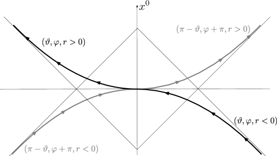
Figure 1: The hyperbolic hourglass. The figure shows a two dimensional cut of an incoming hyperboloid and an outgoing one which are joint smoothly at at $r=0$. The arrows show the direction of increasing $r$, which coincide asymptotically with the direction of propagation of a wave that comes in, goes through itself, and then comes out. If the incoming wave is not spherically symmetric, the spacetime point at which the wavefront goes through itself will be different for different $(\vartheta,\varphi)$. For the analysis of the asymptotic region the details of what happens inside are irrelevant. The key aspects are the asymptotic hyperbolic shape and its orientation inherited from that of an incoming wave that goes through itself and becomes outgoing.

Figure 2: Slicing by hyperbolic hourglasses. A given spacetime point is labeled by two set of coordinates. In the case of the point $P$ shown in the figure, these are $(t=0,r,\vartheta,\varphi)$ and $(t=3\tau_{0},-r,\pi-\vartheta,\varphi+\pi)$.

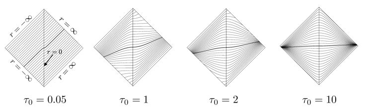
Figure 3: Limits $\tau_{0}\rightarrow 0$ and $\tau_{0}\rightarrow\infty$ for Minkowski space. The succession of conformal diagrams shows from left to right how the surfaces of the hourglass foliation are deformed from nearly light cones to nearly planes as $\tau_{0}$ increases from a very small value to a very large one. To better illustrate the effect, different members of the foliation are shown in the different figures of the sequence; but, to keep track of the deformation, the surface at $t=0$ (shown with a heavy line) in all cases. The Penrose diagram has been doubled to admit negative values of $r$ in the left triangular area. This doubling shows how the curves of constant $t,\vartheta,\varphi$ are smooth spacelike curves that connect asymptotically past and future null infinities. The scale of the lenght $\tau_{0}$ is irrelevant for the effect described in the figure, which only depends on the ratios between the different $\tau_{0}$’s shown.

4 Electromagnetic field in Minkowski space

We will analyze in this section the case of the electromagnetic field on a fixed Minkowskian background. Practically all the features that will be encountered in the gravitational case already appear in this technically simpler context.

The main difference which does not hinder the analogy is that, since the background is fixed, its Poincaré symmetry appears as a global symmetry rather than an asymptotic gauge symmetry. There are no constraints associated with the surface deformation $\xi$, which are not varied in the action principle. The ${\mathcal{H}}_{\mu}$ in (2) are replaced by the energy and momentum densities of the electromagnetic field

$${\mathcal{H}}_{\perp}^{(elm)} = \frac{1}{2}\left(g^{-\frac{1}{2}}\pi_{i}\pi^{i}+\frac{1}{2}g^{\frac{1}{2}}F^{ij}F_{ij}\right)\,,$$ (13)

$${\mathcal{H}}_{i}^{(elm)} = F_{ij}\pi^{j}\,.$$ (14)

The only gauge symmetry present in the problem is the electromagnetic one, whose generator is

$${\cal G}=-\pi_{,i}^{i}\approx 0\,.$$ (15)

Here $A_{i}$ is the vector potential, $\pi^{i}$ its conjugate momentum, and $g_{ij}$ is the metric on the hourglass, and $g$ denotes its determinant.

If instead of having a fixed background we were considering dynamically coupled electromagnetic and gravitational fields, then expressions (13), (14) would be added to their gravitational counterparts discussed in section 5, and the sum would be constrained to vanish. The asymptotic analysis given below would still hold because at large distances the spacetime would be flat. Then the asymptotic symmetry transformations of the coupled Einstein-Maxwell system would be those discussed here (internal electromagnetic, and Poincaré transformations) and the additional gravitational supertranslations.

We will now discuss the Poincaré and proper and improper gauge transformations for the electromagnetic field on the hourglass slicing. In this case the time equal constant surface is left invariant under the Lorentz group, whereas it is mapped onto a different hyperboloid by spacetime translations. Thus if one compares the situation with $t=$ constant planes, one sees that the roles of spatial translations and boosts are interchanged.

1 Asymptotic boundary conditions

Power expansion near $r=\pm\infty$

By applying the procedure described at the end of Sec. 2, starting from the Coulomb field written in hyperbolic coordinates, one is led to the boundary conditions,

$$A_{a} = a_{a}^{(0)}+a_{a}^{(1)}r^{-1}+\mathcal{O}(r^{-2})\,,$$ (16)

$$A_{r} = a_{r}^{(2)}r^{-2}+\mathcal{O}(r^{-3})\ ,$$ (17)

$$\pi^{a} = \pi_{(2)}^{a}r^{-2}+\mathcal{O}(r^{-3})\,,$$ (18)

$$\pi^{r} = \pi^{r}_{(0)}+\mathcal{O}(r^{-1})\,,\ \ \ \ \ \ \ \$$ (19)

$$\lambda = \lambda_{(0)}+\mathcal{O}(r^{-1}),$$ (20)

Here $\lambda$ is the Lagrange multiplier that accompanies the gauge generator (15). In addition to the power law decays (16)–(20) it is necessary to introduce parity conditions. This is achieved by splitting some of the variables in longitudinal and transverse parts as follows

$$a^{(0)}_{a}=\nabla_{a}F+\star\nabla_{a}\bar{G}\,,$$ (21)

$$h_{a}=\gamma^{\frac{1}{2}}\left(\nabla_{a}N+\star\nabla_{a}\bar{N}\right)\,.$$ (22)

Here,

$$\star\nabla_{a}=\gamma^{\frac{1}{2}}\epsilon_{ab}\nabla^{b}\,,$$ (23)

where $\gamma$ is the determinant of the metric $\gamma_{ab}$ on the unit two-sphere. The “news” vector $h^{a}$ in (22), which will play a central role in what follows, is defined by

$$h^{a}=\frac{1}{\tau_{0}^{2}}\left(\pi^{a}_{(2)}+\gamma^{\frac{1}{2}}\gamma^{ab}f_{br}^{(2)}\right)\,,$$ (24)

for $r\rightarrow\pm\infty$, where the $f^{(2)}_{br}$ is the leading order coefficient of $F_{br}$. In Minkowski coordinates the news correspond to an electromagnetic field that decays as $r^{-1}$, that is to a wave emerging from a confined source $(r\rightarrow+\infty)$, or converging towards an absorber$(r\rightarrow-\infty)$. For an accelerating electric charge $e$ one has from the Lienard-Wiechert field,

$$\gamma^{\frac{1}{2}}f^{ar}_{(2)}\vec{\partial}_{a}=\pi_{\left(2\right)}^{a}\vec{\partial}_{a}=-2e\gamma^{\frac{1}{2}}\hat{r}\times\left(\hat{r}\times\vec{a}\right),$$

where $\vec{a}$ is the acceleration in rest frame of the emitter (outgoing wave) or absorber (incoming wave). See for example, [17; 18].

On the entire hourglass this field stems from

$$F_{rad}=F_{ret}-F_{adv}$$

introduced by Dirac[19], which is derived from the function,

$$\frac{1}{r}\delta(t-r),\ \ \ \ \ -\infty<r<\infty\ .$$

This function is not a Green function, but a solution of the homogeneous equation: the difference $F_{ret}-F_{adv}$. Therefore it has as much radiation coming in as going out, and obeys the parity conditions that will be discussed next.

Parity conditions

The parity conditions will be then the following,

$$\left.(F,\lambda_{(0)},N,\bar{N})\right|_{+\infty}=\left.(F,\lambda_{(0)},N,\bar{N})\right|_{-\infty}\ \ \mbox{for each }(\vartheta,\varphi).$$ (25)

Parity conditions play a fundamental role in the Regge-Teitelboim discussion of Poincaré invariance on asymptotic planes. We see that when dealing with Bondi, Metzner, Sachs invariance on hyperboloids, they again come in. The reason for their appearance is discussed next.

Surface deformation algebra

The surface deformations involved in the present analysis are Poincaré deformations of the hypersurface, which are motions generated by the Killing vectors given in appendix A, and besides them, gauge transformations. If one evaluates the commutator of any two such deformations one finds the following results for the asymptotic part of the commutator:

(i) Two Poincaré deformations close according to the Poincaré group.

(ii) Spacetime translations commute with improper gauge transformations.

(iii) The commutator of a Lorentz transformation with Killing vector $\xi_{\text{Lorentz}}$ and an improper gauge transformation with parameter $\lambda(\vartheta,\varphi)$ at infinity, is a gauge transformation with parameter,

$$\zeta=\xi_{\text{Lorentz}}^{a}\partial_{a}\lambda.$$ (26)

The results (i)–(iii) are the expressions, in terms of deformations, of the electromagnetic BMS algebra.

Equation (26), which technically stand from the fact that the Lorentz group acts asymptotically as a Lie derivative on the two sphere (appendix A) has a profound consequence: it mixes improper gauge transformations with spacetime motions. This provides a tantalizing confirmation of the fact that improper gauge transformations are physically relevant motions that cannot be “factored away”.

2 The hyperbolic hourglass as an unconventional Cauchy surface

The physical motivation for the parity conditions is very simple. They essentially state that for a closed system (the free electromagnetic field in this case) everything that comes in must come out. That is, one allows for non–vanishing incoming and outgoing fluxes of energy, momentum, and other (BMS) charges; but requires that the net flux should be equal to zero.

This requirement, which physically is a condition connecting the remote past with the remote future, can be formulated as a fixed time statement, because the spacelike hyperbolic hourglass is asymptotically tangent to the past and future lightcones. This is the reason for bringing in the hourglass in the first place.

When regarded as an initial value surface, the hourglass has the unconventional feature, that a point, which is not at infinity, lying, say, on the outgoing half of one hourglass at a given time, also lies on the incoming half of another hourglass at a later time. This implies that one cannot give freely initial value data on the complete hourglass but only on half of it, the outgoing half for example. However, the double counting of points does not happen at infinity, so if one gives data on the outgoing half one should specify additionally the incoming radiation, that is one should give the news at $r=-\infty$. But this is precisely what the parity condition does, stating that the incoming news are equal to the outgoing ones. Thus it is sufficient to specify just the data on the outgoing half of the hourglass (or, viceversa, on the incoming one) if the parity condition is imposed.

Therefore one must bring in the complete hourglass in order to deal in Hamiltonian terms with the interrelationship between past and future, but one only gives initial value data on one half of it, together with asymptotic information on the other half. In this sense the hourglass is a Cauchy surface.

3 Poincaré invariance of the boundary conditions. Fiber memory

One must demand, by consistency, that the boundary conditions (16)–(20) and the parity conditions (25) should be preserved under the Poincaré group. This can be efficiently analyzed by writing the equations of motion in Hamiltonian form,

$$\dot{A}_{i} = -F_{ij}\xi^{j}+g^{-1/2}\xi^{\perp}\pi_{i}+\partial_{i}\lambda\,,$$ (27)

$$\dot{\pi}^{i} = (\pi^{i}\xi^{j})_{,j}-\pi^{j}\xi_{,j}^{i}+(\xi^{\perp}F^{ji}g^{1/2})_{,j}\ ,$$ (28)

and taking as the deformation parameters that multiply the generators (13), (14) to be the components, $\xi^{\perp}$ and $\xi^{i}$ of the Poincaré Killing vectors given in appendix A.

The preservation of the boundary conditions (16)–(20) is straightforward. One first verifies Lorentz invariance which is simpler because the hyperbolic hourglass is Lorentz invariant. With this established, it is sufficient to check invariance under time translations, which is more laborious but straightforward.

Next one turns to the conditions (25). The preservation of the parity conditions under Lorentz transformations is evident because they map each asymptotic region into itself. One needs then only be concerned with time translations. Under them, the equation of motion for the leading order term of $A_{a}$ is,

$$\dot{a}_{a}^{0}=\gamma^{-\frac{1}{2}}h_{a},$$ (29)

for $r\rightarrow\pm\infty$. Its longitudinal component is

$$\dot{F}=N,$$ (30)

which shows that the preservation in time of the parity of $F$ is automatically satisfied because of the parity conditions on $N$. The parity of $F$ is also preserved under improper gauge transformations because of the parity condition on $\lambda_{(0)}$. For $\lambda_{(0)}$ itself there is nothing to check because it has no equation of motion.

The preservation of the parity conditions for $N$ and $\bar{N}$ pose no problem either, as it is shown in appendix B.

Equation (30) has a highly non trivial content. It shows that, even when the generator of improper gauge transformations does not act, i.e., when $\lambda_{(0)}=0$, and one is only moving in the time $t$, there is still a displacement,

$$\delta F=N\delta t$$ (31)

along the U(1) fiber of amount $N\delta t$ when a time $\delta t$ elapses. That is: (i) If there are no news (and one does not change the gauge frame) $F$ is conserved, (ii) If there are news during a time interval the value of $F$ changes from $F_{\mbox{\tiny before}}$ to $F_{\mbox{\tiny after}}$ according to the integral of (30) over the time interval. That is, $F$ “remembers” the news, and for that reason is called the “fiber memory”. Another kind of memory, “charge memory” will be encountered below in section 9.

It is important to realize that (31) is not just a “redefinition of $\lambda_{(0)}$ by the amount $N$”. This is because $\lambda_{(0)}$ is not in the phase space, and can be held fixed in the variation of the Hamiltonian, whereas $N$ is a dynamical variable, which obeys a (gauge invariant) equation of motion and hence cannot be held fixed.

4 BMS charges

Electric BMS charge

Taking into account the parity condition on $\lambda_{(0)}$ one finds that the surface integral that must be added to the electromagnetic gauge generator to include improper transformations is given by

$$\oint\lambda_{(0)}Q$$ (32)

where the gauge charge $Q$ is given by

$$Q\left(\vartheta,\varphi\right)=\left.\pi_{(0)}^{r}\right|_{+\infty}-\left.\pi_{(0)}^{r}\right|_{-\infty}\equiv Q_{+}+Q_{-}.$$ (33)

It is important to interpret this expression appropriately. The hourglass is a construct that enables one to keep track, within the Hamiltonian formalism, of the incoming and outgoing radiation in an economic manner, that is without introducing separate overlapping incoming and outgoing hyperbolic patches. This brings in a redundancy: one way or another space its counted twice. We just saw one instance of this above in connection with the initial value data. The redundancy strikes again in expression (33) for the charge. If one considers the Coulomb field of a particle of charge $e$ at rest at $x^{i}=0$ one finds,

$$Q_{+}\left(\vartheta,\varphi\right)=\frac{e}{4\pi}\sin\vartheta$$

and

$$Q_{-}\left(\vartheta,\varphi\right)=\frac{e}{4\pi}\sin\vartheta$$

and hence

$$Q\left(\vartheta,\varphi\right)=2\frac{e}{4\pi}\sin\vartheta$$ (34)

The factor two arises because one is counting twice: $Q_{+}$ is the charge as seen in the outgoing description of space, while $Q_{-}$ is the same charge as seen from its incoming replica. This point will reappear below in connection with radiation rates.

Magnetic BMS charge

There is a magnetic analog of (33) given by

$$\bar{Q}=\left.\epsilon^{ab}\nabla_{a}a^{(0)}_{b}\right|^{+\infty}_{-\infty}=\left.\gamma^{1/2}\nabla^{2}\bar{G}\right|^{+\infty}_{-\infty},$$ (35)

which is conserved as a consequence of (29) and the parity condition for $\bar{N}$,

$$\dot{\bar{Q}}=0,$$ (36)

In the electric representation this conservation law appears as an “accidental”, because it does not follow from a symmetry of the action. The formalism becomes complete if one introduces a second potential, so that the electric and magnetic charges are treated on the same footing. This completion of the formalism may be regarded as a matter of elegance and economy, but not of necessity, for questions that can be asked within the electric representation. But, as we will see further below, it becomes essential when one discusses Lorentz transformations. Therefore we recall it right away.

5 Asymptotic two potential formulation

One brings in a new, “magnetic” vector potential $\bar{A}$. For the present purposes it is sufficient to do so only asymptotically. The potential $\bar{A}$ satisfies,

$$\pi^{r}=-\epsilon^{ab}\partial_{a}\bar{A}_{b}\,,\ \ \ \ \pi^{a}=-\epsilon^{ab}\left(\partial_{b}\bar{A}_{r}-\partial_{r}\bar{A}_{b}\right)\,.$$ (37)

Then, equations (18), (19) are replaced by

$$\bar{A}_{a} = \bar{F}_{,a}-\gamma^{-\frac{1}{2}}\gamma_{ac}\epsilon^{cb}G_{,b}+\bar{a}_{a}^{(1)}r^{-1}+\mathcal{O}(r^{-2})\,,$$ (38)

$$\bar{A}_{r} = \bar{a}_{r}^{(2)}r^{-2}+\mathcal{O}(r^{-3})\,.$$ (39)

It is important to realize that the new potential $\bar{A}$ incorporates with it the additional variable $\bar{F}$, which was not present in the electric representation and drops out from eqs. (37).

There are now also magnetic gauge transformations with an associated parameter $\bar{\lambda}_{\left(0\right)}$, which is independent of the “electric” $\lambda_{\left(0\right)}$. Under a magnetic BMS transformation $\bar{F}$ and $G$ transform according to

$$\bar{F}\rightarrow\bar{F}+\bar{\lambda}_{\left(0\right)}\,,$$ (40)

$$G\rightarrow G\,.$$ (41)

Here the electric and magnetic radial momenta $\pi^{r}$, $\bar{\pi}^{r}$, are related $G$ and $\bar{G}$ through,

$$\pi^{r}=\gamma^{\frac{1}{2}}\nabla^{2}G,\ \ \ \ \ \ \bar{\pi}^{r}=\gamma^{\frac{1}{2}}\nabla^{2}\bar{G}.$$ (42)

If one demands that $G$ and $\bar{G}$ be regular on the sphere, there is no room for a zero mode in the electric and magnetic BMS charges. The zero modes must be introduced through Dirac string singularities.

For a magnetic pole of strength $g$ at the origin, on has

$$A_{\varphi}=g(1-\cos\vartheta)\,,$$ (43)

$$\bar{G}=g\log(1+\cos\vartheta)\,.$$ (44)

For an electric pole of strength $e$, which in the electric representation has

$$\pi_{(0)}^{r}=\gamma^{\frac{1}{2}}e\,,$$ (45)

one now writes

$$\bar{A}_{\varphi}=e(1-\cos\vartheta)\,,$$ (46)

$$G=e\log(1+\cos\vartheta)\,.$$ (47)

If one admits Dirac string singularities in $G$ and $\bar{G}$ one must also do so for $F$ and $\bar{F}$ in order, for example, to be able to implement rotations. This is so because under a rotation the monopole potentials change by a singular gauge transformation.

Electric-magnetic duality invariant notation

It is useful to introduce a compact notation that makes electric-magnetic duality invariance of the theory manifest. This is achieved by writing

$$A_{a}^{M}=\partial_{a}F^{M}+\epsilon^{M}_{\ \ N}\star\nabla_{a}G^{N},$$ (48)

$$A^{M}=\begin{pmatrix}A\\ \bar{A}\end{pmatrix},\ \ \ N^{M}=\begin{pmatrix}N\\ \bar{N}\end{pmatrix},\ \ \ F^{M}=\begin{pmatrix}F\\ \bar{F}\end{pmatrix},\ \ \ G^{M}=\begin{pmatrix}G\\ \bar{G}\end{pmatrix}.$$ (49)

where

$$Q^{M}=\left.\frac{}{}\gamma^{\frac{1}{2}}\nabla^{2}G^{M}\right|^{+\infty}_{-\infty},$$ (50)

are the electric and magnetic charges.

6 Spacetime translations: Improved generator

Analysis starting from the electric representation

Rather than employing the electric-magnetic invariant formalism ab initio, we prefer to start from the “electric” representation and then use elements of duality to “patch it” in order to cast final results in a duality invariant form. This we do for expediency, but – more importantly – because in the case of gravitation, where the full duality invariant formalism has not yet been developed, one can still perform the same steps, starting from the available electric representation.

If one considers the Hamiltonian for a motion corresponding to a time translation, the surface term in the variation of the Hamiltonian

$$H_{0}\left[\xi\right]=\int d^{3}x\left(\xi^{\perp}{\mathcal{H}}_{\perp}^{(elm)}+\xi^{i}{\mathcal{H}}_{i}^{(elm)}\right)\,,$$ (51)

is given, in the electric representation, by

$$\delta H_{0}=\left.\oint\left(\alpha^{\mu}k_{\mu}\right)h^{a}\delta a_{a}^{\left(0\right)}\right|^{\infty}_{-\infty}\,$$ (52)

where $\alpha^{\mu}$ is the amount of spacetime translation and

$$k_{\mu}=\left(-1,\hat{r}\right)\,.$$ (53)

Equation (52) may be rewritten separating the electric memory and magnetic charge variations as,

$$\delta H_{0}= -\oint\left.\partial_{a}\left[\left(\alpha_{\mu}k^{\mu}\right)\left(\gamma^{\frac{1}{2}}\gamma^{ab}N_{,b}+\epsilon^{ab}\bar{N}_{,b}\right)\right]\delta F\right|_{-\infty}^{+\infty}$$

$$-\oint\left.\partial_{a}\left[\left(\alpha_{\mu}k^{\mu}\right)\left(\gamma^{\frac{1}{2}}\gamma^{ab}\bar{N}_{,b}-\epsilon^{ab}N_{,b}\right)\right]\delta\bar{G}\right|_{-\infty}^{+\infty},$$ (54)

If the parity conditions are used, the first term on the right hand side on (54) vanishes, and the second term may be written as

$$\delta H_{0}=\oint\bar{\lambda}_{\text{trans}}\delta\bar{Q},$$ (55)

where $\bar{\lambda}$ is given by

$$\nabla^{2}\bar{\lambda}_{\text{trans}}=-\partial_{a}\left[\left(\alpha_{\mu}k^{\mu}\right)\left(\gamma^{\frac{1}{2}}\gamma^{ab}\bar{N}_{,b}-\epsilon^{ab}N_{,b}\right)\right].$$ (56)

Equation (55) shows that in order to improve $H_{0}$ one must add to it a term proportional to the magnetic gauge constraint,

$$\int-\bar{\pi}_{,i}^{i}\bar{\lambda}_{\text{trans}}d^{3}x.$$ (57)

This shows that it is essential to bring in the magnetic sector in order to properly define the spacetime translation generators. The improvement cannot be made solely within the electric sector. In other words, a deformation consisting only of a spacetime translation by itself does not have a well-defined generator. Only when one adds to it a movement along the fiber whose magnitude is $\bar{\lambda}$ given by (56), thus the generator exists. It is this improved generator which deserves to be called $\alpha^{\mu}P_{\mu}$. The numerical value of $P_{\mu}$ is the same as the original $H_{0}$ because the other term (57) vanishes weakly

Simplification for time translations. Magnetic fiber memory brought in

For the case of the time translations, for which

$$-\alpha_{\mu}k^{\mu}=\alpha^{0},$$ (58)

two simplifications occur that are worth noting and will be useful later on:

(i) The term proportional to $\epsilon^{ab}\delta F$ in (54) vanishes,

(ii) The compensating magnetic gauge transformation $\bar{\lambda}$ reads just

$$\bar{\lambda}=\bar{N}.\qquad\qquad(\text{time translation})$$ (59)

Equation (59) permits to understand the need for the addition of the magnetic gauge transformation. It simply brings in the magnetic fiber memory, that – unlike the magnetic charge – is not present in the purely electric formulation, because only the gauge invariant curl of the magnetic potential appears in it.

Full implementation of duality

The above discussion cannot be yet complete because after just including (57) the variation of the Hamiltonian would read

$$\delta H_{0}=\left.-\oint\partial_{a}\left[\left(\alpha_{\mu}k^{\mu}\right)\left(\gamma^{\frac{1}{2}}\gamma^{ab}N_{,b}+\epsilon^{ab}\bar{N}_{,b}\right)\right]\delta F\right|_{-\infty}^{+\infty},$$ (60)

and this expression is not duality invariant. Had we started from the magnetic representation instead, we would have obtained

$$\delta H_{0}=\left.-\oint\partial_{a}\left[\left(\alpha_{\mu}k^{\mu}\right)\left(\gamma^{\frac{1}{2}}\gamma^{ab}\bar{N}_{,b}-\epsilon^{ab}N_{,b}\right)\right]\delta\bar{F}\right|_{-\infty}^{+\infty},$$ (61)

and $\lambda_{\text{trans}}$ would have been given by

$$\nabla^{2}{\lambda_{\text{trans}}}=-\partial_{a}\left[\left(\alpha_{\mu}k^{\mu}\right)\left(\gamma^{\frac{1}{2}}\gamma^{ab}{N}_{,b}+\epsilon^{ab}\bar{N}_{,b}\right)\right].$$ (62)

in order to bring in the electric memory.

In (60) and (61) above, the equality means that terms proportional to the constraints, $-\pi^{i}_{i}$ and $-\bar{\pi}^{i}_{i}$ have been dropped.

It is evident, just from demanding duality invariance, that the correct result, which incorporates (60) and (61) should read,

$$\delta H_{0}=\left.-\oint\partial_{a}\left[\left(\alpha_{\mu}k^{\mu}\right)\left(\gamma^{\frac{1}{2}}\gamma^{ab}N_{,b}^{M}+\epsilon^{MN}\epsilon^{ab}N_{N,b}\right)\right]\delta F_{M}\right|_{-\infty}^{+\infty},$$ (63)

which for an infinitesimal time translation of magnitud $\alpha^{0}$ simplifies to

$$\delta H_{0}=-\left.\alpha^{0}\oint\gamma^{\frac{1}{2}}\nabla^{a}N^{M}\delta(\nabla_{a}F_{M})\right|_{-\infty}^{+\infty}.$$ (64)

7 Lorentz generators. Spin from charge

We again start from the electric representation and at the end cast the results in a manifestly duality invariant form.

We have

$$H_{0}^{\mbox{\tiny Lorentz}}=-\int d^{3}x\xi^{i}F_{ij}\pi^{j},$$ (65)

where $\xi$ are the Lorentz Killing vectors. The surface term in its variation reads

$$\delta H_{0}^{\mbox{\tiny Lorentz}}=-\oint\left.\xi^{a}\delta A_{a}\pi^{r}\right|^{+\infty}_{-\infty}.$$ (66)

To improve the generator ${\mathcal{H}}_{0}$ we add an electric gauge generator, but this time with the surface term included, namely,

$$\mathcal{G}^{\mbox{\tiny Lorentz}}=\left.\int-\pi_{,i}^{i}\lambda_{\mbox{\tiny Lorentz}}\,d^{3}x+\oint\lambda_{\mbox{\tiny Lorentz}}\left(\infty\right)\pi^{r}\right|_{-\infty}^{+\infty},$$ (67)

with

$$\lambda_{\mbox{\tiny Lorentz}}(\infty)=\xi^{a}_{\mbox{\tiny Lorentz}}A_{a}.$$ (68)

One then finds that the variation of

$${H}_{\mbox{\tiny improved}}^{\mbox{\tiny Lorentz}}=H_{0}^{\mbox{\tiny Lorentz}}+\mathcal{G}^{\mbox{\tiny Lorentz}},$$ (69)

does not have a surface integral.

Lie derivative restored

The improvement of the Lorentz generator ${\mathcal{H}}_{0}^{\mbox{\tiny Lorentz}}$ has an important geometrical consequence, in that it restores the Lie derivative at infinity. Indeed, the change in $A_{i}^{M}$ given by the generator ${\mathcal{H}}_{0}^{\mbox{\tiny Lorentz}}$ is given by

$$\delta_{0}A_{i}=\xi^{j}F_{ji}=\mathcal{L}_{\xi}A_{i}-\partial_{i}\left(\xi^{j}A_{j}\right),$$

so that

$$\delta_{\mbox{\tiny improved}}A_{a}\left(\infty\right)=\mathcal{L}_{\xi}A_{a}\left(\infty\right).$$

Therefore, $\mathcal{H}_{\mbox{\tiny improved}}^{\mbox{\tiny Lorentz}}$ is the generator that will correctly implement the deformation algebra in section 1.

Spin from charge

The numerical value of the generator (69) which realizes the improvement of the Lorentz generator is not zero, but it is equal to the surface integral that appears in it. Therefore the numerical value of the angular momentum is not just the volume integral (65), but it includes a contribution

$$\left.\oint\xi^{a}A_{a}\pi^{r}\right|_{-\infty}^{+\infty}=\left.\oint\pi^{r}\xi^{a}\partial_{a}F\right|_{-\infty}^{+\infty}+S,$$ (70)

where

$$S=\left.\oint\xi^{a}\star\nabla_{a}\bar{G}\gamma^{\frac{1}{2}}\nabla^{2}G\right|_{-\infty}^{+\infty}=-\frac{1}{2}\left.\oint\xi^{a}\star\nabla_{a}G^{M}\epsilon_{MN}\gamma^{\frac{1}{2}}\nabla^{2}G^{N}\right|_{-\infty}^{+\infty},$$ (71)

which is proportional to the electric BMS charge $\pi^{r}=\gamma^{1/2}\nabla^{2}G$. This phenomenon is similar to the modification of the angular momentum which appears in the presence of a magnetic pole in abelian and non-abelian gauge theories.The novelty here is that it occurs already without a magnetic pole.

The spin from charge phenomenon does not happen for energy and momentum because no surface term analogous to the one appearing in (70) is included in the translation charge.

Duality invariant Lorentz generator

The improved electric Lorentz generator,

$$H_{el}[\xi]=\left.H_{0}[\xi]+S+\oint\pi^{r}\xi^{a}\partial_{a}F\right|_{-\infty}^{+\infty},$$ (72)

Is not electric-magnetic duality invariant because, whereas $H_{0}$ and $S$ have that property, the term proportional to $\pi^{r}$ does not. Just as it was discussed for translations, it is evident that the appropriate expression is

$$H[\xi] = \left.H_{el}[\xi]+\oint\bar{\pi}^{r}\xi^{a}\partial_{a}\bar{F}\right|_{-\infty}^{+\infty}=\left.H_{0}[\xi]+S+\oint\pi^{r}_{M}\xi^{a}\partial_{a}F^{M}\right|_{-\infty}^{+\infty}$$ (73)

$$= H_{0}[\xi]+S+\oint Q_{M}\xi^{a}\partial_{a}F^{M}.$$

One may think of $\oint\xi^{a}Q^{M}F_{M,a}$ as the generator of Lorentz transformations at infinity, and $H_{0}+S$ as the “bulk part” (although $S$ is a surface integral).

It will be shown below that the duality invariant angular momentum is conserved (the electric part (72) is not!). Since this has been an issue in the literature (in the case of gravitation, which will follow the same lines) it is worth some comment.

First of all one realizes that under improper electric and magnetic gauge transformation, with parameter $\lambda^{M}_{(0)}=\epsilon^{M}$, the Lorentz generator changes as,

$$H[\xi]\longrightarrow H[\xi]-\oint\epsilon^{M}\partial_{a}(\xi^{a}Q_{M}),$$ (74)

and the new angular momentum is also conserved.

This is just as it happens if one changes the origin for orbital angular momentum, and in our view it is not to be regarded as a difficulty, since the present formalism improper gauge transformations are on the same footing with spacetime translations. All the more so, since a “pure time translation” carries along with it a rotation along the fiber, due to the fiber memory.

8 Symmetry algebra

Applying the general formula (5) to the present case one obtains that the Poincaré generators obey the Poincaré algebra, the electromagnetic charges are abelian. Furthermore, the electric and magnetic charges $Q_{M}(\vartheta,\varphi)$ transform as

$$\left[Q_{M},{\mathcal{H}}_{\mbox{\tiny Lorentz}}\right]^{*}=\ \partial_{a}\left(Q_{M}\xi_{\mbox{\tiny Lorentz}}^{a}\right)\,,$$ (75)

under Lorentz transformations and they obey

$$\left[Q_{M}\left(\vartheta,\varphi\right),P_{\mu}\right]^{*}=0\,,$$ (76)

so that they are invariant under spacetime translations.

Equation (75) may be verified by inspection from (73) because under a gauge transformation $F_{M}\rightarrow F_{M}+\epsilon_{M}$, $\delta J=\oint Q^{M}\epsilon_{,a}\xi^{a}=-\partial_{a}(Q^{M}\xi^{a})$, which is what (75) yields, read as the action of $Q_{M}$ on $\vec{J}$. Similarly for the boosts.

Equations (75) and (76) have been written in term of Dirac brackets because the terms proportional to gauge constraints that accompany the surface integrals to make a well defined generator have been dropped.

9 Emission and absorption rates. Charge memory

General formula for emission rates

Our boundary conditions are appropriate for a closed system, whose Hamiltonian is invariant under Poincaré and improper gauge transformations, and the corresponding conservation laws hold as a consequence of the fact that as much radiation is coming in as going out.

However, the formalism provides expressions for the emission and absorption rates separately. For that purpose one realizes that

$$\dot{Q}_{\alpha}=-\oint h^{a}\delta_{\alpha}a_{a}^{\left(0\right)}\bigg{|}^{+\infty}_{-\infty}\,=\left.-\oint\gamma^{\frac{1}{2}}\nabla^{a}N^{M}\nabla_{a}(\delta_{\alpha}F_{M})\right|^{+\infty}_{-\infty}.$$ (77)

Here $\delta_{\alpha}F^{M}$ is the change of $F^{M}$ generated by the charge $Q_{\alpha}$. Thus $\delta F^{M}=\epsilon^{M}$ for gauge transformations, $\delta F^{M}=N^{M}$ for time translations, and $\delta F^{M}=F^{M}_{\ \ ,a}\xi^{a}$ for rotations. The purely electric form does not exist for the Lorentz charges.

Then, the emission rates are read from the upper endpoint in (77) and the absorption rates from the lower one. In this way, one obtains the following results.

BMS charge

$$\dot{Q}^{M}=\partial_{a}h^{a}_{M}\Big{|}^{+\infty}_{-\infty}=\gamma^{\frac{1}{2}}\nabla^{2}N^{M}\Big{|}^{+\infty}_{-\infty},$$ (78)

where,

$$h_{N}^{a}=\begin{pmatrix}h^{a}\\ -\star h^{a}\end{pmatrix}.$$

This equation is to be interpreted as giving either $\left[+\dot{\pi}^{r}(\infty)\right]$, or $\left[-\dot{\pi}^{r}(-\infty)\right]$. These are not to be thought of as the rate of change of two different charges, but rather as the rates of change of one and the same charge, due to outgoing and incoming radiation respectively; which must be calculated using the two replicas of space that form the hourglass. When the parity conditions hold the $Q^{M}$ are conserved.

On sees from (78), in analogy with (30), that the BMS charge also “remembers” the news and that, in this sense, the Laplacian of $N$ is the “charge memory”. We will see in [24], that when a cosmological constant is introduced the fiber and charge memories are different and that the fiber memory appears to be more fundamental.

Energy

Similarly, one finds for the energy

$$\frac{dP^{0}}{dt} = -\left.\oint\gamma^{-\frac{1}{2}}\gamma_{ab}h^{a}h^{b}\right|^{\infty}_{-\infty}$$ (79)

$$= \left.-\oint\gamma^{-\frac{1}{2}}\nabla^{a}N^{M}\nabla_{a}N_{M}\right|^{\infty}_{-\infty}.$$

Angular momentum

The equations for the rate of change of the BMS charges and the energy given above can be expressed solely in terms of quantities defined in the electric sector. This is not the case for the angular momentum which as argued before, needs the magnetic sector for its very definition. Therefore, the rate can be read only from the second term on the right hand side of eq. (77) , which yields,

$$\frac{d\vec{J}}{dt}=\left.-\oint\gamma^{\frac{1}{2}}\nabla^{a}N^{M}\nabla_{a}\left({\cal L}_{\vec{\xi}}F_{M}\right)\right|^{\infty}_{-\infty}\,,$$ (80)

an expression that can be rewritten as,

$$\frac{d\vec{J}}{dt}=\oint\dot{Q}_{M}F^{M}_{\ ,a}\vec{\xi}^{a}.$$ (81)

The last expression shows that when the parity conditions hold, so that $\dot{Q}^{M}=0$, the angular momentum, Eq. (73), is conserved, as it was announced and discussed in Sec 7.

Note that eq. (80) involves the variable $\bar{F}$ which does not appear in the electric sector. This is a consequence, in turn, of the fact that the angular momentum changes under the action of the magnetic BMS charge.

The interpretation of these equations is that the left hand sides are the rate of change of one and the same energy and angular momentum due to outgoing and incoming radiation. Therefore, the volume integrals appearing in the definition of $P_{0}$ and $J$ (see eq. (51)), are to be thought of as evaluated on the upper half of the hourglass in the calculation of outgoing radiation and on the lower half in the calculation of incoming radiation. One does not integrate over the whole hourglass because this would lead to the same overcounting encountered for the electromagnetic charges.

Just as it was the case with the angular momentum itself, the physical cogency of Eq. (80) giving its rate of change, deserves a brief comment. The time rate of change of $F^{M}$ is invariant under (improper) gauge transformations. If one agrees to keep the gauge frame fixed, that is, if one only moves in the course of time on the fiber as dictated by the fiber memory, then $F_{M}(t)$ is determined by the equations of motion – in a gauge invariant manner - once $F_{M}(t=0)$ is given. This means that if one were absorbing angular momentum at infinity so as to, say, make a top start spinning, then one would in principle be able to determine $F_{M}(t=0)$ and thus learn how the BMS origin in (80) is shifted from the one arbitrarily chosen on the fiber.

5 Gravitational field

1 Correspondence with electromagnetism

In this section we analyze the gravitational field along the same lines that we analyzed above the electromagnetic field. The parallel between both cases is so close that it permits to make the following discussion succinct. The correspondence is as follows: The $\ell=0$ mode of the improper gauge symmetry generated by the total electric charge $Q$ is the analog of the $\ell=0$, $\ell=1$ modes of the Bondi-van der Burg-Metzner-Sachs supertranslation, which are the ordinary translations generated by $P_{\mu}$. The modes with $\ell\geq 1$ of the improper gauge symmetry correspond to the modes $\ell\geq 2$ of the supertranslations. Therefore, altogether, one has the correspondence:

$$\underbrace{\left(Q\left(\vartheta,\varphi\right),P_{\mu}\right)}_{\text{electromagnetism}}\longleftrightarrow\underbrace{{\cal P}\left(\vartheta,\varphi\right)}_{\text{gravitation}}\,.$$

On the other hand, the Lorentz transformations play along side:

$$\underbrace{J_{\mu\nu}}_{\text{electromagnetism}}\longleftrightarrow\underbrace{J_{\mu\nu}}_{\text{gravitation}}\,.$$

There is, as emphasized before, the difference that in the gravitational case all the generators are given by surface integrals, whereas in the electromagnetic one since the background was fixed, the spacetime translations and the Lorentz transformations were not. But this is just a technical point which is easily accounted for and does not hinder at all the close correspondence between both cases.

The important concept of “news” is also present here, of course since it is the context in which it was originally introduced by Bondi [25]. The only difference is that now it is a symmetric traceless tensor $h^{ab}$, appropriate to describe a gravitational wave, rather than the vector $h^{a}$ appropriate for an electromagnetic one. Thus, one has the correspondence:

$$\underbrace{h_{a}}_{\text{electromagnetism}}\longleftrightarrow\underbrace{h_{ab}}_{\text{gravitation}}\,.$$

Keeping this in mind, we will essentially write the corresponding equation without much discussion, because one may translate to gravitation word by word in each case the corresponding comments from electromagnetism.

2 Asymptotic boundary conditions

For the gravitational field the canonical variables are the spatial metric $g_{ij}$ and their conjugate $\pi^{ij}$. The generators of surface deformation are given by,

$$\mathcal{H}_{\perp} =\frac{2}{\sqrt{g}}\left(\pi^{ij}\pi_{ij}-\frac{1}{2}\pi^{2}\right)-\frac{1}{2}\sqrt{g}{}^{\left(3\right)}R\approx 0\,,$$

$$\mathcal{H}_{i} =-2\pi_{i\ |j}^{\ j}\,\approx 0.$$

Here we have set the cosmological constant equal to zero, and have chosen units such that $8\pi G=1$. The deformation parameters that multiply $\mathcal{H}_{\perp}$ and $\mathcal{H}_{i}$ in the Hamiltonian are the lapse $N^{\perp}$ and the shift $N^{i}$.

Power expansion near $\rho=\pm\infty$

Schwarzschild as a starting point

Since our spacelike surfaces are asymptotically null, we must take as a starting point a coordinate system for the Schwarzschild metric which incorporates this property. This is provided by the Eddington-Finkelstein coordinates in terms of which the line element reads,

$$ds^{2}=-(dx^{0})^{2}+dr^{2}+r^{2}\left(d\theta^{2}+\sin^{2}\theta d\phi^{2}\right)+\frac{M}{4\pi r}\left(dx^{0}-dr\right)^{2}\,.$$ (82)

The next step is to pass to hyperbolic coordinates, through the change of variables (9)-(10), extract the asymptotic form of the resulting expression, and proceed by trial and error as explained in section 1.

In terms of the the dimensionless radial variable

$$\rho=\frac{r}{\tau_{0}},$$ (83)

the resulting boundary conditions are,

$$g_{\rho\rho} = \tau_{0}^{2}\left(\frac{1}{\rho^{2}}+\frac{f_{\rho\rho}^{\left(-4\right)}}{\rho^{4}}+\frac{f_{\rho\rho}^{\left(-5\right)}}{\rho^{5}}+O\left(\rho^{-6}\right)\right)\,,$$ (84)

$$g_{\rho a} = \tau_{0}^{2}\left(\frac{f_{\rho a}^{\left(-2\right)}}{\rho^{2}}+\frac{f_{\rho a}^{\left(-3\right)}}{\rho^{3}}+O\left(\rho^{-4}\right)\right)\,,$$ (85)

$$g_{ab} = \tau_{0}^{2}\left(\gamma_{ab}\rho^{2}+f_{ab}^{\left(1\right)}\rho+f_{ab}^{\left(0\right)}+\frac{f_{ab}^{\left(-1\right)}}{\rho}+O\left(\rho^{-2}\right)\right)\,,$$ (86)

$$\pi^{\rho\rho} = -\sqrt{\gamma}\rho^{3}+p_{\left(1\right)}^{\rho\rho}\rho+p_{\left(0\right)}^{\rho\rho}+O\left(\rho^{-1}\right)\,,$$ (87)

$$\pi^{\rho a} = \frac{p_{\left(-1\right)}^{\rho a}}{\rho}+\frac{p_{\left(-2\right)}^{\rho a}}{\rho^{2}}+O\left(\rho^{-3}\right)\,,$$ (88)

$$\pi^{ab} = -\sqrt{\gamma}\gamma^{ab}\frac{1}{\rho}+\frac{3\sqrt{\gamma}f^{ab\left(1\right)}}{4\tau_{0}}\frac{1}{\rho^{2}}+\frac{p_{\left(-3\right)}^{ab}}{\rho^{3}}+\frac{p_{\left(-4\right)}^{ab}}{\rho^{4}}+O\left(\rho^{-5}\right)\,.$$ (89)

The coefficients which are explicitly shown above are those that will appear in the surface integrals later on. They are not all independent, but must obey relations among them, in order for the action principle that will be discussed next be well-defined. They are the demand that some terms ${\cal H}_{\mu}^{\left(n\right)}$ in the asymptotic expansion of ${\cal H}_{\mu}$, should vanish strongly, namely: (i) ${\cal H}_{\perp}^{\left(-1\right)}=0$. This ensures that the symplectic term in the action is finite. (ii) ${\cal H}_{a}^{\left(0\right)}={\cal H}_{\rho}^{\left(-2\right)}={\cal H}_{\rho}^{\left(-3\right)}=0$. Together with (i) conditions (ii) make the surface term in the variation of the Hamiltonian finite, permit to take the $\delta$ outside on the left-hand side of (112) below, and give the simple forms (113)-(125) for $Q$. These extra algebraic conditions are harmless. One could have solved them to express the boundary conditions in terms of a lesser number of coefficients which would then be all independent, but the resulting expressions are complicated, and it is more convenient to carry them along.

Parity conditions

In addition to the power law decays (84)–(89) it is necessary to introduce parity conditions. This is achieved by splitting some of the variables in longitudinal and transverse parts as follows

$$\tau_{0}\tilde{f}_{ab}^{\left(1\right)}=\nabla_{ab}F+\star\nabla_{ab}\bar{G}\,,$$ (90)

$$h_{ab}=\frac{1}{2}\left(\nabla_{ab}N+\star\nabla_{ab}\bar{N}\right)\,,$$ (91)

Here the news tensor $h_{ab}$, given by

$$h^{ab}=2\tilde{p}_{\left(-3\right)}^{ab}-\sqrt{\gamma}\tilde{f}^{ab\left(0\right)}\,.$$ (92)

is the gravitational analog of the electromagnetic $h^{a}$.

If one has a symmetric tensor $s_{ab}$, we denote its trace by $s$, i.e., we use the same letter but without indices. The traceless part will be denoted with a tilde $\tilde{s}^{ab}=s^{ab}-\frac{1}{2}\gamma^{ab}s$.

In the above equations the operators $\nabla_{ab}$ and $\star\nabla_{ab}$ given by,

$$\nabla_{ab}=2(\nabla_{a}\nabla_{b}+\nabla_{b}\nabla_{a}-\gamma_{ab}\nabla^{2}),\ \ \star\nabla_{ab}=2\sqrt{\gamma}\gamma^{cd}\left(\epsilon_{ac}\nabla_{b}\nabla_{d}+\epsilon_{bc}\nabla_{a}\nabla_{d}\right)\,,$$ (93)

are the tensor analogs of the vector gradient, $\nabla_{a}$, and curl $\star\nabla_{a}$ appearing in (21). These operators were used by Regge and Wheeler in their analysis of the stability of a Schwarzschild singularity [34], and obey the key properties

$$\nabla^{ab}\left(\star\nabla_{ab}\right)=\star\nabla_{ab}\left(\nabla^{ab}\right)=0,$$ (94)

when they act on scalar functions, just as their vector counterparts. Their kernel is spanned by the $\ell=0$ and $\ell=1$ modes of the corresponding scalar functions on which they act.

The parity conditions will be then the following,

$$\left.(F,N,\bar{N})\right|_{+\infty}=\left.(F,N,\bar{N})\right|_{-\infty}\ \ \mbox{for each }(\vartheta,\varphi),$$ (95)

in close analogy with eq. (25) for electromagnetism.

Preservation of the boundary conditions

One may verify using Einstein’s equations in Hamiltonian form

$$\dot{g}_{ij}= \frac{4}{\sqrt{g}}N^{\perp}\left(\pi_{ij}-\frac{\pi}{2}g_{ij}\right)+N_{i/j}+N_{j/i}\,,$$ (96)

$$\dot{\pi}^{ij}= -\frac{1}{2}N^{\perp}\sqrt{g}\left({}^{\left(3\right)}R^{ij}-\frac{1}{2}g^{ij\left(3\right)}R\right)+\frac{N^{\perp}}{\sqrt{g}}g^{ij}\left(\pi^{kl}\pi_{kl}-\frac{1}{2}\pi^{2}\right)-\frac{4N^{\perp}}{\sqrt{g}}\left(\pi_{\;l}^{i}\pi^{jl}-\frac{1}{2}\pi^{ij}\pi\right)$$ (97)

$$+\frac{1}{2}\sqrt{g}\left(N^{\perp/i/j}-g^{ij}N_{/k/k}^{\perp}\right)+\left(N^{k}\pi^{ij}\right)_{/k}-N_{/k}^{i}\pi^{kj}-N_{/k}^{j}\pi^{ki}\,,$$

$${\cal H}_{\mu} =0\,,$$ (98)

that the most general surface deformation that preserves (84)-(89) takes the form:

$$N^{\perp} = \epsilon_{\left(1\right)}^{\perp}\rho+\frac{\epsilon_{\left(-1\right)}^{\perp}}{\rho}+O\left(\rho^{-2}\right)\,,$$ (99)

$$N^{\rho} = -\frac{\epsilon_{\left(1\right)}^{\perp}}{\tau_{0}}\rho^{2}-\frac{1}{2}\left(\nabla_{a}\epsilon_{\left(0\right)}^{a}\right)\rho+\epsilon_{(0)}^{\rho}+O\left(\rho^{-1}\right)\,,$$ (100)

$$N^{a} = \epsilon_{\left(0\right)}^{a}-\frac{1}{\tau_{0}}\left(\nabla^{a}\epsilon_{\left(1\right)}^{\perp}\right)\frac{1}{\rho}+\frac{\epsilon_{(-2)}^{a}}{\rho^{2}}+O\left(\rho^{-3}\right)\,,$$ (101)

where,

$$\epsilon_{\left(-1\right)}^{\perp} = \epsilon_{\left(1\right)}^{\perp}\left[\frac{1}{2}\frac{p_{\left(-3\right)}}{\sqrt{\gamma}}-\frac{1}{4}f^{\left(0\right)}+\frac{1}{4}f^{ab\left(1\right)}f_{ab}^{\left(1\right)}\right]+\frac{1}{4}\nabla^{2}\epsilon_{\left(1\right)}^{\perp}\,,$$

$$\epsilon_{\left(0\right)}^{\rho} = \frac{\epsilon_{\left(1\right)}^{\perp}}{\tau_{0}}\left[\frac{1}{4}\left(f^{\left(0\right)}-f^{ab\left(1\right)}f_{ab}^{\left(1\right)}-2f_{\rho\rho}^{\left(-4\right)}\right)+\frac{1}{\sqrt{\gamma}}\left(p_{\left(1\right)}^{\rho\rho}-\frac{1}{2}p_{\left(-3\right)}\right)\right]+\frac{1}{4\tau_{0}}\nabla^{2}\epsilon_{\left(1\right)}^{\perp}\,,$$

$$\epsilon_{\left(-2\right)}^{a} = -\frac{1}{4}\partial^{a}\left(\nabla_{b}\epsilon_{\left(0\right)}^{b}\right)-\frac{\epsilon_{\left(1\right)}^{\perp}}{\tau_{0}}\gamma^{ab}f_{\rho b}^{\left(-2\right)}+\epsilon_{\left(1\right)}^{\perp}\frac{2}{\tau_{0}}\frac{p_{\left(-1\right)}^{\rho a}}{\sqrt{\gamma}}+\frac{1}{2\tau_{0}}f^{ab\left(1\right)}\partial_{b}\epsilon_{\left(1\right)}^{\perp}\,.$$

The coefficients in the asymptotic expansion above are written explicitly up to the order in which they appear in the surface integrals. One sees that they are determined by the functions $\epsilon_{\left(1\right)}^{\perp}(\vartheta,\varphi)$ and $\epsilon_{\left(0\right)}^{a}(\vartheta,\varphi)$ which will correspond to supertranslations and Lorentz transformations respectively. The latter appear in $\epsilon_{\left(0\right)}^{a}$ through the decomposition

$$\epsilon_{\left(0\right)}^{a} = \partial^{a}\Lambda+\frac{\epsilon^{ab}}{\sqrt{\gamma}}\partial_{b}\Omega\ ,$$ (102)

with

$$\Lambda=\vec{\beta}\cdot\hat{r},\ \ \Omega=\vec{\omega}\cdot\hat{r},$$ (103)

where $\vec{\beta}$ is the parameter of an infinitesimal boost, and $\vec{\omega}$ is the vector angle of an infinitesimal spatial rotation.

In order for the parity conditions (25) to be preserved in time one must demand

$$\epsilon_{\left(1\right)}^{\perp}(+\infty)=\epsilon_{\left(1\right)}^{\perp}(-\infty).$$ (104)

In addition, just as in electromagnetism an infinite sequence of additional conditions appears. They present no problem here either.

Surface deformation algebra

Specializing the general surface deformation algebra (7) to two deformations $\xi_{1}=\xi$ and $\xi_{2}=\eta$ of the form (6), (7) one finds for the commutator $\xi_{12}=\zeta$

$$\zeta_{\left(1\right)}^{\perp} = \xi_{\left(0\right)}^{a}\partial_{a}\eta_{\left(1\right)}^{\perp}-\eta_{\left(0\right)}^{a}\partial_{a}\xi_{\left(1\right)}^{\perp}+\frac{1}{2}\left(\xi_{\left(1\right)}^{\perp}\nabla_{a}\eta_{\left(0\right)}^{a}-\eta_{\left(1\right)}^{\perp}\nabla_{a}\xi_{\left(0\right)}^{a}\right),$$ (105)

$$\zeta_{\left(0\right)}^{a} = \xi_{\left(0\right)}^{b}\partial_{b}\eta_{\left(0\right)}^{a}-\eta_{\left(0\right)}^{b}\partial_{b}\xi_{\left(0\right)}^{a}\,,$$ (106)

and that $\zeta^{a}$ closes in terms of $\xi^{a}$ and $\eta^{a}$ according to the Lorentz algebra.

These equations are the BMS algebra in the standard form (see for example [4]).

Supertranslation memory

Consider a time translation:

$$\epsilon_{\left(1\right)}^{\perp}=1.$$ (107)

The equation of motion (96) yields then

$$\dot{\tilde{f}}_{ab}^{(1)}=2h_{ab},$$ (108)

which implies

$$\dot{F}=N.$$ (109)

Therefore, when time $\delta t$ elapses a supertranslation of magnitude

$$\delta F=N\delta t,$$ (110)

takes place. This is the supertranslation memory effect, analogous to the fiber memory of electromagnetism discussed in section 3.

3 Electric and magnetic BMS charges

We saw in the electromagnetic case that it was necessary to employ, asymptotically on the hourglass an electric-magnetic duality invariant formalism, in order to be able to improve the generators. The same will occur in gravitation. In that case we do not possess at the moment an explicit electric-magnetic duality invariant description of the linearized theory on the hourglass, which is what is needed at large distances. However, it is reasonable to assume that such a description exists, and that it can be constructed along lines similar to those employed succesfully for asymptotic planes in [29; 30].

Fortunately, it turns out that assuming the existence of the asymptotic electric-magnetic duality invariant description, one can conjecture by analogy some of the elements that are needed. The coherence of the results thus obtained reinforces the hypothesized existence of the electric-magnetic representation. We now pass to discuss those elements.

Electric BMS charge

If one varies the Hamiltonian

$$H_{0}=\int d^{3}x\left(N^{\perp}\mathcal{H}_{\perp}+N^{i}\mathcal{H}_{i}\right)\,,$$ (111)

in the electric representation, with the Lorentz parameters $\vec{\omega}$, $\vec{\beta}$ set equal to zero, one finds

$$\delta H_{0}=-\oint d\vartheta d\varphi\epsilon_{\left(1\right)}^{\perp}\left(\vartheta,\varphi\right)\left.\left[\delta\mathcal{P}+\frac{1}{2}h^{ab}\delta\left(\tau_{0}f_{ab}^{\left(1\right)}\right)\right]\right|_{-\infty}^{+\infty},$$ (112)

with

$${\cal P}\left(\vartheta,\varphi\right)=\tau_{0}\sqrt{\gamma}\left(\nabla^{a}f_{\rho a}^{\left(-2\right)}+3f_{\rho\rho}^{\left(-5\right)}+\frac{3}{2}f^{\left(-1\right)}+\frac{1}{\sqrt{\gamma}}\left(\frac{1}{2}h^{ab}f_{ab}^{\left(1\right)}+2p_{\left(-4\right)}\right)\right)\,.$$ (113)

This identifies $Q\left(\vartheta,\varphi\right)$

$$Q=\left.\mathcal{P}\right|^{+\infty}_{-\infty},$$ (114)

as the (electric) supertranslation charge^,. In the analogy with electromagnetism, the $l=0$ and $l=1$ of the charge (114) correspond to spacetime translations whereas those with $l\geq 2$ correspond to the electromagnetic charges with spherical modes $l\geq 1$. The first term on the right hand side of (112) may be compensated in the standard manner by defining a partially improved Hamiltonian $\tilde{H}_{0}^{\text{\tiny{elec}}}$ through

$$\tilde{H}_{0}^{\text{\tiny{elec}}}=H_{0}+\oint\epsilon_{\left(1\right)}^{\perp}\left(\vartheta,\varphi\right)Q\left(\vartheta,\varphi\right).$$ (115)

The Hamiltonian (115) is the analog of the Maxwell electric Hamiltonian for spacetime translations and improper gauge transformations, and just as that one it will need to be improved to eliminate the surface term

$$\oint\frac{1}{2}\epsilon_{\left(1\right)}^{\perp}h^{ab}\delta\left(\tau_{0}.\tilde{f}_{ab}^{\left(1\right)}\right)\bigg{|}_{-\infty}^{+\infty}=\oint\frac{1}{4}\gamma^{\frac{1}{2}}\epsilon_{\left(1\right)}^{\perp}\left(\nabla_{ab}N+\star\nabla_{ab}\bar{N}\right)\left(\nabla_{ab}\delta F+\star\nabla_{ab}\delta\bar{G}\right)\bigg{|}_{-\infty}^{+\infty}.$$ (116)

The term proportional to $\delta F$ on the right hand side of eq. (116) vanishes when the parity conditions hold but the one proportional to $\delta\bar{G}$, which reads

$$\delta H_{0}=-\oint\bar{\eta}\delta\bar{G},$$ (117)

with

$$\bar{\eta}=\frac{1}{4}\nabla^{ab}\left[\epsilon^{\perp}_{(1)}\left(\nabla_{ab}\bar{N}-\star\nabla_{ab}N\right)\right]$$ (118)

does not.

Magnetic BMS charges

In order to eliminate (117) one should supplement the Hamiltonian acting with the generator of magnetic BMS transformations, whose form we do not know, but which should be such that the surface term in its variation should read

$$-\oint\bar{\epsilon}^{\perp}_{(1)}\delta\bar{\cal P},$$ (119)

where, by definition, $\bar{\cal P}$ is the magnetic BMS charge and $\bar{\epsilon}^{\perp}_{(1)}$ is the magnetic deformation parameter, so we must have,

$$\oint\bar{\epsilon}^{\perp}_{(1)}\delta\bar{\cal P}=\oint\bar{\eta}\delta\bar{G},$$

and the question is: what is the relationship between $\bar{\cal P}$ and $\bar{G}$?

This can be established by recalling from electromagnetism that one would like the parameter $\eta$ to bring the magnetic memory. So we set

$$\epsilon^{\perp}_{(1)}=1,$$ (120)

in which case the boundary term reads

$$\delta H_{0}=-\oint\nabla^{4}\bar{N}\delta(\gamma^{\frac{1}{2}}\bar{G})\bigg{|}_{-\infty}^{+\infty}=-\oint\bar{N}\delta\left(\nabla^{4}(\gamma^{\frac{1}{2}}\bar{G})\right)\bigg{|}_{-\infty}^{+\infty},$$ (121)

where

$$\nabla^{4}=\nabla_{ab}\nabla^{ab}=\star\nabla_{ab}\star\nabla^{ab}=8\left[\left(\nabla^{2}\right)^{2}+2\nabla^{2}\right].$$ (122)

Comparison with the magnetic analog of Eq. (109) then gives

$$\bar{\cal P}=\gamma^{\frac{1}{2}}\nabla^{4}\bar{G}$$ (123)

The identification (123) will have a significative consistency check when we discuss angular momentum below.

In order to account for the $l=0$ and $l=1$ modes of $\bar{\cal P}$ (electric and magnetic translations generators) one needs to bring in Dirac strings into $\bar{G}$ because those modes are in the kernel of $\nabla^{4}$.

4 Lorentz generators

If one works solely in the electric representation one finds that if one considers the motion corresponding to a Lorentz transformation, with infinitesimal rotation and boost parameters $\vec{\omega}$ and $\vec{\beta}$, one must improve the Hamiltonian by adding to it the surface term,

$$\vec{\omega}\cdot\vec{J}_{\mbox{\tiny el}}+\vec{\beta}\cdot\vec{K}_{\mbox{\tiny el}},$$

with,

$$\vec{J}_{\mbox{\tiny el}} = \oint 2\tau_{0}^{2}\epsilon^{ab}\left(\partial_{b}\hat{r}\right)\left(\frac{p_{\>\,a\left(-2\right)}^{\rho}}{\sqrt{\gamma}}-f_{\rho a}^{\left(-3\right)}\right)\,,$$ (124)

$$\vec{K}_{\mbox{\tiny el}} = \oint\tau_{0}^{2}\sqrt{\gamma}\left\{\hat{r}\left(1+f^{\left(0\right)}+2f_{\rho\rho}^{\left(-4\right)}+\frac{p_{\left(-3\right)}}{\sqrt{\gamma}}\right)+2\left(\partial^{a}\hat{r}\right)\left(\frac{p_{\>\,a\left(-2\right)}^{\rho}}{\sqrt{\gamma}}-f_{\rho a}^{\left(-3\right)}\right)\right\}.$$ (125)

When this is done the generators are well-defined. No additional surface integral containing the news, analogous to (116) appears. This is quite reasonable because the Lorentz motion lies within the hourglass. The first term $\tau_{0}^{2}\sqrt{\gamma}\hat{r}$ in (125), which has no variation, has been incorporated so that for Minkowski space the numerical value of the boost generator is zero.

The electric generators thus obtained are the analog of the electromagnetic angular momentum (72).

If one takes $\epsilon^{\perp}_{(1)}=1$, and evaluates the rate of change of $\vec{J}_{el}$ , one finds, either by direct calculation from Einstein’s equations or, better, by using Eq. (132) below,

$$\frac{d\vec{J}_{el}}{dt}=-\oint(\gamma^{\frac{1}{2}}\nabla^{4}\bar{G})\bar{N}_{,a}\vec{\xi}^{a}\bigg{|}_{-\infty}^{+\infty}.$$ (126)

Eq. (126) is the analog of (80) for electromagnetism. It provides a consistency check of the definition (123) because if we bring in the magnetic analog $\bar{F}$ of $F$, and postulate the magnetic memory equation,

$$\dot{\bar{F}}=\bar{N},$$ (127)

then,

$$\vec{J}=\vec{J}_{el}+\oint\bar{\cal P}\bar{F}_{,a}\vec{\xi}^{a}\bigg{|}_{-\infty}^{+\infty}$$ (128)

is conserved

$$\frac{d\vec{J}}{dt}=0,$$ (129)

when the parity conditions hold.

So, by appealing to electric-magnetic duality one can find a conserved angular momentum in general relativity, even in the presence of radiation, but provided the net radiation flux is zero.

For boosts one must include an extra term (see comment at the end of the next subsection). Thus one has in general,

$$H_{\mbox{\tiny Lorentz}}=H_{\mbox{\tiny Lorentz}}^{\mbox{\tiny el}}+\oint\bar{Q}\left(\xi^{a}\partial_{a}F-\frac{3}{2}\nabla_{a}\xi^{a}F\right).$$ (130)

(The second term $\nabla_{a}\xi^{a}$ vanishes for rotations).

5 Symmetry algebra

The analog of (75) and (76) for electromagnetism is

$$\left[Q^{M}\left(\vartheta,\varphi\right),Q^{N}\left(\vartheta^{\prime},\varphi^{\prime}\right)\right]^{\star} = 0$$

$$\left[Q^{M}\left(\vartheta,\varphi\right),\vec{J}\right]^{\star} = \partial_{a}\left(\vec{\xi}_{\text{R}}^{a}Q^{M}\left(\vartheta,\varphi\right)\right)$$

$$\left[Q^{M}\left(\vartheta,\varphi\right),\vec{K}\right]^{\star} = \partial_{a}\left(\vec{\xi}_{B}^{a}Q^{M}\left(\vartheta,\varphi\right)\right)$$

$$+ \frac{3}{2}Q^{M}\left(\vartheta,\varphi\right)\left(\nabla_{a}\vec{\xi}_{B}^{a}\right),$$

while the Lorentz generator $\vec{K}$ and $\vec{J}$ close among themselves in the Lorentz algebra.

We have used Dirac brackets $\left[\;,\;\right]^{\star}$ here because, as explained in the introduction it is only through them that the surface term alone can act as a generator. If one wanted to use Poisson brackets one would have to add to the surface term the weakly vanishing volume part of the generator.

For the electric generators $Q$ and the Lorentz generators, equations (5) can be obtained directly from the surface deformations algebra (105) and (106). It is then extended to the magnetic generators by duality.

6 Emission and absorption rates. Charge memory

General formula for emission rates

In this case we only possess the formula stemming from electric sector, that is,

$$\dot{Q}_{\alpha}=\oint\frac{1}{2}h^{ab}\delta_{\alpha}\left(\tau_{0}\tilde{f}_{ab}^{\left(1\right)}\right)\Big{|}_{-\infty}^{+\infty}.$$ (132)

The analog of the second expression on the right hand side of (77) is not obvious to guess because, this time, under a duality transformation, one must turn the electric time into magnetic time. That is, one would have to compare motions that have $\epsilon^{\perp}_{(1)}=1$, $\bar{\epsilon}^{\perp}_{(1)}=0$ with those with $\epsilon^{\perp}_{(1)}=0$, $\bar{\epsilon}^{\perp}_{(1)}=1$ .

By applying (132) one obtains the following results.

Electric BMS charges

$$\frac{\partial Q}{\partial t} =\left(-\frac{1}{\sqrt{\gamma}}h^{ab}h_{ab}+\nabla_{a}\nabla_{b}h^{ab}\right)\bigg{|}^{+\infty}_{-\infty}\,,$$

$$=-\frac{1}{4}\gamma^{\frac{1}{2}}\bigg{(}(\nabla^{ab}N)(\nabla_{ab}N)+(\nabla^{ab}\bar{N})(\nabla_{ab}\bar{N})+$$

$$+2(\nabla^{ab}N)(\star\nabla_{ab}\bar{N})++\gamma^{\frac{1}{2}}\nabla^{4}N\bigg{)}\bigg{|}^{+\infty}_{-\infty},$$ (133)

(This equation, as well as its relationship with the emission rate, were found previously in [26; 31]; but they interpreted it as meaning that the Hamiltonian cannot be improved if $h_{ab}\neq 0$.)

Magnetic BMS charge

The (electric) time derivative of the magnetic BMS charge cannot be obtained from the purely electric sector formula (132), although $\bar{\cal P}$ does appear in the electrir sector. One must resort to its definition (123) and to the equation of motion (108). This yields,

$$\frac{\partial\bar{Q}}{\partial t}=\gamma^{\frac{1}{2}}\nabla^{4}\bar{N}\Big{|}^{+\infty}_{-\infty}$$ (134)

Note that there is no symmetry between the rates of change of $Q$ and $\bar{Q}$. That is quite alright because one should not expect any: the duality counterpart of (133) should be the rate of change of $\bar{Q}$ with respect to a magnetic time displacement with $\bar{\epsilon}^{\perp}_{(1)}=1$, and $\epsilon^{\perp}_{(1)}=0$.

In the same vein, one could define a variable $G$ thorough

$$\gamma^{\frac{1}{2}}\nabla^{4}G=\cal P.$$ (135)

Then the derivative of $G$ with respect to electric time would not be equal to $N$ as one can see from (133). However, one would expect its derivative with respect to magnetic time to be given by $\bar{N}$, in analogy with (134).

Angular momentum

One may write, in analogy with (81) in electromagnetism

$$\frac{d\vec{J}}{dt}=\oint\dot{\cal P}_{M}F^{M}_{\ ,a}\vec{\xi}^{a}$$ (136)

where $\dot{\cal P}$ and $\dot{\bar{\cal P}}$ are given by (133) and (134).

It should be stressed that formula (136) has not been proven, but just conjectured by analogy and “informed guess”. Only the conservation of $\vec{J}$ when $\dot{\cal P}$ and $\dot{\bar{\cal P}}$ vanish has been proven (once (127) has been postulated!). This is because, in the lack of a complete asymptotic two potential theory, we do not posses an analog of the second expression on the right hand side of (77). But the presumption is that (136) will survive the complete development of the asymptotically duality invariant description.

All the comments made for the electromagnetic case in connection with the angular momentum and with its rate of change apply here as well.

7 Special solutions

There are two fundamental solutions of Einstein’s equations for which is important to verify that they fit into the present treatment. They are Taub-Nut space and the Kerr solution. We pass to discuss them now.

Taub–Nut space as a magnetic pole

The gravitational analog of a magnetic pole in electromagnetism is Taub-Nut space. We will now show that it satisfies our boundary conditions, and its magnetic pole nature will be distinctly brought out.

The Taub-NUT metric in Schwarzschild coordinates,

$$ds^{2}=-V\left(r\right)\left[dt+2N\left(1-\cos\vartheta\right)d\varphi\right]^{2}+V\left(r\right)^{-1}dr^{2}+\left(r^{2}+N^{2}\right)\left(d\vartheta^{2}+\sin^{2}\vartheta d\varphi^{2}\right)\,,$$ (137)

with

$$V\left(r\right)=1-\frac{2\left(N^{2}+\frac{M}{8\pi}r\right)}{r^{2}+N^{2}}\,,$$

may be brought by a change of coordinates to obey our boundary conditions with

$$F=0\,,$$ (138)

and

$$\bar{G}=-N\log\left(1+\cos\vartheta\right)\,.$$ (139)

These are exactly the expressions (44) of electromagnetism for a magnetic pole of charge $g=-N$, with the Dirac string going through the south pole.

To arrive at (138) and (139) one takes the following steps:

(i) Pass to the analog of the Eddington-Finkelstein coordinates

$$t =x^{0}+r^{*}-r+\frac{2N^{2}\cot^{2}\theta}{r}\quad,\quad\vartheta=\theta+\frac{2N^{2}\cot\theta\csc^{2}\theta}{r^{2}}\quad,\quad\varphi=\phi+\frac{2N\cot\theta\csc\theta}{r}\,,$$

where $r^{*}$ is the “tortoise” radial coordinate,

$$r^{*}=\int^{r}\frac{dr}{V\left(r\right)}.$$ (140)

(ii) Pass to hyperbolic coordinates according to (9) and (10). The resulting expression is complicated in closed form but we only need the fact that its asymptotic form fits the boundary conditions (84)-(89). One finds that this is indeed the case, and, in particular,

$$\tau_{0}f_{\theta\phi}^{\left(1\right)}=-2N\left[1-2\cos\theta+\cos^{2}\theta\right]\,.$$ (141)

(iii) Identify from (141) $F$ and $G$ through the decomposition (90), obtaining (138) and (139).

Kerr solution

To show that the Kerr solution satisfies our boundary conditions (84)-(89), one performs the following steps:

(i) Write the solution in Kerr-Schild coordinates:

$$ds^{2}= -(dx^{0})^{2}+dx^{2}+dy^{2}+dz^{2}$$

$$+\frac{MR^{3}}{4\pi\left(R^{4}+a^{2}z^{2}\right)}\left[-dx^{0}+\frac{R\left(xdx+ydy\right)-a\left(xdy-ydx\right)}{R^{2}+a^{2}}+\frac{zdz}{R}\right]^{2}\,,$$

where $R$ is given by

$$R=\frac{1}{\sqrt{2}}\left(\sqrt{x^{2}+y^{2}+z^{2}-a^{2}+\sqrt{4a^{2}z^{2}+\left(x^{2}+y^{2}+z^{2}-a^{2}\right)^{2}}}\right)\,.$$

(ii) Perform the standard change of basis from Cartesian to spherical coordinates $r,\theta,\phi$, and then pass to hyperbolic coordinates by using the change of coordinates (9), (10) to obtain the asymptotic form (84)-(89).

One can then evaluate the charges. One find that the only non-vanishing ones are

$$P^{0} =\oint{\cal P}=M\,,$$

$$J_{z} =aM\,.$$

Here, the value of the angular momentum has been calculated using the electric flux integral (124). This is alright because the magnetic contribution vanishes for it.

Acknowledgments

We express our gratitude to Professor Anna Ceresole for her continued encouragement throughout this work. The Centro de Estudios Científicos (CECs) is funded by the Chilean Government through the Centers of Excellence Base Financing Program of Conicyt. C.B. wishes to thank the Alexander von Humboldt Foundation for a Humboldt Research Award. The work of A.P. is partially funded by Fondecyt Grants N^o 1171162 and N^o 1181496.

Appendices

A Poincaré generators

In this appendix we give the expressions for the Killing vectors of the Poincaré group in the foliation by hyperboloids with varying center and fixed radius. The transformations from Minkowskian coordinates $(x^{0},x^{1},x^{2},x^{3})$ to the coordinates $(t,r,\vartheta,\varphi)$ adapted to the hyperbolic hourglass slicing is given in (9), (10). The metric in these coordinates reads

$$ds^{2} = -\left(1+\frac{r^{2}}{\tau_{0}^{2}}\right)dt^{2}+r^{2}d\Omega^{2}+$$ (142)

$$+\frac{1}{\left(1+\frac{r^{2}}{\tau_{0}^{2}}\right)}\left(dr-\sqrt{\frac{r^{2}}{\tau_{0}^{2}}\left(1+\frac{r^{2}}{\tau_{0}^{2}}\right)}\ dt\right)^{2}.$$

We use the following notation: The components of a four-vector $v^{\mu}$ referred to the Minkowski coordinate system are grouped as $v^{\mu}=(v^{0},\vec{v})$, while the boldface refers to vector fields defined in terms of their components with respect to the hyperbolic hourglass foliation. In this notation the rotation generators around the three spatial axes, that leave the origin $x^{i}=0$ invariant for any fixed $t$,

$$\boldsymbol{\xi}_{R}^{1}={\bf J}_{23} = -\sin\varphi\boldsymbol{\partial}_{\vartheta}-\cot\vartheta\cos\varphi\boldsymbol{\partial}_{\varphi}\,,$$ (143)

$$\boldsymbol{\xi}_{R}^{2}={\bf J}_{31} = \cos\varphi\boldsymbol{\partial}_{\vartheta}-\cot\vartheta\sin\varphi\boldsymbol{\partial}_{\varphi}\,,$$ (144)

$$\boldsymbol{\xi}_{R}^{3}={\bf J}_{12} = \boldsymbol{\partial}_{\varphi}\,,$$ (145)

are written as

$$\vec{\boldsymbol{\xi}}_{R}=\hat{r}\times\vec{\boldsymbol{\nabla}}=\gamma^{-\frac{1}{2}}\epsilon^{ab}\nabla_{b}\hat{r}\ \boldsymbol{\partial}_{a}\,.$$ (146)

The boosts generators $\boldsymbol{\xi}_{B}^{i}={\bf J}_{i0}$ along the three spatial directions which leave the center of the hyperboloid $t=$constant fixed are given by

$$\vec{\boldsymbol{\xi}}_{B}=\sqrt{1+\frac{\tau_{0}^{2}}{r^{2}}}\left(\frac{}{}r\hat{r}\boldsymbol{\partial}_{r}+\nabla^{a}\hat{r}\ \boldsymbol{\partial}_{a}\right)\,.$$ (147)

These spatial rotations and boosts map a given hyperboloid $t=$constant onto itself. For $r\rightarrow\infty$ the tangential part of the boost generators (147) together with the rotations (146) close among themselves and form a realization of the Lorentz group on the two-sphere.

The translations do not map the hyperboloid onto itself. Their generators are

$$\boldsymbol{\xi}_{T\mu}={\bf P}_{\mu}=\left(\boldsymbol{\partial}_{t},\vec{\boldsymbol{\nabla}}\right)\,,$$ (148)

or, expressed in terms of normal and tangential components,

$$\boldsymbol{\xi}_{T^{0}} = \sqrt{1+\frac{r^{2}}{\tau_{0}^{2}}}\left({\bf n}-\left|\frac{r}{\tau_{0}}\right|\boldsymbol{\partial}_{r}\right),$$ (149)

$$\boldsymbol{\vec{\xi}}_{T} = -\hat{r}\left|\frac{r}{\tau_{0}}\right|{\bf n}+\left(1+\frac{r^{2}}{\tau_{0}^{2}}\right)\hat{r}\boldsymbol{\partial}_{r}+\frac{1}{r}(\nabla^{a}\hat{r})\ \boldsymbol{\partial}_{a}\ .$$ (150)

Here, n is the future oriented unit normal to the hyperboloids $t$=constant. The (future directed) unitary vector ortogonal to them is, which is given by

$${\bf n}=\left(1+\frac{r^{2}}{\tau_{0}^{2}}\right)^{-\frac{1}{2}}\boldsymbol{\partial}_{t}+\left|\frac{r}{\tau_{0}}\right|\boldsymbol{\partial}_{r}\,.$$ (151)

B Initial data for the hyperbolic hourglass

The parity conditions for $N$ and $\bar{N}$ say that the value of the electromagnetic news vector $h^{a}$ at $r\rightarrow\infty$ is equal to its value at $r\rightarrow-\infty$,

$$\Psi^{a}_{(2)}=h^{a}(+\infty)-h^{a}(-\infty)=0,$$ (152)

where the subindex $(2)$ is used here to indicate that the condition contains coefficients of order ${\cal O}(r^{-2})$ in the expansion of the fields. Once this condition is imposed, one must demand that it be preserved under Poincaré transformations and gauge transformations, proper and improper. Being a vector defined on the sphere at infinity out of gauge invariant quantities, it is evident that $\Psi^{a}_{1}=0$ is invariant under Lorentz and gauge transformations. One only needs to be concerned with spacetime translations. In view of the Lorentz invariance, it is sufficient to consider only time translations, and demand that

$$\Psi^{a}_{(3)}\equiv\dot{\Psi}^{a}_{(2)}=0.$$ (153)

In what follows we will set, for simplicity, $\tau_{0}=1$. Using the equations of motion (27), (28) with $(\xi^{\perp},\xi^{i})$ being the components of the time translation Killing vector (149), one finds that the expansion coefficients of the different fields satisfy,

$$\dot{a}_{a}^{(n)} = \gamma^{-\frac{1}{2}}\gamma_{ab}\left(\pi^{b}_{(n)}+\pi^{b}_{(n+2)}\right)+\sum_{0\leq 2m\leq n}b_{m}f_{ar}^{(n-2m+2)},$$ (154)

$$\dot{a}_{r}^{(n)} = \gamma^{-\frac{1}{2}}\pi^{r}_{(n-2)},$$ (155)

$$\dot{\pi}^{r}_{(n)} = \partial_{a}\left[\gamma^{\frac{1}{2}}\gamma^{ab}\left(f_{br}^{(n)}+f_{br}^{(n+2)}\right)+\sum_{0\leq 2m\leq n}b_{m}\pi^{a}_{(n-2m+2)}\right],$$ (156)

$$\dot{\pi}^{a}_{(n)} = (n-1)\left[\gamma^{\frac{1}{2}}\gamma^{ab}\left(f_{br}^{(n-1)}+f_{br}^{(n+1)}\right)+\sum_{0\leq 2m\leq n-1}b_{m}\pi^{a}_{(n-2m+1)}\right]$$ (157)

$$+ \partial_{b}\left(\gamma^{\frac{1}{2}}\gamma^{cb}\gamma^{da}f_{cd}^{(n-2)}\right),$$

where $b_{n}$ is the $n$th coefficient in the expansion of $\sqrt{1+x}$.

For $F_{ar}$, which will be of importance below, one has

$$\dot{f}_{ar}^{(n)} = (n-1)\left[\gamma^{-\frac{1}{2}}\gamma_{ab}\left(\pi^{b}_{(n-1)}+\pi^{b}_{(n+1)}\right)+\sum_{0\leq 2m\leq n-1}b_{m}f_{ar}^{(n-2m+1)}\right]$$ (158)

$$+ \ \ \ \partial_{a}\left(\gamma^{-\frac{1}{2}}\pi^{r}_{(n-2)}\right).$$

From this expressions one finds that (153) reads

$$\Psi_{(3)}^{a}=\left.\left[2\left(\pi^{a}_{(3)}+\gamma^{\frac{1}{2}}\gamma^{ab}f_{br}^{(3)}\right)+\gamma^{\frac{1}{2}}\gamma^{ab}\partial_{b}\left(\gamma^{-\frac{1}{2}}\pi^{r}_{(0)}\right)+\partial_{b}\left(\gamma^{\frac{1}{2}}\gamma^{cb}\gamma^{da}f_{cd}^{(0)}\right)\right]\right|^{+\infty}_{-\infty}=0$$ (159)

Note that the highest order coefficients entering $\Psi_{(3)}^{a}$ are the ones of ${\cal O}(r^{3})$ in the transverse fields. This shows that one is free to give $\pi^{r}_{(0)}$ and $f_{\vartheta\varphi}^{(0)}$ , together with $\pi^{a}_{(3)}$ and $f_{ar}^{(3)}$ on one half of the hourglass, say $r\rightarrow+\infty$, and Eq. (159) will relate them with the corresponding ones on its incoming image, $r\rightarrow-\infty$.

This phenomenon continues indefinitely, without imposing any restriction on the initial data given on one half of the hourglass with the exception, of course, of the Gauss law constraint. This is because every differentiation of (159) in time brings coefficients of the transverse fields of one additional order. That is, $\Psi_{(n)}^{a}$ includes $\pi^{a}_{(n)}$, $f_{ar}^{(n)}$ and terms of smaller order. The longitudinal coefficients $\pi^{r}_{(n)}$ and $f_{\vartheta\varphi}^{(n)}$, for $n\neq 0$ can be obtained from the Gauss law and the Bianchi identity. Therefore, the appriopriate initial data are the transverse fields $\pi^{r}_{(0)}$ and $f_{ar}^{(0)}$, together with the electric and magnetic BMS charges, on one half of an hourglass.

C Dictionary for translation to usual light cone variables

In this appendix, a dictionary between the asymptotic conditions in null coordinates in the original work of BMS [3; 4], and the asymptotic conditions in the hyperbolic foliation here introduced, is established.

The asymptotic form of the metric in a null foliation takes the form

$$ds^{2}=e^{2\beta}\frac{V}{r}du^{2}-2e^{2\beta}dudr+G_{ab}\left(dx^{a}-U^{a}du\right)\left(dx^{b}-U^{b}du\right)\,,$$

where

$$\beta =-\frac{c\bar{c}}{4r^{2}}+O\left(r^{-4}\right)\,,$$

$$\frac{V}{r} =-1+\frac{2m_{B}}{r}+O\left(r^{-2}\right)\,,$$

$$U^{z} =\frac{\left(1+z\bar{z}\right)\left[\left(1+z\bar{z}\right)\partial_{z}\bar{c}-2\bar{z}\mathit{\bar{c}}\right]}{2r^{2}}+\frac{2}{3r^{3}}\left\{\left(1+z\bar{z}\right)\bar{c}\left[\left(1+z\bar{z}\right)\partial_{\bar{z}}c-2zc\right]-N^{z}\right\}+O\left(r^{-4}\right)\,,$$

$$G_{zz} =\frac{4c}{\left(1+z\bar{z}\right)^{2}}r+\frac{g_{zz}^{\left(-1\right)}}{r}+O\left(r^{-2}\right)\,,$$

$$G_{z\bar{z}} =\frac{2r^{2}}{\left(1+z\bar{z}\right)^{2}}+\frac{4c\bar{c}}{\left(1+z\bar{z}\right)^{2}}+\frac{g_{z\bar{z}}^{\left(-1\right)}}{r}+O\left(r^{-2}\right)\,.$$

Here $m_{B}$, $c$, $\bar{c}$, $N^{z}$ and $N^{\bar{z}}$ are functions of the retarded time $u$ and the stereographic coordinates on the sphere $z,\bar{z}$, with $z=e^{i}\cot\left(\frac{\theta}{2}\right)$.

One passes to the hyperbolic coordinate by performing the changes of coordinates $u=x^{0}-r$, and also (LABEL:eq:coordtransf). Denoting with dots over the coefficients $c$, $\bar{c}$ partial derivatives with respect to their argument $t_{\mbox{\tiny ret}}$, one obtains,

$$g_{\rho\rho}= \frac{\tau_{0}^{2}}{\rho^{2}}-\left(\tau_{0}^{2}+\frac{1}{2}c\bar{c}\right)\frac{1}{\rho^{4}}-\tau_{0}\left[\left(c\bar{c}\right)^{\cdot}-2m_{B}\right]\frac{1}{\rho^{5}}+O\left(\rho^{-6}\right)\,,$$

$$g_{\rho z}= -\frac{\tau_{0}\left[\left(1+z\bar{z}\right)\partial_{\bar{z}}c-2zc\right]}{2\rho^{2}\left(1+z\bar{z}\right)}$$

$$-\frac{8N^{\bar{z}}+\left(1+z\bar{z}\right)\left[3\tau_{0}^{2}\left(\left(1+z\bar{z}\right)\partial_{\bar{z}}\dot{c}-2z\dot{c}\right)+4c\left(\left(1+z\bar{z}\right)\partial_{z}\bar{c}-2\bar{z}\bar{c}\right)\right]}{12\left(1+z\bar{z}\right)^{2}\rho^{3}}+O\left(\rho^{-4}\right)\,,$$

$$g_{zz}= \frac{4\tau_{0}c}{\left(1+z\bar{z}\right)^{2}}\rho+\frac{2\tau_{0}^{2}\dot{c}}{\left(1+z\bar{z}\right)^{2}}+\left(\frac{\tau_{0}^{3}\ddot{c}}{2\left(1+z\bar{z}\right)^{2}}+\frac{g_{zz}^{\left(-1\right)}}{\tau_{0}}\right)\frac{1}{\rho}+O\left(\rho^{-2}\right)\,,$$

$$g_{z\bar{z}}= \frac{2\tau_{0}^{2}\rho^{2}}{\left(1+z\bar{z}\right)^{2}}+\left[\frac{2\tau_{0}\left(c\bar{c}\right)^{.}}{\left(1+z\bar{z}\right)^{2}}+\frac{g_{z\bar{z}}^{\left(-1\right)}}{\tau_{0}}\right]\frac{1}{\rho}+O\left(\rho^{-2}\right)\,,$$

$$\pi^{\rho\rho}= -\sqrt{\gamma}\rho^{3}-\frac{1}{2}\sqrt{\gamma}\left(1+\frac{c\bar{c}}{\tau_{0}^{2}}\right)\rho$$

$$+\frac{\sqrt{\gamma}}{8\tau_{0}^{3}}\left\{\tau_{0}^{2}\left[\left(1+z\bar{z}\right)\left(-2z\partial_{\bar{z}}c+\left(1+z\bar{z}\right)\partial_{\bar{z}}^{2}c-2\bar{z}\partial_{z}\bar{c}+z\bar{z}\partial_{z}^{2}\bar{c}+\partial_{z}^{2}\bar{c}\right)+2\bar{c}\left(\bar{z}^{2}-\dot{c}\right)-4m_{B}\right]\right.$$

$$\left.+2\tau_{0}^{2}c\left(z^{2}-\dot{\bar{c}}\right)+2\left(1+z\bar{z}\right)^{2}g_{z\bar{z}}^{\left(-1\right)}\right\}+O\left(\rho^{-1}\right)\,,$$

$$\pi^{\rho z}= -\frac{\sqrt{\gamma}}{6\tau_{0}^{2}}\left[\left(1+z\bar{z}\right)\bar{c}\left(\left(1+z\bar{z}\right)\partial_{\bar{z}}c-2zc\right)-N^{z}\right]\frac{1}{\rho^{2}}+O\left(\rho^{-3}\right)\,,$$

$$\pi^{zz}= \frac{3\sqrt{\gamma}\left(1+z\bar{z}\right)^{2}\bar{c}}{4\tau_{0}\rho^{2}}+\frac{\sqrt{\gamma}\left(1+z\bar{z}\right)^{2}\dot{\bar{c}}}{2\rho^{3}}+O\left(\rho^{-4}\right)\,,$$

$$\pi^{z\bar{z}}= -\frac{\sqrt{\gamma}\left(1+z\bar{z}\right)^{2}}{2\rho}+\frac{\sqrt{\gamma}\left(1+z\bar{z}\right)^{2}\left(2\tau_{0}^{2}-5c\bar{c}\right)}{8\tau_{0}^{2}\rho^{3}}$$

$$+\frac{\sqrt{\gamma}\left(1+z\bar{z}\right)^{2}}{32\tau_{0}^{3}\rho^{4}}\left\{\tau_{0}^{2}\left[\left(1+z\bar{z}\right)\left(\partial_{z}^{2}\bar{c}\left(1+z\bar{z}\right)-2\bar{z}\partial_{z}\bar{c}+\left(1+z\bar{z}\right)\partial_{\bar{z}}^{2}c-2z\partial_{\bar{z}}c\right)\right.\right.$$

$$+\left.\left.\left(2\bar{z}^{2}-13\dot{c}\right)\bar{c}+\left(2z^{2}-13\dot{\bar{c}}\right)c+2m_{B}\right]+6\left(1+z\bar{z}\right)^{2}g_{z\bar{z}}^{\left(-1\right)}\right\}+O\left(\rho^{-4}\right)\,.$$

As particular cases we have,

$$f_{zz}^{\left(1\right)}=\frac{4c}{\tau_{0}\left(1+z\bar{z}\right)^{2}}\quad,\quad f_{\bar{z}\bar{z}}^{\left(1\right)}=\frac{4\bar{c}}{\tau_{0}\left(1+z\bar{z}\right)^{2}}\,,$$

$$h_{\left(1\right)}^{zz}=\frac{1}{2}\sqrt{\gamma}\left(1+z\bar{z}\right)^{2}\dot{\bar{c}}\quad,\quad h_{\left(1\right)}^{\bar{z}\bar{z}}=\frac{1}{2}\sqrt{\gamma}\left(1+z\bar{z}\right)^{2}\dot{c}\,.$$

The density associated to supertranslations ${\cal P}$ given in the main text is related to $m_{B}$ according to

$${\cal P}=2\sqrt{\gamma}m_{B}.$$

(The factor 2 appearing on the right-hand side of the above equation is a consequence of the choice $8\pi G=1$ used here, in contradistinction with $16\pi G=1$ used in [3; 4].)

References

- (1) T. Regge and C. Teitelboim. Role of surface integrals in the Hamiltonian formulation of General Relativity. Annals Phys., 88:286, 1974.
- (2) P. A. M. Dirac. The theory of gravitation in Hamiltonian form. Proc. Roy. Soc. Lond., A246:333–343, 1958.
- (3) H. Bondi, M.G.J. van der Burg, and A.W.K. Metzner. Gravitational waves in General Relativity. 7. Waves from axisymmetric isolated systems. Proc.Roy.Soc.Lond., A269:21–52, 1962.
- (4) R. Sachs. Asymptotic symmetries in gravitational theory. Phys.Rev., 128:2851–2864, 1962.
- (5) R. K. Sachs. Gravitational waves in General Relativity. 8. Waves in asymptotically flat space-times. Proc. Roy. Soc. Lond., A270:103–126, 1962.
- (6) C. Bunster, A. Gomberoff and A. Pérez, “Bondi-Metzner-Sachs invariance and electric-magnetic duality,” in preparation.
- (7) R. Benguria, P. Cordero, and C. Teitelboim. Aspects of the Hamiltonian dynamics of interacting gravitational gauge and Higgs fields with applications to spherical symmetry. Nucl. Phys., B122:61–99, 1977.
- (8) C. Teitelboim. The Hamiltonian structure of space-time. Ph.D. Thesis, Princeton, unpublished., 1973.
- (9) C. Teitelboim. How commutators of constraints reflect the space-time structure. Annals Phys., 79:542–557, 1973.
- (10) P. A. M. Dirac. Forms of relativistic dynamics. Rev. Mod. Phys., 21:392–399, Jul 1949.
- (11) A. Ashtekar and R. O. Hansen. A unified treatment of null and spatial infinity in general relativity. I - Universal structure, asymptotic symmetries, and conserved quantities at spatial infinity. J. Math. Phys., 19:1542–1566, 1978.
- (12) A. Ashtekar and J.D. Romano. Spatial infinity as a boundary of spacetime. Classical and Quantum Gravity, 9(4):1069, 1992.
- (13) M. Campiglia and A. Laddha. Asymptotic symmetries of QED and Weinberg’s soft photon theorem. JHEP, 07:115, 2015, 1505.05346.
- (14) C. Troessaert. The BMS4 algebra at spatial infinity. 2017, 1704.06223.
- (15) A. Strominger. On BMS Invariance of gravitational scattering. JHEP, 07:152, 2014, 1312.2229.
- (16) A. Strominger. Lectures on the infrared structure of gravity and gauge theory. 2017, 1703.05448.
- (17) F. Rohrlich. Classical charged particles. Addison-Wesley, Boston, 1965.
- (18) C. Teitelboim. Splitting of the Maxwell tensor - radiation reaction without advanced fields. Phys. Rev., D1:1572–1582, 1970. [Erratum: Phys. Rev.D2,1763(1970)].
- (19) P. A. M. Dirac, Proc. Roy. Soc. Lond. A 167, 148 (1938). doi:10.1098/rspa.1938.0124
- (20) M. Henneaux and C. Troessaert. BMS group at spatial infinity: the Hamiltonian (ADM) approach. JHEP, 03:147, 2018, 1801.03718.
- (21) M. Henneaux and C. Troessaert. Asymptotic symmetries of electromagnetism at spatial infinity. 2018, 1803.10194.
- (22) M. Henneaux and C. Troessaert, Hamiltonian structure and asymptotic symmetries of the Einstein-Maxwell system at spatial infinity. arXiv:1805.11288 [gr-qc].
- (23) M. Henneaux and C. Troessaert, The asymptotic structure of gravity at spatial infinity in four spacetime dimensions. arXiv:1904.04495 [hep-th].
- (24) C. Bunster, A. Gomberoff and A. Pérez, “Hamiltonian analysis of the electromagnetic field on asymptotically null spacelike surfaces in the presence of a cosmological constant,” in preparation.
- (25) H. Bondi. Gravitational waves in General Relativity. Nature, 186(4724):535–535, 1960.
- (26) G. Barnich and C. Troessaert. Symmetries of asymptotically flat 4 dimensional spacetimes at null infinity revisited. Phys.Rev.Lett., 105:111103, 2010, 0909.2617.
- (27) T. Banks. A critique of pure string theory: heterodox opinions of diverse dimensions. 2003, hep-th/0306074.
- (28) G. Barnich and C. Troessaert. Aspects of the BMS/CFT correspondence. JHEP, 05:062, 2010, 1001.1541.
- (29) M. Henneaux and C. Teitelboim. Duality in linearized gravity. Phys. Rev., D71:024018, 2005, gr-qc/0408101.
- (30) C. Bunster, S. Cnockaert, M. Henneaux, and R. Portugues. Monopoles for gravitation and for higher spin fields. Phys. Rev., D73:105014, 2006, hep-th/0601222.
- (31) G. Barnich and C. Troessaert. BMS charge algebra. JHEP, 12:105, 2011, 1106.0213.
- (32) G. Barnich and F. Brandt. Covariant theory of asymptotic symmetries, conservation laws and central charges. Nucl. Phys., B633:3–82, 2002, hep-th/0111246.
- (33) C. W. Misner. Taub-Nut space as a counterexample to almost anything, in Relativity Theory and Astrophysics. Vol.1: Relativity and Cosmology, J. Ehlers, ed., American Mathematical Society, Rhode Island 1967; page 160.
- (34) T. Regge and J. A. Wheeler. Stability of a Schwarzschild singularity. Phys. Rev., 108:1063–1069, 1957.