Bayeslands: A Bayesian inference approach for parameter uncertainty quantification in Badlands

Abstract

Bayesian inference provides a rigorous methodology for estimation and uncertainty quantification of parameters in geophysical forward models. Badlands (basin and landscape dynamics model) is a landscape evolution model that simulates topography development at various space and time scales. Badlands consists of a number of geophysical parameters that needs estimation with appropriate uncertainty quantification; given the observed present-day ground truth such as surface topography and the stratigraphy of sediment deposition through time. The inference of unknown parameters is challenging due to the scarcity of data, sensitivity of the parameter setting and complexity of the Badlands model. In this paper, we take a Bayesian approach to provide inference using Markov chain Monte Carlo sampling (MCMC). We present Bayeslands; a Bayesian framework for Badlands that fuses information obtained from complex forward models with observational data and prior knowledge. As a proof-of-concept, we consider a synthetic and real-world topography with two parameters for Bayeslands inference, namely precipitation and erodibility. The results of the experiments show that Bayeslands yields a promising distribution of the parameters. Moreover, we demonstrate the challenge in sampling irregular and multi-modal posterior distributions using a likelihood surface that has a range of sub-optimal modes.

1 Introduction

A new generation of Earth evolution models has recently emerged with the capability to link models for dynamic and isostatic topography through time [1] with landscape evolution models [2, 3, 4, 5, 6, 7, 8, 9, 10]. This provides a model for landscape evolution in response to surface uplift and subsidence over a large range of spatial scales, and track sediments from source to sink [11, 12]. Geophysical forward models depend on uncertain initial and boundary conditions [13]; such as global sea level, spatial and temporal variations in precipitation, and rock erodibility [14, 15]. These models are calibrated against ground truth data which include the present-day topography and river geometries, total sediment thickness, sediment stratigraphy (constraining the time-dependence of sedimentation) and sedimentation rates, the time-dependent rock exhumation history from thermochronology data, geologically mapped paleocoastlines and geological data that constraints sediment provenance.

Bayesian inference provides a framework for combining information from various sources to estimate and quantify uncertainty of an unknown parameter in a rigorous manner [16]. The diverse source of information includes expert opinion, ground-truth data, and knowledge from physical processes embedded in geophysical models [17, 18]. Markov Chain Monte Carlo sampling methods (MCMC) implement Bayesian inference to sample from a posterior probability distribution [19, 20]. In the past few decades, Bayesian methods became popular in geophysics[21, 22, 23], where the emphasis has shifted from optimization methods [24] to inference due to the need for rigorous uncertainty quantification given sparse and incomplete data [25]. The application of Bayesian inference via MCMC methods in Earth science has been demonstrated in a number of papers, such as characterizing geochronological data that describe the age of rocks and fossils [26], modelling the effect of climate changes in land surface hydrology [27], calibrating hydrologic models [28], flood frequency analysis [29], inferring sea-level and sediment supply from the stratigraphic record [30], and inferring groundwater contamination sources [31]. However, in the context of landscape evolution models, to our knowledge there is no work that employs MCMC methods to fuse information given by complex forward models with observational data.

Landscape evolution models (LEMs) are characterized by parameters that interact in a complicated fashion and feature a high dimensional parameter space given time dependent parameters that represent climate factors for thousands to millions of years [11]. Basin and landscape dynamics (Badlands) is an unusual example of a landscape evolution model for not only simulating topography development through time, but also tracking sediments from source to sink [11] with the capability to create synthetic basin stratigraphies. We focus on using the Badlands software here because, despite the general abundance of landscape modelling software, there is no other mature open-source software that allows the simultaneous modelling of erosion, sediment transport and sedimentation. Badlands models feature a number of unknown parameters which need to be estimated given incomplete and sparse observational datasets which remains a major challenge in the field. The challenge is in estimating the unknown parameters given model complexity, lack of gradient information to construct efficient proposals, and computationally expensive models. The posterior distribution of the parameters in these models can feature multiple modes and discontinuities which create further challenges. These have hindered the uptake of Bayesian inference methods for landscape evolution models [11, 12].

This paper presents Bayeslands, a framework for inference and uncertainty quantification in the Badlands model for basin and landscape evolution. We evaluate the performance of Bayeslands in terms of prediction accuracy of the final elevation and sediment erosion/deposition over time. Moreover, we present a visualization of the likelihood surfaces of the respective problem for a better understanding of the posterior distribution.

2 Background and Related Work

2.1 Bayesian inference

Bayesian inference regarding a quantity of interest $\theta$, is made via the posterior distribution denoted by $p(\theta|\mathbf{D})$, where $\mathbf{D}$ denotes the data. This posterior probability is proportional to the product of the likelihood $p(\mathbf{D}|\theta)$ and the prior $p(\theta)$, i.e. $p(\theta|\mathbf{D})\propto p(\mathbf{D}|\theta)p(\theta)$. The prior distribution $p(\theta)$, reflects existing knowledge or belief about $\theta$ gathered from previous research and expert opinion. This prior is then updated via the likelihood $p(\mbox{data}|\theta)$, as data are acquired. The likelihood $p(\mathbf{D}|\theta)$ is the probability that data are observed given some value of $\theta$. The posterior probability quantifies the probability that $\theta$ takes on a particular value (if $\theta$ is a discrete) or a range of values (if $\theta$ is continuous). The posterior distribution, $p(\theta|\mathbf{D})$, is rarely available in closed form, hence sampling based methods such as MCMC are used for approximation.

MCMC methods use the Metropolis-Hastings algorithm to obtain draws of $\boldsymbol{\theta}$ from some proposal distribution. The draws of $\boldsymbol{\theta}$ are then accepted with a probability which ensures that the Markov chain satisfies the detailed balance condition [32]. If the proposed values are not accepted, then the chain stays at its current value. Under certain conditions, the draws of $\boldsymbol{\theta}$ will converge to draws from the stationary distribution $p(\boldsymbol{\theta}|D)$.

The proposals distributions can include random-walk proposals [33], full conditional proposals known as Gibbs sampling [34], and proposals which use gradients [35], such as the No U-Turn (NUTS) sampler of Hamiltonian MCMC [36, 37]. The performance of these methods and their variants have been well studied in the literature, see [38] for a review. Open-source Bayesian statistical packages have made the implementation of MCMC methods easier to facilitate researchers without a background in Bayesian statistics [39, 40].

2.2 Basin and landscape dynamics with Badlands model

Over the last decades, many numerical models have been proposed to simulate how Earth’s landscape has evolved over geological time scales in response to different driving forces such as tectonics and climatic variability [4, 5, 6, 7, 8]. These models combine empirical data and conceptual methods into a set of mathematical equations that can be used to reconstruct landscape evolution and associated sediment fluxes [41, 42]. They are currently used in a variety of research fields including hydrology [27], modelling sea level fluctuations, erosion, and sediment supply to basins and margins [30], the interplay between landscape degradation, vegetation and gully erosion [43, 44].

The Badlands model simulates regional to continental sediment deposition and associated sedimentary basin architecture [41, 12, 11, 45, 12] In its most simple formulation, the landscape surface elevation changes in response to the interaction of three types of processes, (i) tectonic plate movement, (ii) diffusive processes and the associated smoothing effects, and (iii) water flow and the associated erosion. The change in elevation $z$ with respect to time $t$ is given by

$$\frac{\partial z}{\partial t}=-\nabla\cdot q_{s}+u$$ (1)

where, $u$ in $m\cdot yr^{-1}$ is a source term that represents tectonic uplift. The total downhill sediment flux $q_{s}$ is defined by

$$q_{s}=q_{r}+q_{d}$$ (2)

$q_{s}$ is the volumetric sediment flux per unit width ($m^{2}\cdot yr^{-1}$). $q_{r}$ represents transport by fluvial system and $q_{d}$ hillslope processes both in $m^{2}\cdot yr^{-1}$.

2.2.1 Fluvial system

Badlands uses a triangular irregular network (TIN) to solve the geomorphic equations presented in [2]. The continuity equation is defined using a finite volume approach and relies on the method described in Tucker et al. [46]. To solve channel incision and landscape evolution, the algorithm follows the O(n)-efficient ordering method from Braun and Willett [47]. This is based on a single-flow-direction (SFD) approximation assuming that water goes down the path of the steepest slope [48].

Several formulations of river incision have been proposed to account for long term evolution of fluvial system [5, 49]. These formulations describe different erosional behaviours. They include detachment-limited incision, which is governed by bed resistance to erosion, and transport-limited incision, which is governed by the capacity of the flow to transport sediment available on a river bed. Mathematical representation of the erosion process is often assumed to follow a stream power law [50]. These relatively simple approaches have two main advantages. First, they have been shown to approximate the first order kinematics of landscape evolution across geologically relevant timescales ($>$10⁴ years). Second, neither the details of long term catchment hydrology nor the complexity of sediment mobilisation dynamics are required. However, other formulations are sometimes necessary when addressing specific aspects of landscape evolution.

In this paper, our main objective centres around the estimation with uncertainty quantification of the parameters in Badlands. We use the default fluvial incision law available in Badlands which is based on the detachment-limited stream power law, in which erosion rate $\dot{e}$ depends on drainage area $A$ ($m^{2}$), net precipitation $P$ ($m/yr$) and local slope $S$ which takes the form

$$\dot{e}=\epsilon\,(P\cdot A)^{m}S^{n}$$ (3)

where, $\epsilon$ is a dimensional coefficient describing the erodibility of channel bed as a function of rock strength, bed roughness and climate, $m$ and $n$ are dimensionless positive constants. The default formulation assumes $m=0.5$ and $n=1$. Using this incision law, sediment deposition occurs solely in topographically closed depression and marine locations.

2.2.2 Hillslope processes

Along hillslopes, we state that the flux of sediment is proportional to the gradient of topography and a linear diffusion law commonly referred to as soil creep is used [5, 6]. This is formulated as a diffusion equation

$$\frac{\partial z}{\partial t}=\kappa\nabla^{2}z$$ (4)

in which, $\kappa$ is the diffusion coefficient and can be defined with different values for the marine and land environments. It encapsulates, in a simple formulation, a variety of processes operating over short ranges on the superficial veneer of soils and sediments. $\kappa$ varies as a function of substrate, lithology, soil depth, climate and biological activity.

3 Materials and Methods

3.1 Creation of Synthetic Data

In order to evaluate the performance of Bayeslands, we consider two synthetic topographies that include the development of river systems, mountain ranges and sediment transport from source to sink. We refer to them as Crater (Cr) and Continental-Margin (CM) and provide further details as follows:

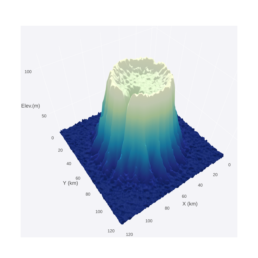
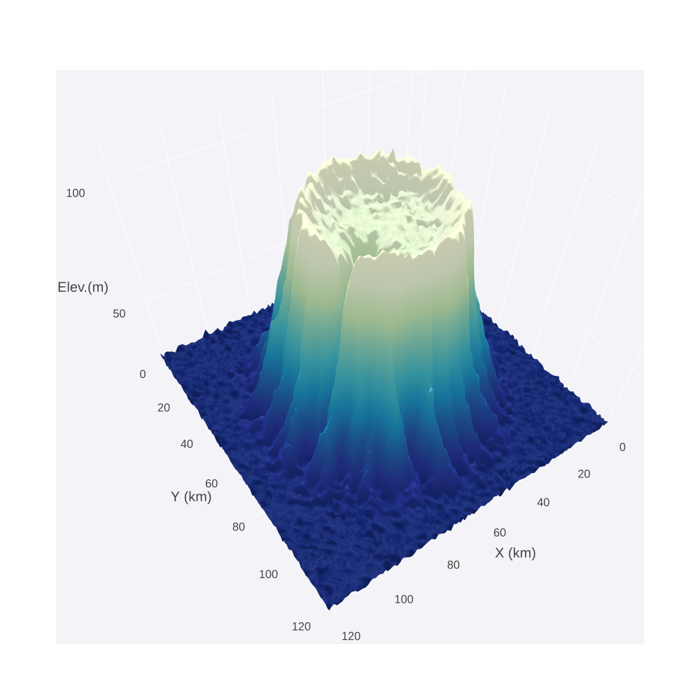
• Cr : We simulate the geomorphological evolution over 50,000 years of a synthetic crater-type topography digital elevation model created by Badlands. The size of the crater is 0.24 x 0.24 kilometers squared. The topography is evaluated at a grid of 123 x 123 points (pixels). The resolution factor which defines the distance between two adjacent points in the grid. In this case, the resolution factor is 0.02 kilometer/point. Figure 1 shows the initial and the final topography after 50,000 years of evolution by Badlands. The final topography is used as the ground-truth topography.

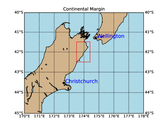
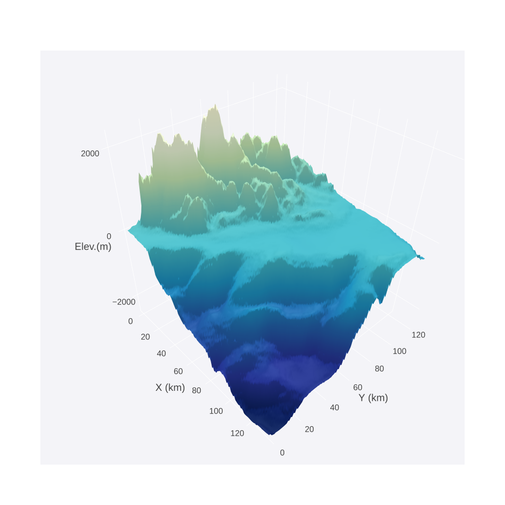
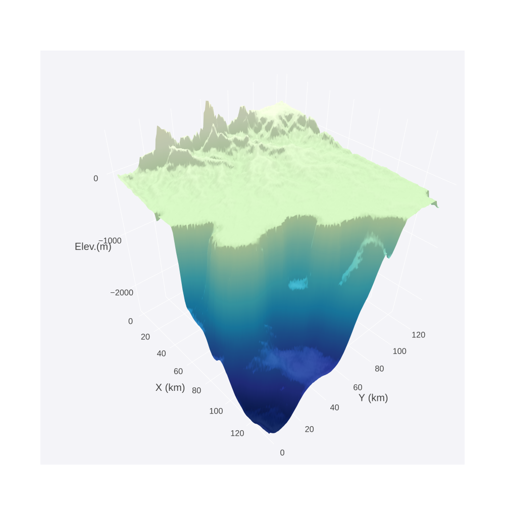
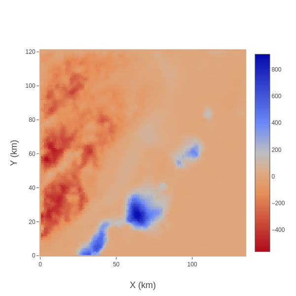
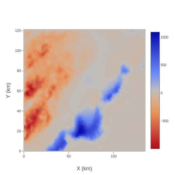
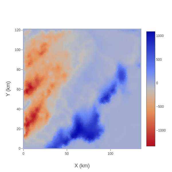
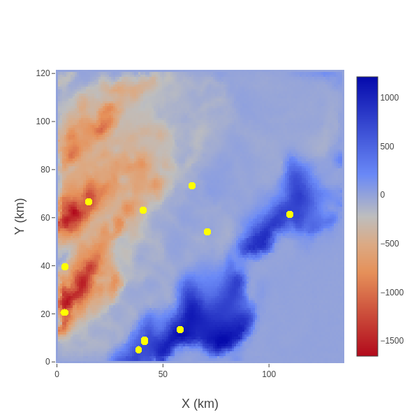
• CM: Using Badlands, we simulate the geomorphological evolution over 1000, 000 years using a real elevation taken from present day South Island in New Zealand as shown in Figure 2. This region is represented by 91 x 81 points that covers 136 by 123 kilometers squared; hence, the resolution factor is 1.5 kilometers/point. Figure 3 shows the initial and the final or ground-truth topography by Badlands. Note that the CM topography is typically a 1 arc-minute global relief model of Earth’s surface that integrates land topography and ocean bathymetry. Figure 4 presents the sediment erosion/deposition for selected time-frames with selected locations used by the Bayeslands framework.

Table 1 shows the set of parameters that were used to create the ground-truth topography described above. We assume the final topographies are observed in the present; by which we imply that the Cr topography began evolution 50,000 years ago while the CM topography began evolution 1000,000 years ago. Hence, the ground-truth or observed topography data ($\boldsymbol{Y}^{obs}$) refers to the topography of present age, where $t=T$. The goal of Bayeslands is to sample and obtain a posterior distribution of the free parameters that governs Badlands. The posterior distribution is used to make inference about the free parameters which includes prediction and uncertainty quantification.

Topography	Time ( $t$ yrs)	$\rho$ (m/yrs)	$\epsilon$	Run-time (s)
Cr	50,000	1.5	5.e-5	0.8
CM	1000,000	1.5	5.e-6	1.1

Table 1: Values used for generation of synthetic ground-truth topographies (Cr and CM). The simulated time that is represented by Badlands is given in years while the run-time for executing a single Badlands model is given in seconds (s).

(a) Cr initial topography

(b) Cr synthetic ground-truth topography

Figure 1: Cr: Initial (panel a) and eroded ground-truth topography (panel b) after 50,000 years.

Figure 2: Map showing the region (highlighted in red) for the Continental-Margin problem selected from the South Island of New Zealand.

(a) CM initial topography

(b) CM ground-truth topography

Figure 3: CM: Initial and eroded ground-truth topography after 1000,000 years.

(a) 250,000 years

(b) 500, 000 years

(c) 750, 000 years

(d) 1,000,000 years

Figure 4: Sediment erosion/deposition for Continental-Margin topography for 4 selected time-frames, panels(a) - (d). Note that the erosion is negative while deposition is positive which is shown by the legend in meters. The yellow points mark the selected locations of the sediment data.

3.2 Bayeslands Model and Priors

3.2.1 Model for topography

In order to implement the model, we take a probabilistic approach and assume that the observed elevation at time $t$, longitude $i$ and latitude $j$, is generated from a signal plus noise model

$$y_{t,i,j}=g_{t,i,j}(\theta)+e_{t,i,j}$$ (5)

where, $y_{t,i,j}$ is the elevation, $g(\boldsymbol{\theta})$ is the signal that depends on the unknown parameters $\theta$, and $e_{i,j}\sim\mathcal{N}(0,\tau^{2})$ is the noise. In this model, $\theta$ is equal to precipitation ($\rho$) and erodibility ($\epsilon$). The notation $N(\mu,\sigma^{2})$ refers to the normal distribution with mean ($\mu$) and variance ($\sigma^{2}$). The noise in Equation (5) reflects the fact that the elevation, at any point in time, will be affected by factors other than those in the Badlands model.

Let $\mathbf{Y}_{T}=(\mathbf{y}_{T,.1},\ldots,\mathbf{y}_{T,.n})$; where, $\mathbf{y}_{T,.j}=(y_{T,1,j},\ldots,y_{T,n,j})^{\prime}$ is the matrix of observed elevations across an $n\times n$ grid of latitude and longitude at time $t$. We place an inverse gamma, $IG(\nu/2,2/\nu)$ prior on $\tau^{2}$ and integrate it out of the likelihood, denoted by $L_{Y_{T}}(\boldsymbol{\theta})$, to give

$$L_{Y_{T}}(\boldsymbol{\theta})\propto\prod_{j=1}^{n}\prod_{i=1}^{n}\left(1+\frac{(y_{T,i,j}-g_{T,i,j})^{2}}{\nu}\right)^{-\frac{\nu+1}{2}}$$ (6)

We note that the mean function $g(\theta)$ has no closed form representation in $\boldsymbol{\theta}$. Therefore, we cannot write down the likelihood as an explicit function of $\boldsymbol{\theta}$. However, given there exists a deterministic relationship between $\boldsymbol{\theta}$ and $g(\boldsymbol{\theta})$, then $P(\mathbf{Y}_{t}|\boldsymbol{\theta},\tau^{2})=P(\mathbf{Y}_{t}|g(\boldsymbol{\theta}),\tau^{2})$. We place uniform priors on precipitation and erodibility, and the limits of the uniform distributions are given in Table 2

Topography	$\rho$[min., max.]	$\epsilon$ [min., max.]
Cr	[0.0-3.0]	[3.e-5, 7.e-5]
CM	[0.0-3.0]	[3.e-6, 7.e-6]

Table 2: Prior range with minimum and maximum values for precipitation ($\phi$) and erodibility ($\epsilon$).

3.2.2 Model for sediment erosion/deposition

Due to the issue of multi-modality in complex models, there can be a number of possible values of $\rho$ and $\epsilon$ which gives rise to the same topography. To constrain the number of possible values, we use information featured in the sediment erosion/deposition history.

As stated previously, we only have ground-truth data of the landscape topography in the present day denoted by $T$. The likelihood given by Equation (6) evaluates the Badlands parameters $\boldsymbol{\theta}$ to ground-truth

topography $y_{T,i,j}$. The estimates for surface topography at previous timescales are often unavailable. However, sedimentary basins contain a record of erosion and deposition which is available as total sediment thickness of as a stratigraphic sequence; i. e. sediment thickness through space and time, for $t<T$. Therefore, the information from sedimentary deposits can be incorporated into the likelihood. Let $z_{t,j}$ be the thickness of the sediment at time $t$, at location $j$. We assume this deposition also depends upon $\boldsymbol{\theta}$ via a signal plus noise model whereby

$$z_{t,j}=f_{t,j}(\boldsymbol{\theta})+\eta_{t,j}$$

where, $f(\boldsymbol{\theta})$ is the signal that represents sediment thickness given by the Badlands model, for a given value of $\boldsymbol{\theta}$ and $\eta\sim\mathcal{N}(0,\sigma^{2})$ is the noise. Analogous to the topography data, we integrate out $\sigma^{2}$ and the likelihood function for the sediment data, $L_{Z}(\boldsymbol{\theta})$ is given by

$$L_{Z}(\boldsymbol{\theta})\propto\prod_{t=1}^{n_{t}}\prod_{j=1}^{m}\left(1+\frac{(z_{t,j}-f_{t,j})^{2}}{\nu}\right)^{-\frac{\nu+1}{2}}$$ (7)

where, $n_{t}$ is the number of times that the sediment thickness is recorded and $m$ is the number of points at which the sediment is measured.

3.3 Bayeslands framework

We take a Bayesian approach and estimate the topography via Badlands using the

posterior mean of the selected parameters, $E(y^{*}_{T,i,j}|\mathbf{Z}_{t},\mathbf{Y}_{T})$. The posterior mean is equal to

$$E(y^{*}_{T,i,j}|\mathbf{Z},\mathbf{Y}_{T}) = \int E(y^{*}_{Tij}|\mathbf{Y}_{T},\boldsymbol{\theta})p(\boldsymbol{\theta}|\mathbf{Z}_{t},\mathbf{Y}_{T})d\boldsymbol{\theta}\$$

and an estimate of it is

$$\hat{E}(y^{*}_{T,i,j}|\mathbf{Z},\mathbf{Y}_{T}) = \frac{1}{M}\sum_{j=1}^{M}E(y^{*}_{T,i,j}|\mathbf{\mathbf{missing}}Z_{t},Y_{T},\boldsymbol{\theta}^{[j]})$$ (8)

where, $\boldsymbol{\theta}^{[j]}\sim p(\boldsymbol{\theta}|\mathbf{Y})$ is obtained via MCMC in Bayeslands as shown in Algorithm  1. That is we draw each element of $\theta$ from a proposal distribution, $q(\theta|\theta^{c}),$ conditional on the current value of $\theta$, denoted by $\theta^{c}$. The proposed value of $\theta^{p}$ is accepted with probability

$$\alpha=\min\left\{1,\frac{L_{Y_{T}}(\boldsymbol{\theta}^{p})L_{Z}(\boldsymbol{\theta}^{p})}{L_{Y_{T}}(\boldsymbol{\theta}^{c})L_{Z}(\boldsymbol{\theta}^{c})}\right\}$$ (9)

which ensures the convergence of the chain to its stationary distribution, $p(\theta|\mathbf{Y},\mathbf{Z})$. Note that as $q(.)$ is symmetric and $p(\boldsymbol{\theta})$ is the product of independent uniform priors, $\alpha$ reduces to the likelihood ratio. The inference regarding the selected parameters are given via the joint posterior $p(\boldsymbol{\theta}|\mathbf{Y},\mathbf{Z})$.

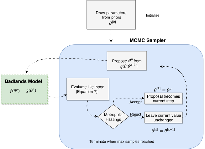
Figure 5 gives an overview of the Bayeslands framework that employs the MCMC sampler for the Badldands model. Algorithm 1 begins by initializing values of precipitation and erodibility by drawing from the respective prior distribution for the selected parameters given in Table 2. The algorithm then proceeds by proposing new values of the parameter (Step 1) from the normal distribution as the proposal distribution, with mean $\boldsymbol{\theta}^{[i-1]}$ and the step-size ($\phi_{p}$ and $\phi_{\epsilon}$ ). Conditional on these proposed values, Badlands is executed for the maximum time (eg. Cr=50,000 years) which produces outputs that include the successive sediment erosion/deposition and topographies (Step 2). The choice of a random-walk proposal distribution was due to the unavailability of gradients for the selected parameters in the Badlands model. Then the likelihood given by Equation (7) is evaluated by considering the final topography and the successive erosion deposition values at selected locations (e.g. Figure 4). Once the likelihood is computed, the Metropolis-Hasting criterion is used for determining whether to accept or reject the proposal (Step 3). If the proposal is accepted, the chain moves to this proposed value. If rejected, the chain stays at the current value (Step 4). The process is repeated until the convergence criterion is met, which in this case is the maximum number of samples defined by the user. Note that the software package in Python along with data is given online .

Figure 5: Bayeslands framework employing MCMC random-walk sampler and Badlands model. Further details are given in Algorithm 1.

Algorithm 1 Bayeslands framework

Initialize $\boldsymbol{\theta}=\boldsymbol{\theta}^{[0]}$ by drawing $\boldsymbol{\theta}^{[0]}$ from the prior $\boldsymbol{\theta}^{[0]}\sim p(\boldsymbol{\theta})$
For $i=1:Samples$

1:Propose a value $\boldsymbol{\theta}^{[p]}|\boldsymbol{\theta}^{i-1}\sim q(\boldsymbol{\theta}^{[i-1]})$, where $q(.)$ is the proposal distribution.

2:Given $\boldsymbol{\theta}^{[p]}$, execute Badlands and compute $g_{Tmax,i,j}\left(\boldsymbol{\theta}^{[p]}\right)$, and $f_{t,i,j}\left(\boldsymbol{\theta}^{[p]}\right)$

3:Calculate the acceptance probability $\alpha$, as given by Equation 9.

4:Generate $u\sim U(0,1)$ and set $\boldsymbol{\theta}^{[i]}=\boldsymbol{\theta}^{[p]}$ if $\alpha<u$. Otherwise, set $\boldsymbol{\theta}^{[i]}=\boldsymbol{\theta}^{[i-1]}$.

3.4 Experimental setting and evaluation

In order to evaluate the performance of Bayeslands on the problems (CM and Cr) presented previously, we consider the following issues and metrics:

1. Visualization of the true posterior surface evaluated across the grid;

2. Bayeslands MCMC sampling and posterior distributions;

3. Prediction of the topography and sediment erosion/deposition.

We present the metrics for evaluating Bayeslands using the Badlands outputs (predicted topography and sediment erosion/deposition). We highlight that although a series of topographies are generated by Badlands, only the final topography is used for evaluation, while selected sediment erosion/deposition is used. The root mean squared-error (RMSE) is used as the metrics for evaluation where the final topography elevation (elev) and sediment erosion/deposition (sed) respectively are given by

$$\mbox{RMSE}_{elev} = \sqrt{\frac{1}{n\times m}\sum_{i=1}^{n}\sum_{j=1}^{n}\left(g(\hat{\theta}_{T,i,j})-g_{T,i,j}(\theta)\right)^{2}}$$

$$\mbox{RMSE}_{sed} = \sqrt{\frac{1}{n_{t}\times v}\sum_{t=1}^{n_{t}}\sum_{j=1}^{m}\left(f(\hat{\theta}_{t,j})-f(\theta_{t,j})\right)^{2}}$$

where, $\hat{\theta}$ is an estimated value of $\theta$, chosen according to some criteria and $\theta$ is the true value on which the ground truth topographies and sediment thickness were based. $f(.)$ and $g(.)$ represent the outputs of the Badlands model, as defined earlier while $m$ and $n$ represent the size of the selected topography. $v$ is the total number of selected points from sediment erosion/deposition as shown in Figure 4 over the selected time frame, $n_{t}$.

We use the information about uniform priors for the respective parameters from Table 2. We construct proposal distributions using a covariance matrix, which is assumed to be diagonal with entries equal to the square of step-size ($\phi$). We performed several trial experiments to evaluate an optimal $\phi$ and use $\phi_{\rho}=0.03$ for precipitation for both cases (Cr and CM). In the case for erodibility, CM uses $\phi=4.e-8$ while Cr uses $\phi_{\epsilon}=4.e-7$. We evaluate Bayeslands for selected number of samples with a 10% burn-in period. Note that burn-in is considered as the initial sampling period before the draws in the chain are assumed to be from the invariant distribution, which in this case is the joint posterior. The different number of samples are used to check the convergence properties of the MCMC.

The overall computation time taken for Bayeslands for each experiment is also reported. We use an Intel Core i7-8700 Processor (Hexa-core, 3.2 Giga-Hertz) for all the experiments. Note that parallel computing was not used in the implementation of Bayeslands.

4 Results

4.1 Visualization of the true posterior surface

(a) Cr true posterior surface

(b) CM true posterior

Figure 6: True posterior (log-likelihood) surfaces for Cr and Continental-Margin topography as a function of precipitation $\rho$ and epsilon $\epsilon$ obtained by a grid-search.

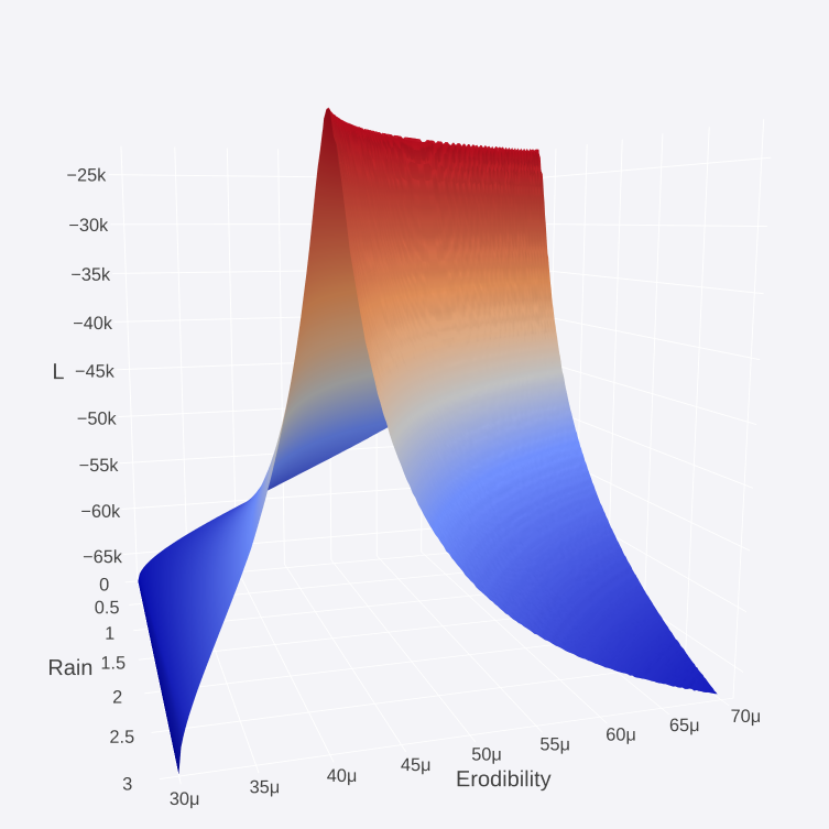
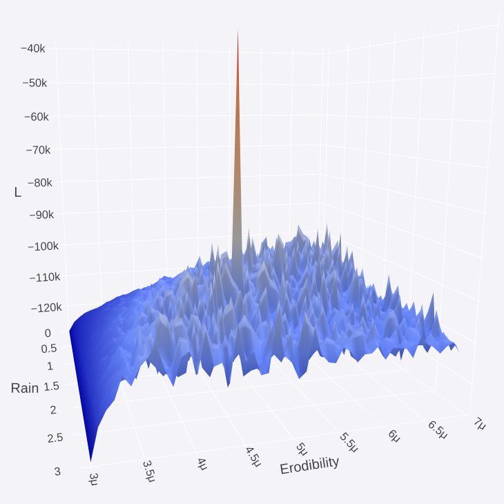
To illustrate the difficulty of making inference in geophysical inversion problems, we produce the posterior surface (up to a proportionality constant), evaluated across a grid of values for $\rho$ and $\epsilon$. We note that it is only computationally and visually possible to produce these plots for very low dimensional problems, and yet these surfaces demonstrate the challenges of MCMC sampling. Figure 6 panel (a) presents the posterior surface for the Cr topography and shows that this surface is more sensitive to erodibility than precipitation. It also shows that there is no unique mode for precipitation and erodibility. Several combinations of precipitation and erodibility give the same posterior value, indicated by the ridge. Figure 6 panel (b) presents the posterior surface for CM which is in sharp contrast to the posterior surface for the Cr. Although it shows the existence of a unique global maximum, there are a number of local maxima, which makes the exploration of the surface very challenging.

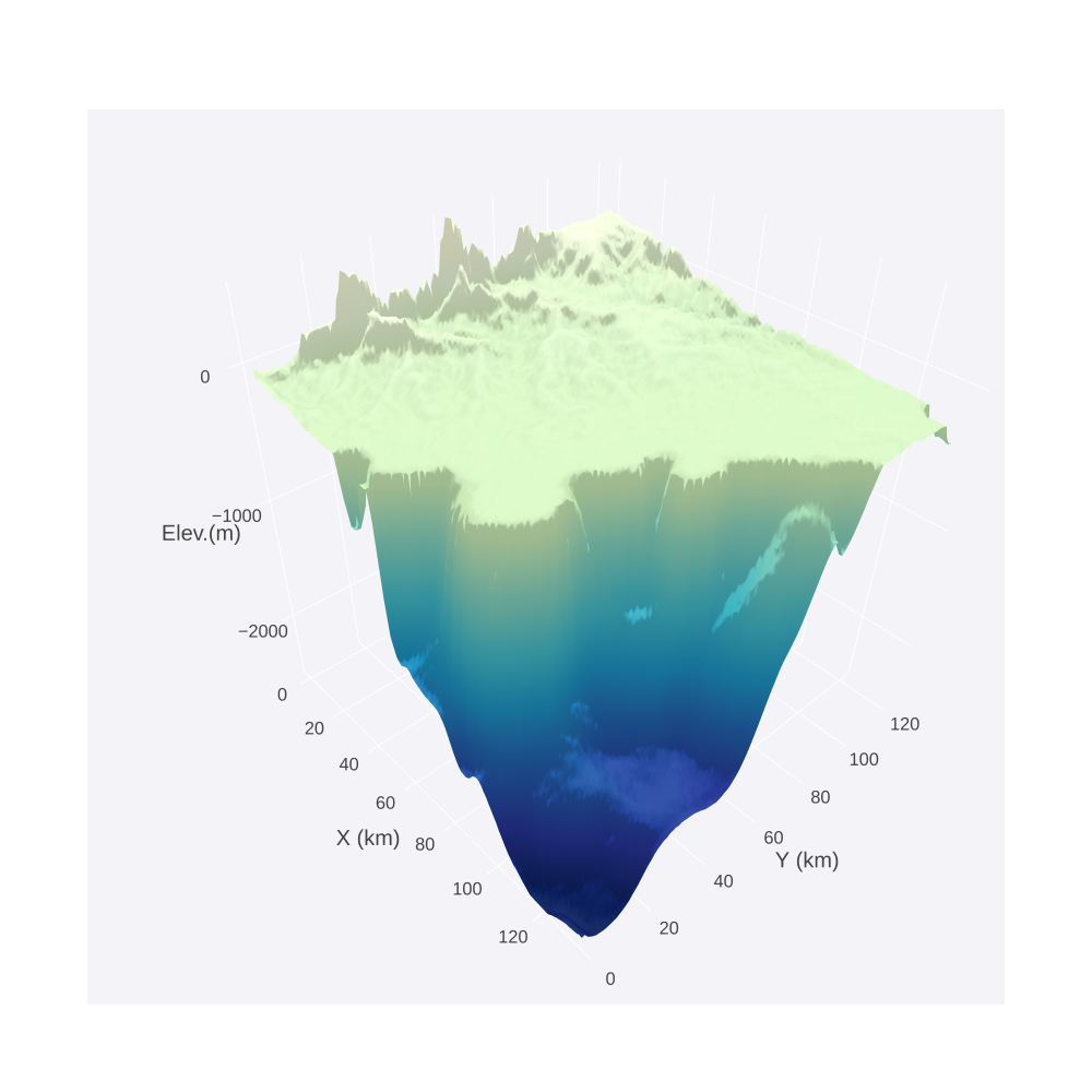
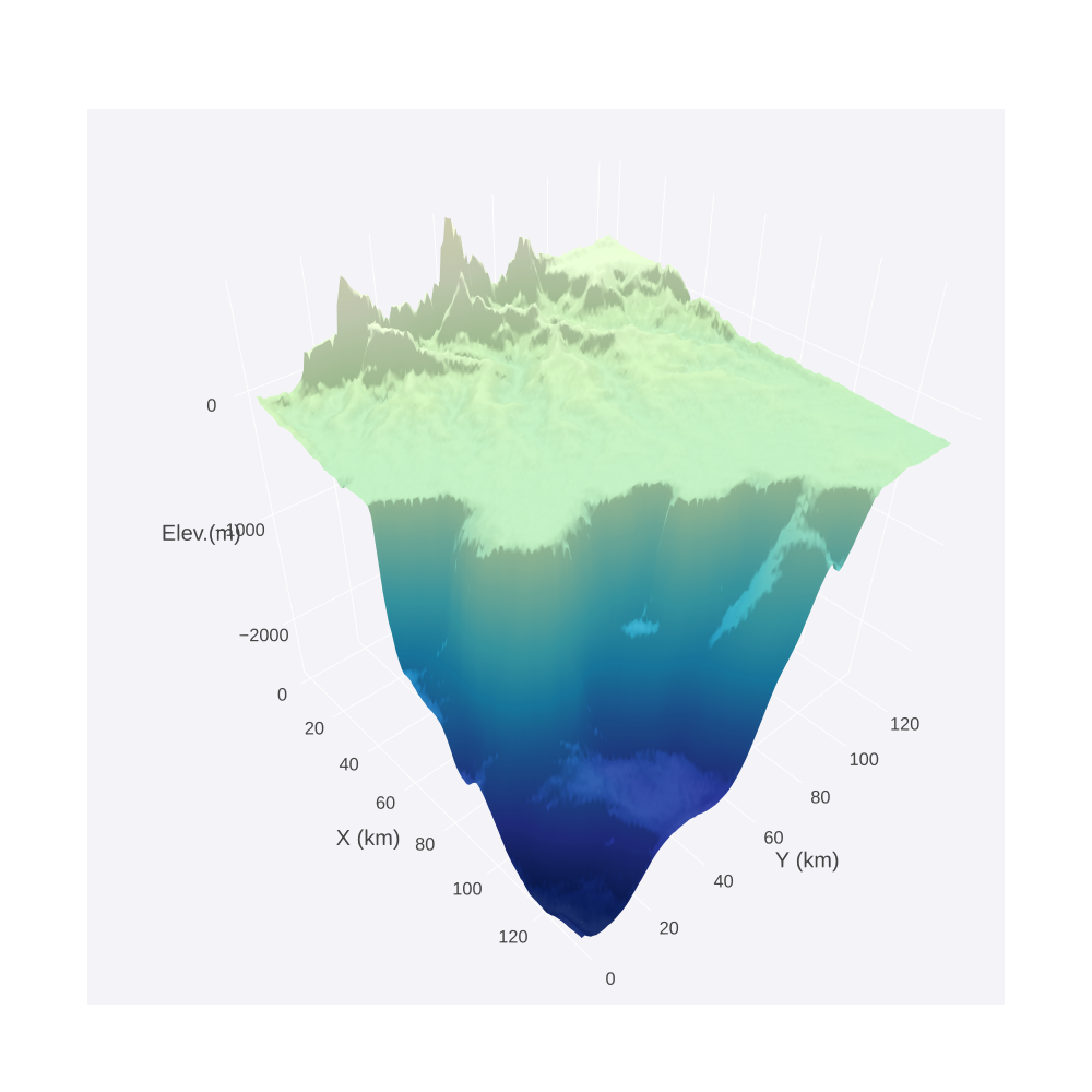
Table 3 presents the top 10 combinations of the parameters with minimal RMSE values. Note that the first combination (true-value) shows the actual values that were used to generate the ground-truth topography, hence the corresponding RMSE values are 0. Figures 7 and 8 give a visualization of the ground truth topography. Panel (a) corresponds to the topography giving the lowest RMSE, while panel (b) corresponds to the topography with the $5^{th}$ lowest RMSE. It can be seen that there is not much difference between the sub-optimal and optimal values, particularly for the CM problem in Figure 8.

Combinaton	Topography	Precipitation	Erodibility	$RMSE_{elev}$	$RMSE_{sed}$	$RMSE_{total}$
True-value	Cr	1.50	5.00e-5	0.00	0.00	0.00
1		1.14	5.72e-5	1.05	0.26	1.31
2		2.94	3.56e-5	1.05	0.26	1.32
3		2.40	3.96e-5	1.04	0.27	1.32
4		2.58	3.80e-5	1.05	0.26	1.32
5		1.98	4.36e-5	1.04	0.27	1.32
6		0.78	6.92e-5	1.06	0.26	1.32
7		2.28	4.04e-5	1.05	0.27	1.32
8		1.08	5.88e-5	1.06	0.26	1.32
9		1.02	6.04e-5	1.05	0.27	1.32
10		0.90	6.44e-5	1.07	0.26	1.32
True-value	CM	1.50	5.00e-6	0.00	0.00	0.00
1		2.64	3.96e-6	69.85	27.63	97.48
2		2.70	4.20e-6	69.71	28.55	98.26
3		1.38	4.68e-6	69.84	33.44	103.20
4		2.10	4.28e-6	68.59	42.70	111.35
5		2.58	3.40e-6	73.42	42.97	116.43
6		2.34	4.04e-6	102.2	15.30	117.51
7		2.94	3.88e-6	79.58	40.55	120.10
8		2.76	3.64e-6	104.61	15.64	120.35
9		1.20	5.56e-6	69.45	51.14	120.51
10		0.78	6.76e-6	105.72	27.98	123.77

Table 3: Columns 3-4 are combinations of parameters of precipitation $\rho$ and erodibility $\epsilon$ that give near optimal performance, in terms of $RMSE_{t}otal$, for Cr, top panel, and CM bottom panel.

(a) Cr (true value from Table 3)

(b) Cr topography (Combination 1 from Table 3)

(c) Cr topography (Combination 5 from Table 3)

Figure 7: Cr: Selected cases showing that there is not much difference between the different combinations (unique modes) of the parameters when compared to the true-values.

(a) CM (true value)

(b) CM topography (Combination 1)

(c) CM topography (Combination 5)

Figure 8: CM: Selected cases showing that there is not much difference between the different combinations (sub-optimal modes) of the parameters when compared to the true-values.

4.2 Inference using Bayeslands

Table 4 gives details on the number of iterations (samples) in the MCMC sampling scheme, the the corresponding time taken, and the prediction performance as measured by $RMSE_{elev}$ and $RMSE_{sed}$ and their total, $RMSE_{total}$. We find that $\mbox{RMSE}_{total}$ decreased (improved) with the increase in sample size from 10,000 to 50,000 for the Cr topography. This improvement is in both $\mbox{RMSE}_{elev}$ and $\mbox{RMSE}_{sed}$, suggesting that the MCMC scheme for this landscape had not converged within the first 10,000 samples.A similar tend is seen in the the CM topography.

Topography	Samples	Accepted %	Time (hours)	$\mbox{RMSE}_{elev}$	$\mbox{RMSE}_{sed}$	$\mbox{RMSE}_{total}$
Cr	10,000	2.35	2.26	3.69	4.56	8.25
	25,000	0.28	5.43	3.10	4.34	7.44
	50,000	0.22	8.68	1.26	0.95	2.21
CM	10,000	0.47	4.20	133.90	83.28	217.20
	25,000	0.05	10.66	131.5	62.64	194.10
	50,000	0.04	19.29	94.26	29.69	123.90

Table 4: Results for Bayeslands MCMC sampling

(a) Trace-plot of accepted samples

(b) Posterior distribution

Figure 9: Cr: Panel (a) is a trace plot of the Cr precipitation ($\rho$) posterior for 50,000 samples, while panel (b) is a histogram estimate of the posterior distribution. The vertical red line shows true value.

(a) Trace-plot of accepted samples

(b) Posterior distribution

Figure 10: Panel (a) is a trace plot of the CM precipitation ($\rho$) posterior for 50,000 samples, while panel (b) is a histogram estimate of the posterior distribution. The vertical red line shows true value.

(a) 12,500 years

(b) 25,000 years

(c) 37,500 years

(d) 50,000 years

Figure 11: Cr: Predicted topographies at selected intervals for 50,000 years.

(a) 250,000 years

(b) 500,000 years

(c) 750,000 years

(d) 1000,000 years

Figure 12: CM topography evolution over time at selected intervals for 1000,000 years.

(a) Elevation cross-section along x-axis

(b) Elevation cross-section along y-axis

Figure 13: Cr: Elevation cross-section taken at mid-point along x-axis and y-axis.The green shaded area corresponds to 95% credible intervals.

(a) Elevation cross-section along x-axis

(b) Elevation cross-section along y-axis

Figure 14: CM model: Panel (a), elevation cross-section from West to East at a latitude of $42\degree$. Panel (b), elevation cross-section from North to South at a longitude of 174°. The green shaded area shows 95% credible interval.

(a) 250,000 years

(b) 500,000 years

(c) 750,000 years

(d) 1000,000 years

Figure 15: CM: Sediment erosion/deposition for selected time-frames fand locations for 1,000,000 years. The selected locations (ID) are shown in Figure 4.

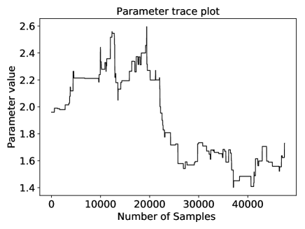
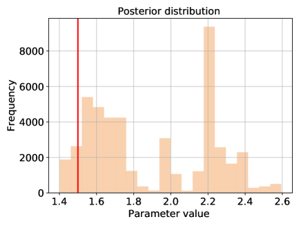
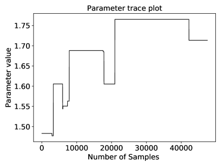
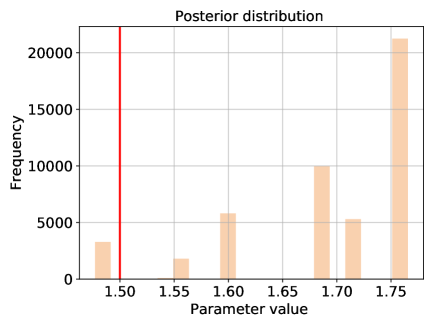
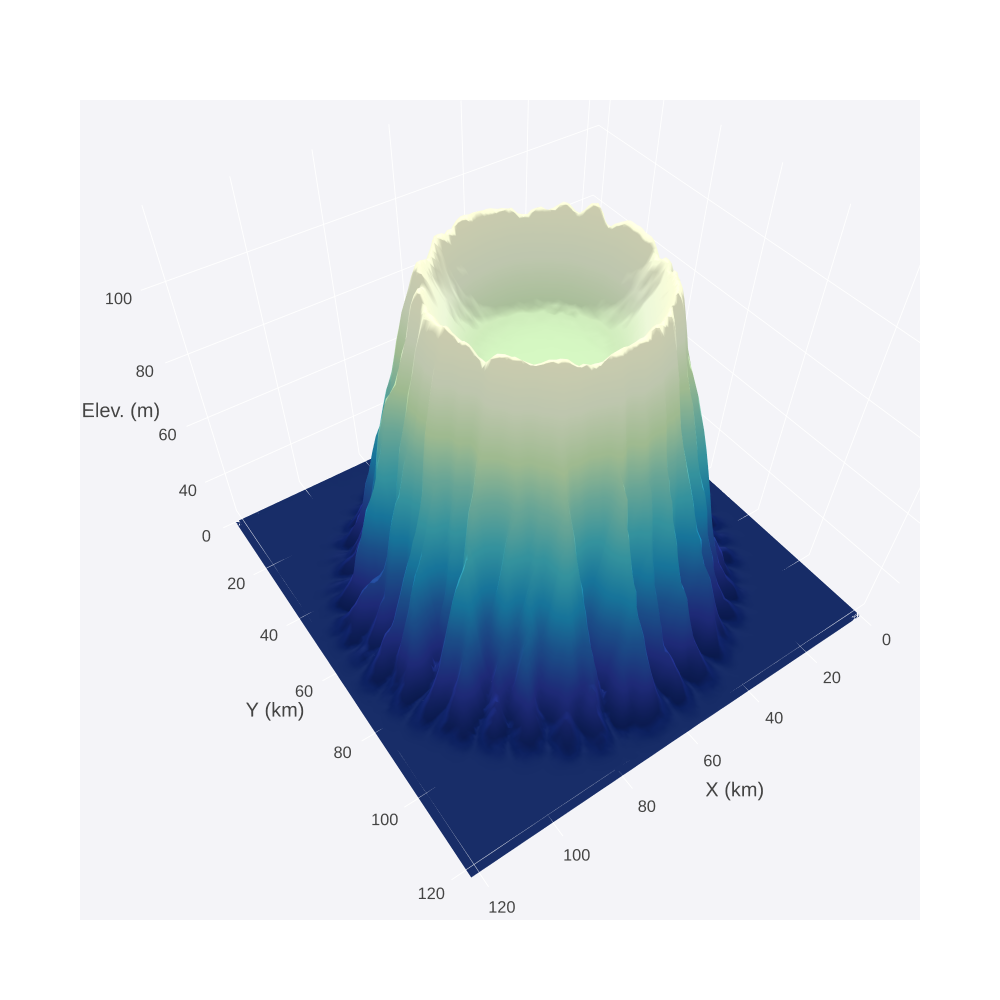
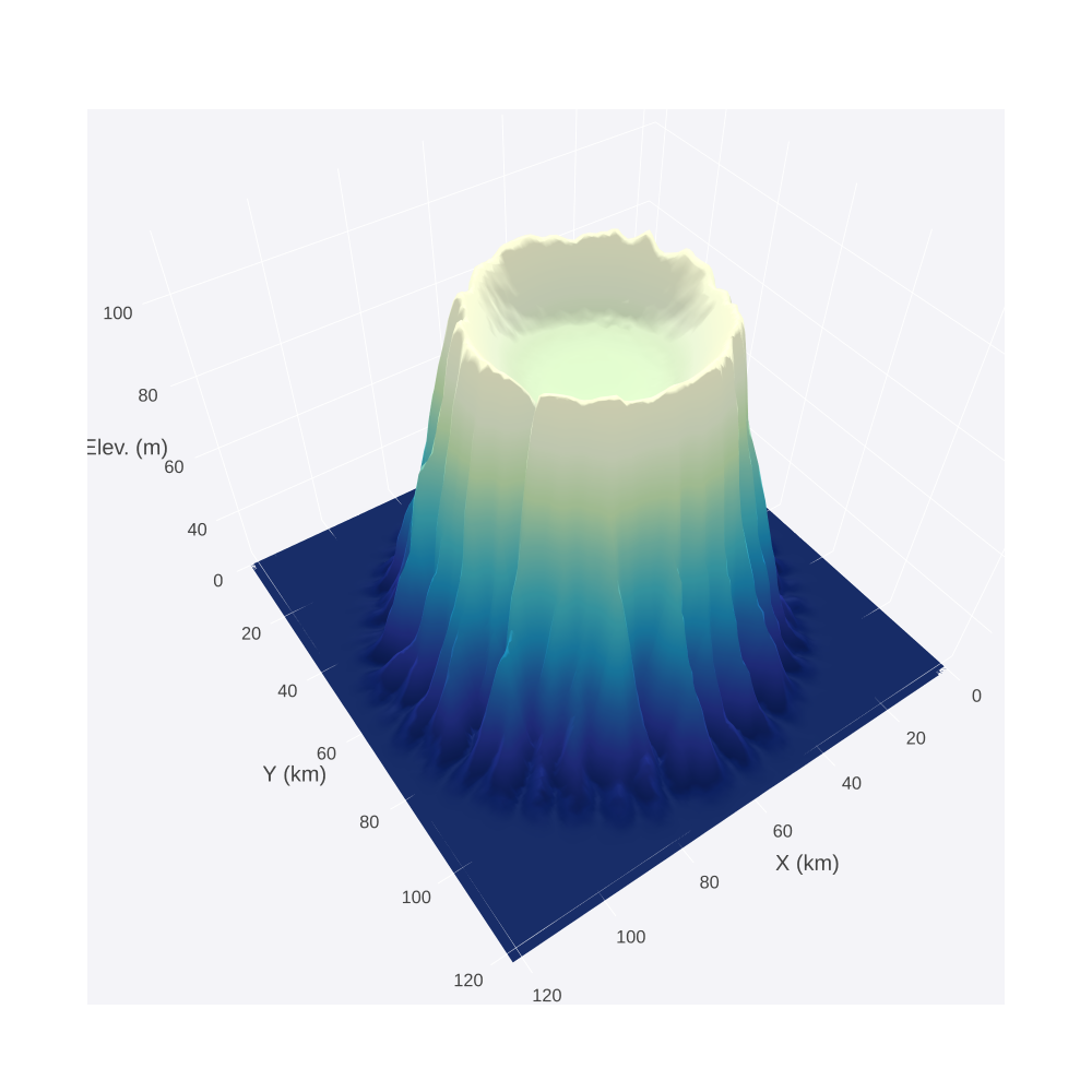
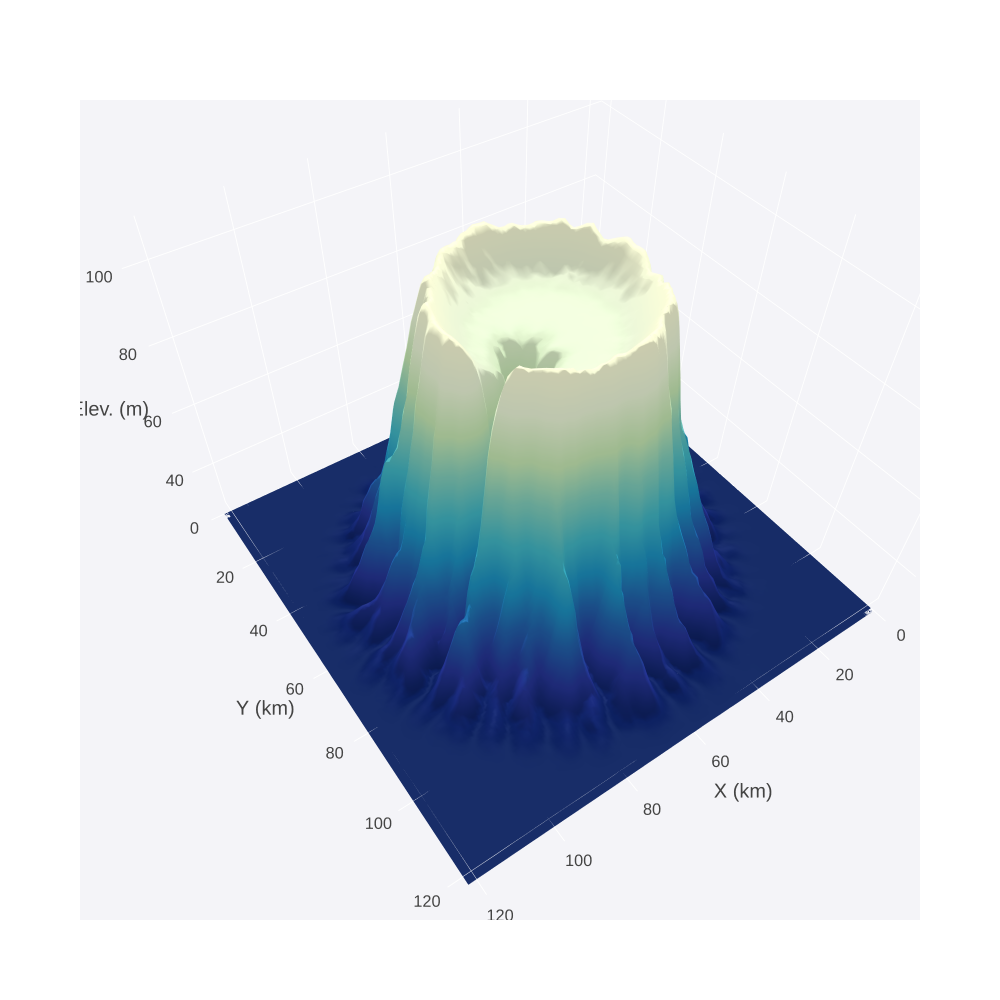
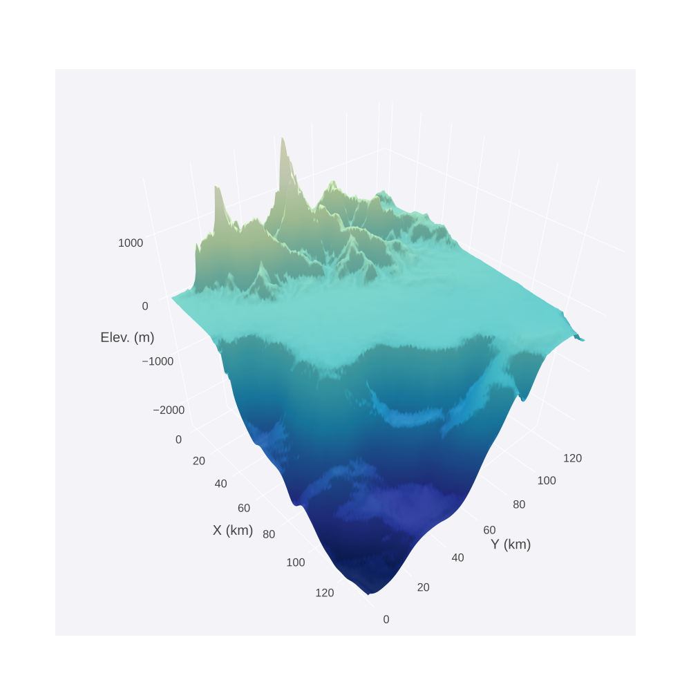
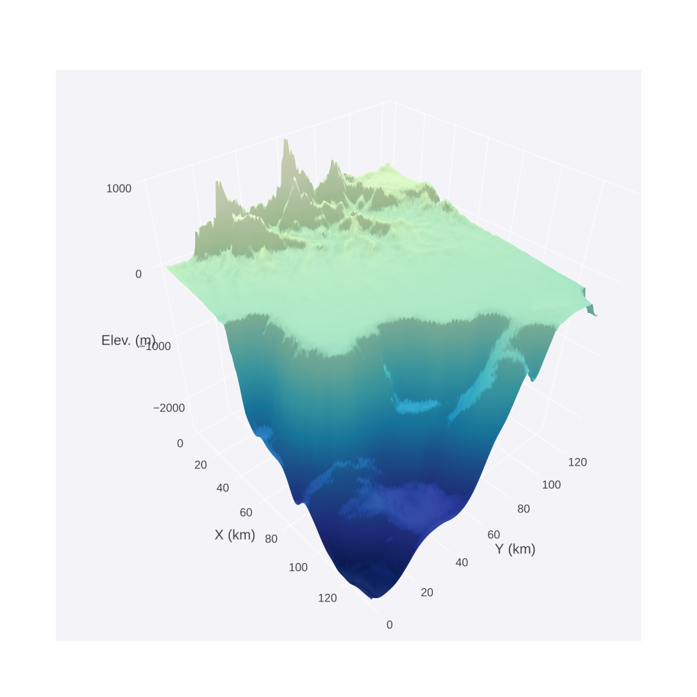
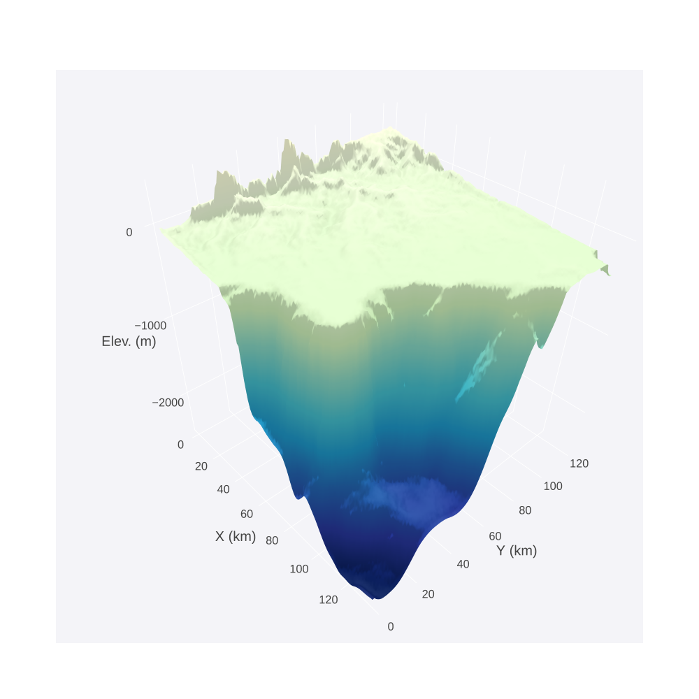
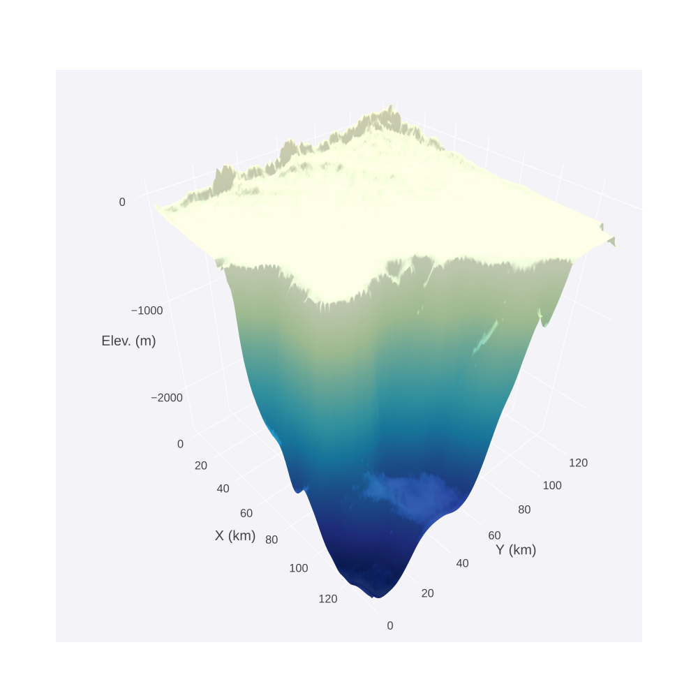
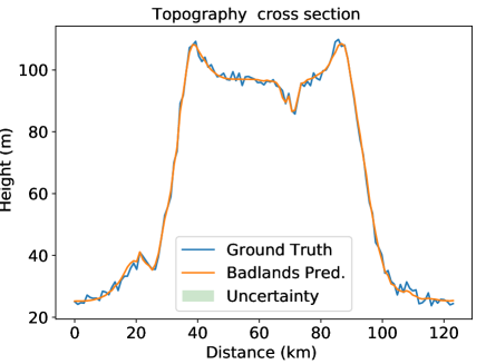
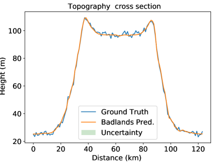
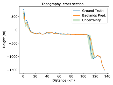
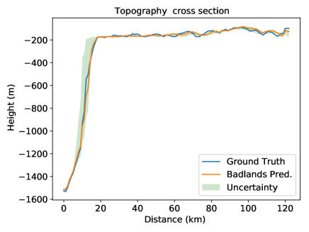
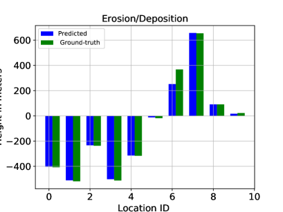
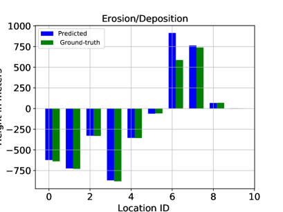
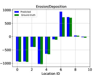
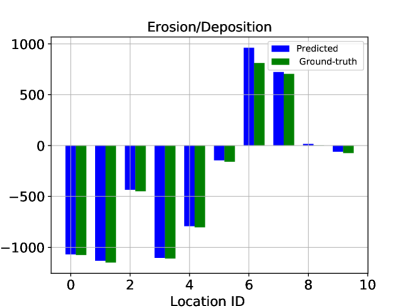
Figure 9, panel(a) shows the trace plot of accepted proposals in MCMC sampling for precipitation $\rho$, while panel (b) is a histogram estimate of the posterior distribution for the Cr topography. Note that the vertical line in red in the respective figures shows the true value and the major goal of the experiments was to check if Bayeslands framework can recover the true value. In the case of the Cr topography, we find that the MCMC sampling estimate of the posterior distribution is reasonable. It has one of the modes near the true values of precipitation and erodibility the MCMC chain appears to mix well, although with a high degree of auto-correlation. We note that the MCMC sampling recovered few different modes as reported by the trace plot of the posterior distribution. In contrast, the CM topography (Figures  10) MCMC sampling procedure shows that the chains have difficulty in escaping local modes, hence they are stuck (shown in the trace-plot) for longer time periods when compared to the Cr topography trace-plots. As evident by the trace plots, there little mixing. The histogram estimates of precipitation and erodibility are not peaked around the true values for these parameters. Instead they are multimodal with modal values corresponding to local maxima, given by the coloured dashed vertical lines. The difference in these results are not surprising, when one considers that the CM topography’s likelihood surface is very complex when compared with that of the Cr, resulting in the need for longer sampling time and better or adaptive MCMC proposal schemes from better traversal.

Despite the difficulty in recovering the true parameter values, the prediction for the landscape topographies are astonishingly accurate. This is evident from the predicted topography; Figures 11 and 12 which are visually similar to the ground truth, Figures 1 and 3. Moreover, the cross-sections shown in Figures 13 and 14 show good accuracy with 95% credible interval which highlight the accuracy of the prediction. Figure 15 shows the predicted evolution of the sediment thickness for both topographies. Interestingly, the CM predictions appear to be more accurate than those of the Cr landscape. However this may be due to the different scales. We note that the sediment thickness of the Cr topography is two orders of magnitude less than that of CM which makes differences appear larger.

5 Discussion

In this paper, we presented a logically consistent Bayesian framework to estimate and quantify uncertainty for selected parameters that govern LEMs. This was achieved by embedding a LEM (Badlands) within a probabilistic model. Although we used Badlands, we stress that the approach is general; it can accommodate any LEM and other geophysical forward models where the outputs are a deterministic function of the inputs, for instance Underworld models to explore the geothermal potential of the crust [51].

We made inference for only 2 free parameters (precipitation and erodibility) and assumed that they were constant over space and time. Even with this simplification, Figure 6 shows that the posterior (likelihood) surfaces are non-standard and difficult to estimate. Multi-modality [52] in the posterior distribution is a major concern. Multi-modality shows that multiple combinations of the given parameters (precipitation and erodibility) can plausibility predict or simulate the same topography, which closely resembles the synthetic or ground-truth topography [53] (e.g. Figure 8 and Table 3). In addition to the issue of multi-modality, the posterior may be discontinuous, by which we mean the derivative does not exist which further makes MCMC sampling difficult.

Which aspects of the problem give rise to these unusual posterior surfaces? Are these surfaces a product of the data or due to complexity of the Badlands model? It is important to reflect upon the characteristics or assumptions made in geophysical models, characteristics of the topography data for a given time and location. It is worthwhile to investigate if the posterior distribution gives meaningful information about the appropriateness of the Badlands model to different topographies.

Clearly, limiting precipitation and erodibility to be constant for the entire spatial and temporal extent of a given model may not be appropriate. While this may not make much difference for small geographical regions and short time intervals; for larger areas, different regions of the topography would have different distributions of precipitation at different points of time. Moreover, the parameter values are also same throughout the entire topography evolution. This does not fully simulate geological time scales and fully capture the effects of changing climate through time. In order to implement this, the precipitation would become a vector of parameters that define different regions expressed by grids in the map. This would increase the number of parameters and further add complexity to the model which would make the inference more difficult. Furthermore, the synthetic problems should consider larger areas that contain a variety of landscape features. This would increase the computational complexity of the model and require multi-core implementations of MCMC via high performance computing. Parallel tempering [54], which is an advanced MCMC method suited for multi-core implementation that better captures multi-modality, would be a natural choice to improve the performance of the sampler [23, 55].

The Bayeslands framework will form the foundation for more complex models of landscape and basin evolution. In the future, we envision to include many additional parameters in Bayeslands, including the uncertain initial model topography, global sea level fluctuations, tectonic and dynamic topography evolution, spatially varying lithospheric flexural rigidity, spatio-temporal variations in mountain uplift rates and in precipitation. Ultimately, we will be able to consider the uncertain effects of climate change and changing vegetation cover on spatio-temporal denudation rates and improve assessments on how re-vegetation may slow down the continuing erosion of degraded landscapes [56].

6 Conclusions and Future Work

Bayeslands provides a framework for incorporating uncertainty quantification for simulated elevation and sediments in Badlands through MCMC sampling in landscape evolution models. Although promising, there are major challenges in scaling to higher dimensions which are characteristic of real-world applications. As the dimension increases, there can be further challenges with issues of multi-modality and exploration in such posterior distributions. The exploration of these challenging posterior distributions will require the development of new proposal distributions for use in MCMC schemes, which reflect local geometry and/or gradient information from the Badlands model.

The Bayeslands framework can be computationally challenging since Badlands takes minutes to hours for large scale or continental problems. Hence, new computationally efficient methods, such as replacing the Badlands model with surrogate models for a proportion of the MCMC iterates needs to be developed. Speeding up computation of Bayeslands via parallel tempering in multi-core architecture is another avenue to be explored in the future.

7 References

References

- [1] N. Flament, M. Gurnis, R. D. Müller, A review of observations and models of dynamic topography, Lithosphere 5 (2) (2013) 189–210.
- [2] J. Braun, M. Sambridge, Modelling landscape evolution on geological time scales: a new method based on irregular spatial discretization, Basin Research 9 (1) (1997) 27–52.
- [3] T. Coulthard, Landscape evolution models: a software review, Hydrological processes 15 (1) (2001) 165–173.
- [4] K. X. Whipple, G. E. Tucker, Implications of sediment-flux-dependent river incision models for landscape evolution, Journal of Geophysical Research: Solid Earth 107 (B2) (2002) 1–20.
- [5] G. Tucker, G. R. Hancock, Modelling landscape evolution., Earth Surf. Process Landf. 35 (1) (2010) 28–50.
- [6] T. Salles, G. Duclaux, Combined hillslope diffusion and sediment transport simulation applied to landscape dynamics modelling., Earth Surf. Process Landf. 40 (6) (2015) 823–39.
- [7] B. Campforts, W. Schwanghart, G. Govers, Accurate simulation of transient landscape evolution by eliminating numerical diffusion: the ttlem 1.0 model, Earth Surface Dynamics 5 (1) (2017) 47–66.
- [8] J. M. Adams, N. M. Gasparini, D. E. J. Hobley, G. E. Tucker, E. W. H. Hutton, S. S. Nudurupati, E. Istanbulluoglu, The landlab v1.0 overlandflow component: a python tool for computing shallow-water flow across watersheds, Geoscientific Model Development 10 (4) (2017) 1645–1663.
- [9] F. J. Pazzaglia, Landscape evolution models, Developments in Quaternary Sciences 1 (2003) 247–274.
- [10] A. Chen, J. Darbon, J.-M. Morel, Landscape evolution models: A review of their fundamental equations, Geomorphology 219 (2014) 68–86.
- [11] T. Salles, Badlands: A parallel basin and landscape dynamics model, SoftwareX 5 (2016) 195–202.
- [12] T. Salles, N. Flament, D. Müller, Influence of mantle flow on the drainage of eastern australia since the jurassic period, Geochemistry, Geophysics, Geosystems 18 (1) (2017) 280–305.
- [13] L. R. Scott, S. Zhang, Finite element interpolation of nonsmooth functions satisfying boundary conditions, Mathematics of Computation 54 (190) (1990) 483–493.
- [14] V. Godard, J. Lavé, R. Cattin, Numerical modelling of erosion processes in the himalayas of nepal: Effects of spatial variations of rock strength and precipitation, Geological Society, London, Special Publications 253 (1) (2006) 341–358.
- [15] J. Rejman, R. Turski, J. Paluszek, Spatial and temporal variations in erodibility of loess soil, Soil and Tillage Research 46 (1-2) (1998) 61–68.
- [16] Z. Chair, P. K. Varshney, Distributed Bayesian hypothesis testing with distributed data fusion, IEEE transactions on systems, man, and cybernetics 18 (5) (1988) 695–699.
- [17] C. Notarnicola, F. Posa, Bayesian fusion of active and passive microwave data for estimating bare soil water content, in: Geoscience and Remote Sensing Symposium, 2001. IGARSS’01. IEEE 2001 International, Vol. 3, IEEE, 2001, pp. 1167–1169.
- [18] W. Moon, C. So, Information representation and integration of multiple sets of spatial geoscience data, in: Geoscience and Remote Sensing Symposium, 1995. IGARSS’95.’Quantitative Remote Sensing for Science and Applications’, International, Vol. 3, IEEE, 1995, pp. 2141–2144.
- [19] W. K. Hastings, Monte carlo sampling methods using markov chains and their applications, Biometrika 57 (1) (1970) 97–109.
- [20] N. Metropolis, A. W. Rosenbluth, M. N. Rosenbluth, A. H. Teller, E. Teller, Equation of state calculations by fast computing machines, The journal of chemical physics 21 (6) (1953) 1087–1092.
- [21] A. Malinverno, Parsimonious Bayesian markov chain monte carlo inversion in a nonlinear geophysical problem, Geophysical Journal International 151 (3) (2002) 675–688.
- [22] K. Mosegaard, A. Tarantola, Monte carlo sampling of solutions to inverse problems, Journal of Geophysical Research: Solid Earth 100 (B7) (1995) 12431–12447.
- [23] M. Sambridge, Geophysical inversion with a neighbourhood algorithm II. appraising the ensemble, Geophysical Journal International 138 (3) (1999) 727–746.
- [24] M. K. Sen, P. L. Stoffa, Global optimization methods in geophysical inversion, Cambridge University Press, 2013.
- [25] K. Gallagher, K. Charvin, S. Nielsen, M. Sambridge, J. Stephenson, Markov chain monte carlo (MCMC) sampling methods to determine optimal models, model resolution and model choice for earth science problems, Marine and Petroleum Geology 26 (4) (2009) 525–535.
- [26] A. Jasra, D. A. Stephens, K. Gallagher, C. C. Holmes, Bayesian mixture modelling in geochronology via markov chain monte carlo, Mathematical Geology 38 (3) (2006) 269–300.
- [27] D. Raje, R. Krishnan, Bayesian parameter uncertainty modeling in a macroscale hydrologic model and its impact on indian river basin hydrology under climate change, Water Resources Research 48 (8).
- [28] M. Thyer, D. Kavetski, G. Evin, G. Kuczera, B. Renard, D. McInerney, Bayesian analysis diagnostics: Diagnosing predictive and parameter uncertainty for hydrological models, in: EGU General Assembly Conference Abstracts, Vol. 17, 2015.
- [29] L. Gaál, J. Szolgay, S. Kohnová, K. Hlavčová, A. Viglione, Inclusion of historical information in flood frequency analysis using a Bayesian MCMC technique: a case study for the power dam orlík, czech republic, Contributions to Geophysics and Geodesy 40 (2) (2010) 121–147.
- [30] K. Charvin, K. Gallagher, G. L. Hampson, R. Labourdette, A Bayesian approach to inverse modelling of stratigraphy, part 1: Method, Basin Research 21 (1) (2009) 5–25.
- [31] H. Wang, X. Jin, Characterization of groundwater contaminant source using Bayesian method, Stochastic environmental research and risk assessment 27 (4) (2013) 867–876.
- [32] L. Tierney, et al., A note on metropolis-hastings kernels for general state spaces, The Annals of Applied Probability 8 (1) (1998) 1–9.
- [33] H. Haario, E. Saksman, J. Tamminen, Adaptive proposal distribution for random walk metropolis algorithm, Computational Statistics 14 (3) (1999) 375–396.
- [34] G. Casella, E. I. George, Explaining the gibbs sampler, The American Statistician 46 (3) (1992) 167–174.
- [35] R. M. Neal, MCMC using hamiltonian dynamics, in: S. Brooks, A. Gelman, G. L. Jones, X.-L. Meng (Eds.), Handbook of Markov Chain Monte Carlo, CRC Press, 2011, Ch. 5, pp. 113–162. doi:10.1201/b10905-6.
- [36] M. D. Hoffman, A. Gelman, The no-u-turn sampler: adaptively setting path lengths in hamiltonian monte carlo., Journal of Machine Learning Research 15 (1) (2014) 1593–1623.
- [37] M. Girolami, B. Calderhead, Riemann manifold langevin and hamiltonian monte carlo methods, Journal of the Royal Statistical Society: Series B (Statistical Methodology) 73 (2) (2011) 123–214.
- [38] C. P. Robert, G. Casella, Monte Carlo Statistical Methods, Springer Publishing Company, Incorporated, 2010.
- [39] C. Fonnesbeck, A. Patil, D. Huard, J. Salvatier, Pymc: Bayesian stochastic modelling in python, Astrophysics Source Code Library.
- [40] A. J. Drummond, M. A. Suchard, D. Xie, A. Rambaut, Bayesian phylogenetics with beauti and the beast 1.7, Molecular biology and evolution 29 (8) (2012) 1969–1973.
- [41] A. D. Howard, W. E. Dietrich, M. A. Seidl, Modeling fluvial erosion on regional to continental scales, Journal of Geophysical Research: Solid Earth 99 (B7) (1994) 13971–13986.
- [42] D. E. J. Hobley, H. D. Sinclair, S. M. Mudd, P. A. Cowie, Field calibration of sediment flux dependent river incision, Journal of Geophysical Research: Earth Surface 116 (F4).
- [43] S. Bastola, Y. Dialynas, R. Bras, L. Noto, E. Istanbulluoglu, The role of vegetation on gully erosion stabilization at a severely degraded landscape: A case study from calhoun experimental critical zone observatory, Geomorphology 308 (2018) 25–39.
- [44] S. F. Gallen, Lithologic controls on landscape dynamics and aquatic species evolution in post-orogenic mountains, Earth and Planetary Science Letters 493 (2018) 150–160.
- [45] T. Salles, Badlands: A parallel basin and landscape dynamics model, SoftwareX 5 (2016) 195–202.
- [46] G. Tucker, S. Lancaster, N. Gasparini, R. Bras, The Channel-Hillslope Integrated Landscape Development Model (CHILD), Springer US, Boston, MA, 2001, pp. 349–388.
- [47] J. Braun, S. D. Willett, A very efficient o(n), implicit and parallel method to solve the stream power equation governing fluvial incision and landscape evolution, Geomorphology 180–181 (Supplement C) (2013) 170–179.
- [48] J. F. O’Callaghan, D. M. Mark, The extraction of drainage networks from digital elevation data, Computer Vision, Graphics, and Image Processing 28 (3) (1984) 323–344.
- [49] A. Chen, J. Darbon, J.-M. Morel, Landscape evolution models: a review of their fundamental equations., Geomorphology 219 (2014) 68–86.
- [50] D. E. J. Hobley, J. M. Adams, S. S. Nudurupati, E. W. H. Hutton, N. M. Gasparini, E. Istanbulluoglu, G. E. Tucker, Creative computing with landlab: an open-source toolkit for building, coupling, and exploring two-dimensional numerical models of earth-surface dynamics, Earth Surface Dynamics 5 (1) (2017) 21–46.
- [51] S. Quenette, Y. Xi, J. Mansour, L. Moresi, D. Abramson, Underworld-gt applied to guangdong, a tool to explore the geothermal potential of the crust, Journal of Earth Science 26 (1) (2015) 78–88.
- [52] K. Charvin, K. Gallagher, G. L. Hampson, R. Labourdette, A Bayesian approach to inverse modelling of stratigraphy, part 1: Method, Basin Research 21 (1) (2009) 5–25.
- [53] T. A. Cross, M. A. Lessenger, Construction and application of a stratigraphic inverse model, in: J. Harbaugh, W. Watney, E. Rankey, R. Slingerland, R. Goldstein, E. Franseen (Eds.), Numerical Experiments in Stratigraphy: Recent Advances in Stratigraphic and Sedimentologic Computer Simulations, Special publications of Society for Sedimentary Geology, 1999, Ch. 62, pp. 69–83.
- [54] D. J. Earl, M. W. Deem, Parallel tempering: Theory, applications, and new perspectives, Physical Chemistry Chemical Physics 7 (23) (2005) 3910–3916.
- [55] M. Sambridge, A parallel tempering algorithm for probabilistic sampling and multimodal optimization, Geophysical Journal International 196 (1) (2013) 357–374.
- [56] S. Bastola, Y. Dialynas, R. Bras, L. Noto, E. Istanbulluoglu, The role of vegetation on gully erosion stabilization at a severely degraded landscape: A case study from calhoun experimental critical zone observatory, Geomorphology 308 (2018) 25 – 39.