FIGS: Spectral fitting constraints on the star formation history of massive galaxies since Cosmic Noon

Abstract

We constrain the stellar population properties of a sample of 52 massive galaxies – with stellar mass $\log($M${}_{s}/$M${}_{\odot})\lower 2.15277pt\hbox{$\;\buildrel>\over{\sim}\;$}10.5$ – over the redshift range $0.5<z<2$ by use of observer-frame optical and near-infrared slitless spectra from Hubble Space Telescope’s ACS and WFC3 grisms. The deep exposures ($\sim$100 ks) allow us to target individual spectra of massive galaxies to F160W=22.5 AB. Our spectral fitting approach uses a set of six base models adapted to the redshift and spectral resolution of each observation, and fits the weights of the base models, including potential dust attenuation, via an MCMC method. Our sample comprises a mixed distribution of quiescent (19) and star-forming galaxies (33). We quantify the width of the age distribution ($\Delta t$) that is found to dominate the variance of the retrieved parameters according to Principal Component Analysis. The population parameters follow the expected trend towards older ages with increasing mass, and $\Delta t$ appears to weakly anti-correlate with stellar mass, suggesting a more efficient star formation at the massive end. As expected, the redshift dependence of the relative stellar age (measured in units of the age of the Universe at the source) in the quiescent sample rejects the hypothesis of a single burst (aka monolithic collapse). Radial colour gradients within each galaxy are also explored, finding a wider scatter in the star-forming subsample, but no conclusive trend with respect to the population parameters.

1 Introduction

Massive galaxies represent one of the best probes to understand the physical mechanisms governing galaxy formation and evolution, in particular the interplay between structure growth – mostly driven by the dark matter density field – and star formation – regulated by both gas infall/outflows and by feedback processes. Observational constraints on the evolution of the massive galaxy population over cosmic time (see, e.g., Renzini, 2006, and references therein) reveals an early, intense and short-lived star formation episode within relatively small volumes (“galaxy cores”). These compact massive cores are already found at z$\sim$1-3 (e.g. Daddi et al., 2005; Trujillo et al., 2006; Cimatti et al., 2008; van Dokkum et al., 2008), featuring relatively quiescent populations (Cimatti et al., 2004; Trujillo, Ferreras, & de La Rosa, 2011). The recent findings of a non-standard initial mass function (IMF) in the central regions of massive early-type galaxies (e.g. Martín-Navarro et al., 2015; La Barbera et al., 2016) can be related to a different mode of formation in the cores, following a more efficient conversion of gas into stars that produces a highly turbulent interstellar medium, leading to enhanced fragmentation (Chabrier, Hennebelle, & Charlot, 2014). In contrast, the outer regions (R$\;\buildrel>\over{\sim}\;$R_e) feature a standard IMF (see, e.g. La Barbera et al., 2017; van Dokkum et al., 2017). This core-envelope dichotomy has been presented over the past few years as the two-stage paradigm of formation (e.g. Oser et al., 2010), whereby the stellar populations in a galaxy are the product of both in-situ formation, along with an additional component of stars formed ex-situ, incorporated into the galaxy via mergers. The study of massive galaxies at the peak of galaxy formation activity, corresponding to redshifts z$\sim$1–3 (Madau & Dickinson, 2014), provides a unique opportunity to probe this formation mechanism, by focusing on the in-situ component.

Over the past few years, a number of works have focused on the analysis of high-redshift massive galaxies, including deep spectroscopy of 8 massive galaxies at z$\sim$1.5–2 with Keck/LRIS and VLT/X-Shooter (Bezanson et al., 2013; van de Sande et al., 2013). Strong Balmer absorption is found in most of these galaxies, revealing a post-starbursting behaviour, therefore representing systems recently quenched and on their way to joining the red sequence (see also Ferreras et al., 2012). Their velocity dispersion and structural properties, are indicative of an inside-out growth process, keeping a relatively unevolved massive core (within the central $\sim$1 kpc, van de Sande et al., 2013). Deep exposures with Subaru/MOIRCS targeted a sample of 24 massive galaxies between z=1.25 and z=2.09, also finding the typical post-starburst $\sim$1 Gyr stellar ages when Balmer absorption is strongest, with a tentative formation epoch around z${}_{\rm FOR}\sim$2 (Onodera et al., 2015). These authors also detected super-solar [Mg/Fe] abundance ratios, characteristic of short-lived periods of star formation that prevent the later ($\;\buildrel>\over{\sim}\;$1 Gyr) contribution of iron-rich type Ia supernova to the average stellar metallicity (see also Kriek et al., 2016). Belli, Newman, & Ellis (2015) explored a substantially larger sample of 62 massive galaxies at z$\sim$1–1.6 with Keck/LRIS, finding a trend between age and size, so that, at fixed mass, the younger galaxies were more extended, analogously to the trends found at low redshift (Scott et al., 2017). A recent analysis of the underlying stellar populations of massive galaxies at z=0.6–1.0 from the LEGA-C survey (Chauke et al., 2018) reinforce the idea of a strong age-mass trend (e.g. Gallazzi et al., 2005, 2014; Díaz-García et al., 2018); whereby the most massive galaxies already undergo passive evolution by z$\sim$1, with sporadic rejuvenation events. During the refereeing process of this paper, Estrada-Carpenter et al. (2018) presented their analysis of quiescent massive galaxies with slitless grism spectroscopy from the CANDELS Lyman-$\alpha$ Emission at Reionization survey, confirming the early formation process expected of these galaxies, whereby most of them formed over 68% of their stellar mass content by redshift z$\;\buildrel>\over{\sim}\;$2, with a prompt enrichment to solar abundances by z$\sim$3.

At present, one of the best options to extract information from the stellar populations of massive galaxies at these redshifts rely on slitless grism spectra with high enough S/N in the continuum to produce population constraints from spectral fitting. This approach has been exploited with the Advanced Camera for Surveys (ACS) and the Wide Field Camera 3 (WFC3) on board the Hubble Space Telescope (HST). Deep surveys, such as GRAPES (Pasquali et al., 2006) and PEARS (Ferreras et al., 2009) allowed us to acquire a set of low-resolution spectra of a number of early-type galaxies in the z$\;\buildrel<\over{\sim}\;$1 redshift window, consistently finding quiescent populations at the massive end, a result that suggests an early and efficient phase of star formation in these systems. The Early Release Science data from the WFC3 NIR grisms allowed us to study in detail a massive galaxy (FW4871, with stellar mass $\lower 2.15277pt\hbox{$\;\buildrel>\over{\sim}\;$}10^{11}$M_⊙) at z=1.89 (Ferreras et al. 2012, see also van Dokkum & Brammer 2010), providing the best case to date of a detailed spectrum of a massive and recently quenched post-starburst galaxy. This paper builds upon our previous work by presenting a combined analysis of the populations in massive galaxies via slitless grism spectroscopy in the observer-frame optical (PEARS: ACS/G800L) and NIR (FIGS: WFC3/G102 and G141) spectral windows.

In §2 we describe the data, giving details about both the slitless grism spectra as well as the surface brightness analysis. §3 comments on the spectral fitting methodology leading to the derivation of population parameters, that are presented in §4, including a discussion about trends derived from Principal Component Analysis (PCA). Finally, §5 summarizes our results. Throughout this paper we quote magnitudes in the AB system (Oke & Gunn, 1983), and adopt a standard, flat $\Lambda$CDM cosmology with $\Omega_{m}=0.3$ and $H_{0}=70$ km s^-1 Mpc^-1.

Figure 1: Average signal to noise ratio per resolution element of the G102 grism data corresponding to our massive galaxy sample, evaluated within a 0.1$\mu$m window around $\lambda=1\mu$m, plotted against F160W total magnitude. For reference, the typical SNR expected from the WFC3 exposure time calculator for a 100 ks exposure (i.e. the FIGS integration time per field) is 5 for an unresolved source at F160W=22.5AB (dashed lines).

Table 1: Details of the source selection: Col. 1 identifies the FIGS field, with equatorial coordinates given in cols. 2 and 3. Col. 4 gives the total number of FIGS grism sources in each field. Col. 5 is the number of massive ($>10^{10.5}$M_⊙) galaxies, with F160W$<$22.5AB and with redshift within the adopted $0.5<z<2.5$ window. Col. 6 is the number of massive galaxies used in this work (i.e. with both ACS and WFC3 grism data available).

Field	RA	Dec	NTOT	Nmassive	NSample
GN1	12h36m42.56s	$+$62o17′16.89′′	706	109	10
GN2	12h37m32.04s	$+$62o18′26.06′′	565	75	14
GS1	03h32m41.56s	$-$27o46′38.80′′	684	103	27

2 Data

Our sample selection starts with the catalogue of sources detected in the Faint Infrared Grism Survey (FIGS, Pirzkal et al., 2017). FIGS is a 160-orbit cycle 22 HST Treasury programme (Proposal ID: 13779, PI: S. Malhotra), that observed four distinct fields at five position angles, using the WFC3/G102 grism. We use v1.2 of the catalogue, where the redshift information originates either from the available spectroscopic measurements or from the photometric redshifts derived by combining broadband photometry and grism data (Pharo et al., 2018). We note that these photometric redshifts achieve an accuracy of $\Delta z/(1+z)\sim$ 0.029 within redshifts $z$ = 0.3 and 3. We refer to Pirzkal et al. (2017) for a detailed description of the FIGS data reduction and spectral extraction methods.

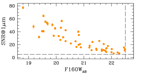
In order to perform a homogeneous selection of the targets based on stellar mass, we use the same photometric data in all four FIGS pointings, available from the 3D-HST survey (Skelton et al., 2014). We select all targets within a redshift range 0.5 $<z<$ 2.5 and derive stellar masses using the fluxes in F606W, F775W, F850LP (from HST/ACS), F125W, F140W, F160W (from HST/WFC3), as well as K_s (from Subaru/MOIRCS in the North and VLT/ISAAC in the South), and Spitzer/IRAC 3.6$\mu$m fluxes. We only select sources with F160W $<$ 22.5 AB, as the grism data become very noisy at fainter magnitudes. Note that in this paper we perform spectral fitting on slitless grism data corresponding to individual galaxies, rather than relying on stacking large numbers of galaxies at low SNR (as in the 3D-HST survey, Fumagalli et al., 2016). As an example, the WFC3 exposure time calculator predicts a S/N around 5 per resolution element for an unresolved F160W=22.5 AB source in the G102 grism, with the typical (100ks) exposures of the FIGS fields. Fig. 1 shows the observed SNR in the G102 grism data (evaluated at $\lambda=1\mu$m) as a function of F160W total magnitude.

Figure 2: Comparison of our starting set of stellar masses with the 3D-HST masses (Skelton et al., 2014, labelled Skel14), or the CANDELS estimates (Santini et al., 2015, labelled Sant15), adopting the same (Chabrier) IMF. The scatter, given as one half of the difference between the 75% and the 25% of the distribution is 0.15 in both cases. The panel on the right shows the distribution of mass offsets.

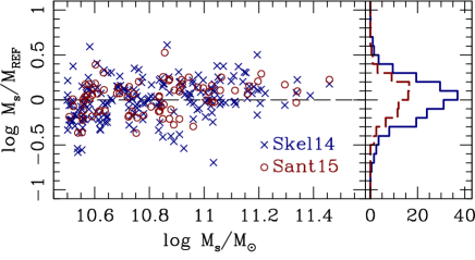
The stellar masses are derived from a comparison between the observed photometric fluxes and a set of composite populations assembled from a base set of 3 $\times$ 4 simple stellar populations (SSPs) from the models of Bruzual & Charlot (2003) for a Chabrier (2003) initial mass function (IMF). The set comprises three metallicities ([Z/H]={-0.5,0.0,+0.3}) and four ages (logarithmically spaced between 0.1 Gyr and the age of the Universe at the redshift of each galaxy). An ensemble modelling the underlying probability distribution function is created with a Monte Carlo Markov Chain code based on the Foreman-Mackey et al. (2013) emcee sampler, where the free parameters are the weights of each of the 12 SSPs, along with a reddening parameter, E(B$-$V), applied as a foreground screen, following the standard Milky Way extinction law (Cardelli et al., 1989). We note that the uncertainties in the derivation of stellar masses are significantly smaller than those related to the other population parameters (such as age and metallicity) at a fixed IMF (see, e.g. Ferreras, Saha & Burles, 2008). Moreover, at this stage we want to make sure we select all massive galaxies within the adopted redshift range and flux limit. Fig. 2 shows a comparison of our working stellar masses with the estimates of 3D-HST from Skelton et al. (2014), and those from Santini et al. (2015) in the CANDELS survey. We restrict the comparison to our mass threshold, $\log$M_s/M${}_{\odot}\geq$10.5, although the agreement is equally good down to stellar masses $\log$M_s/M_⊙=9.5. The SIQR statistic comparing our mass estimates with those from these published studies is 0.15 dex (3D-HST) and 0.14 (CANDELS). Although the derivation of stellar masses is not critical for our purposes at this stage, Fig. 2 suggests a potential systematic trend (comparable to the observed scatter), which can be attributed to the use of specific functional forms for the star formation rates.

Figure 3: Distribution of stellar mass with respect to redshift (left) and F160W magnitude (right). The filled dots are all galaxies detected in FIGS, whereas the open dots show our working sample of galaxies with good quality FIGS + PEARS grism data for spectral fitting constraints.

Figure 4: Postage stamps of the 51 galaxies in our FIGS sample. Each stamp is a WFC3/F160W image from CANDELS (Grogin et al., 2011; Koekemoer et al., 2011), covering a $16^{\prime\prime}\times 16^{\prime\prime}$ area. The stamps are labelled with the field: (0=GN1, 1=GN2, 2=GS1), and the corresponding ID. A stamp of the additional galaxy in this sample, FW4871, can be seen in Fig. 2 of Ferreras et al. (2012).

The starting sample of massive galaxies is then matched to the catalogue of FIGS WFC3/G102 spectra, as well as to the catalogue of slitless spectra from the PEARS ACS/G800L survey (ID 10530, PI Malhotra, e.g. Ferreras et al. 2009). The WFC3/G102 grism covers the 0.8-1.15 $\mu$m spectral window at a resolution of R=210; and the ACS/G800L (WFC) observations extend over the interval 0.55–1.05 $\mu$m at R=100. When available, we add WFC3/G141 grism data analyzed as part of programme AR 13266 (PI Ryan). This grism provides a spectral coverage 1.075–1.7 $\mu$m at resolution R=130. From this starting sample we retain only those galaxies for which both PEARS (G800L) and FIGS (G102) spectra are available. We note that only three of the four FIGS pointings (GN1, GN2 and GS1; see Table 1) overlap with PEARS data. The FIGS GS2 pointing targets a parallel CDFS field (HUDF-Par 2), not included in the ACS grism programme.

For each target and grism dataset, we correct the individual spectra – taken at a specific telescope roll angle – for contamination from nearby sources as computed in Pirzkal et al. (2017). We combine the corrected spectra (excluding, in very few cases, those that deviate more than 3 $\sigma$ from the average), and compute the uncertainty associated with the mean spectrum by propagating the errors of the individual spectra. The average PEARS and FIGS spectra of each galaxy are subsequently combined by scaling, in flux, the PEARS spectrum to the FIGS one within their overlapping spectral range, making sure to avoid data at the edges, where the instrument sensitivity drops and the flux calibration is not reliable. In the overlapping spectral region, the FIGS/G102 mean spectrum is interpolated to the dispersion of the scaled mean PEARS/G800L data. The two spectra are averaged and their errors propagated. The same procedure applies when combining the mean FIGS/G102 and G141 spectra. In this case the mean, G102 spectrum is interpolated to the dispersion of the lower-resolution G141 spectrum. Moreover, the G141 data are scaled to match the flux of G102. We exclude from this processing all galaxies whose spectra (either PEARS or FIGS) are truncated because the source is located at the edge of the field of view.

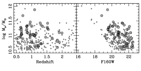
Table 1 summarizes the source selection. Fig. 3 shows the starting sample, as grey dots, and the final sample of galaxies with good PEARS and FIGS data for the spectral analysis presented below. Clearly, the combination of PEARS and FIGS data provide a wide coverage for the spectral fitting analysis, which in turn allows us to better constrain the star formation histories of massive galaxies in the rest-frame optical window. We cross-correlated the sample with the X-ray 2 Ms catalogues in the CDFN (Alexander et al., 2003) and CDFS (Luo et al., 2008), and only found three sources with a hard X ray detection (in the 2-8 keV band), namely galaxies 2144 and 2502 in GN1 and galaxy 980 in GS1, with X-ray fluxes L${}_{X}=\{0.01,0.02,0.35\}\times 10^{44}$erg s^-1, respectively. Given the low luminosity of these sources, we do not expect the rest-frame optical fluxes to be contaminated by AGN emission.

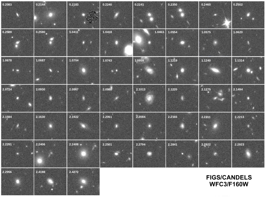
Fig. 4 shows the WFC3/F160W images of the final set of 51 galaxies from CANDELS (Grogin et al., 2011; Koekemoer et al., 2011). We note that the FIGS fields GN1 and GN2 are covered by the CANDELS GN05 GOODS-N pointing, and that GS1 is fully covered by the CANDELS GSD01 GOODS-S pointing. In the appendix, Table 5 shows the general details of the sample, including visual morphology, stellar coordinates, redshift and F160W magnitude, as well as stellar mass and rest-frame U$-$V and V$-$J colours (derived from the spectral analysis, see below). The morphology estimate is split into early-types (E) and late-types (L), and follows Huertas-Company et al. (2015), who train a set of convolutional neural networks on the results from a visual classification in the $H$ band (Kartaltepe et al., 2015) to produce a catalogue of “visual-like” classifications in the five CANDELS fields. We use their spheroid fraction parameter to split our sample into early- ($f_{\rm Sph}\geq 0.5$) and late-types ($f_{\rm Sph}<0.5$). Next to the morphological type (col. 3 of Table 5) we include the quiescence (Q) vs star-formation (S) flag based on the standard analysis on a colour-colour diagram, as presented in §4. Note that in addition to the 51 galaxies from the combined PEARS+FIGS sample, we include the spectrum of massive galaxy FW4871 (presented in Ferreras et al., 2012), also produced from a combination of ACS and WFC3 grism data.

Figure 5: Examples of the full spectral fitting results, combining the ACS and WFC3 grism data. We show galaxies FW4871 (z=1.893, left) and GN1/2144 (z=0.943, right). The slitless grism data are shown as green dots, and the best fit model is given by the solid line. For reference, we include the broadband photometry as orange triangles, with the horizontal error bars representing the FWHM of the bandpasses. The insets show the fractional contribution by mass of the six base models, labelled with respect to their average stellar age. The extracted star formation history reveals a younger population in 4871 (average age of $\sim$1 Gyr) with respect to 2144 ($\sim$2 Gyr), as reflected by the prominent Balmer absorption features (see §3 for details). The rest of the spectral fits are shown in the appendix.

2.1 Surface brightness fits and colour gradients

In addition to the low-resolution grism spectra, we perform a surface brightness analysis, applying Galfit (Peng et al., 2002) to the CANDELS WFC3 images in F125W and F160W (Koekemoer et al., 2011). We consider a single Sérsic profile, and the sizes are quoted as the circularized half-light radii, i.e. $R_{e}\equiv\sqrt{a_{e}b_{e}}$, where $a_{e}$ and $b_{e}$ are the semi-major and semi-minor axes, respectively, engulfing half of the total light. An image of the point spread function for each pointing and field is created by median stacking a number of stars in the CANDELS GN05 and GSD01 fields. We inspected visually the fits, making sure there were no significant residuals. Moreover, we compared our results in the F160W band with the surface brightness fits presented in van der Wel et al. (2012), and find a difference in the Sérsic index of $\Delta n_{S}\equiv n_{\rm S,FIGS}-n_{\rm S,vdWel}=-0.18\pm 1.04$ and in the effective radius of $\Delta R_{e}\equiv R_{\rm e,FIGS}-R_{\rm e,vdWel}=0.05\pm 0.18$ arcsec. We note that the CANDELS radii are quoted as the half-light semi-major axis, so this comparison involves the raw Galfit sizes (also given as the semi-major axis).

The analytic surface brightness profiles, using the best fit parameters from each band, are combined to create a $C\equiv$F125W$-$F160W colour profile, from which we derive, via a standard least squares linear fit, a slope of the (linear) radial gradient: $\nabla_{C}\equiv\Delta C/\Delta\log R$. Table 6, in the appendix, shows the results of the F160W surface brightness fits and colour profiles. As a test, we compared the visual morphological classification (from col. 3 in Table 5) with the Sérsic index (from col. 3 in Table 6), finding an average value of $n_{S}$=3.4$\pm$2.6 for the early-types, and $n_{S}$=1.3$\pm$0.7 for the late-types. There does not seem to be a similar segregation in the colour gradient with respect to visual morphology (average gradients of $\nabla_{C}=-$0.07$\pm$0.16 and $-$0.04$\pm$0.27 for the early- and late-types, respectively), but a potential variation if the sample is segregated with respect to the Sérsic index (average gradients of $\nabla_{C}=+$0.03$\pm$0.05 and $-$0.11$\pm$0.24 for n${}_{S}>$2.5 and n${}_{S}\leq$2.5, respectively).

3 Spectral fitting

The fitting procedure involves two stages. In the first stage we perform an initial fit of the spectra using simple stellar populations (SSPs) from the synthetic models of Bruzual & Charlot (2003) for a Chabrier (2003) initial mass function (IMF). Although the use of SSPs is rather simplistic, the high level of correlation of any spectra involving unresolved populations allows us to assess whether a good fit is possible, and we also use this initial fit to mask bad data, or strong emission lines, by applying a 4 $\sigma$ clip. Moreover, we test the effective resolution of the spectra and the spectral fitting range. We take into account the fiducial resolution of the grisms – namely R=100 @$\lambda=0.8\,\mu$m for ACS/WFC/G800L; R=210 @$\lambda=1\,\mu$m for WFC3/G102, and R=130 @$\lambda=1.4\,\mu$m for WFC3/G141, all valid for an unresolved source. In slitless spectroscopy, the effective resolution depends on both the actual resolution of the dispersion element, and the surface brightness profile of the galaxy along the dispersion direction, since the source acts as a slit. The spectral resolution of the grisms quoted above correspond to an unresolved object, whereas an extended source will produce significantly lower values. We address this issue by taking into account the Sérsic surface brightness profiles presented in §§ 2.1. These profiles are convolved along the dispersion direction with the synthetic data, in order to obtain spectra with the same effective resolution as the observed data. This is done on a galaxy-by-galaxy basis. Once the fit is satisfactory, the code creates a set of five “base models” for each galaxy, with a constant star formation rate defined within the age intervals as follows:

Figure 6: Example of the parameter fits corresponding to galaxy FW4871 (z=1.89, stellar mass $7.95\times 10^{11}$M_⊙). A set of panels shows the 2D marginalised distribution of the parameters (see text for details). The spectral fit is shown in Fig. 5 (left panel).

• Base Model 1: $\log t/{\rm Gyr}\in[-2,-1]$

• Base Model 2: $\log t/{\rm Gyr}\in[-1,-0.3]$

• Base Model 3: $\log t/{\rm Gyr}\in[-0.3,0.0]$

• Base Model 4: $\log t/{\rm Gyr}\in[0.0,0.3]$

• Base Model 5: $\log t/{\rm Gyr}\in[0.3,lt_{\rm MAX}]$

• Base Model 6: $\log t/{\rm Gyr}\in[0.3,lt_{\rm MAX}]$

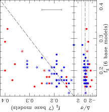
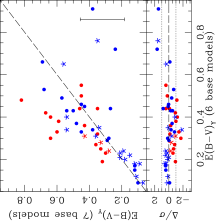
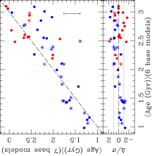
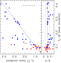
where $lt_{\rm MAX}$ is the log₁₀ of the age of the Universe at the redshift of the galaxy, i.e. corresponding to the oldest possible age. These base models have the same metallicity as the best-fit value obtained during the first fitting stage. Note the sixth base model has the same age distribution as BM5, but at a metallicity lower than the best fit value by $-0.3$ dex. Base Model 6 thus represents an old, metal-poor component expected in formation histories with a low star formation efficiency. Although this component should not dominate the budget in massive galaxies (e.g. Ferreras & Silk, 2000), we include this potential contribution as a free parameter. We note that the choice of six base models may seem rather arbitrary. However, we point the reader to Sec. 4.2, where PCA suggests most of the variance in the data can be encoded into $\sim$4-5 components. Our use of five time components plus an additional old and metal poor one is thus a good compromise to constrain the stellar populations in these galaxies. In appendix C, we compare our results with a new set of runs where seven base models are considered, finding consistent constraints.

Figure 7: Rest-frame colour-colour diagram, showing the standard regions defining quiescent and star forming galaxies, following Williams et al. (2009). The solid (dashed) line corresponds to 1$<$z$<$2 (0.5$<$z$<$1). Our sample is split with respect to visual morphology, with early-types shown as filled dots and late-types as star symbols. The sample is colour coded, with red (blue) galaxies representing quiescent (star-forming) galaxies, as shown in Fig. 9. The open triangle represents galaxy FW4871. A characteristic error bar, at the 1 $\sigma$ level, is shown in the top-left corner. For reference, two tracks from the population synthesis models of Bruzual & Charlot (2003) are shown, SSP for a quiescent population, and CST for constant star formation (see text for details). The arrow is the $A_{V}=1$ dust attenuation vector.

The second stage of the fitting procedure uses the six base models to perform linear superpositions – exploring a wide range of complex star formation histories – and including the presence of dust. We use the standard extinction law of Cardelli et al. (1989) and consider two independent reddening components – each parametrised by a standard colour excess E(B$-$V). One component is expected to originate from star-forming regions, and is only applied to the two youngest components (BM 1 and 2). We note that the typical timescales for the dispersion of dust clouds in star forming regions is significantly shorter than the age of BM2 (see, e.g. Charlot & Fall, 2000). However, we are targeting the whole stellar distribution of these galaxies as one composite population, and our simple phenomenological model aims at assessing whether the populations from the younger stars in a potential post-starbursting system, are significantly more affected by dust than the general stellar component. A second dust parameter traces the diffuse distribution and affects the whole spectrum. This seven parameter model is fitted using an implementation of the Python MCMC sampler emcee (Foreman-Mackey et al., 2013). The models and data are normalized in the observer frame $\lambda\sim 0.9-1.0\,\mu$m spectral window.

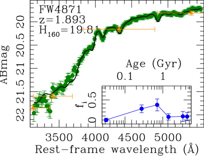
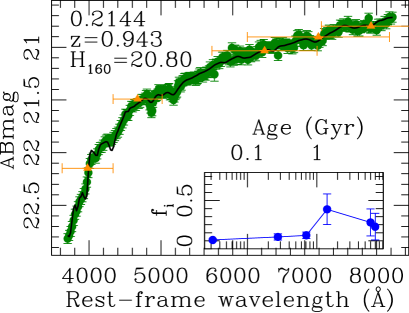
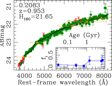
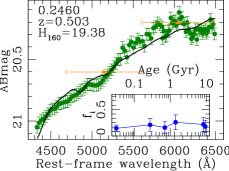
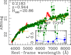
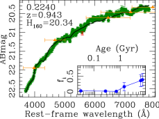
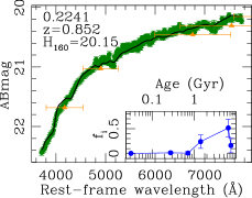
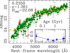
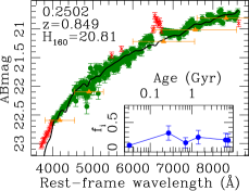
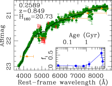
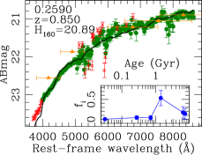
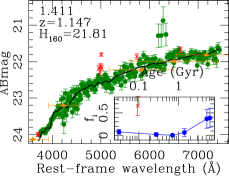
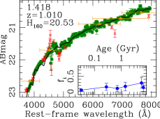
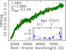
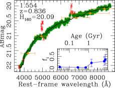
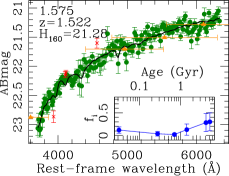
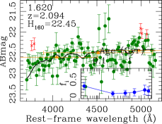
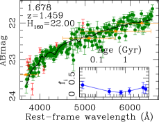
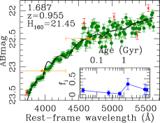
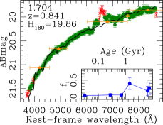
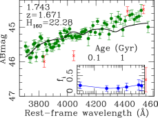
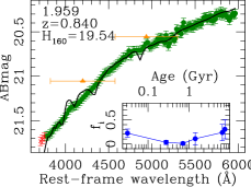
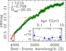
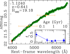
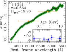
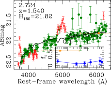
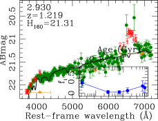
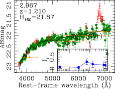
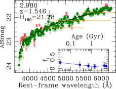
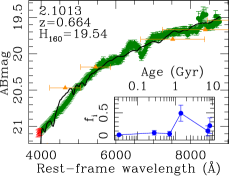
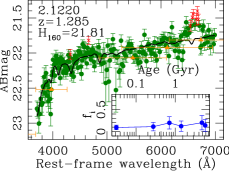
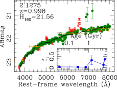
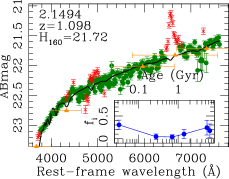
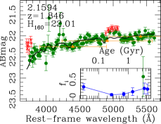
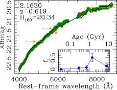
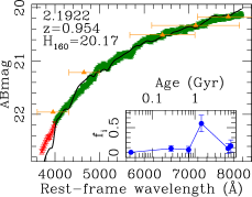
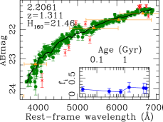
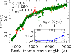
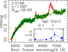
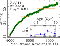
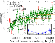
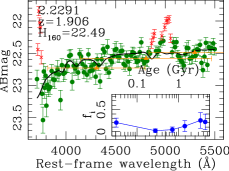
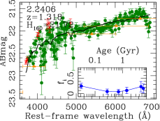
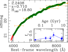
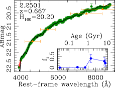
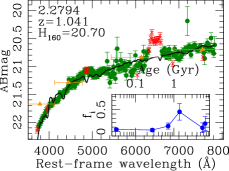
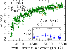
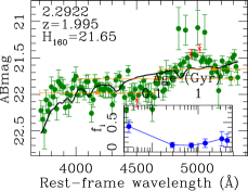
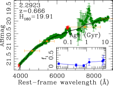
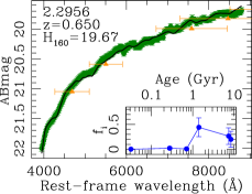
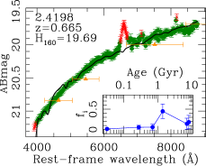
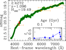
Fig. 5 illustrates two examples regarding the fitting results. The panel on the left shows galaxy FW4871, whose WFC3 NIR spectra in G102 and G141 were obtained during the WFC3 ERS programme (Windhorst et al., 2011), and was combined with the optical ACS/G800L data (Ferreras et al., 2012). This source is a z=1.89 galaxy, identified as a typical near-quiescent, compact massive galaxy, potentially a progenitor of the cores found in massive early-type galaxies at low redshift. The panel on the right shows GN1/2144, another massive galaxy, this time from the combined FIGS+PEARS data. Each panel shows the observed fluxes as filled green circles with error bars, along with the best fit model (solid line). Orange triangles give, for reference, the fluxes in broadband filters covering the same spectral window, from the available photometry in the {F606W, F775W, F850LP, F125W, F140W, F160W} passbands. The inset in each panel shows the weight, along with error bars of each of the six base models with respect to the age of each one, giving an estimate of the star formation history. For ease of visualization, Base Model 6 (that has the same age as BM5) is displaced by $+$1 Gyr. Similar plots for the whole sample are shown in the appendix.

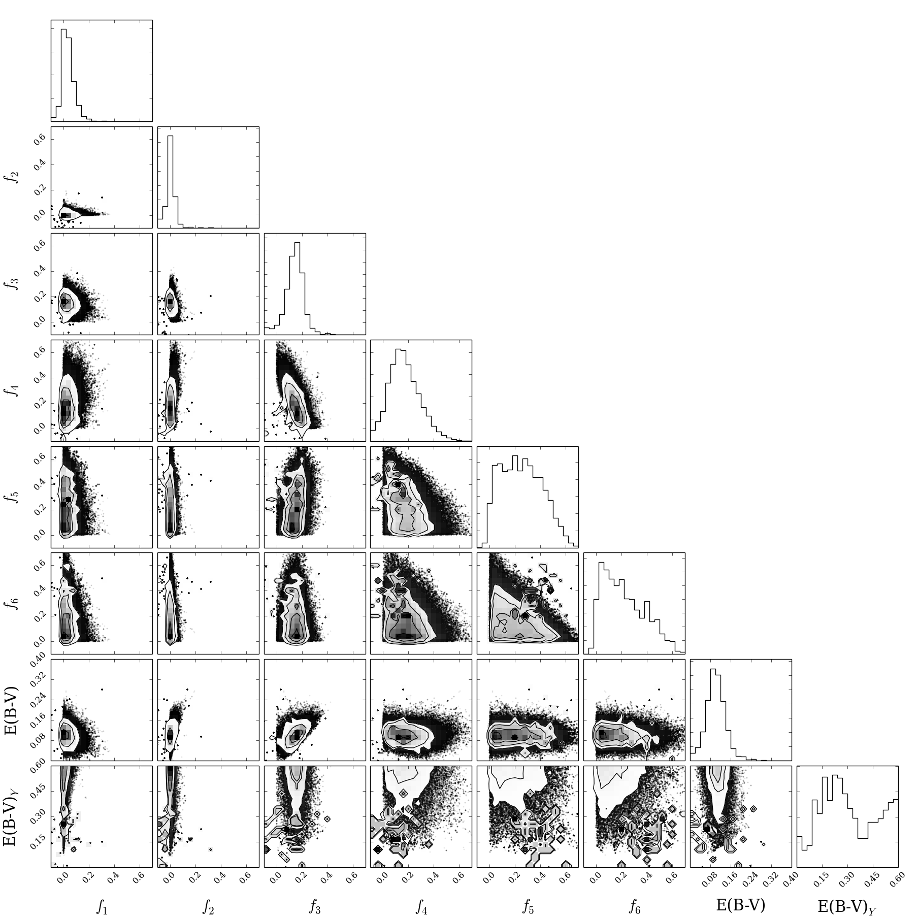
The confidence levels of the fitting parameters of FW4871 are shown, for reference, in Fig. 6, with contours at the 1, 2, and 3 $\sigma$ levels. For a comparison between this free form, component-based fitting and a more standard approach with exponentially decaying (or constant-plus-truncation) star formation histories, we refer the interested reader to Ferreras et al. (2012), where a detailed comparison is made. As a reference, we note that the average age quoted here for FW4871 ($1.18\pm 0.19$ Gyr) is compatible with those derived from such generic functional forms: $0.72\pm 0.10$ Gyr for an exponentially decaying SFH, and $1.44\pm 0.20$ Gyr for a constant SFH, both derived from the spectrum extracted within the inner $0^{\prime\prime}.64$ region of FW4871 (all quoted at the 1 $\sigma$ level). As discussed in detail in Ferreras et al. (2012), we emphasize that the use of exponentially decaying functions can lead to significant biases in the estimates of stellar age and formation timescale (see also Simha et al., 2014).

From the best fit models, we derive a number of properties, including the best-fit metallicity, the average age, weighted according to the mass fractions of each base model: ${f_{1},\cdots f_{6}}$, the age of the oldest 10% stars ($t_{10}$), and a parameter that characterizes the width of the age distribution ($\Delta t$), defined as the difference between the average age and $t_{90}$, where $t_{90}$ is the age of the youngest 10% fraction (by mass) of the stellar component. We use the subindex $90$ here as these stars represent a cumulative fraction at the 90% level (and to distinguish this parameter from $t_{10}$, as defined above). The fitting parameters are listed in Table 5 and 7, including error bars at the 1 $\sigma$ level. The uncertainties are derived from the MCMC sampling, taking the last 1000 points from the chains. The parameter $t_{10}$ serves as a proxy of the formation time, with higher values implying earlier formation. For instance, galaxy GN1/2083 has $t_{10}=2.9$ Gyr, meaning that the oldest 10% of its stellar populations have ages older than 2.9 Gyr. At the redshift of this galaxy (z=0.953), this implies a formation redshift around $z_{\rm FOR}\lower 2.15277pt\hbox{$\;\buildrel>\over{\sim}\;$}2.1$. We also define f${}_{Y}\equiv$f₁+f₂ as the stellar mass fraction in the youngest components (BM1 and BM2); and f${}_{Z}\equiv$f₆ as the mass fraction in low-metallicity stars (i.e. BM6).

Figure 8: Mass vs size relation of our sample of massive galaxies. The symbol and colour coding is the same as in Fig. 7, with red (blue) symbols representing quiescent (star-forming) galaxies and filled dots (stars) coding the visual morphology as early-types (late-types). The local relation from Shen et al. (2003) for early-type galaxies is given by the solid line, with the dashed lines marking a $\pm 0.3$ dex region about this fit. The compact galaxies are hereafter represented by the larger open circles.

4 Population trends

Figure 9: The age-related parameters are plotted with respect to stellar mass. The sample is split between quiescent (red) and star-forming galaxies (blue), and between early-types (circles) and late-types (stars), as defined in Fig. 7. In each panel we show a linear fit to each subsample. Typical error bars are given at the 1 $\sigma$ level. Galaxies that appear more compact than the local mass-size relation (see Fig. 8) include an open circle. The dotted grey line in the top-right panel shows the expected trend in relative age (age/$t_{U}$) for a population formed in a single burst at z_FOR=3.

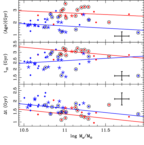
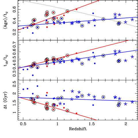
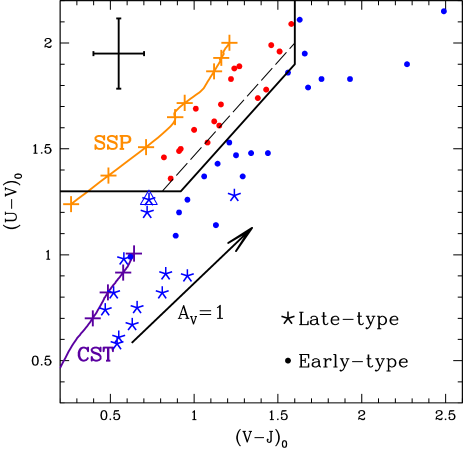
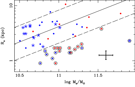
Fig. 7 shows the rest-frame $(U-V)_{0}$ and $(V-J)_{0}$ colours, derived from the best-fit models. This colour-colour diagram has become a standard tool when separating galaxy samples between quiescent and star-forming systems (e.g. Williams et al., 2009). The symbols split the sample into late- and early-type galaxies, following our visual classification, and we follow the colour criterion of Williams et al. (2009) to define quiescent and star-forming galaxies. Hereafter, the figures show these two subsamples in red and blue, respectively. Note the strong correlation between the photometric selection and the morphological one, where most star forming galaxies – especially towards the bottom-left part of the diagram – display a late-type morphology (star symbols) and all quiescent galaxies have an early-type morphology (solid circles). In addition, galaxy FW4871 is shown as an open triangle. This galaxy is at the boundary between star-forming and quiescent behaviour, as expected since its spectrum shows strong Balmer absorption on a quiescent continuum (see Fig. 5, left panel), a typical feature of post-starburst galaxies (Ferreras et al., 2012). The fact that most of the early-type galaxies classified as star-forming appear in the transition region suggests a similar type of post-starburst behaviour. However, we should warn that the morphological classification may be limited by the effect of dust. For reference, two tracks from the population synthesis models of Bruzual & Charlot (2003) are shown: the orange (labelled SSP) corresponds to a quiescent population with ages marked by the crosses – from left to right: {0.5, 0.75, 1, 1.5, 1.75, 2, 3, 4, 5} Gyr. The purple line (labelled CST) is a constant star formation history, with crosses marking the ages (also from left to right) {2, 3, 4, 5} Gyr. The dust vector for a Cardelli et al. (1989) attenuation law with $A_{V}=1$ is shown as an arrow. The classification based on either star formation activity or visual morphology is also presented, with the same symbols and colour coding, on a mass vs size plane in Fig. 8. For reference, the local relation observed in early-type galaxies (from Shen et al., 2003) is shown as a solid line, including a $\pm 0.3$ dex region accounting for the scatter, as dashed lines. A significant fraction of our sample comprises compact systems, marked with open circles. We will show in the figures below the same identification to assess whether the compact galaxies in our sample present any differences regarding their stellar populations. We emphasize that our definition of the compactness criterion is rather simplistic, as we only use the local relation of early-type galaxies and a 0.3 dex offset. This work does not aim at a detailed analysis of compact galaxies, but is meant, instead, to roughly assess whether compact galaxies display significant differences with respect to the general sample of massive galaxies.

…

Table 2: Linear regression to the results shown in Figs. 9 and 10, with respect to stellar mass. The model for parameter $\pi$ is $\pi=a\log M_{11}+b$, where $M_{11}$ is the stellar mass in units of $10^{11}$M_⊙ and $\pi$ corresponds to the following: average age, $t_{10}$, $\Delta t$, $f_{Y}$, $f_{Z}$, or metallicity. Col. 1 identifies the parameter fit, col. 2 identifies the sample considered: Q for quiescent and SF for star-forming. Cols. 3 and 4 give the slope ($a$) and intercept ($b$) at $10^{11}$M_⊙, respectively. Col. 5 is the linear correlation coefficient. The error bars, quoted at the 1 $\sigma$ level, take into account the individual uncertainties of the measurements.

$\pi$	Ty	$a$	$b$	$\rho_{xy}$
(1)	(2)	(3)	(4)	(5)
$\langle{\rm Age}\rangle/t_{U}$	Q	$-0.02\pm 0.10$	$0.44\pm 0.03$	$+0.08\pm 0.12$
	SF	$-0.00\pm 0.04$	$0.37\pm 0.01$	$-0.03\pm 0.14$
$t_{10}/t_{U}$	Q	$+0.12\pm 0.05$	$0.48\pm 0.02$	$+0.11\pm 0.13$
	SF	$+0.02\pm 0.04$	$0.47\pm 0.01$	$-0.05\pm 0.15$
$\Delta t$	Q	$-0.41\pm 0.26$	$1.38\pm 0.07$	$-0.17\pm 0.16$
	SF	$-0.40\pm 0.16$	$1.65\pm 0.05$	$-0.24\pm 0.15$
$f_{Y}$	Q	$-0.01\pm 0.04$	$0.06\pm 0.01$	$-0.09\pm 0.16$
	SF	$+0.01\pm 0.09$	$0.22\pm 0.03$	$+0.01\pm 0.14$
$f_{Z}$	Q	$-0.06\pm 0.07$	$0.23\pm 0.02$	$-0.04\pm 0.19$
	SF	$-0.04\pm 0.03$	$0.18\pm 0.01$	$+0.01\pm 0.13$
[Z/H]	Q	$+0.11\pm 0.11$	$-0.10\pm 0.03$	$+0.19\pm 0.10$
	SF	$+0.17\pm 0.07$	$-0.08\pm 0.02$	$+0.23\pm 0.09$

Figure 10: This is the equivalent of Fig. 9 for the other spectral fitting parameters, from top to bottom: fraction of mass in young stars (f_Y), fraction of mass in low-metallicity stars (f_Z) and average metallicity ([Z/H]), The sample is split between quiescent (red solid) and star-forming galaxies (blue open), as defined in Fig. 7. In each panel we show a linear fit to each subsample. Typical error bars are given at the 1 $\sigma$ level. Galaxies that appear more compact than the local mass-size relation (see Fig. 8) include an open circle.

…

Table 3: Equivalent of Table 2 using redshift to perform the correlation analysis. Linear regression to the results shown in Figs. 9 and 10. The model for parameter $\pi$ is $\pi=a(z-1)+b$, where $\pi$ corresponds to the following: average age, $t_{10}$, $\Delta t$, $f_{Y}$, $f_{Z}$, or metallicity. Col. 1 identifies the parameter fit, col. 2 identifies the sample considered: Q for quiescent and SF for star-forming. Cols. 3 and 4 give the slope ($a$) and intercept ($b$) at z=0, respectively. Col. 5 is the linear correlation coefficient. The error bars, quoted at the 1 $\sigma$ level, take into account the individual uncertainties of the measurements.

$\pi$	Ty	$a$	$b$	$\rho_{xy}$
(1)	(2)	(3)	(4)	(5)
$\langle{\rm Age}\rangle/t_{U}$	Q	$+0.44\pm 0.11$	$0.49\pm 0.10$	$+0.57\pm 0.11$
	SF	$+0.09\pm 0.02$	$0.36\pm 0.03$	$+0.41\pm 0.11$
$t_{10}/t_{U}$	Q	$+0.24\pm 0.03$	$0.51\pm 0.02$	$+0.72\pm 0.10$
	SF	$+0.14\pm 0.02$	$0.46\pm 0.02$	$+0.58\pm 0.14$
$\Delta t$	Q	$-1.06\pm 0.20$	$1.21\pm 0.18$	$-0.58\pm 0.11$
	SF	$-0.12\pm 0.10$	$1.73\pm 0.12$	$-0.28\pm 0.14$
$f_{Y}$	Q	$+0.01\pm 0.04$	$0.05\pm 0.03$	$-0.03\pm 0.16$
	SF	$+0.13\pm 0.05$	$0.21\pm 0.06$	$+0.19\pm 0.11$
$f_{Z}$	Q	$+0.19\pm 0.11$	$0.25\pm 0.10$	$+0.30\pm 0.20$
	SF	$-0.01\pm 0.02$	$0.19\pm 0.03$	$+0.00\pm 0.14$
[Z/H]	Q	$+0.02\pm 0.15$	$-0.08\pm 0.13$	$-0.01\pm 0.19$
	SF	$-0.04\pm 0.04$	$-0.10\pm 0.05$	$-0.10\pm 0.15$

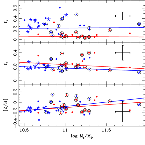
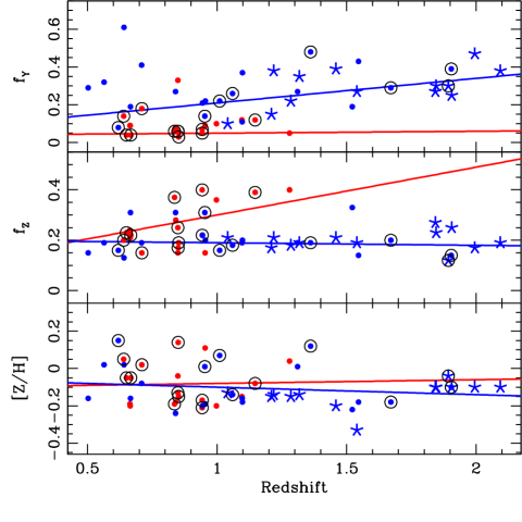
The trends of the population parameters with stellar mass are presented in Figs. 9 and 10, following the same notation regarding symbol shape and colour as in Fig. 7. We note that the redshift range covered by our sample maps into a large interval of cosmic time, between 3.2 and 8.4 Gyr (quoted as the age of the Universe at z=2 and z=0.5, respectively). We emphasize that this paper is not meant to look for one-to-one evolutionary paths of massive galaxies. At the redshifts covered, these galaxies could have a wide and disjoint range of potential progenitors (e.g. Choi et al., 2014). We want to study instead, the general properties of massive galaxies over a period that encompasses the peak of galaxy formation. These properties reflect the complex mixture of evolutionary trends. To mitigate the large redshift range covered, the age-related population parameters that are expected to vary with lookback time are factored by the age of the Universe at the redshift of the galaxy ($t_{U}$). Therefore, the average stellar age is replaced by the relative age, defined as the fraction age/$t_{U}$. For instance, in a monolithic formation scenario, the old quiescent populations will vary with redshift similarly to the age of the Universe: a galaxy formed instantaneously at z_FOR=3 will have an age/$t_{U}$ parameter varying from 0.35 at z=2 to 0.75 at z=0.5 (see dotted line on the top-right panel of Fig. 9). More recent (earlier) formation redshifts will result in a wider (narrower) range of relative ages. Variations of this parameter will therefore suggest differences in the stellar age distribution. Figs. 9 and 10 show the parameters extracted from our methodology as a function of stellar mass (left) and redshift (right).

Figure 11: Radial colour gradients (defined as $\nabla_{C}\equiv\Delta C/\Delta\log R$, where $C\equiv$F125W–F160W), plotted as a function of (top from left to right): redshift, stellar mass, effective radius in physical units, and Sérsic index; (bottom, from left to right): average stellar age, and $t_{10}$, both relative to the age of the Universe, $\Delta t$, and mass fraction in young stars The symbols follow the previous figures, with red/blue representing quiescent/star forming populations and dot/star plotting early-/late-types, respectively. Typical error bars are shown at the 1 $\sigma$ level. Galaxies that appear more compact than the local mass-size relation (see Fig. 8) include an open circle.

The results from a linear regression analysis of the data presented in these two figures are shown in Table 2 (with respect to the logarithm of stellar mass) and Table 3 (with respect to redshift), giving the slope, the best fit value at a fiducial point ($10^{11}$M_⊙ in mass and z=1 in redshift), as well as the correlation coefficient $\rho_{xy}$. The errors are quoted at the 1 $\sigma$ level, as derived by the SciPy Orthogonal Distance Regression package (ODR, Boggs & Rogers, 1990). The errors in the correlation coefficient – derived via the SciPy stats.linregress package – are estimated from a Monte Carlo sampling of 100 realizations produced by adding Gaussian noise as expected from the parameter uncertainties. The analysis takes into account the uncertainties in the individual data points, as quoted in the pertinent tables. The solid lines in Figs. 9 and 10 represent the best fits. Note the typical mass-related trend such that quiescent galaxies are more massive than star-forming systems. Moreover, at fixed stellar mass, the age/$t_{U}$ ratio is younger in the latter subset, supporting the use of the UVJ colour-colour diagram to classify quiescent and star-forming galaxies (Labbé et al., 2005). The lack of quiescent galaxies at z$\;\buildrel>\over{\sim}\;$1.5 cannot be explained by the flux limit of our sample: an SSP with solar metallicity, formed at redshift z_FOR=5 (using the models of Bruzual & Charlot, 2003) has F160W=21.5 at z=1.5 or 22.1 at z=2.0, within the range of our observations (see Fig. 1).

Figure 12: Comparison between the model parameters derived from the fiducial set of BC03 models (Bruzual & Charlot, 2003, horizontal axes) and those extracted from the MIUSCAT models (Vazdekis et al., 2012, vertical axes). For reference, a 1:1 straight line is included in all panels, as well as a typical error bar. The notation of the symbols follow the previous figures. Timescales are shown in Gyr.

Neither average age/$t_{U}$ nor $t_{10}$/$t_{U}$ give robust correlations with stellar mass. The width of the age distribution ($\Delta t$, bottom panel of Fig. 9, left) shows a weak level of correlation in the star-forming subsample, with a decreasing trend with stellar mass. The quiescent sample appear to follow a similar decreasing trend, but the $\rho_{xy}$ coefficient (col. 5 of Table 2) is, however, compatible with no correlation, mostly due to the limited mass range of the quiescent subsample. At fixed mass, the star-forming galaxies have slightly longer values of $\Delta t$ than the quiescent galaxies. We emphasize that this sample is restricted to the massive end, where age-mass trends tend to level out (see Gallazzi et al. 2005 for the mass-age trend at low redshift, or Gallazzi et al. 2014 at z$\;\buildrel<\over{\sim}\;$0.7). With respect to redshift, significantly increasing trends are found in age/$t_{U}$ and $t_{10}$/$t_{U}$. The top-right panel of Fig. 9 shows, as a dotted grey line, the expected evolution of the relative age for a single burst population formed at z_FOR=3 (earlier redshifts will shift the curve to higher values). Such trend – posited by the traditional monolithic collapse scenario – is at odds with the observations, that suggest the opposite behaviour, namely as time evolves, younger populations are being incorporated into massive galaxies, decreasing their relative age. The same trend is obtained in the $t_{10}$/$t_{U}$ parameter, reinforcing the idea of a continuous contribution of additional populations. In such a scenario, the parameter $\Delta t$ should also be expected to produce larger values (more extended age distributions) at lower redshift, as shown in the bottom-right panel of Fig. 9. A similar trend is found in a large sample ($\sim$8,500) of quiescent galaxies from the ALHAMBRA medium band survey (Díaz-García et al., 2018), and our results are consistent with the spectral fitting of stacked SDSS data presented by Choi et al. (2014).

A significant difference is unsurprisingly found in the distribution of the fraction in young stars (f_Y, top panel of Fig. 10, left) between the quiescent and the star forming sample. No trend is noted with stellar mass in either subsample, but a large scatter is found in star-forming galaxies. The mass fraction in low-metallicity stars (f_Z, middle panel) does not show a significant difference between these two sets, giving an average around 20% of the total stellar mass content in stars with lower (by a factor of 2) metallicity with respect to the fiducial metallicity of the best-fit value. However, we note the error bars are larger for this parameter, and may be more affected by systematic effects (see §§4.1). Finally, the average metallicity (bottom panel) shows the usual positive correlation with mass, with a large scatter, although we note the model comparisons produce rather large uncertainties on the metallicity. As regards to the compact galaxy subsample (encircled galaxies in Figs. 9 and 10), no apparent difference is found, supporting the idea that the compactness criterion, at fixed mass and redshift, does not segregate the populations with respect to age (Trujillo, Ferreras, & de La Rosa, 2011). We emphasize this trend is not at odds with the age variations found on the mass-size plane at low redshift (Scott et al., 2017), as the analysis of these galaxies will be affected by the “second”, ex-situ step of growth within the 2-stage formation paradigm. Namely, the additional material incorporated via mergers, will potentially introduce a systematic trend making extended galaxies, at fixed mass, younger. Regarding the redshift evolution of these parameters, the star forming subsample features an increasing trend of $f_{Y}$ with redshift, as expected from the higher star formation activity towards cosmic noon. The quiescent sample also features an intriguing increasing trend of $f_{Z}$ with redshift, but the scatter and the low number of galaxies makes this correlation rather weak. No redshift trend is found with respect to metallicity.

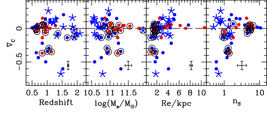
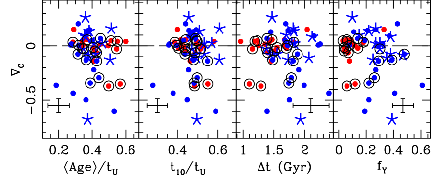
Fig. 11 plots the overall properties of the sample with respect to the F125W–F160W colour gradient, showing that most of the gradients are very small, especially in the quiescent, early-type dominated sample. Some of the star-forming galaxies with late-type morphology have slightly positive colour gradients (i.e. blue cores), an aspect that may reflect a central episode of star formation (see, e.g. Ferreras et al., 2009). However, the fraction in young stars ($f_{Y}$) appears not to correlate with colour gradients, so that our sample includes systems with star formation taking place either inside or outside of the core. It is also worth pointing out that the compact subsample (encircled symbols) have either flat or negative colour gradients (i.e. red cores), suggesting that the bulk of the stellar populations is located centrally, from a characteristic early, in-situ process.

4.1 Systematic effects related to population synthesis models

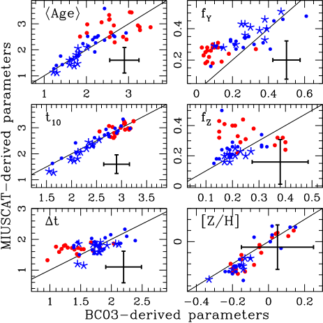
We explore the potential systematic effects on the derivation of population parameters by running the same method described above with base models created from the stellar population synthesis models MIUSCAT (Vazdekis et al., 2012), instead of Bruzual & Charlot (2003). These models use different sets of prescriptions, interpolation schemes and stellar libraries, so a comparison allows us to assess the robustness in our extracted parameters and the resulting error bars. We note that the only two differences in the methodology are: 1) the youngest base model (BM1), which originally comprises a constant star formation history between 10 and 100 Myr in our fiducial models is now restricted to the range 60–100 Myr as younger ages are not available in MIUSCAT; and 2) the stellar IMF used is Kroupa Universal (Kroupa, 2001), instead of Chabrier (2003) for the BC03 models.

Fig. 12 shows a comparison of the parameters extracted from these two different population synthesis models, showing an overall concordance, especially within error bars. We note that f_Z gives the most discrepant results, although the expected uncertainties are also rather large. The comparison also shows a higher mismatch at low f_Y and short $\Delta t$, but always compatible with the error bars. Therefore, we conclude that, as a “lowest-order” effect, the results found are resilient to variations among stellar population models.

Table 4: Principal Component Analysis: The table shows the first four principal components along with their projections along the stellar population parameters of this analysis. Col. 1 is the principal component rank, col. 2 gives the eigenvalue (as a percentage of total variance), and cols. 3-9 are the PC coefficients $\{c_{i}\}_{i=1}^{7}$, corresponding to the variables listed underneath.

Component	$\lambda$	$c_{1}$	$c_{2}$	$c_{3}$	$c_{4}$	$c_{5}$	$c_{6}$	$c_{7}$
	%	$\langle{\rm Age}\rangle/t_{U}$	$t_{10}/t_{U}$	$\Delta t$	$f_{Y}$	$f_{Z}$	E(B–V)	EY(B–V)
PC1	64.8	$-$0.18610	$-$0.09052	$+$0.91275	$+$0.29944	$-$0.11724	$+$0.10723	$-$0.09569
PC2	21.6	$+$0.08181	$+$0.16539	$-$0.03391	$+$0.04958	$+$0.00385	$-$0.37349	$-$0.90710
PC3	6.1	$-$0.07380	$+$0.03626	$-$0.35153	$+$0.89635	$-$0.14246	$+$0.21271	$-$0.02610
PC4	4.2	$-$0.57993	$-$0.45080	$-$0.19841	$-$0.25330	$-$0.46815	$+$0.27040	$-$0.25425

4.2 Looking for the driver of population variations with PCA

We can assess the distribution of the variance in the results with respect to the various population parameters by applying Principal Component Analysis (PCA) to the results. PCA consists of creating linear combinations of the model parameters for the sample so that these combinations (the principal components, PCs) are decorrelated. Moreover, these components are commonly sorted in decreasing order of variance, allowing us to determine which parameters are most responsible for the variance found in the sample. Table 4 shows the results for the first four principal components. Note that since the uncertainty in metallicity is rather large, we opted not to include this parameter in the analysis. Col. 2 gives the fractional contribution to the total variance, showing that these four components amount to over 96% of the total. The rest of the columns define the PCs as the coefficients corresponding to each of the model parameters. The first component (PC1, 64.8% of variance) is mostly dependent on $\Delta t$, and the second one (PC2, 21.6% of variance) mostly depends on the dust attenuation (both the diffuse component and the one only affecting young stars). The third component (PC3, 6.1%) is mainly dependent on the mass fraction in young stars, and PC4 is just shown to illustrate that at lower levels of variance, all model parameters contribute in a similar way (achieving some sort of noise level). Therefore, we can say that our analysis mostly discriminates with respect to the width of the age distribution, $\Delta t$, the dust attenuation and to a lesser degree, the fraction in recently formed stars.

5 Summary

By use of the WFC3/NIR slitless grism spectra from the FIGS survey (Pirzkal et al., 2017), we compile a sample of 51 + FW4871 = 52 massive galaxies (with stellar mass $\log($M${}_{s}/$M${}_{\odot})\lower 2.15277pt\hbox{$\;\buildrel>\over{\sim}\;$}10.5$) over a redshift interval corresponding to the peak of galaxy formation activity ($0.5<z<2$). The NIR spectra are combined with the observer-frame optical spectra from the PEARS campaign (e.g., Ferreras et al., 2009), using the ACS/G800L grism, and studied by comparing with population synthesis models, adapted to the resolution of each source, effectively given by a combination of the resolving power of the grism and the surface brightness profile of the galaxy. Our sample comprises a mixture of 19 quiescent and 33 star-forming galaxies (Fig. 7). We find the expected segregation with respect to stellar age between these two groups, but no variation with respect to stellar mass – noting that we are dealing with massive galaxies, where age and metallicity trends “level out”. In contrast, we find a significant trend of $\Delta t$ – a parameter that describes the width of the stellar age distribution – with respect to mass (Fig. 9). Regarding redshift trends, we find – consistently with previous work in the literature (see, e.g., Stanford et al., 2004; Kaviraj et al., 2005; Conselice et al., 2008; van Dokkum et al., 2008; Guo et al., 2011) – that quiescent galaxies do not form following a simple monolithic collapse, but more stellar populations are added with time since formation as in the case of star-forming galaxies. The latter are characterized by a fraction of mass in young stars that keeps increasing towards the epoch of cosmic noon. Tables 2 and 3 quantify these relations with respect to stellar mass and redshift, respectively, including the correlation coefficient, showing that the trend between mass and $\Delta t$ is the most conspicuous one. With respect to redshift, we find that quiescent galaxies do not form following a simple monolithic collapse, but more stellar populations are added with time since formation, as in the case of star-forming galaxies. The latter are characterized by a fraction of mass in young stars that keeps increasing with z towards the epoch of cosmic noon. In order to relate the population properties with the presence of internal gradients, we explore potential trends with radial colour gradients, finding no significant correlation, except for a marked difference between quiescent galaxies – with very small colour gradients – and star-forming galaxies – that show a much wider range of gradients, both positive (blue cores) and negative (blue outer envelopes). The compact massive subsample has either flat or negative colour gradients, i.e. displaying red cores (Fig. 11), a result of its in-situ, early formation.

Appendix A Tables

This appendix shows three tables with the properties of the full set of 52 massive galaxies studied in this paper. Table 5 shows the general properties; Table 6 gives the results from the surface brightness fits and the colour gradients; and Table 7 presents the results from the stellar population analysis described in §3. All the measurements that require a fit are given as probability-weighted averages, including, in brackets, the uncertainty at the 1 $\sigma$ level.

Table 5: Properties of the FIGS massive galaxy sample. Col. 1 shows the ID of the galaxy. Col. 2 flags the presence of G141 grism data, and col. 3 gives the morphological type (E=early-type; L=late-type), and the star formation classification (Q=quiescent; SF=star forming). Cols. 4 to 6 give the RA, Dec and redshift of the galaxy. Col. 7 is the age of the Universe at the redshift of the source. Col. 8 is the total apparent magnitude in the WFC3/F160W band. Col. 9 is the best fit stellar mass in units of $10^{11}$M_⊙, and cols. 10-11 give the rest-frame U–V and V–J colours. Cols. 9-11 include the 1 $\sigma$ uncertainties in brackets.

ID	G141?	Ty	RA	Dec	z	$t_{U}$	F160W	M/M⊙	$(U-V)_{0}$	$(V-J)_{0}$
			deg	deg		Gyr	AB	$\times 10^{11}M_{\odot}$	AB	AB
(1)	(2)	(3)	(4)	(5)	(6)	(7)	(8)	(9)	(10)	(11)
GN1
0.2083	✓	E/SF	189.191681	$+$62.283558	0.953	5.938	21.65	0.67 (0.13)	1.95 (0.20)	1.66 (0.18)
0.2144	✓	E/Q	189.167313	$+$62.282146	0.943	5.980	20.80	0.88 (0.10)	1.46 (0.14)	0.82 (0.07)
0.2183	✓	E/SF	189.180557	$+$62.281265	0.944	5.976	20.86	0.61 (0.13)	1.26 (0.17)	0.96 (0.14)
0.2240	✓	E/Q	189.155624	$+$62.279949	0.943	5.980	20.34	1.95 (0.29)	1.63 (0.14)	1.12 (0.09)
0.2241	✓	E/Q	189.155060	$+$62.279434	0.852	6.384	20.15	1.75 (0.21)	1.69 (0.06)	1.01 (0.08)
0.2350	✓	E/SF	189.198288	$+$62.277798	1.361	4.554	22.08	1.37 (0.46)	2.15 (0.24)	2.49 (0.28)
0.2460	✗	E/SF	189.193085	$+$62.274826	0.503	8.400	19.38	0.57 (0.14)	1.53 (0.21)	1.21 (0.22)
0.2502	✓	E/Q	189.145264	$+$62.274536	0.849	6.398	20.81	0.73 (0.10)	1.74 (0.14)	1.38 (0.13)
0.2589	✓	E/Q	189.163361	$+$62.273373	0.849	6.398	20.73	1.02 (0.15)	1.61 (0.17)	1.15 (0.12)
0.2590	✓	E/Q	189.163696	$+$62.272980	0.850	6.394	20.89	1.04 (0.12)	2.09 (0.09)	1.58 (0.08)
GN2
1.0411	✓	E/Q	189.397415	$+$62.329533	1.147	5.207	21.81	0.91 (0.19)	1.78 (0.20)	1.43 (0.19)
1.0418	✓	E/SF	189.360031	$+$62.329098	1.010	5.708	20.53	1.97 (0.38)	1.86 (0.19)	1.56 (0.17)
1.0463	✓	E/SF	189.388565	$+$62.326694	1.060	5.517	21.20	0.83 (0.32)	1.48 (0.35)	1.44 (0.36)
1.0554	✓	E/Q	189.397171	$+$62.321640	0.836	6.460	20.09	1.60 (0.25)	1.53 (0.16)	1.08 (0.10)
1.0575	✓	E/SF	189.357513	$+$62.320595	1.522	4.144	21.28	1.98 (0.60)	1.43 (0.24)	1.14 (0.20)
1.0620	✓	L/SF	189.350510	$+$62.318043	2.094	3.081	22.45	0.38 (0.15)	0.61 (0.13)	0.55 (0.11)
1.0678	✓	L/SF	189.367935	$+$62.315254	1.459	4.297	22.00	0.63 (0.24)	1.28 (0.22)	1.24 (0.21)
1.0687	✗	E/SF	189.418457	$+$62.314888	0.955	5.930	21.45	0.38 (0.09)	1.37 (0.18)	1.06 (0.18)
1.0704	✓	E/Q	189.356262	$+$62.313892	0.841	6.436	19.86	1.62 (0.20)	1.49 (0.12)	0.91 (0.09)
1.0743	✓	E/SF	189.381577	$+$62.311573	1.671	3.815	22.28	0.58 (0.21)	1.09 (0.25)	0.89 (0.23)
1.0959	✗	E/SF	189.398026	$+$62.301456	0.840	6.441	19.54	1.70 (0.46)	1.48 (0.22)	1.34 (0.24)
1.1219	✗	E/SF	189.400070	$+$62.290546	0.709	7.110	20.25	0.58 (0.18)	1.83 (0.25)	1.93 (0.28)
1.1240	✗	E/SF	189.393906	$+$62.289795	0.641	7.501	19.18	0.86 (0.21)	1.90 (0.27)	2.27 (0.32)
1.1314	✗	E/SF	189.360809	$+$62.287090	0.564	7.984	19.96	0.47 (0.13)	1.83 (0.26)	1.76 (0.29)
GS1
2.0724	✓	L/SF	53.172264	$-$27.760622	1.540	4.102	21.82	0.48 (0.16)	0.74 (0.16)	0.47 (0.11)
2.0930	✓	L/SF	53.181194	$-$27.765678	1.219	4.972	21.31	0.43 (0.14)	0.82 (0.13)	0.81 (0.13)
2.0967	✓	L/SF	53.166328	$-$27.768587	1.210	5.000	21.87	0.35 (0.06)	0.98 (0.13)	0.58 (0.08)
2.0980	✓	E/SF	53.165573	$-$27.769794	1.546	4.088	21.78	0.95 (0.33)	1.37 (0.23)	1.29 (0.23)
2.1013	✓	E/Q	53.169926	$-$27.771027	0.664	7.365	19.54	1.22 (0.13)	1.59 (0.11)	1.00 (0.09)
2.1220	✓	L/SF	53.176052	$-$27.773706	1.285	4.770	21.81	0.38 (0.09)	0.82 (0.17)	0.52 (0.10)
2.1275	✓	E/Q	53.152771	$-$27.775288	0.998	5.755	21.56	0.47 (0.07)	1.36 (0.14)	0.86 (0.09)
2.1494	✓	E/SF	53.145237	$-$27.777905	1.098	5.378	21.72	0.32 (0.10)	1.14 (0.20)	1.13 (0.20)
2.1594	✓	L/SF	53.155647	$-$27.779299	1.846	3.480	22.01	0.55 (0.20)	0.67 (0.13)	0.63 (0.11)
2.1630	✓	E/SF	53.161633	$-$27.780252	0.619	7.634	20.34	0.70 (0.08)	2.11 (0.10)	1.63 (0.10)
2.1922	✓	E/Q	53.160347	$-$27.784008	0.954	5.934	20.17	2.42 (0.20)	1.99 (0.09)	1.46 (0.09)
2.2061	✓	E/SF	53.176579	$-$27.785448	1.311	4.694	21.46	1.52 (0.45)	1.79 (0.26)	1.68 (0.25)
2.2084	✓	E/Q	53.165165	$-$27.785872	1.280	4.785	21.21	2.28 (0.27)	1.83 (0.07)	1.22 (0.07)
2.2166	✓	E/SF	53.166176	$-$27.787518	1.097	5.382	20.82	0.83 (0.11)	0.99 (0.14)	0.62 (0.08)
2.2211	✓	E/Q	53.172523	$-$27.788107	0.640	7.507	19.61	1.36 (0.15)	1.96 (0.12)	1.51 (0.13)
2.2213	✓	L/SF	53.161667	$-$27.787436	1.843	3.485	22.48	0.36 (0.19)	0.58 (0.18)	0.54 (0.11)
2.2291	✓	L/SF	53.149296	$-$27.788527	1.906	3.376	22.49	0.47 (0.21)	0.75 (0.19)	0.66 (0.12)
2.2406	✓	L/SF	53.153847	$-$27.790684	1.318	4.674	21.72	0.43 (0.14)	0.91 (0.16)	0.83 (0.14)
2.2408	✓	E/Q	53.155449	$-$27.791491	0.710	7.105	18.80	3.49 (0.43)	1.96 (0.14)	1.51 (0.16)
2.2501	✓	E/Q	53.169449	$-$27.791927	0.667	7.348	20.20	0.96 (0.12)	1.89 (0.07)	1.27 (0.07)
2.2794	✓	L/SF	53.176189	$-$27.796133	1.041	5.588	20.70	0.91 (0.12)	1.20 (0.13)	0.72 (0.07)
2.2841	✓	E/SF	53.158806	$-$27.797157	1.904	3.379	22.22	0.91 (0.27)	1.20 (0.20)	0.91 (0.17)
2.2922	✓	L/SF	53.166897	$-$27.798733	1.995	3.231	21.65	1.03 (0.36)	0.90 (0.14)	0.96 (0.15)
2.2923	✓	E/SF	53.180233	$-$27.798927	0.666	7.354	19.91	0.78 (0.16)	1.47 (0.18)	1.25 (0.17)
2.2956	✓	E/Q	53.163414	$-$27.799547	0.650	7.447	19.67	1.43 (0.19)	1.88 (0.07)	1.24 (0.08)
2.4198	✓	E/Q	53.178375	$-$27.768240	0.665	7.359	19.69	1.02 (0.12)	1.50 (0.14)	0.92 (0.10)
2.4272	✓	E/Q	53.154968	$-$27.768909	1.096	5.385	19.49	6.13 (0.95)	1.71 (0.11)	1.16 (0.15)
FW4871	✓	L/SF	53.062442	$-$27.706903	1.893	3.398	19.81	7.95 (1.57)	1.26 (0.15)	0.73 (0.14)

Table 6: Continuation of Table 5, listing the properties related to the surface brightness (F160W) and colour distribution. Col. 1 is the galaxy ID. Col. 2 is the circularized effective radius, in physical units. Col. 3 is the Sérsic index, and col. 4 is the colour gradient ($\nabla_{C}\equiv\Delta C/\Delta\log R$, where $C\equiv$F125W–F160W). Values in brackets denote the 1 $\sigma$ uncertainties.

ID	Re	nS	$\nabla_{C}$
	kpc		AB
(1)	(2)	(3)	(4)
GN1
0.2083	1.5 (0.2)	1.8 (0.1)	$+$0.068 (0.040)
0.2144	1.7 (0.2)	1.0 (0.1)	$-$0.062 (0.073)
0.2183	5.0 (0.3)	2.8 (0.1)	$+$0.142 (0.028)
0.2240	2.0 (0.2)	5.6 (0.1)	$-$0.028 (0.017)
0.2241	1.8 (0.2)	6.5 (0.1)	$+$0.047 (0.040)
0.2350	1.4 (0.2)	4.5 (0.2)	$-$0.075 (0.023)
0.2460	4.4 (0.2)	10.6 (0.2)	$+$0.008 (0.018)
0.2502	2.5 (0.2)	4.3 (0.1)	$+$0.152 (0.016)
0.2589	1.5 (0.2)	5.3 (0.1)	$+$0.042 (0.033)
0.2590	1.7 (0.2)	5.3 (0.1)	$+$0.057 (0.047)
GN2
1.0411	0.9 (0.3)	1.3 (0.4)	$-$0.349 (0.248)
1.0418	1.7 (0.2)	1.2 (0.1)	$-$0.341 (0.067)
1.0463	1.1 (0.2)	1.3 (0.2)	$-$0.293 (0.081)
1.0554	1.6 (0.2)	1.4 (0.1)	$-$0.368 (0.049)
1.0575	4.1 (0.3)	0.6 (0.1)	$-$0.601 (0.112)
1.0620	3.1 (0.2)	1.6 (0.1)	$-$0.074 (0.047)
1.0678	1.8 (0.3)	0.7 (0.2)	$-$0.674 (0.259)
1.0687	1.7 (0.2)	0.6 (0.1)	$-$0.497 (0.152)
1.0704	2.8 (0.2)	1.8 (0.1)	$-$0.138 (0.035)
1.0743	0.9 (0.3)	1.0 (0.8)	$-$0.138 (0.035)
1.0959	4.6 (0.3)	1.6 (0.1)	$-$0.220 (0.043)
1.1219	2.0 (0.2)	1.2 (0.1)	$-$0.434 (0.063)
1.1240	3.1 (0.2)	1.1 (0.1)	$-$0.361 (0.070)
1.1314	2.7 (0.2)	8.7 (0.2)	$+$0.017 (0.022)
GS1
2.0724	2.6 (0.2)	0.5 (0.1)	$+$0.021 (0.151)
2.0930	4.2 (0.3)	0.7 (0.1)	$+$0.083 (0.103)
2.0967	4.0 (0.2)	0.9 (0.1)	$+$0.100 (0.089)
2.0980	5.2 (0.3)	1.6 (0.1)	$+$0.204 (0.052)
2.1013	10.6 (0.3)	2.2 (0.1)	$+$0.011 (0.034)
2.1220	4.2 (0.3)	0.8 (0.1)	$+$0.136 (0.100)
2.1275	3.4 (0.2)	1.4 (0.1)	$+$0.016 (0.055)
2.1494	2.3 (0.2)	0.8 (0.1)	$+$0.091 (0.094)
2.1594	2.9 (0.2)	1.3 (0.1)	$+$0.026 (0.065)
2.1630	1.3 (0.1)	5.4 (0.1)	$+$0.006 (0.012)
2.1922	6.2 (0.3)	5.1 (0.1)	$+$0.044 (0.017)
2.2061	3.0 (0.2)	2.2 (0.1)	$+$0.148 (0.033)
2.2084	4.0 (0.3)	4.9 (0.1)	$+$0.041 (0.028)
2.2166	5.1 (0.3)	1.4 (0.1)	$+$0.129 (0.047)
2.2211	1.7 (0.2)	4.4 (0.1)	$-$0.021 (0.012)
2.2213	3.1 (0.2)	0.6 (0.1)	$+$0.160 (0.136)
2.2291	1.9 (0.2)	1.4 (0.1)	$-$0.127 (0.049)
2.2406	4.4 (0.3)	1.3 (0.1)	$-$0.109 (0.064)
2.2408	3.8 (0.2)	4.7 (0.1)	$+$0.034 (0.010)
2.2501	1.7 (0.2)	1.0 (0.1)	$-$0.047 (0.078)
2.2794	4.6 (0.3)	0.8 (0.1)	$+$0.263 (0.091)
2.2841	1.4 (0.2)	0.9 (0.1)	$-$0.128 (0.111)
2.2922	4.0 (0.2)	1.4 (0.1)	$-$0.085 (0.062)
2.2923	7.7 (0.4)	3.8 (0.1)	$+$0.050 (0.022)
2.2956	1.4 (0.2)	5.1 (0.1)	$-$0.015 (0.012)
2.4198	4.6 (0.3)	2.6 (0.1)	$+$0.056 (0.062)
2.4272	7.2 (0.3)	6.7 (0.1)	$+$0.002 (0.010)
FW4871	2.3 (0.2)	5.4 (0.2)	$-$0.027 (0.036)

Table 7: Continuation of Table 6, with an additional set of population properties. Col. 1 is the ID of the galaxy. Col. 2 is the best-fit metallicity (used in all base model, except BM6 (which has a metallicity reduced by -0.3 dex). Col. 3 is the average stellar age. Col. 4 is the stellar mass fraction in young stars (BM1 and BM2). Col. 5 is the mass fraction in low-metallicity stars (BM6). Col. 6 is the time when the initial 10% of the total stellar mass was formed, and col. 7 is the width of the age distribution (defined as $\langle{\rm Age}\rangle-t_{90}$). Col. 8 and 9 are the colour excess of the global population, and the young components, respectively.

ID	[Z/H]	$\langle$Age$\rangle$	fY	fZ	t10	$\Delta$t	E(B–V)	E(B–V)Y
		Gyr			Gyr	Gyr	AB	AB
(1)	(2)	(3)	(4)	(5)	(6)	(7)	(8)	(9)
GN1
0.2083	$+$0.01 (0.18)	2.67 (0.37)	0.14 (0.06)	0.31 (0.13)	2.90 (0.20)	1.39 (0.18)	0.27 (0.05)	0.54 (0.15)
0.2144	$-$0.21 (0.21)	2.55 (0.31)	0.07 (0.03)	0.22 (0.11)	2.91 (0.13)	1.40 (0.12)	0.02 (0.02)	0.35 (0.13)
0.2183	$-$0.20 (0.21)	2.25 (0.37)	0.21 (0.08)	0.22 (0.11)	2.73 (0.25)	1.73 (0.33)	0.06 (0.04)	0.36 (0.09)
0.2240	$-$0.17 (0.21)	3.26 (0.30)	0.05 (0.02)	0.40 (0.15)	3.07 (0.06)	1.15 (0.10)	0.12 (0.03)	0.36 (0.10)
0.2241	$-$0.15 (0.25)	3.27 (0.35)	0.03 (0.02)	0.19 (0.10)	3.15 (0.08)	1.23 (0.11)	0.05 (0.03)	0.64 (0.18)
0.2350	$+$0.12 (0.11)	1.43 (0.35)	0.48 (0.12)	0.19 (0.10)	1.99 (0.43)	1.88 (0.44)	0.39 (0.08)	0.69 (0.13)
0.2460	$-$0.16 (0.25)	2.28 (0.54)	0.29 (0.11)	0.15 (0.09)	2.99 (0.39)	2.22 (0.37)	0.13 (0.07)	0.43 (0.15)
0.2502	$-$0.04 (0.22)	1.85 (0.37)	0.33 (0.11)	0.15 (0.08)	2.56 (0.36)	2.04 (0.36)	0.24 (0.04)	0.35 (0.07)
0.2589	$-$0.13 (0.22)	3.52 (0.25)	0.06 (0.03)	0.25 (0.13)	3.18 (0.04)	1.19 (0.08)	0.08 (0.04)	0.43 (0.14)
0.2590	$+$0.14 (0.09)	2.36 (0.39)	0.06 (0.04)	0.17 (0.09)	2.82 (0.34)	1.47 (0.22)	0.27 (0.03)	0.48 (0.14)
GN2
1.0411	$-$0.08 (0.22)	2.95 (0.24)	0.12 (0.06)	0.39 (0.14)	2.86 (0.06)	1.10 (0.19)	0.12 (0.06)	0.64 (0.18)
1.0418	$+$0.07 (0.14)	2.22 (0.36)	0.22 (0.09)	0.16 (0.10)	2.75 (0.16)	1.74 (0.39)	0.26 (0.06)	0.45 (0.14)
1.0463	$-$0.14 (0.22)	2.43 (0.40)	0.26 (0.10)	0.18 (0.10)	2.74 (0.18)	1.78 (0.56)	0.22 (0.09)	0.38 (0.16)
1.0554	$-$0.19 (0.22)	3.22 (0.40)	0.06 (0.03)	0.37 (0.16)	3.13 (0.11)	1.29 (0.13)	0.12 (0.03)	0.30 (0.09)
1.0575	$-$0.22 (0.19)	2.20 (0.30)	0.19 (0.09)	0.33 (0.12)	2.44 (0.17)	1.39 (0.46)	0.11 (0.06)	0.43 (0.13)
1.0620	$-$0.10 (0.26)	1.30 (0.25)	0.38 (0.11)	0.19 (0.09)	1.64 (0.33)	1.55 (0.33)	0.03 (0.03)	0.10 (0.04)
1.0678	$-$0.20 (0.20)	1.60 (0.35)	0.39 (0.12)	0.21 (0.09)	2.13 (0.35)	1.93 (0.39)	0.18 (0.06)	0.34 (0.09)
1.0687	$-$0.19 (0.23)	2.15 (0.36)	0.22 (0.08)	0.20 (0.11)	2.66 (0.25)	1.75 (0.36)	0.05 (0.05)	0.45 (0.1)
1.0704	$-$0.18 (0.24)	2.65 (0.40)	0.08 (0.04)	0.28 (0.13)	2.98 (0.23)	1.46 (0.18)	0.05 (0.03)	0.33 (0.11)
1.0743	$-$0.18 (0.20)	1.63 (0.28)	0.29 (0.10)	0.20 (0.10)	2.09 (0.23)	1.81 (0.29)	0.07 (0.06)	0.28 (0.10)
1.0959	$-$0.24 (0.18)	2.64 (0.41)	0.27 (0.09)	0.31 (0.12)	2.93 (0.19)	1.90 (0.53)	0.10 (0.07)	0.54 (0.11)
1.1219	$-$0.08 (0.18)	2.03 (0.47)	0.41 (0.11)	0.19 (0.09)	2.69 (0.36)	2.39 (0.41)	0.31 (0.09)	0.54 (0.12)
1.1240	$+$0.02 (0.11)	1.39 (0.41)	0.61 (0.10)	0.13 (0.07)	2.08 (0.61)	1.99 (0.62)	0.37 (0.10)	0.56 (0.13)
1.1314	$+$0.02 (0.17)	2.20 (0.49)	0.32 (0.11)	0.19 (0.10)	2.87 (0.40)	2.25 (0.40)	0.20 (0.09)	0.68 (0.17)
GS1
2.0724	$-$0.33 (0.10)	1.69 (0.31)	0.27 (0.10)	0.19 (0.10)	2.18 (0.29)	1.83 (0.35)	0.03 (0.03)	0.12 (0.04)
2.0930	$-$0.14 (0.26)	1.80 (0.37)	0.38 (0.11)	0.21 (0.10)	2.34 (0.35)	2.12 (0.40)	0.09 (0.04)	0.18 (0.05)
2.0967	$-$0.15 (0.25)	1.76 (0.28)	0.15 (0.06)	0.17 (0.09)	2.41 (0.23)	1.70 (0.25)	0.01 (0.02)	0.15 (0.05)
2.0980	$-$0.18 (0.22)	1.29 (0.30)	0.43 (0.12)	0.14 (0.07)	1.80 (0.41)	1.69 (0.38)	0.21 (0.07)	0.35 (0.10)
2.1013	$-$0.19 (0.22)	2.54 (0.39)	0.09 (0.05)	0.24 (0.12)	3.05 (0.25)	1.67 (0.15)	0.10 (0.03)	0.33 (0.09)
2.1220	$-$0.15 (0.26)	1.82 (0.28)	0.22 (0.09)	0.18 (0.09)	2.42 (0.19)	1.82 (0.30)	0.02 (0.02)	0.09 (0.04)
2.1275	$-$0.20 (0.22)	2.58 (0.36)	0.10 (0.05)	0.36 (0.14)	2.85 (0.16)	1.36 (0.18)	0.03 (0.02)	0.32 (0.08)
2.1494	$-$0.18 (0.23)	1.92 (0.39)	0.37 (0.11)	0.20 (0.10)	2.46 (0.34)	2.15 (0.45)	0.16 (0.06)	0.29 (0.08)
2.1594	$-$0.10 (0.26)	1.60 (0.28)	0.30 (0.11)	0.23 (0.11)	1.98 (0.29)	1.79 (0.33)	0.04 (0.03)	0.11 (0.03)
2.1630	$+$0.15 (0.08)	2.43 (0.43)	0.08 (0.04)	0.16 (0.10)	3.03 (0.32)	1.72 (0.18)	0.30 (0.03)	0.50 (0.15)
2.1922	$+$0.11 (0.11)	2.01 (0.25)	0.09 (0.05)	0.15 (0.08)	2.56 (0.31)	1.44 (0.21)	0.23 (0.03)	0.45 (0.11)
2.2061	$+$0.01 (0.18)	1.81 (0.30)	0.27 (0.09)	0.19 (0.09)	2.31 (0.31)	1.82 (0.35)	0.23 (0.07)	0.57 (0.16)
2.2084	$+$0.04 (0.15)	2.87 (0.23)	0.05 (0.02)	0.40 (0.16)	2.78 (0.05)	0.96 (0.10)	0.08 (0.03)	0.67 (0.18)
2.2166	$-$0.16 (0.24)	2.04 (0.29)	0.11 (0.04)	0.19 (0.10)	2.56 (0.26)	1.45 (0.21)	0.01 (0.02)	0.12 (0.05)
2.2211	$+$0.05 (0.17)	2.54 (0.46)	0.14 (0.07)	0.20 (0.11)	3.05 (0.36)	1.70 (0.25)	0.25 (0.04)	0.46 (0.12)
2.2213	$-$0.10 (0.26)	1.79 (0.28)	0.27 (0.11)	0.27 (0.12)	2.12 (0.17)	1.81 (0.42)	0.02 (0.02)	0.07 (0.03)
2.2291	$-$0.10 (0.26)	1.71 (0.27)	0.25 (0.10)	0.25 (0.11)	2.05 (0.22)	1.73 (0.36)	0.04 (0.03)	0.12 (0.05)
2.2406	$-$0.14 (0.26)	1.76 (0.31)	0.35 (0.10)	0.19 (0.10)	2.30 (0.28)	2.07 (0.33)	0.08 (0.04)	0.19 (0.05)
2.2408	$+$0.02 (0.20)	2.02 (0.34)	0.18 (0.08)	0.15 (0.09)	2.75 (0.35)	1.82 (0.26)	0.28 (0.05)	0.45 (0.10)
2.2501	$-$0.05 (0.21)	3.07 (0.49)	0.04 (0.02)	0.22 (0.12)	3.24 (0.17)	1.51 (0.13)	0.16 (0.02)	0.59 (0.18)
2.2794	$-$0.13 (0.25)	2.01 (0.29)	0.10 (0.05)	0.21 (0.11)	2.55 (0.32)	1.47 (0.23)	0.01 (0.01)	0.21 (0.06)
2.2841	$-$0.10 (0.26)	1.23 (0.23)	0.39 (0.11)	0.14 (0.07)	1.62 (0.36)	1.48 (0.32)	0.08 (0.05)	0.27 (0.09)
2.2922	$-$0.10 (0.26)	1.22 (0.26)	0.47 (0.11)	0.17 (0.08)	1.55 (0.39)	1.45 (0.40)	0.11 (0.04)	0.21 (0.05)
2.2923	$-$0.16 (0.21)	2.94 (0.46)	0.19 (0.08)	0.31 (0.11)	3.17 (0.20)	1.68 (0.24)	0.17 (0.05)	0.38 (0.09)
2.2956	$-$0.05 (0.21)	3.03 (0.49)	0.04 (0.02)	0.23 (0.12)	3.24 (0.18)	1.55 (0.14)	0.15 (0.03)	0.60 (0.17)
2.4198	$-$0.20 (0.22)	2.55 (0.42)	0.09 (0.05)	0.21 (0.11)	3.07 (0.24)	1.67 (0.16)	0.09 (0.03)	0.28 (0.10)
2.4272	$-$0.15 (0.25)	2.67 (0.31)	0.12 (0.06)	0.19 (0.11)	2.84 (0.09)	1.25 (0.21)	0.07 (0.04)	0.82 (0.25)
FW4871	$-$0.04 (0.21)	1.18 (0.19)	0.30 (0.10)	0.12 (0.07)	1.60 (0.35)	1.38 (0.32)	0.03 (0.05)	0.24 (0.09)

Appendix B Spectral fits

For reference, we show in Figs. 13 and 14 the spectral fits and resulting star formation histories of the complete sample, following the same format as in Fig. 5, with points in red being masked out of the fitting procedure (§3). The red points may represent either line emission from the objects or a potential residual contamination from neighbouring sources.

Figure 13: Spectral fits of the complete sample. The notation follows that of Fig. 5. Note that Base Model 6 (that has the same age as BM5) is displaced by $+$1 Gyr.

Figure 14: Continuation of Fig. 13. The notation follows that of Fig. 5. Note that Base Model 6 (that has the same age as BM5) is displaced by $+$1 Gyr.

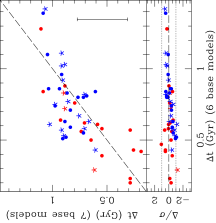
Appendix C Model tests

In order to assess the robustness of the parameter extraction, we compared the analysis presented in the paper – that combines six base models as presented in Sec. 3 – with a new run where one additional base model is included. The starting procedure is identical to the original method, performing a trial search that gives a best fit metallicity, used as reference for base models 1 through 6. These base models assume a constant star formation rate in the following age intervals:

• New Base Model 1: $\log t/{\rm Gyr}\in[-2,-1]$

• New Base Model 2: $\log t/{\rm Gyr}\in[-1,-1+\delta]$

• New Base Model 3: $\log t/{\rm Gyr}\in[-1+\delta,-1+2\delta]$

• New Base Model 4: $\log t/{\rm Gyr}\in[-1+2\delta,-1+3\delta]$

• New Base Model 5: $\log t/{\rm Gyr}\in[-1+3\delta,-1+4\delta]$

• New Base Model 6: $\log t/{\rm Gyr}\in[-1+4\delta,lt_{\rm MAX}]$

• New Base Model 7: $\log t/{\rm Gyr}\in[-1+4\delta,lt_{\rm MAX}]$,

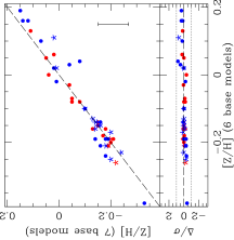
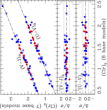
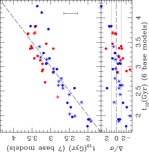
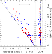
where $lt_{\rm MAX}$ is the log₁₀ of the age of the Universe (in Gyr) at the redshift of the galaxy, and $\delta\equiv(lt_{\rm MAX}+1)/5$. Analogously to the fiducial case, BM7 is defined over the same interval as BM6, but corresponding to a metallicity 0.3 dex lower than the reference. Fig. 15 shows a comparison of the best fit models between the 6 base model choice (horizontal axes) and the 7 base model runs (vertical axes). The bottom subpanel for each case shows the difference between these two models ($\Delta$), measured in units of the individual uncertainties ($\sigma$). The figure shows that, within the quoted error bars, the results are quite robust, especially regarding average age, oldest age and $\Delta t$. The colour excess parameters are also quite robust, as are the rest-frame colours adopted when segregating the sample with respect to star formation activity (Fig. 7). An accurate estimate of the colour excess mainly requires good flux calibration, as dust mainly affects the illumination source as a smooth wavelength-dependent function (see, e.g., Cardelli et al., 1989). In this regard, spectral resolution is not so important when constraining the colour excess. Due to its excellent flat fielding, the slitless grism data provided by the HST cameras allow us to produce spectra with very accurate flux calibration (see, e.g., Pirzkal et al., 2017).

Figure 15: Comparison of parameter fits by use of two different sets of models comprising 6 (our fiducial choice) and 7 base models (BM). For each case, as labelled, we show the parameter from the 7 BM (vertical) vs the 6 BM analysis (horizontal). The bottom subpanels show the difference ($\Delta$) of a given parameter between the 6 BM and the 7 BM fits, measured as a fraction of the quoted uncertainty ($\sigma$). A typical error bar is shown in each case (it is roughly the same in both, 6 and 7 base model runs). The sample is split with respect to visual morphology, with early-types shown as filled dots and late-types as star symbols. The sample is colour coded, with red (blue) galaxies representing quiescent (star-forming) galaxies, as shown in Fig. 9. The panel with the rest-frame colours – labeled (Clr)₀ – include both $(U-V)_{0}$ and $(V-J)_{0}$, where the latter – for the 7 BM runs – is shifted up by 1 mag to avoid crowding.

References

- Alexander et al. (2003) Alexander D. M., et al., 2003, AJ, 126, 539
- Belli, Newman, & Ellis (2015) Belli S., Newman A. B., Ellis R. S., 2015, ApJ, 799, 206
- Bezanson et al. (2013) Bezanson R., van Dokkum P., van de Sande J., Franx M., Kriek M., 2013, ApJ, 764, L8
- Boggs & Rogers (1990) Boggs, P. T., Rogers, J. E., 1990, Contemporary Mathematics, 112, 186
- Bruzual & Charlot (2003) Bruzual, A., Charlot, S., 2003, MNRAS, 344, 1000
- Cardelli et al. (1989) Cardelli J. A., Clayton G. C., Mathis J. S., 1989, ApJ, 345, 245
- Chabrier (2003) Chabrier, G., 2003, PASP, 115, 763
- Chabrier, Hennebelle, & Charlot (2014) Chabrier G., Hennebelle P., Charlot S., 2014, ApJ, 796, 75
- Charlot & Fall (2000) Charlot S., Fall S. M., 2000, ApJ, 539, 718
- Chauke et al. (2018) Chauke P., et al., 2018, ApJ, 861, 13
- Choi et al. (2014) Choi J., Conroy C., Moustakas J., Graves G. J., Holden B. P., Brodwin M., Brown M. J. I., van Dokkum P. G., 2014, ApJ, 792, 95
- Cimatti et al. (2004) Cimatti, A., et al., 2004, Nature, 430, 184
- Cimatti et al. (2008) Cimatti, A., et al., 2008, A&A, 482, 21
- Conroy (2013) Conroy C., 2013, ARA&A, 51, 393
- Conselice et al. (2008) Conselice C. J., Bundy K., U V., Eisenhardt P., Lotz J., Newman J., 2008, MNRAS, 383, 1366
- Daddi et al. (2005) Daddi E., et al., 2005, ApJ, 626, 680
- Díaz-García et al. (2018) Díaz-García L. A., et al., 2018, arXiv:1802.06813
- Dressler (1980) Dressler A., 1980, ApJ, 236, 351
- Estrada-Carpenter et al. (2018) Estrada-Carpenter, V, et al., 2018, arXiv, arXiv:1810.02824
- Ferreras & Silk (2000) Ferreras, I., Silk, J., 2000, MNRAS, 316, 786
- Ferreras, Saha & Burles (2008) Ferreras, I., Saha, P., Burles, S., 2008, MNRAS, 383, 857
- Ferreras et al. (2009) Ferreras I., et al., 2009, ApJ, 706, 158
- Ferreras et al. (2009) Ferreras I., Lisker T., Pasquali A., Kaviraj S., 2009, MNRAS, 395, 554
- Ferreras et al. (2012) Ferreras, I., et al., 2012, AJ, 144, 47
- Fitzpatrick (1999) Fitzpatrick, E. L., 1999, PASP, 111, 63
- Foreman-Mackey et al. (2013) Foreman-Mackey D., Hogg D. W., Lang D., Goodman J., 2013, PASP, 125, 306
- Fumagalli et al. (2016) Fumagalli, M., et al., 2016, ApJ, 822, 1
- Gallazzi et al. (2005) Gallazzi A., Charlot S., Brinchmann J., White S. D. M., Tremonti C. A., 2005, MNRAS, 362, 41
- Gallazzi et al. (2014) Gallazzi A., Bell E. F., Zibetti S., Brinchmann J., Kelson D. D., 2014, ApJ, 788, 72
- Grogin et al. (2011) Grogin, N. A., et al., 2011, ApJS, 197, 35
- Guo et al. (2011) Guo Y., et al., 2011, ApJ, 735, 18
- Huertas-Company et al. (2015) Huertas-Company, M., et al., 2015, ApJS, 221, 8
- Kartaltepe et al. (2015) Kartaltepe, J. S., et al., 2015, ApJS, 221, 11
- Kaviraj et al. (2005) Kaviraj S., Devriendt J. E. G., Ferreras I., Yi S. K., 2005, MNRAS, 360, 60
- Koekemoer et al. (2011) Koekemoer, A. M., et al., 2011, ApJS, 197, 36
- Kriek et al. (2016) Kriek M., et al., 2016, Nature, 540, 248
- Kroupa (2001) Kroupa P., 2001, MNRAS, 322, 231
- La Barbera et al. (2016) La Barbera F., Vazdekis A., Ferreras I., Pasquali A., Cappellari M., Martín-Navarro I., Schönebeck F., Falcón-Barroso J., 2016, MNRAS, 457, 1468
- La Barbera et al. (2017) La Barbera F., Vazdekis A., Ferreras I., Pasquali A., Allende Prieto C., Röck B., Aguado D. S., Peletier R. F., 2017, MNRAS, 464, 3597
- Labbé et al. (2005) Labbé I., et al., 2005, ApJ, 624, L81
- Luo et al. (2008) Luo B., et al., 2008, ApJS, 179, 19
- Madau & Dickinson (2014) Madau P., Dickinson M., 2014, ARA&A, 52, 415
- Martín-Navarro et al. (2015) Martín-Navarro I., La Barbera F., Vazdekis A., Falcón-Barroso J., Ferreras I., 2015, MNRAS, 447, 1033
- Oke & Gunn (1983) Oke J. B., Gunn J. E., 1983, ApJ, 266, 713
- Onodera et al. (2015) Onodera M., et al., 2015, ApJ, 808, 161
- Oser et al. (2010) Oser L., Ostriker J. P., Naab T., Johansson P. H., Burkert A., 2010, ApJ, 725, 2312
- Pasquali et al. (2006) Pasquali A., et al., 2006, ApJ, 636, 115
- Peng et al. (2002) Peng C. Y., Ho L. C., Impey C. D., Rix H.-W., 2002, AJ, 124, 266
- Pharo et al. (2018) Pharo J., et al., 2018, ApJ, 856, 116
- Pirzkal et al. (2017) Pirzkal, N., et al. 2017, ApJ, 846, 84
- Renzini (2006) Renzini A., 2006, ARA&A, 44, 141
- Salpeter (1955) Salpeter, E. E., 1955, ApJ, 121, 161
- Santini et al. (2015) Santini, P., et al., 2015, ApJ, 801, 97
- Scott et al. (2017) Scott N., et al., 2017, MNRAS, 472, 2833
- Shen et al. (2003) Shen S., Mo H. J., White S. D. M., Blanton M. R., Kauffmann G., Voges W., Brinkmann J., Csabai I., 2003, MNRAS, 343, 978
- Simha et al. (2014) Simha V., Weinberg D. H., Conroy C., Dave R., Fardal M., Katz N., Oppenheimer B. D., 2014, arXiv, arXiv:1404.0402
- Skelton et al. (2014) Skelton, R. E., et al. 2014, ApJ, 214, 24
- Stanford et al. (2004) Stanford S. A., Dickinson M., Postman M., Ferguson H. C., Lucas R. A., Conselice C. J., Budavári T., Somerville R., 2004, AJ, 127, 131
- Trujillo et al. (2006) Trujillo I., et al., 2006, ApJ, 650, 18
- Trujillo, Ferreras, & de La Rosa (2011) Trujillo I., Ferreras I., de La Rosa I. G., 2011, MNRAS, 415, 3903
- van de Sande et al. (2013) van de Sande J., et al., 2013, ApJ, 771, 85
- van der Wel et al. (2012) van der Wel A., et al., 2012, ApJS, 203, 24
- van Dokkum et al. (2008) van Dokkum P. G., et al., 2008, ApJ, 677, L5
- van Dokkum & Brammer (2010) van Dokkum P. G., Brammer G., 2010, ApJ, 718, L73
- van Dokkum et al. (2017) van Dokkum P., Conroy C., Villaume A., Brodie J., Romanowsky A. J., 2017, ApJ, 841, 68
- Vazdekis et al. (2012) Vazdekis, A., Ricciardelli, E., Cenarro, A J., Rivero-González, J. G., Díaz-García, L. A. D., Falcón-Barroso, J., 2012, MNRAS, 424, 157
- Williams et al. (2009) Williams R. J., Quadri R. F., Franx M., van Dokkum P., Labbé I., 2009, ApJ, 691, 1879
- Windhorst et al. (2011) Windhorst R. A., et al., 2011, ApJS, 193, 27