Statistical Trends in the Obliquity Distribution of Exoplanet Systems

Abstract

Important clues on the formation and evolution of planetary systems can be inferred from the stellar obliquity $\psi$. We study the distribution of obliquities using the California-Kepler Survey and the TEPCat Catalog of Rossiter-MacLaughlin (RM) measurements, from which we extract, respectively, 275 and 118 targets. We infer a “best fit” obliquity distribution in $\psi$ with a single parameter $\kappa$. Large values of $\kappa$ imply that $\psi$ is distributed narrowly around zero, while small values imply approximate isotropy. Our findings are: (1) The distribution of $\psi$ in Kepler systems is narrower than found by previous studies and consistent with $\kappa\sim 15$ (mean $\langle\psi\rangle\sim 19^{\circ}$ and spread $\psi\sim 10^{\circ}$). (2) The value of $\kappa$ in Kepler systems does not depend, at a statistically significant level, on planet multiplicity, stellar multiplicity or stellar age; on the other hand, metal rich hosts, small planet hosts and long-period planet hosts tend to be more oblique than the general sample (at a $\sim$2.5-$\sigma$ significance level). (3) Hot Jupiter (HJ) systems with RM measurements are consistent with $\kappa\sim 2$, more broadly distributed than the general Kepler population. (4) A separation of the RM sample into cooler ($T_{\rm eff}\lesssim$6250 K) and hotter ($T_{\rm eff}\gtrsim$6250 K) HJ hosts results in two distinct distributions, $\kappa_{\rm cooler}\sim 4$ and $\kappa_{\rm hotter}\sim 1$ (4-$\sigma$ significance), both more oblique than the Kepler sample. We hypothesize that the total mass in planets may be behind the increasing obliquity with metallicity and planet radius, and that the period dependence could be due to primordial disk alignment rather than tidal realignment of stellar spin.

1. Introduction

The alignment of planetary orbits with the spin axis of their host star is a fundamental feature of exoplanetary architectures; one that points directly to the physical mechanisms behind planetary formation. In the Solar System, for example, the Sun’s stellar spin is tilted with respect to the ecliptic by only $\sim 7^{\circ}$ (Carrington, 1863; Beck & Giles, 2005). Exoplanetary systems, on the other hand, may exhibit severe spin-orbit misalignments, including nearly polar orientations (e.g., Kepler-63b, Sanchis-Ojeda et al., 2013). A complete, predictive theory of planet formation must explain the origin of both large and small stellar obliquities, being able to discern whether these are inherited from the protoplanetary disk or if they are a consequence of later dynamical interactions.

The true, three-dimensional obliquity $\psi$ of a planet-hosting star is not a direct observable. This angle can be expressed as (e.g. Winn et al., 2007)

$$\cos\psi=\cos I_{*}\cos i_{\rm p}+\sin I_{*}\sin i_{\rm p}\cos\lambda$$ (1)

where $i_{\rm p}$ is the planet’s orbital inclination, $I_{*}$ is the stellar line-of-sight (LOS) inclination and $\lambda$ is the projected obliquity onto the plane of the sky. Typically, $\lambda$ is measured via the Rossiter–McLaughlin (RM; Rossiter, 1924; McLaughlin, 1924) effect (e.g., see Queloz et al., 2000; Ohta et al., 2005; Giménez, 2006), or even estimated via stellar spot variability (Nutzman et al., 2011), and can be related to $\psi$ via statistical arguments (Fabrycky & Winn, 2009). The stellar LOS inclination $I_{*}$ is more difficult to measure directly; it can be estimated from asteroseimology (Gizon & Solanki, 2003; Campante et al., 2016) or inferred from a combination of projected velocity measurements $V\sin I_{*}$, stellar radii $R_{*}$ and rotational periods $P_{\rm rot}$ (e.g. Winn et al., 2007; Hirano et al., 2014; Morton & Winn, 2014). Provided that stellar radii and rotational periods are available for a large number of stars (as is the case of the Kepler catalog; e.g., McQuillan et al., 2014), the $V\sin I_{*}$ approach to stellar obliquity inference is the most cost-effective, since $V\sin I_{*}$ measurements are easier to come about than RM ones: not only do they require less spectral resolution and sensitivity, but also do not need to be taken during transit (e.g., Gaudi & Winn, 2007)

An ensemble of either $\lambda$ or $I_{*}$ measurements facilitates statistical tests that can constrain to which degree planetary orbits tend to be aligned/misaligned with the spins of their host stars (Fabrycky & Winn, 2009; Morton & Winn, 2014; Campante et al., 2016). Spin-orbit statistics can also provide valuable tools for identifying distinct planet populations or for distinguishing between planet formation models. Focusing on the origins of hot Jupiters, Morton & Johnson (2011) compared the obliquity outcomes of two said models, the Lidov-Kozai migration of model of hot Jupiters by Fabrycky & Tremaine (2007) and the planet scattering scenario of Nagasawa et al. (2008), inferring that the scattering model more likely given the observations of projected obliquity.

As the number of obliquity measurements increases further, astronomers are able to identify other emerging trends that relate the distribution of obliquity to different planetary and stellar properties. One such trend is that of hot Jupiters tending to have smaller values of $\lambda$ when their host stars have effective temperatures below $T_{\rm eff}\sim 6000$-$6300$K (Winn et al., 2010; Albrecht et al., 2012, 2013, see also Winn & Fabrycky, 2015). This temperature dependence is the most robust obliquity relation in the literature, and it has been reflected not only in $\lambda$, but also in the distribution of photometric modulation amplitudes (Mazeh et al., 2015), which should depend on the orientation of the stellar spin axis (see also Li & Winn, 2016). Another possible trend relates hot Jupiter obliquity to stellar age (Triaud, 2011), and there is also evidence to suggest that hot Jupiters in general are more oblique than the general planet population (Albrecht et al., 2013, and more recently Winn et al., 2017). One intriguing finding, perhaps pointing to the dynamical evolution of planetary systems, is that stars with multiple planets may be very closely aligned (Sanchis-Ojeda et al., 2012; Albrecht et al., 2013) although it is unclear if the converse is true of single-transiting systems: Morton & Winn, 2014 noted a modest trend suggestive of higher obliquity in systems with one transiting planet, but very recently, Winn et al. (2017) reported that the trend has disappeared.

In the present work, we address the statistical trends mentioned above, and explore additional ones, making use of two publicly available catalogs: the California-Kepler Survey (Petigura et al., 2017; Johnson et al., 2017) and the TEPCat database (Southworth, 2011).

2. Obliquity Distribution from Bayesian Inference

2.1. The Geometry of Stellar Obliquity

The stellar obliquity $\psi$ is the angle between the stellar spin vector $\mathbf{S}_{*}$ and the planetary orbit’s angular momentum vector $\mathbf{L}_{\rm p}$. The three-dimensional orientation of $\mathbf{S}_{*}$ in space is determined by a polar angle $\theta$ and an azimuthal angle $\phi$. Observationally, however, instead of $\theta$ and $\phi$, it is more convenient to work in terms of $I_{*}$, the angle between $\mathbf{S}_{*}$ the LOS, and $\beta_{*}$, the projected angle of $\mathbf{S}_{*}$ onto the plane of the sky. These angles are related by:

$$\cos I_{*}=\sin\theta\cos\phi~{}~{},$$ (2a)

$$\sin I_{*}\sin\beta_{*}=\sin\theta\sin\phi~{}~{},$$ (2b)

$$\sin I_{*}\cos\beta_{*}=\cos\theta~{}~{}.$$ (2c)

Now, for transiting planets, one can assume that $i_{\rm p}\approx 90^{\circ}$ (cf. Eq. 1), i.e., $\mathbf{L}_{\rm p}$ is perpendicular to the LOS; this assumption allows us to set $\theta=\psi$ and $\beta_{*}=\lambda$, where $\lambda$ is the projected spin-orbit misalignment angle.

In the following, we describe how a collection of $\lambda$ or $\cos I_{*}$ measurements can be used to constrain the statistical properties of the true obliquity $\psi$.

2.2. The Fisher Distribution for $\psi$ and the Concentration Parameter

We are interested in finding the distribution of obliquities for a sample of known exo-planetary systems. For this, it is convenient to have a model function, such as the Fisher distribution (Fisher, 1953; Fisher et al., 1993), which was proposed for exoplanet obliquities by Fabrycky & Winn (2009) (see also Tremaine & Dong, 2012) and has the form

$$f_{\psi}(\psi|\kappa)=\frac{\kappa}{2\sinh\kappa}\exp(\kappa\cos\psi)\sin\psi$$ (3)

where $\kappa$ is often referred to as the “concentration parameter”. The Fisher distribution of Eq. (3) does not have closed-form expressions for its moments. The mean $\langle\psi\rangle$ and standard deviation $\sigma_{\psi}\equiv\sqrt{\langle\psi^{2}\rangle-\langle\psi\rangle^{2}}$ are shown in Fig. 1 as a function of $\kappa$. For large $\kappa$, $f_{\psi}(\psi|\kappa)$ reduces to the Rayleigh distribution with scale parameter $\sigma\equiv\kappa^{-1/2}$, for which $\langle\psi\rangle=\sqrt{{\pi}/{2}}\sigma$ and $\sigma_{\psi}=\sqrt{2-\tfrac{\pi}{2}}\sigma$. Thus, the quantity $\kappa^{-1/2}$ provides a scale for the mean and spread of the obliquity angle.

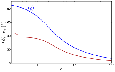
Figure 1.— Moments of the Fisher distribution (Eq. 3) in degrees. The mean obliquity $\langle\psi\rangle$ for a given value of $\kappa$ is depicted in blue; the spread (standard deviation) of obliquity $\sigma_{\psi}$ given $\kappa$ is depicted in red. When $\kappa=0$ (isotropy), $\langle\psi\rangle=90^{\circ}$ and $\sigma_{\psi}=({\pi^{2}/4-2})^{1/2}\approx 39.17^{\circ}$. When $\kappa\gtrsim 30$, $f_{\psi}$ approximates a Rayleigh distribution with $\langle\psi\rangle\approx\sqrt{{\pi}/{2}}\kappa^{-1/2}$ and $\sigma_{\psi}=(4/\pi-1)^{1/2}\sqrt{{\pi}/{2}}\kappa^{-1/2}$.

Given the actual observable angles, it is convenient to work with the probability distributions of $\cos I_{*}$ or $\lambda$. Morton & Winn (2014) (hereafter MW14) have shown that, by means of Eq. (2a) and standard probability rules, one can derive $f_{\cos I_{*}}(z=\cos I_{*}|\kappa)$ in closed form:

$$f_{\cos I_{*}}(z|\kappa)=\frac{2\kappa}{\pi\sinh\kappa}\int\limits_{z}^{1}\frac{\cosh(\kappa\sqrt{1-y^{2}})}{\sqrt{1-y^{2}}}\frac{1}{\sqrt{1-(z/y)^{2}}}dy$$ (4)

which is normalized in such a way that $\cos I_{*}\in[0,1]$. In this work (see Appendix A), we also show that a similar derivation can be carried out to compute the PDF of the projected obliquity $\lambda$ given $\kappa$:

$$\begin{split}f_{\lambda}(\lambda|\kappa)&=\frac{\kappa}{2\pi\sinh\kappa}\frac{1}{\cos^{2}\lambda}\int\limits_{0}^{\cos\lambda}\frac{\exp(\kappa{y})}{\sqrt{1-{y}^{2}}}\frac{{y}}{\sqrt{1-\left(\tfrac{{y}^{2}}{1-{y}^{2}}\right)\tan^{2}\lambda}}d{y}\end{split}$$ (5)

normalized to be valid in the range $\lambda\in[-\pi,\pi]$. To the extent of our knowledge, this expression for $f_{\lambda}(\lambda|\kappa)$ has not been presented previously in the literature.

2.3. Hierarchical Bayesian Inference

For a given dataset $D$ containing $N$ stars with $N$ measurement posteriors of some quantity that depends on $\psi$ given $\kappa$, we write the total likelihood as

$$\mathcal{L}_{\kappa}=\prod\limits_{n=1}^{N}\mathcal{L}_{\kappa,n}~{}~{}.$$ (6)

The contribution from each measurement $\mathcal{L}_{\kappa,n}$ to the total likelihood $\mathcal{L}_{\kappa}$ depends on the stellar quantity being measured. If we have posteriors for $z=\cos I_{*}$, then we have (e.g. Hogg et al., 2010)

$$\mathcal{L}_{\kappa,n}(D|\kappa)\propto\int_{0}^{1}dz\,p(z|D_{n})\cfrac{f_{\cos I_{*}}(z|\kappa)}{\pi_{\cos I_{*},0}(z)}$$ (7)

where $\pi_{\cos I_{*},0}(z)=1$ for all $z$ is an uninformative prior. Similarly, for another dataset $\widetilde{D}$ from which $N$ posteriors on $\lambda$ can be obtained, we have

$$\mathcal{L}_{\kappa,n}(\widetilde{D}|\kappa)\propto\int_{-\pi}^{\pi}d\lambda\,p(\lambda|\widetilde{D}_{n})\cfrac{f_{\lambda}(\lambda|\kappa)}{\pi_{\lambda,0}(z)}$$ (8)

where the prior $\pi_{\lambda,0}(z)=1/(2\pi)$ is also uninformative and thus only amounts to a normalization constant. These two likelihoods (Eqs. 7 and 8) can be computed by direct numerical integration or by the method of $K$-samples (see Eq. B4).

The prior PDF of the meta-parameter $\kappa$ that must multiply the total likelihood in Eq (6) is usually assumed to take the form (Fabrycky & Winn, 2009):

$$\pi_{\kappa}(\kappa)\propto{(1+\kappa^{2})^{-3/4}}~{}~{}.$$ (9)

This prior is chosen to be well behaved when $\kappa=0$ and to become uniform in the Rayleigh scale parameter $\sigma=\kappa^{-1/2}$ as $\kappa\rightarrow\infty$. This prior may underestimate $\kappa$ if it is large ($\gg 10$), and a flat prior might pick up the signal of a large concentration parameter if the dataset is small (Campante et al., 2016). An alternative is to device a prior that, for large $\kappa$, the prior becomes logarithmic uninformative in $\sigma$ (i.e., a Jeffreys prior on a scale parameter) rather than uniform. This can be accomplished with a prior in $\kappa$ of the form

$$\pi^{\prime}_{\kappa}\propto{(1+\kappa^{2})^{-1/2}}~{}~{},$$ (9b)

which satisfies $\pi_{\sigma}\propto 1/\sigma$ for $\kappa\gg 1$. For the sake of consistency with previous studies, we will employ the prior function of Eq. (9) unless stated otherwise. As it turns out, the dataset is large enough that the inference on $\kappa$ is weakly sensitive to the choice of either prior. Further details of the Bayesian computation are provided in Appendix B.

We note that, in principle, inference using $\cos I_{*}$ and $\lambda$ simultaneously could be done by writing a two-dimensional integral for $\mathcal{L}_{\kappa,n}$ in place of Eqs. (7)-(8) and using a joint probability $p(z,\lambda|\kappa)=f_{\cos I_{*}}(z|\kappa)\times f_{\lambda}(\lambda|\kappa)$, where measurement posteriors for both $\cos I_{*}$ and $\lambda$ can be obtained for every object. Unfortunately, the number of Kepler systems for which both $\cos I_{*}$ and $\lambda$ has been derived/measured is small (we identify 5 such objects in Section 3.2). Thus, for the remainder of the paper, we will compute $p(\kappa|D)$ for the different datasets independently, acknowledging that each data set might sample different population planetary system and thus differences in the inferred values of $\kappa$ are to be expected.

3. Obliquity Distribution from Observations

3.1. The California Kepler Survey

Recently, Winn et al. (2017) used the California-Kepler Survey (CKS; Petigura et al., 2017; Johnson et al., 2017) to study the statistical properties of line-of-sight inclination $I_{*}$ and projected rotational velocity $V\sin I_{*}$ of numerous Kepler planet hosts. The extensive analysis of Winn et al. (2017) did not include inference on the concentration parameter $\kappa$ (Eq. 3), thus, the analysis presented below is highly complementary to their work.

We are interested in objects for which $V\sin I_{*}$, the stellar radius $R_{*}$ and the rotational period $R_{*}$ are known. The CKS catalog contains 1305 KOIs with $V\sin I_{*}$ and $R_{*}$ measurements, of which 773 have a “confirmed planet” disposition (Petigura et al., 2017). To assign rotational periods, we collect $P_{\rm rot}$ measurements from two main catalogs: Mazeh et al. (2015), which obtained via auto-correlation function analysis, and Angus et al. (2018), who introduced a novel Bayesian parameter estimation of $P_{\rm rot}$ as part of a parametric model consisting of a quasi-periodic Gaussian random process (QPGP). We are able to find additional periods in the literature, recovering measurements from Bonomo & Lanza (2012), McQuillan et al. (2013), McQuillan et al. (2014), Hirano et al. (2014), García et al. (2014), Paz-Chinchón et al. (2015) and Buzasi et al. (2016), all of which were obtained using somewhat different, but still deeply related methods. Most of these period identification techniques are based on Fourier analysis of time series (see discussion in Aigrain et al., 2015), with one departure being the Morlet wavelet method of García et al. (2014), which is still inherently a spectral analysis method. We refer to all these strategies collectively as “spectral analysis” (SA) methods and group the corresponding periods along with the Mazeh et al. (2015) catalog, leaving the Angus et al. (2018) catalog as the one truly distinct approach to period identification. Of the 773 entries in the CKS sample, we are able to assign SA periods for 734, and QPGP periods for 645; 614 targets have both SA and QPGP periods. Following Winn et al. (2017), we proceed with our analysis only using targets with “reliable” periods, meaning those for which SA and QPGP estimates coincide. Our period selection method is analogous although slightly more permissive that the one used by Winn et al. (2017). First, we only consider period measurements with a signal-to-noise ratio of 3 and larger. Second, we consider that the two period estimates match if they are within 30$\%$ of the identity, provided that the uncertainties overlap (we use 3-$\sigma$ error bars). Period filtering removes 492 targets, and we are left with 291. Possibly blended sources within the Kepler photometric aperture ($\sim 4^{\prime\prime}$ Mullally et al., 2015; Furlan et al., 2017) means that we cannot attribute the rotational period to the planet host; therefore, we remove 34 additional targets for which a nearby companion was detected by Furlan et al. (2017) within 3 mag of that of the target KIC star (Winn et al., 2017). We are left with a database of 257 targets.

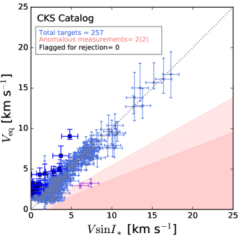
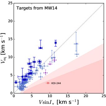
Figure 2.— Top panel: Inferred equatorial rotational velocities $V_{\rm eq}$ and their $68\%$ confidence intervals (see text) versus $V\sin I_{*}$ measurements and their uncertainties for 257 KOIs in the CKS (Petigura et al., 2017). Data points cluster around the identity, as it is to be expected from low obliquity systems. Seventeen systems with statistically significant misalignment ($I_{*}(95\%)\leq 86^{\circ}$) are depicted by large, dark blue squares, the rest of the objects are depicted by small, light blue squares. Two data points appear to be anomalous (in purple), as they lie below the identity at a distance of more than 3-$\sigma$ (but less than 5-$\sigma$) according to their own uncertainties. The two shaded areas are defined by the curves $V_{\rm eq}=V\sin I_{*}/1.8$ (upper) and $V_{\rm eq}=V\sin I_{*}/2.6$ (lower) and serve as target rejection boundaries. We define a criterion for target removal in which all data points for which the $95\%$ upper limit in $V_{\rm eq}$ lies below the first curve are rejected. In the 257-target dataset we generated from the CKS catalog, no object is flat-out rejected. Bottom panel: Same as above, but for the 70-target dataset of MW14. In that work, 12 targets are identified as misaligned with respect to the planetary orbits (i.e., confidently different from edge-on), 3 are anomalous, and 1 (KOI-244) is regarded as unphysical and thus rejected.

3.1.1 Inclination Posterior for Each Target

For each of the 257 CKS targets, we derive a posterior PDF of the line-of-sight inclination. In principle, the value of $I_{*}$ can be obtained from the straightforward operation

$$\sin I_{*}=\frac{(V\sin I_{*})}{V_{\rm eq}}=\frac{(V\sin I_{*})}{2\pi R_{*}/P_{\rm rot}}$$ (10)

(e.g. Borucki & Summers, 1984; Doyle et al., 1984; Soderblom, 1985; Winn et al., 2007; Albrecht et al., 2011). However, this approach has been long recognized as nontrivial because the often large uncertainties in the different quantities involved.

As described in detail by MW14, if one has PDFs for the projected rotational velocity $V\sin I_{*}$ and the equatorial rotational velocity $V_{\rm eq}$ – $p_{V_{s}}$ and $p_{V_{\rm eq}}$ respectively– the posterior PDF of $\sin I_{*}$ given a prior $\pi_{\sin I_{*}}(z)=z/\sqrt{1-z^{2}}$ (i.e., uniform in $\cos I_{*}$) is given by,

$$\begin{split}p(\sin I_{*}|D)\propto&~{}~{}\mathcal{L}(\sin I_{*})\pi_{\sin I_{*}}(\sin I_{*})\\ =&~{}~{}\frac{\sin I_{*}}{\sqrt{1-\sin^{2}I_{*}}}\int_{0}^{\infty}v^{\prime}p_{V_{s}}(v^{\prime}\sin I_{*})p_{V_{\rm eq}}(v^{\prime})dv^{\prime}~{}~{}.\end{split}$$ (11)

It is convenient to work in terms of $\cos I_{*}$. Since $p(\cos I_{*}|D)=p(\sin I_{*}|D)|\tfrac{d\sin I_{*}}{d\cos I_{*}}|$, the desired posterior is

$$\begin{split}p(\cos I_{*}|D)=&p(\sin I_{*}|D)\frac{\cos I_{*}}{\sqrt{1-\cos^{2}I_{*}}}\\ \propto&~{}~{}\int_{0}^{\infty}v^{\prime}p_{V_{s}}(v^{\prime}\sqrt{1-\cos^{2}I_{*}})p_{V_{\rm eq}}(v^{\prime})dv^{\prime}~{}~{}.\end{split}$$ (12)

MW14 assume $p_{V_{s}}(\cdot)$ is a Gaussian, but for $p_{V_{\rm eq}}(\cdot)$, they derive an empirical PDF from the Monte Carlo sampling of $P_{\rm rot}$ and $R_{*}$ -both assumed to be (double-sided) Gaussians– after incorporating the effects of differential rotation and the stochasticity of stellar spots. From the PDF $p_{V_{\rm eq}}$, we derive a most likely value $V_{\rm eq}$ and a confidence interval and plot it against the measured value of $V\sin I_{*}$; this is shown in Fig. 2 (top panel). All targets above the $V_{\rm eq}=V\sin I_{*}$ line (i.e., $\sin I_{*}<1$) are not edge-on (and potentially misaligned with respect to the planetary orbits). Targets for which $\sin I_{*}<1$ with some statistical certainty are highlighted. Targets below the $V_{\rm eq}=V\sin I_{*}$ line (i.e., $\sin I_{*}>1$) are unphysical if the uncertainties cannot account for such a measurement (see figure caption for further details). Fig. 2 (bottom panel) depicts the same comparison of velocities, but for the MW14 database. In our final 257-target database, two targets – KOIs 94 and 1848 (Kepler-89 and Kepler-978 respectively) – appear to be marginally unphysical, i.e., they are below the identity line at a distance greater than 3-$\sigma$ but smaller than 5-$\sigma$. We deem these two targets “anomalous”, but we do not remove them. Note that in the MW14 database, four targets are anomalous, but only one (KOI 244) is removed from their analysis. If not filtered out, anomalous targets will still have well behaved $\cos I_{*}$ PDFs (Eq. 12) that strongly peak at $\cos I_{*}=0$ (see Fig. 3 below), and favor lower values of $\kappa$ when entering Eq. (7).

The 257 PDFs of $\cos I_{*}$ are shown in Fig. 3. Of all these targets, only 17 (highlighted curves) have $I_{*}\neq 90^{\circ}$ to a $95\%$ confidence level (e.g., see MW14). This fraction ($6.6\%$) is lower than in the 70-target sample of MW14, which concluded that the number of misaligned (not edge-on) stars was 12 (or $17\%$). We thus expect the overall population to have lower mean obliquities, or a higher value of $\kappa$ in the distribution of Eq. (3), than originally reported by MW14.

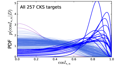
Figure 3.— Posterior PDFs of $\cos I_{*}$ (Eq.12) for the 257 targets in the dataset we compiled from the CKS catalog. The 17 targets that have LOS inclinations significantly different from edge-on are highlighted. The two targets that are partially anomalous (KOIs 94 and 1848; purple data points in Fig. 2) have PDFs that are strongly concentrated toward $\cos I_{*}=0$. Statistically significant…

3.1.2 Obliquity Distribution

With the 257 $\cos I_{*}$ posteriors depicted in Fig. 3, we can carry out the hierarchical Bayesian inference method summarized in Section 2. The likelihood of the data given $\kappa$ is computed from Eqs. (6) and (7), and the prior used is given by Eq. (9). The resulting posterior PDF of $\kappa$ is shown in Fig. 4, with a (weighted) maximum a posteriori of 14.5 and a shortest $68\%$-probability interval of $\kappa\in[8.5,28.0]$; thus, we write $\kappa_{\text{\tiny CKS}}=14.5^{+13.5}_{-6}$. This concentration parameter is significantly larger than the value reported by MW14, which we re-derived to be $\kappa_{\text{\tiny MW}}=6.2^{+1.8}_{-1.6}$. A value of $\kappa=15$ in Eq. (3) corresponds to a mean obliquity of $\langle\psi\rangle=19^{\circ}$ and a standard deviation of $\sigma_{\psi}=10^{\circ}$, while $\kappa=6$ results in $\langle\psi\rangle=30^{\circ}$ and $\sigma_{\psi}=16^{\circ}$. This “flattening” of the obliquity distribution might be a natural consequence of a larger number of systems with smaller planets being added to the list, revealing that the vast majority of systems have low obliquities. If we had removed KOIs 95 and 1848 (which are marginally unphysical and favor low obliquities; purple data points in Figs.2 and 3) we would have obtained $\kappa_{\text{\tiny CKS}}=13.8^{+12.2}_{-3.8}$, and thus their influence on $\kappa$ is negligible. We have also checked the influence of the prior function $\pi_{\kappa}$ of Eq. (9) versus the alternative prior $\pi_{\kappa}^{\prime}$ of Eq. (9b). If $\pi_{\kappa}^{\prime}$ is used, we find that the posterior $p(\kappa|D)$ produces $\kappa_{\text{\tiny CKS}}=15.4^{+23.8}_{-6.6}$, as expected from $\pi^{\prime}_{\kappa}$ being a more slowly declining function of $\kappa$, but a minor change considering the uncertainties. Up to this point, we can conclude that the CKS test is more spin-orbit aligned than the dataset used by MW14 and that the sample is consistent with obliquities in the range $\psi=(19\pm 10)^{\circ}$, provided that the Fisher distribution is an adequate model (see below).

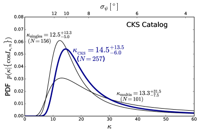
Figure 4.— Posterior PDF of the $\kappa$ parameter (Eq. 6 multiplied by Eq. 9 using Eq. 7) in dark blue. The distribution is summarized by the representative value of 14.4 and a $68\%$-probability interval $[8.8,28]$, i.e., $\kappa_{\text{\tiny CKS}}=14.5^{+13.5}_{-6}$. In addition, we present the $\kappa$ posterior from two subsets: systems with one transiting planet and systems with multiple transiting planets. The two subsets produce virtually indistinguishable concentration parameter PDFs (thin black curves), suggesting that the underlying obliquity does not depend on planet multiplicity.

A tentative trend discovered by MW14, which now seems to have disappeared (Winn et al., 2017), is that of $\kappa$ having a dependence on planet multiplicity. In Fig. 4, we show the separation of the CKS dataset into a subset containing “singles” (systems with one transiting planet) and one containing “multis” (systems with multiple transiting planets). Indeed, the multiplicity trend no longer appears to be real, as we find $\kappa^{\text{\tiny CKS}}_{\rm singles}=12.2^{+12.3}_{-5}$ and $\kappa^{\text{\tiny CKS}}_{\rm multis}=13.3^{+31.5}_{-7.5}$, i.e., the two posterior PDFs are indistinguishable.

Model Selection

Despite its useful functional form, the Fisher distribution (Eq. 3) is not fully justified on physical grounds and, in principle, other obliquity distributions could fit the data better. Fabrycky & Winn (2009) considered alternative models, such as a mixture of Fisher distributions or a mixture of an isotropic distribution and a spin-orbit aligned one. A mixture model of two Fisher distributions (two concentration parameters $\kappa_{1}$ and $\kappa_{2}$ with relative weights $f$ and $1{-}f$) has a joint posterior PDF given by

$$\begin{split}p(\kappa_{1},\kappa_{2},f|D)&\propto p(D|\kappa_{1},\kappa_{2},f)\times\pi(\kappa_{1},\kappa_{2},f)\\ &\propto\left[\prod\limits_{n=1}^{N}{\mathcal{L}}_{\boldsymbol{\alpha},n}(D_{n}|\kappa_{1},\kappa_{2},f)\right]\pi(\kappa_{1})\pi(\kappa_{2})\pi(f)\end{split}$$ (13)

where the contribution of the $n$-th measurement to the total likelihood is

$${\mathcal{L}}_{\boldsymbol{\alpha},n}(D_{n}|\kappa_{1},\kappa_{2},f)=f{\mathcal{L}}_{\kappa,n}(D_{n}|\kappa_{1})+(1-f){\mathcal{L}}_{\kappa,n}(D_{n}|\kappa_{2})$$ (14)

where ${\mathcal{L}}_{\kappa,n}(D_{n}|\kappa_{1})$ is given by Eq. (7). In Eq. (13) we have also assumed that the three-parameter prior $p(\boldsymbol{\alpha})=p(\kappa_{1},\kappa_{2},f)$ is separable. Figure 5 shows the joint posterior of $\kappa_{1}$ and $\kappa_{2}$ and the marginalized posterior of $f$. The marginalized “best fit” values are $\kappa_{1}=0^{+11.4}_{-0}$, $\kappa_{2}=18.4^{+17.6}_{-7.2}$ and $f=0.02^{+0.21}_{-0.02}$. This roughly states that the data areconsistent with a small fraction of the population (a few percent, consistent with 17 of of 257 targets being oblique; see Fig. 3) being drawn from a high-obliquity distribution and a large fraction of the population being drawn from a low-obliquity distribution.

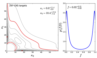
Figure 5.— Posterior PDF for the two-Fisher mixture model of three parameters $\kappa_{1}$, $\kappa_{2}$ and $f$ (Eq. 13). Left panel: joint posterior PDF of $\kappa_{1}$ and $\kappa_{2}$ after marginalizing over $f$. Right panel: the posterior of $f$ after marginalizing over $\kappa_{1}$ and $\kappa_{2}$. The $\kappa_{1}$-$\kappa_{2}$ mirroring symmetry is expected from the model, as is the symmetry of $f$ around 0.5. For simplicity, we report on the posterior results assuming $\kappa_{1}<\kappa_{2}$, which correspond to $f$ peaking close to zero.

To compare this new model (which we call $\mathcal{M}_{1}$) with the previous, simpler one ($\mathcal{M}_{0}$), we need to compute

$$p(D|\mathcal{M})=\int p(D|\kappa_{1},\kappa_{2},f)\pi(\kappa_{1},\kappa_{2},f)d\kappa_{1}d\kappa_{2}df$$ (15)

(sometimes called the “Bayesian evidence”) and then calculate the posterior odds ratio:

$$\begin{split}\frac{p(\mathcal{M}_{0}|{D})}{p(\mathcal{M}_{1}|{D})}&=\underbrace{\frac{p(D|\mathcal{M}_{0})}{p(D|\mathcal{M}_{1})}}\frac{p(\mathcal{M}_{0})}{p(\mathcal{M}_{1})}\\ &~{}~{}~{}~{}~{}~{}\equiv\mathcal{K}\end{split}$$ (16)

where $\mathcal{K}$ is called the “Bayes factor” or ”evidence ratio”. If we assume that $p(\mathcal{M}_{0})=p(\mathcal{M}_{1})=1/2$, then the model choice is given by $\mathcal{K}$. We find that $\mathcal{K}=2.25$, and thus, the data supports the null (simplest) model $\mathcal{M}_{0}$ in favor of the alternative model $\mathcal{M}_{1}$ (although not decisively, see Jeffreys, 1961, appendix B).

Alternatively, since one of the concentration parameters in $\mathcal{M}_{1}$ is consistent with zero, we can take $\kappa_{1}=0$ and create another mixture model ($\mathcal{M}_{2}$) consistent of an isotropic distribution and a Fisher distribution (e.g., see Campante et al., 2016). The likelihood function of the $n$-th target becomes

$${\mathcal{L}}_{\boldsymbol{\alpha},n}(D_{n}|\kappa,f)=f+(1-f){\mathcal{L}}_{\kappa,n}(D_{n}|\kappa)$$ (17)

The posterior distribution of this simpler model (of only two parameters) produces $\kappa=18.1^{+17.4}_{-6.9}$ and $f=0.02^{+0.04}_{-0.01}$. The evidence ratio, in this case, is $\mathcal{K}=p(D|\mathcal{M}_{0})/p(D|\mathcal{M}_{2})=12$. Thus, the null model $\mathcal{M}_{0}$ is substantially favored by the data.

In what follows, we explore the obliquity properties of different subsets – say $D_{A}$ and $D_{B}$ where $\cup\{D_{i}\}=D$ – within the CKS catalog. Our aim is to assess whether a given subset is “more oblique” or “less oblique” than its complement. Although we derive different values/posteriors of $\kappa_{A}$ and $\kappa_{B}$, our main goal is not to analyze the physical meaning of each concentration parameter, but to measure the statistical significance of the differences encountered.

3.1.3 Obliquity Trends: Stellar Properties

The larger size of the CKS set with respect to previously published catalogs allows us to explore changes in $\kappa$ as a function of different physical variables. In the following, we focus on the properties of the stellar host.

Effective Temperature

One intriguing stellar property that appears to affect the obliquity of planetary systems is the stellar effective temperature (Schlaufman, 2010; Winn et al., 2010; Albrecht et al., 2012, 2013; Mazeh et al., 2015; Winn et al., 2017). This transition appears to coincide with the so-called “Kraft break” (Struve, 1930; Schatzman, 1962; Kraft, 1967), identified as a sharp increase in the measured projected velocities in the field at around $T_{\rm eff}=$6200 K. This break is attributed to the transition that takes place when the width of the convective envelope of a Solar type star vanishes, giving rise to radiative envelopes at higher temperatures. We explore the temperature dependence in our compiled list of 257 Kepler targets. Placing a cut at 6200 K, we divide the dataset into “hotter” systems ($T_{\rm eff}\geq$6200 K) and “cooler systems” ($T_{\rm eff}<$6200 K), with 20 and 237 targets respectively. We find no statistical difference: we derive $\kappa^{\text{\tiny CKS}}_{\rm hotter}=15.2^{+46}_{-10.4}$ and $\kappa^{\text{\tiny CKS}}_{\rm cooler}=12.2^{+8.6}_{-4.2}$. However, this inference is largely due to the small number on KOIs with effective temperatures above 6200 K. This lack of detected planets around “hotter” stars is at least in part due to a selection effect, since those hot stars for which planetary transits are detected tend to be the least variables ones, in turn preventing the measurement of their rotational periods from photometric variability (Mazeh et al., 2015; Winn et al., 2017). We return to this subject in Section 3.2 below.

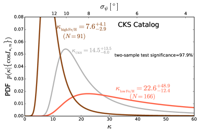
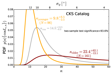
Figure 6.— Separation of the 257-target dataset into two subsets according to stellar metallicity (Petigura et al., 2018) and stellar age (ages from Johnson et al., 2017) in the CKS survey. Top panel: separation onto high-$Z$ systems ([Fe/H]$>=0.135$, $N=$ objects) and low-$Z$ systems ([Fe/H]$<0.135$, $N=$ objects). The concentration parameter of the younger subset is $9.8$ (i.e., $\langle\psi\rangle\approx 23^{\circ}$ and $\sigma_{\psi}\approx 12^{\circ}$), and that of the older subset is $22.6$ (i.e., $\langle\psi\rangle\approx 15^{\circ}$ and $\sigma_{\psi}\approx 8^{\circ}$); the statistical significance of this difference is 97.9$\%$. Bottom panel: splitting of the dataset into younger (yellow) and older (dark red) KOIs (ages from Johnson et al., 2017). The age cutoff chosen to separate the dataset is $\log A_{\rm cut}=9.63$ (or $A=4.27$ Gyr). The concentration parameter of the younger subset is $9.8$ (i.e., $\langle\psi\rangle\approx 23^{\circ}$ and $\sigma_{\psi}\approx 12^{\circ}$), and that of the older subset is $22.4$ (i.e., $\langle\psi\rangle\approx 15^{\circ}$ and $\sigma_{\psi}\approx 8^{\circ}$); the statistical significance of this difference is only 93.5$\%$ (a 1.85-$\sigma$ detection). The overlap between the low-metallicity sample ($N=166$) and the older sample ($N=161$) is significant but not overwhelming; 103 objects satisfy both [Fe/H]$<0.135$ and $\log A>9.63$.

Metallicity

The high precision provided by the CKS survey allows us to explore the impact of other fundamental stellar properties such as metallicity and age. In principle, these two variables are not entirely independent from each other, as we expect the older sample to have somewhat lower metallicity than the younger sample. However, the dynamical range in age is too narrow to reveal any correlation with metallicity; furthermore, both the lowest and highest metallicities in the sample, [Fe/H]$=-0.4\pm 0.04$ for KOI-623 and [Fe/H]$=0.396\pm 0.04$ for KOI-941, have “old” ages of $\log A=9.95_{-0.13}^{+0.08}$ and $\log A=10.03_{-0.27}^{+0.12}$ respectively. Fig. 6 (top panel) shows the concentration inference for a separation of the dataset into a low-metallicity sample ($N=166$) and a high-metallicity one ($N=91$). The cut in metallicity is [Fe/H]${}_{\rm cut}=0.135$, and is chosen as the one that maximizes the difference in the obliquity properties of the two subsamples, i.e., the value of cutoff is a free parameter, which is explored in a “sweeping” fashion. Inference results in a concentration parameter of $\kappa^{\text{\tiny CKS}}_{\text{\tiny low [Fe/H]}}=22.6^{+48.9}_{-12.4}$ for the lower metallicity subsample, and $\kappa^{\text{\tiny CKS}}_{\text{\tiny high [Fe/H]}}=7.6^{+4.1}_{-2.9}$ for the higher metallicity one. The two PDFs appear different, and thus a proper statistical assessment of their true distinctiveness is required. Following MW14, we use the squared Hellinger distance $\delta_{{\rm H}^{2}}$ as a difference metric between the two distributions. Then, we repeat the hierarchical inference 5000 times by Monte Carlo sampling the dataset in a way that two samples $D_{1}$ and $D_{2}$ of sizes $N_{1}=166$ and $N_{2}=91$ are generated at random for each try. For each of these tries, we compute $p(\kappa_{1}|D_{1})$ and $p(\kappa_{2}|D_{2})$, and measure the corresponding $\delta_{{\rm H}^{2}}$. We then count the fraction of realizations in which the synthetic $\delta_{{\rm H}^{2}}$ is equal or larger than in the real sample. This test quantifies the likelihood of obtaining the observed difference between $\kappa^{\text{\tiny CKS}}_{\text{\tiny low [Fe/H]}}$ and $\kappa^{\text{\tiny CKS}}_{\text{\tiny high [Fe/H]}}$ by mere chance. We find that in $\sim 2\%$ of the random tries, the two resulting PDFs are more different than in the top panel of Fig. 6 (by measure of $\delta_{{\rm H}^{2}}$), thus concluding that this difference is $98\%$ significant (i.e., a 2.3-$\sigma$ detection) and thus suggestive, but not conclusive. Difference in the planet-bearing frequency as a function of metallicity have been reported in the literature (e.g., Mulders et al., 2016; Petigura et al., 2018), and thus the (moderate) trend of $\kappa$ with [Fe/H] might be an indirect reflection of a dependence of $\kappa$ on planet type (see Section 3.1.4 below). For example, one might expect, qualitatively, that larger and more numerous rocky cores are formed in high metallicity protoplanetary disks (Petigura et al., 2018). The lower values of $\kappa$ at higher metallicities might be linked to the formation of more crowded/tightly packed systems, that will tend to be less stable (e.g. Pu & Wu, 2015), thus evolving toward excited mutual inclinations and obliquities.

Age

Stellar obliquity can be affected by stellar spin-down as well as by tidal coupling to close-in planets (e.g. Winn et al., 2010; Dawson, 2014; Albrecht et al., 2013; Li & Winn, 2016), both of which act over long periods of time. Thus, provided that accurate estimates and a wide enough ranges of stellar ages are available, one can in principle probe for changes in $\kappa$ as a function of this quantity (e.g., see Triaud, 2011). As a part of the CKS, Johnson et al. (2017) fitted evolutionary models to the observed spectroscopic parameters to obtain stellar masses and ages. We add theses ages to the 257 target samples and split the dataset into an “older” subset ($\log A\geq\log A_{\rm cut}=9.63$) with $N=161$ targets and a “younger” subset ($\log A<\log A_{\rm cut}$) with $N=96$ targets, where the cutoff value was deliberately chosen as the one that maximizes the statistical significance of the data splitting. We show the results of the concentration inference as a function of age in Fig. 6 (bottom panel). We find that the youngest systems are consistent with a distribution of obliquities with $\kappa^{\text{\tiny CKS}}_{\rm younger}=9.8^{+6.5}_{-2.4}$. The “older” subset produces $\kappa^{\text{\tiny CKS}}_{\text{older}}=22.4^{+62.1}_{-13.1}$. This difference has a statistical significance that is marginal at best ($93.6\%$), and further studies will help decide whether this trend is real or not. As with the metallicity cutoff, the age cutoff is a free parameters, which we explore systematically, always requiring that both subsamples had more than 20 objects.

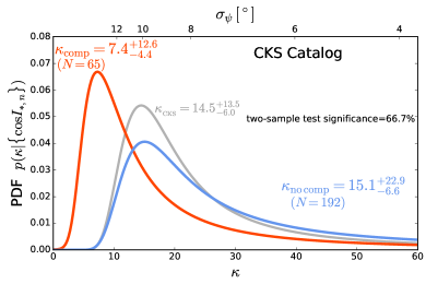
Figure 7.— Separation of the 257-target dataset into two subsets according to the presence ($N=65$) or absence ($N=190$) of stellar companions. Planet hosts with companions (red curve) appear to correspond to a lower value of $\kappa$ (a wider distribution of obliquities) than companionless systems (blue curve), but the statistical significance of this difference is negligible (it is $46\%$ likely to have happened by a random separation of the dataset).

Stellar Multiplicity

Another interesting property that can affect the obliquity of Kepler systems is stellar multiplicity. Different proposed channels for the origins of hot Jupiters (see Dawson & Johnson, 2018, for a recent review) typically invoke the presence of a distant companion of stellar or planetary mass that triggers the Lidov-Kozai mechanism or some related secular process responsible for high-eccentricities (e.g. Naoz, 2016). Some of these studies have explicitly provided predictions on the distribution of obliquities generated (see, e.g., Fabrycky & Tremaine, 2007; Naoz et al., 2012; Petrovich, 2015b, a; Anderson et al., 2016). However, moderate obliquities can be induced by a companion whether a system harbors a hot Jupiter or not, and these companions are not required to be in highly inclined orbits (e.g. Bailey et al., 2016; Lai, 2016; Lai et al., 2018). To test this, we use the adaptive optics follow-up observations of Furlan et al. (2017). This campaign – part of the Kepler Follow-up Observation Program KFOP (see Section 3.1.5 below – observed 3357 KOI host stars, reporting on the detection of 2297 companions to 1903 stars. Of the 773 KIC stars in the CKS catalog with confirmed planets (Section 3.1), 766 were part of the observation log of Furlan et al. (2017), including all of the 257 targets used in the present work. Using the results of the high-resolution imaging campaign of Furlan et al. (2017), we assign companion numbers to our 257 CKS targets. We find that 65 KOIs have one or more stellar companion candidates. Of these, 9 have $I_{*}\neq 90^{\circ}$ at a statistically significant level. As before, we split the dataset according to the presence of companions and carry out the concentration inference for each subsample.  In Fig. 7 (top panel) we show the posterior PDFs corresponding to each subset, finding that $\kappa^{\text{\tiny CKS}}_{\rm comp}=7.4^{+12.6}_{-4.4}$ and $\kappa^{\text{\tiny CKS}}_{\text{no comp}}=15.1^{+22.9}_{-6.6}$. Although the $\kappa$ posteriors appear somewhat distinguishable, the statistical significance of this difference is negligible, as the synthetic distance metric $\delta_{\mathrm{H}^{2}}$ was larger than the measured one in $\sim 35\%$ of the random data splittings attempted. The undetected effect of stellar multiplicity on obliquity might not be a surprise. The majority of these companions are detected beyond separation of $1.5^{\prime\prime}$, which in most cases (assuming a mean distance of $\sim 500$ pc) corresponds to 750 AU, a separation that might be too wide for a significant obliquity to accumulate due to differential precession over the age of the system (see, e.g., Boué & Fabrycky, 2014, and the Discussion below). Note that we have removed 34 targets with close companions for being possible blends that can make the period detection ambiguous (Section 3.1). We have repeated the obliquity inference reinstating these KOIs to see if they enclose some tentative clues regarding the influence of companions. Again, the $\kappa$ posteriors of the “companions” and ”no companions” subsamples are statistically indistinguishable.

Since the size of the sample allows us to split the dataset according to more than one variable, we have also explored planet multiplicity in combination with stellar multiplicity. No convincing trends arise, although some multis seem misaligned at a statistically significant level. This is the case KOI 377 (3 transiting planets) and KOI 1486 (2 transiting planets), for which the 95$\%$-confidence upper limits on $\cos I_{*}$ are 0.108 and 0.143, respectively (see caption in Fig. 3). This might seem counterintuitive at first, since the presence of additional planets could protect the system against external perturbations (e.g. Boué & Fabrycky, 2014; Lai & Pu, 2017; Lai et al., 2018). However, multi-planet systems could still shield each other from the excitation of mutual inclinations, while still being coherently inclined with respect to the stellar spin axis. The precise balance between external excitation and suppression of inclinations depends on all semi-major axes and masses of a given system, and thus any distinction between oblique and non-oblique populations might be much more subtle than what we have attempted here.

3.1.4 Obliquity Trends: Planetary Properties

As an initial test, in Section 3.1.2 we explored the role of planet multiplicity. However, we can explore other planetary properties such as orbital period and planet radius.

Orbital Period

Under the tidal-evolution hypothesis of Winn et al. (2010) and Albrecht et al. (2012), stellar obliquity should exhibit some dependence on planetary orbital period $P_{\rm orb}$. Using the photometric amplitude as an indicator of mean obliquity, Mazeh et al. (2015) concluded that low obliquities around cooler KOIs can extended out to $\sim 50$ days. However, using the same dataset, Li & Winn (2016) argue that the evidence for spin-orbit alignment partially weakens for $P_{\rm orb}\gtrsim 10$ days, and that it disappears when $P_{\rm orb}\gtrsim 30$ days. In Fig. 8 (top panel), we show the splitting of the CKS dataset by the period of the closest-in planet reveals a difference between short-period systems and long-period ones. For a period cutoff of $P_{\rm orb,cut}=8.5$ days, we find that short-period systems are more spin-orbit aligned that long-period ones, and that the statistical significance of this difference is of $97.8\%$ (a $\lesssim$2.5-$\sigma$ detection). We remove the 5 targets that can be classified as hot Jupiters and repeat the statistical test (bottom panel of Fig. 8), obtaining a mild increase in the significance of the trend. Despite the small number of targets removed, this additional test is not superfluous, as these 5 targets are the best candidates to test the tidal realignment hypothesis of Winn et al. (2010) (see also Albrecht et al., 2012; Dawson, 2014). The fact that closer-in planets are, on average, more spin-orbit aligned with their host stars is in qualitative agreement with the tidal realignment-hypothesis; however, as noted by Li & Winn (2016), it is suspect that this trend still applies for the small-mass planets in the CKS survey (see Discussion).

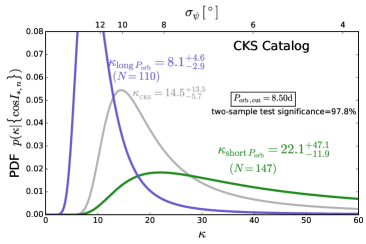
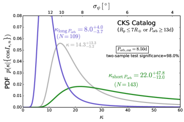
Figure 8.— Similar to figs. 6 and 7, this time separating the dataset by the orbital period of the closest-in planet. Top panel: separation of the entire 257-target into shorter-period systems ($P_{\rm orb}\leq 8.5$ d) and longer-period systems ($P_{\rm orb}>8.5$ d), producing $\kappa^{\text{\tiny CKS}}_{{\rm long}\,P_{\text{\tiny orb}}}=8.1^{+4.6}_{-2.9}$ (more oblique) and $\kappa^{\text{\tiny CKS}}_{{\rm short}\,P_{\text{\tiny orb}}}=22.1^{+47.1}_{-11.9}$ (less oblique). Bottom panel: same as above, but after excluding the 5 targets that can be classified as hot Jupiter systems ($R_{\rm p}>7R_{\oplus}$ and $P_{\rm orn}<13$ d). The obliquity trends are unaffected after removing those targets, and there is a slight increase in the statistical significance of the difference between the two subsets. In this case, the gray curve corresponds to the total sample after removing the 5 hot Jupiter targets.

Planet Radius

For each KOI, we define three statistics: the radius of the closest-in planet $R_{\rm p,c}$, the mean planet radius $\bar{R}_{\rm p}$ and the radius of the largest planet $R_{\rm p}^{\rm(max)}$. As with the exploration of orbital period, we split the dataset along these three quantities, sweeping the cut value $R_{\rm p,cut}$ until we find a maximum in the statistical significance. The results of this exploration are presented in Fig. 9, where the five hot Jupiter systems have been excluded in all three tests. All data splitting tests provide a consistent trend: systems with larger planets are more oblique than systems with smaller planets. For the metrics $R_{\rm p,c}$ and $\bar{R}_{\rm p}$ (top and middle panels of Fig. 9), the statistical significance of this trend is $99.5\%$ ($\lesssim 3{-}\sigma$). The test suggests that systems containing planets larger than $\sim 3R_{\oplus}$ (i.e., Neptunes and sub-Saturns) have larger stellar obliquities. MW14 discussed the possibility of this trend being behind their reported dependence on planet multiplicity, as multiple-transiting systems tend to have smaller mean radius (e.g., Latham et al., 2011). This idea is supported by the fact that the planet multiplicity trend is not present in the CKS catalog (see Fig. 4), while the dependence on planet radius is substantial. In conjunction with the stellar metallicity trend (Fig. 6), the obliquity-planet radius trend appears to point toward a dependence on the total mass contained in planets, in turn a measure of the “dynamical temperature” of a system (e.g. Tremaine, 2015). As we do not have accurate mass estimates for most of the planets in this sample, we cannot confidently define a statistic for the total mass contained in planets; however, in the Discussion, we speculate on ways of approximately assigning a total planetary mass to each KOI.

We briefly comment on the “sweeping data slicing” that we implemented above (Sections 3.1.3 and 3.1.4 )in order to identify potential breaks in the obliquity distribution. This technique was necessary because, for the variables tested, we lack a hypothesis predicting a change in the distribution of obliquities at some critical value of the variable in question. In addition, these variables – such as metallicity, age, planet orbital period and planet radius – are continuous, as opposed to categorical – such at multiplicity or planet type – which makes the a priori identification of an adequate cutoff ambiguous.

The sweeping of cutoff values means that we are carrying $N$ different hypothesis tests, one for each time a new cutoff is tried and the dataset is split. For each test, the “null hypothesis” $\mathcal{H}_{0,n}$ ($n=1,..,N$) is that the two subsets resulting from the splitting are indistinguishable from each other; we look for the $n$-th cutoff for which we can reject the null hypothesis at some confidence level. If the properties of the obliquity dataset change abruptly at the $n$-th cutoff, then the $n$-th $p$-value will be much smaller than that of any of the other tests (as it would be expected to happen, say, at the Kraft break). Alternatively, the obliquity data could depend smoothly and monotonically on some of these continuous variables, in which case the $p$-value could be small, not only for one, but for many of the $N$ tests.

When such multiple tests are attempted, it is important to quantify whether the null hypothesis in a given one of them could be rejected “by chance” due to “$p$-hacking”. This is sometimes referred to as the “multiple comparisons problem” (e.g., Miller, 1981). Multiple strategies have been devised to correct for this effect, the most widely used being the Holm-Bonferroni method (Holm, 1979), which adjusts the $p$-values of each test based on the number $N$ of tests carried out. An obstacle in implementing this adjustment is the clear correlation of our $N$ tests and of their resulting $p$-values (e.g., Conneely & Boehnke, 2007). Given this difficulty, we stick to our Monte Carlo approach. This time, we compute statistical significance by comparing the distance metric $\delta_{n}$ resulting from the $n$-th cutoff to the distance metrics obtained from all cutoffs attempted; thus, we compare to $5000\times N$ distance metrics with varying cutoff, instead of 5000 metrics with a fixed cutoff. For example, in Fig. 6 (top panel), the distance metric of the data splitting according to a metallicity cutoff of [Fe/H]$=0.135$ is $\delta_{\rm H^{2}}=0.563$, which is larger than in $96.85\%$ of all Monte Carlo data splittings across all $N$ tests: thus, the “global $p$-value” is 0.0315 (up from a value of $1-0.979=0.021$ obtained with the previous test); this allows us to reject the null hypothesis (that there is no metallicity dependence) at an $\alpha=0.04$ level. We repeat this analysis for orbital period (Fig. 8, top panel), and find a global $p$-value of 0.0256 (up from $1-0.978=0.022$). Similarly, for the planet radius dependence (Fig. 9, top panel) we find a global $p$-value of 0.0093 (up from $1-0.995=0.005$). Therefore, after introducing the global $p$-value as a way of dealing with the multiple comparisons problem, the detection significance remains roughly unaltered.

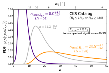
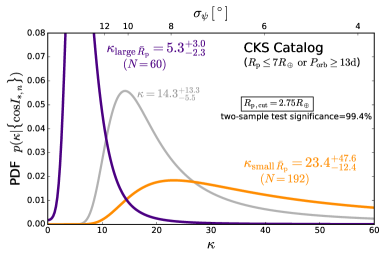
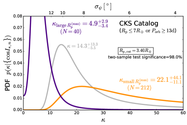
Figure 9.— Similar to Figs. 6-8, this time separating the CKS dataset (minus five hot Jupiter systems) by three different metrics related to the size of the planets in each system. Top panel: separation of the dataset by the radius of the closest-in planet $R_{\rm p,c}$, where the radius cut is placed at $R_{\rm p,cut}=2.75\,R_{\oplus}$; the large planet sample is more oblique on average with a concentration parameter $\kappa_{{\rm large}R_{\rm p}}=5^{+8.2}_{-0.5}$ and the small planet sample is less oblique with $\kappa_{{\rm small}R_{\rm p}}=23.5^{+48.3}_{-12.5}$. Middle panel: separation of the dataset by $\bar{R}_{\rm p}$, the mean planet radius, with $R_{\rm p,cut}=2.75\,R_{\oplus}$; as before, the large planet sample is more oblique than the small planet sample: $\kappa_{{\rm large}R_{\rm p}}=5.3^{+3}_{-2.3}$ and $\kappa_{{\rm small}R_{\rm p}}=23.4^{+47.6}_{-12.4}$. Bottom panel: separation of the dataset by maximum planet radius in each KOI ${R}^{\rm(max)}_{\rm p}$, with $R_{\rm p,cut}=3.4\,R_{\oplus}$; the large planet sample is more oblique than the small planet sample: $\kappa_{{\rm large}R_{\rm p}}=4.9^{+2.9}_{-3.4}$ and $\kappa_{{\rm small}R_{\rm p}}=22.1^{+44.1}_{-11.1}$. The two-sample statistical significance is $99.5\%$ (almost 3-$\sigma$) for $R_{\rm p,c}$ and $\bar{R}_{\rm p}$, and $98\%$ for ${R}^{\rm(max)}_{\rm p}$.

3.1.5 Other Catalogs of $\,V\sin I_{*}$ Measurements

Spectroscopic studies in the literature can provide with additional values of $V\sin I_{*}$ and $R_{*}$ (e.g., see Buchhave et al., 2012; Hirano et al., 2012, 2014). However, the CKS has signified a major leap with respect to previous studies, not only because of the size of its sample, but because of the consistency and uniformity of its data collection and analysis. In general, we expect CKS to supersede any previously reported spectroscopic analyses. There are however, significant amounts of KOI data that are publicly available via KFOP (Furlan et al., 2017), which has compiled follow-up imaging and spectroscopy of a large number KOIs. From the CFOP database, and as of Feb 20th, 2018, we obtain 858 individual KOIs with reported values and uncertainties of $V\sin I_{*}$ and $R_{*}$ by one or more users. Whenever more than one value of either $V\sin I_{*}$ or $R_{*}$ is reported, we perform a weighted mean of the values and their uncertainties. This database overlaps with the CKS database on 505 targets. Unfortunately, these reported values are inconsistent – uploaded by different users, using different rotational broadening fitting methods, applied on spectra obtained from different telescopes – and often the secondary by-product of a different type of analysis. Although some consistency is found between CFOP and CKS (rotational velocities tend to agree for $V\sin I_{*}<5\,$km s^-1, albeit with significant scatter), the accuracy and uniformity needed for the statistical analysis in the present work make the CKS catalog the only source can be used with confidence.

3.2. The TEPCat Catalog

The same kind of hierarchical Bayesian inference can be carried out for a database of projected obliquity measurements via use of Eq. (5). Using an essentially equivalent method, Fabrycky & Winn (2009) inferred a value of $\kappa$ from a list of 11 targets with RM observations. Using their sample, but implementing the formalism summarized in Section 2, we obtain $\kappa_{\text{\tiny~{}FW}}=9.1_{-7.1}^{+69}$, in consistency with the results of that work.

We can extend the same analysis to a much larger RM database. We retrieve the data compiled in John Southworth’s TEPCat Catalog (Southworth, 2011, http://www.astro.keele.ac.uk/jkt/tepcat/). This catalog contains 191 measurements for 118 unique systems. For multiple entries, we take the weighted mean of the observations, provided that there is some consistency between the reported measurements; if discrepancies are found, we take the latest/most accurate measurement. The measurement posterior of $\lambda$ for each target, i.e., $p(\lambda|\tilde{D}_{n})$ in Eq. 8, is taken to be a Gaussian with mean and variance given by each measurement and its uncertainty, respectively. The likelihood of the data given $\kappa$ is obtained via Eqs. (6) and (8), and the same prior (Eq.9) used in Section 3.1. The posterior PDF of $\kappa$ is shown in Fig. 10, and the $68\%$ probability interval is given by $\kappa_{\text{\tiny TEPCAT}}=2.2^{+0.2}_{-0.6}$. This value of the concentration parameter is much smaller than that obtained for the CKS sample, and corresponds to a much more oblique population ($\kappa=2$ implies $\langle\psi\rangle=53^{\circ}$ and $\sigma_{\psi}=30^{\circ}$). This discrepancy, however, is to be expected, as RM measurements are typically limited to hot Jupiter systems (Gaudi & Winn, 2007), in contrast to the more diverse nature of the Kepler exoplanet systems (see, e.g., Albrecht et al., 2012; Winn et al., 2017).

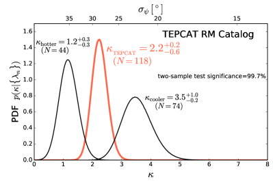
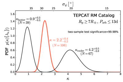
Figure 10.— Posterior PDF of the $\kappa$ parameter using RM data from the TEPCat catalog (Southworth, 2011). The posterior $p(\kappa|{\lambda_{n}})$ (red curve) is obtained from the multiplication of Eq. 6 by Eq. 9 using Eq. 8). Top panel: The concentration parameter of the entire TEPCat sample (118 objects) is $\kappa_{\text{\tiny TEPCAT}}=2.2^{+0.2}_{-0.6}$ (i.e., $\langle\psi\rangle\approx 53^{\circ}$ and $\sigma_{\psi}\approx 30^{\circ}$). The dataset can be divided into hotter and cooler subsamples ($T_{\rm eff}$ above and below 6250 K) with the hotter sample being more oblique (lower value of $\kappa$) by a statistically significant amount (3-$\sigma$ detection). Bottom panel: same as above, but for those targets in the TEPCat catalog for which $R_{\rm p}>7R_{\oplus}$ and $P_{\rm orb}\leq 13$ d (106 objects). In this case, $\kappa_{\text{\tiny TEPCAT,\,HJ}}=2.2^{+0.4}_{-0.2}$. The splitting of the dataset according to temperature produces $\kappa^{\text{ \tiny TEPCAT,\,HJ}}_{\rm hotter}=0.9\pm 0.3$ and $\kappa^{\text{ \tiny TEPCAT,\,HJ}}_{\rm cooler}=4.2^{+0.5}_{-0.8}$, with the difference being significant at the 4-$\sigma$ level.

Effective Temperature

The size of the TEPCat catalog allows us to split the dataset into subsamples. This is shown in Fig. 10 (top panel), where concentration inference was carried out for a “hotter” ($T_{\rm eff}\geq 6250$ K) subset with $N=44$ entries, and a “cooler” ($T_{\rm eff}<6250$ K) subset with $N=74$ entries. We find that $\kappa^{\text{ \tiny TEPCAT}}_{\rm hotter}=1.2\pm 0.3$ and $\kappa^{\text{ \tiny TEPCAT}}_{\rm cooler}=3.5^{+1}_{-0.2}$ with a statistical significance of $99.7\%$. Although the TEPCat catalog is largely composed on hot Jupiters, not all of its entries qualify as such. Indeed, if we only select targets with $R_{\rm p}>7R_{\oplus}$ and $P_{\rm orb}\leq 13$ d, we remove 12 targets. Repeating the separation of the dataset according to $T_{\rm eff}$ (Fig. 10, bottom panel), we find $\kappa^{\text{ \tiny TEPCAT,\,HJ}}_{\rm hotter}=0.9\pm 0.3$ and $\kappa^{\text{ \tiny TEPCAT,\,HJ}}_{\rm cooler}=4.2^{+0.5}_{-0.8}$, and that the hotter sample and the cooler sample are different with a $99.98\%$ statistical significance (almost a 4-$\sigma$ detection).

This obliquity-temperature dependence is in accordance to the confirmed trend that hotter hot Jupiter hosts tend to be more oblique cooler ones (Schlaufman, 2010; Winn et al., 2010; Hébrard et al., 2011; Albrecht et al., 2012; Dawson, 2014; Mazeh et al., 2015). Nevertheless, these values of $\kappa$ indicate that hot Jupiters systems are in general more oblique ($\kappa^{\text{ \tiny TEPCAT}}_{\rm cooler}\sim 4.2$) than the majority of configurations found in the Kepler catalog ($\kappa_{\text{\tiny CKS}}\sim 14$), regardless of stellar effective temperature. In principle, one could solely focus on hot Jupiters in the CKS sample to explore the discrepancy between $\kappa_{\text{\tiny~{}TEPCAT}}$ and $\kappa_{\text{\tiny~{}CKS}}$. Unfortunately, only 5/257 targets in the list compiled in Section 3.1 fall into the “hot Jupiter category” (see Section 4 below).

3.2.1 Three-dimensional Obliquities?

Having PDFs of both $\lambda$ and $\cos I_{*}$ can, in principle, be used to construct the three-dimensional obliquity $\psi$ (e.g. Benomar et al., 2014). The TEPCat and CKS databases overlap on 5 targets: KOI 377 (Kepler-9), KOI 203 (Kepler-17), KOI 806 (Kepler-30), KOI 63 (Kepler-63), KOI 94 (Kepler-89). Of these five targets, KOI-63 ($T_{\rm eff}=5673$ K) is severely oblique in both $\lambda$ and $I_{*}$, as already reported by Sanchis-Ojeda et al. (2013). KOI 63 is also unusual because it is one of the fastest rotators in the sample with $P_{\rm rot}=5.5$ days (the mean in the dataset is 18.8 days).

3.3. Obliquity Distribution of Hot Jupiters in the CKS and TEPCat Datasets

The significance of the temperature separation of the TEPCat sample is clear (Fig. 10). However, we lack the statistics to carry out an analogous test with the hot Jupiters in the CKS target list. The overall CKS sample used for our analysis ($N=257$) contains 20 stars above 6200 K ($7.8\%$). Of the 257 targets, only 5 are hosts to hot Jupiters, all below 6000 K. By contrast, $37\%$ of targets in the TEPCat catalog (mostly hot Jupiter hosts) have $T_{\rm eff}>6200$ K. This severely limits our ability to find a consensus between what can be inferred from RM measurements and via the $V\sin I_{*}$ method. Winn et al. (2017) found a workaround to this limitation, and using a statistical analysis of $V\sin I_{*}$ alone (e.g. Schlaufman, 2010), identified six systems above the Kraft break that are likely to be oblique: KOI 2, KOI 18, KOI 98, KOI 167, KOI 1117 and KOI 1852. None of these systems made it to our original 257-target dataset. KOI 98 was removed due to risk of blending and the other five have inconsistent SA and QPGP periods. The SA periods of KOIs 2, 18, 1117 and 1852 fall in a range of 60 to 90 days (very long for stars above the Kraft break, and likely to be wrong), while the corresponding QPGP periods are between 5 and 25 days, still somewhat long for these effective temperatures. If we use the QPGP periods for KOIs 2 (HAT-P-7), 18 and 1117 – $19.6\pm 4$, $24^{+12}_{-4}$ and $10\pm 1$ days respectively – we find that these KOIs have equatorial velocities $V_{\rm eq}\approx V\sin I_{*}$, and thus are consistent with $I_{*}\approx 90^{\circ}$. In this case, the low $V\sin I_{*}$ of these objects would result from them being anomalously slow rotators for their effective temperatures, and not from being highly oblique. On the other hand, the QPGP period of KOI 1852 ($6.9\pm 0.2$ days) does imply that this system could be severely oblique with $I_{*}(95\%)=50^{\circ}$, but it does not harbor a hot Jupiter. These estimates contradict some of the findings of Winn et al. (2017) in regard to the obliquity of hot Jupiter hosts above the Kraft break. It is interesting to note that KOI-2 (HAT-P-7) has already been reported to have either a polar or retrograde planetary orbit (Winn et al., 2009a). Thus, if indeed $\sin I_{*}\approx 1$ for this system, that could only be consistent with a fully retrograde configuration.

Whenever the SA and QPGP periods differ, it is typically when SA periods are extremely long. Some SA periods are longer than 100 days, while none of the QPGP periods are longer than 55 days. These extremely long periods could be an artifact of time series analysis or inherent to the Kepler instrumental systematics, which were never optimized to capture such long variability timescales (see Montet et al., 2017). Thus, in the absence of matching, if one rotational period is to be chosen, we favor those of Angus et al. (2018). A further advantage of these estimates is that the confidence intervals in $P_{\rm rot}$ of Angus et al. (2018) are the well-defined result of the Bayesian fitting of a parametric (albeit non-physical) model. If we use the QPGP for hot Jupiters, we increase the number of such objects in our database from 5 to 19. Under these circumstances, only four hot Jupiters are significantly oblique – KOIs 97, 127, 201 and 214 – of which only KOI 97 has $T_{\rm eff}>6000$ K. The upside of this exercise is that this list of 19 hot Jupiters is now marginally large enough for $\kappa$-inference. Our analysis results in $\kappa_{\text{\tiny HJ}}=0.01^{+11}_{-0.01}$, with a $\kappa$ posterior that is marginally distinguishable from the prior $\pi_{\kappa}$ (Eq. 9). If we instead use the prior $\pi^{\prime}_{\kappa}$ in Eq. (9b), which we may argue is a better representation of a Jeffreys prior at large $\kappa$, we find $\kappa_{\text{\tiny HJ}}=4^{+33}_{-3.9}$. It is difficult to conclude something from these results alone, but these concentration parameters cannot rule out that $\kappa_{\text{\tiny TEPCAT}}\approx 2.2$ provides an adequate representation of the underlying obliquity distribution of hot Jupiters.

4. Discussion

We have explored the influence of seven different variables on the obliquity concentration parameter using two publicly available catalogs of exoplanet systems: the CKS survey and the TEPCat catalog. The variables tested fall into the “stellar properties” category: (1) stellar effective temperature, (2) stellar age, (3) stellar metallicity and (4) stellar multiplicity; or into the “planetary properties” category: (5) planet multiplicity, (6) planet orbital period and (7) planet radius. From the CKS survey, we have found that metallicity, planet orbital period and planet radius are the variables to which obliquity is the most sensitive, while effective temperature is not testable using this catalog. Planet multiplicity, on the other hand, is found to have no significant correlation with stellar obliquity. The TEPCat catalog is used to find a very strong correlation with effective temperature, in agreement with similar previous claims in the literature.

In particular, exploration of three of those seven variables, namely $T_{\rm eff}$, stellar multiplicity and planet multiplicity, was motivated by previous observational and theoretical studies. All these three tests returned null results in the CKS catalog: those variables do not correlate with stellar obliquity.

The obliquity dependence on stellar effective temperature for hot Jupiters is the most robust of the trends found in the literature. Unfortunately, the $V\sin I_{*}$ method is not very effective at probing this relation, since the sample of KOIs with both $V\sin I_{*}$ and $P_{\rm rot}$ measurements is sparse above 6000 K. Hotter stars tend to be more variable and are also larger/brighter, and thus typically only large planets around the quietest of these stars can be detected (Mazeh et al., 2015; Winn et al., 2017). In turn, stars with little variability cannot be used to infer rotational periods via photometric modulation (McQuillan et al., 2014; Angus et al., 2018). We have attempted several approaches to isolate the hot Jupiter sample and study its obliquity properties, but more data are needed to robustly compute a value of $\kappa$ that can be compared to the one derived from TEPCat data. An alternative use of Kepler data to infer $I_{*}$ is asteroseismology, as done by Campante et al. (2016). This method represents a powerful alternative and complement to the $V\sin I_{*}$ method when stellar activity is too low to enable $P_{\rm rot}$ measurements, in turn permitting a reliable computation of the power spectrum of non-radial oscillations (e.g. Chaplin et al., 2011). Unfortunately, the 25-target list of Campante et al. (2016) contains only one hot Jupiter –KOI 2, which is oblique and above the Kraft break– not allowing us to address the temperature-obliquity relation reported by Winn et al. (2010). The fact that, by contrast, we find such a strong detection of temperature dependence in the TEPCat dataset (a 4-$\sigma$ detection, see Fig. 10) highlights the fact that the CKS and TEPCat catalog are, in general, probing different planet populations.

A dependence of $\kappa$ on stellar multiplicity could be detectable in similar datasets, provided that we can identify companions in an adequate manner and that these are close enough to induce obliquity through cumulative differential precession (e.g., Boué & Fabrycky, 2014). As we cannot know if the visual companions of Furlan et al. (2017) are truly bound, and we have removed some of the closest to avoid confusion due to blending, the true effect of stellar multiplicity in the Kepler sample remains unknown. Perhaps future missions of nearby planet-hosts such as TESS, complemented with astrometric information from Gaia (e.g., see Quinn & White, 2016), will not only improve our $\cos I_{*}$ estimates, but also help identify truly bound multiple stellar systems. In our analysis, we find that some multi-planet systems with companions show significant spin-orbit misalignment (in particular KOIs 377 and 1486, which drive the measured low value of $\kappa$ for this sub-population). It is possible that multi-planet systems are more susceptible to external torquing as they have a large collective quadrupole moment; provided that the multi-planet system is able to react nearly rigidly to external perturbations, the entire coplanar system can precess around the global angular momentum vector at a much faster rate than the host star would. (e.g., Kaib et al., 2011; Boué & Fabrycky, 2014). This process introduces an obliquity, which will depend on the mass, separation and inclination of the stellar companion (e.g., Lai, 2016).

The tentative dependence on planet multiplicity (MW14) is attractive as it fits into a picture of exoplanet statistics in which systems can be categorized according to their “dynamical temperature” (e.g. Tremaine, 2015): multi-planet systems are “dynamically cold”, having low mutual inclinations and near-zero eccentricities; “dynamically hot” systems, on the other hand, contains fewer planets and have larger eccentricities and mutual inclinations (Xie et al., 2016; Zhu et al., 2018). However, it is known that single-transiting systems are not necessarily true single-planet systems (Tremaine & Dong, 2012); indeed, Zhu et al. (2018) found that an important fraction of these observed singles exhibit signs of transit-timing variations (TTVs). Thus, even as a scrambled distribution of stellar obliquities would be consistent with dynamically hot systems, identifying which systems in our KOI sample are truly hot is difficult without measured eccentricities and/or TTVs. Unfortunately, we have not found any evidence to support this hypothesis by looking at planetary multiplicity alone.

Three variables appear to exhibit substantial to significant trends in the CKS catalog: stellar metallicity ($97.9\%$ significance), planet orbital period ($98\%$ significance) and planet radius ($99.5\%$ significance). The dependence on both stellar metallicity (Fig. 6) and planet radius (Fig. 9) could be pointing toward an underlying dependence on total mass contained in planets $M_{\rm p,tot}$, or the total orbital angular momentum contained in planets $\mathbf{J}_{\rm p,tot}$, probing the dynamical temperature of planetary systems in a more meaningful way than (observed) planet multiplicity alone. The total mass contained in planets $M_{\rm p,tot}$ is difficult do estimate from the current dataset. Even using the empirical mass-radius relation of Weiss & Marcy (2014), we still need to leave out 32 system for which that relation is not valid (systems with one or more planets with $R_{\rm p}<4R_{\oplus}$). If we simply label those 32 systems as “heavy” planetary systems and the rest as “light” ones, we indeed get a difference in the concentration parameter that is significant with a $98\%$ confidence. In the future, better planet mass estimates could shed light on the role of $M_{\rm p,tot}$ and $\mathbf{J}_{\rm p,tot}$ on the obliquity of the stellar host.

The dependence on planet orbital period is intriguing, especially because it seems to hold for planets of any mass. The work of Mazeh et al. (2015) suggest that some level spin-orbit alignment can even extend out to orbital periods of $\sim 50$ (our dataset contains only 15 KOIs for which the shortest orbital period is greater than 50 days). It is difficult to picture a scenario in which low-mass planets are able to modify the obliquity of their host star out to orbital periods of 10 days, let alone 50. Such planets cannot effectively torque the star as the total angular momentum contained in the planetary orbit is too small compared to that contained in stellar spin (e.g. Dawson, 2014), and thus this finding presents a severe challenge to proposed mechanisms of tidal realignment (e.g. Li & Winn, 2016). An alternative idea, proposed by Matsakos & Königl (2015) is that spin-orbit re-alignment can be achieved by planet ingestions, and that low obliquities are the result of the incorporation of orbital angular momentum onto the star, bringing its spin closer to that of the (nearly coplanar) planetary system. Under this hypothesis, stars above the Kraft break are less susceptible to realignment because they are faster rotators. In principle, this hypothesis should produce a correlation between obliquity and stellar rotational period (for $T_{\rm eff}$ above and below 6000 K). Since we use rotational periods to infer obliquities, we refrain from searching from such a correlation at this moment, as it would produce biased results. However, we encourage future observational work aiming at independently measuring obliquities and rotational periods of planet hosts.

Yet another novel hypothesis to explain the relation between obliquity and orbital period is that these planets are simply born within a gas disk that is closely aligned with the stellar spin. This would require the innermost regions of protoplanetary disks ($r\lesssim 0.1$ AU) to be immune to any external mechanisms that act to induce misalignment respect to the stellar equator. In principle, this can be achieved by a protostellar analog to the Bardeen-Petterson (BP) effect (Bardeen & Petterson, 1975), in which viscous accretion disks can reach a warped steady-state geometry that transitions into of perfect spin-orbit alignment within some transition radius. The BP effect is the result of a competition between the nodal precession of test particle orbits at some frequency $\Omega_{p}$ and the rate at which material and angular momentum are resupplied via advection (Kumar & Pringle, 1985). To a very rough approximation, once can identify the BP transition radius $r_{\rm BP}$ with the distance at which precession and advection balance each other, i.e., when $\Omega_{p}\sim 1/(\alpha^{2}t_{\rm visc})$ (Papaloizou & Pringle, 1983; Kumar & Pringle, 1985), where $\alpha$ is the viscosity parameter and $t_{\rm visc}\sim\alpha^{-1}h^{-2}(r)P_{\rm orb}$ is the viscous time and $h$ is the disk aspect ratio. The precession rate due to a rapidly spinning star is proportional to the oblateness quadrupole moment $J_{2}M_{*}R_{*}^{2}$ and scales with orbital radius as $\propto r^{-7/2}$. Alternatively, a magnetized protostar for which the magnetic moment $\boldsymbol{\mu}$ and spin vector are misaligned can also induce precessional torques, which act at a rate proportional to $\mu^{2}$ and scale with radius as $\propto r^{-11/2}$ (Lai, 1999; Pfeiffer & Lai, 2004). Of these two effects, the magnetic torque seems to be the most efficient one, as Pfeiffer & Lai (2004) state that $r_{\rm BP}\sim 3r_{\rm in}\sim 10R_{*}$, where $r_{\rm in}\propto\mu^{4/7}$ is the is the magnetospheric truncation radius. On the other hand, for a rapidly spinning oblate star (say, rotating at a tenth of the breakup rate) the transition radius is smaller: $r_{\rm BP}\approx R_{*}(\tfrac{3}{2}J_{2}\alpha h^{-2})^{1/2}\sim\mathcal{O}(R_{*})$. Thus, young stars can, in principle, enforce the spin-orbit alignment of the surrounding disk out to a distance of a few $R_{*}$, while regions outside that radius would be subject to external torques or able to retain any primordial misalignments.

5. Summary

In this work, we have studied the obliquity distribution of exoplanet host stars, performing an estimation of the concentration parameter $\kappa$, which serves as a measure of how narrow/wide the distribution of obliquities is around/away from $\psi=0^{\circ}$. We have carried out this parameter estimation using a hierarchical Bayesian inference method (Hogg et al., 2010; Foreman-Mackey et al., 2014, MW14), which we have applied to two publicly available datasets. The first one, the CKS (Petigura et al., 2017; Johnson et al., 2017), helps constrain $\kappa$ from measurements/inference of the LOS inclination of the stellar spin angle $I_{*}$. The second dataset (TEPCat Southworth, 2011), provides measurements of the projected obliquity onto the plane of the sky $\lambda$, which can also be used to estimate $\kappa$ (Section 2). From these datasets, we can conclude:

• The CKS dataset of $V\sin I_{*}$ and $R_{*}$ provides us with a target list ($N=257$) with LOS inclination angles that are consistent with a concentration parameter of $\kappa_{\text{\tiny CKS}}=14.5^{+13.5}_{-6}$, larger than previously measured for Kepler systems (MW14 found $\kappa_{\text{\tiny MW}}=6.2^{+1.8}_{-1.6}$) and consistent with a mean obliquity of $\langle\psi\rangle=19^{\circ}$ and a standard deviation of $\sigma_{\psi}=10^{\circ}$.

• The TEPCat dataset of $\lambda$ measurements ($N=118$) is consistent with $\kappa_{\text{\tiny TEPCAT}}=2.2^{+0.2}_{-0.6}$, meaning that the class of systems probed by RM observations (typically hot Jupiters) follow a significantly wider distribution of obliquities than those probed by the Kepler telescope.

We have divided the CKS and TEPCat datasets into separate bins according to stellar and planetary properties. With the CKS catalog, we have explored stellar age, stellar metallicity, stellar multiplicity, planet multiplicity, planet orbital period and planet radius. With the TEPCat catalog, we have explored stellar effective temperature. Our findings are:

• Planet multiplicity does not affect stellar obliquity at a statistically significant level in Kepler systems, and the weak trend originally pointed out by MW14 has vanished. This finding is in agreement the recent results of Winn et al. (2017). Although it is still true that compact multi-planet systems have very low obliquities (e.g. Sanchis-Ojeda et al., 2012; Albrecht et al., 2013), the converse is not necessarily true for single systems of any period and planet radius. Hot Jupiter systems, which do tend to lack nearby neighbors (Steffen et al., 2012), also tend to have higher obliquities on average (e.g., Hébrard et al., 2008; Winn et al., 2009b; Triaud et al., 2010; Albrecht et al., 2013), but this property does not extend to single-transiting systems with small planets.

• We have looked for trends in $\kappa$ as a function of stellar properties within the CKS set, exploring the dependence on $T_{\rm eff}$, stellar multiplicity, stellar age and stellar metallicity. The only obliquity trend that rises to a substantial statistical level ($\gtrsim 2.5{-}\sigma$) is that of metallicity. None of the other three stellar variables affects the inferred value of $\kappa$ above a 2-$\sigma$ level.

• A now well established trend is that hot Jupiters hosts with $T_{\rm eff}\gtrsim 6000$ K tend to be more oblique. This trend is impossible to probe with the CKS set (it lacks hot Jupiter systems with $T_{\rm eff}>6000$ K), but it is easily seen in the TEPCat catalog. By using concentration parameter inference on the TEPCat catalog, we have not only recovered a known temperature trend, but we have placed a quantitative measure of how much more oblique hotter hosts are. We find, when considering hot Jupiters alone (106 objects) $\kappa^{\text{ \tiny TEPCAT,HJ}}_{\rm hotter}=0.9\pm 0.3$ and $\kappa^{\text{ \tiny TEPCAT,HJ}}_{\rm cooler}=4.2^{+0.5}_{-0.8}$ with large statistical significance. Despite the greater obliquity of hot Jupiter host above the Kraft break, both concentration parameters $\kappa^{\text{ \tiny TEPCAT,HJ}}_{\rm hotter}$ and $\kappa^{\text{ \tiny TEPCAT,HJ}}_{\rm cooler}$ imply wide distributions of $\psi$. Thus, all hot Jupiters hosts in the TEPCat catalog are significantly more oblique than the overall Kepler systems, independently of the stellar effective temperature.

• We have looked for trends in $\kappa$ as a function of planetary properties within the CKS set. We find a trends with planetary orbital period at a substantial level ($2.5{-}\sigma$) period and a trend with planetary radius at a convincing level (${\sim}3{-}\sigma$). We propose the hypothesis that the correlation between obliquity and planet radius is indirectly probing a un underlying “dynamical temperature” trend. Under such hypothesis, the more tightly packed systems or those with higher total mass contained in planets will exhibit larger stellar obliquities. This is in accordance with the trend found with stellar metallicity. On the other hand, we propose that spin-orbit alignment in short-period systems is due to primordial alignment of the innermost protoplanetary gas disk, and not due to tidal realignment of the host star at later times.

• We have attempted to study the obliquity for hot Jupiters in the Kepler catalog. Given the small number of these objects for which all $V\sin I_{*}$, $R_{*}$ and $P_{\rm rot}$ can be compiled, it is difficult to provide a precise number. However, the data favors isotropic orientations over spin-orbit alignment, which is in rough agreement with the TEPCat results.

One of the remaining challenges when studying the statistical distribution of obliquity is being able to robustly measure the role of the Kraft break in stellar alignment. Although the $V\sin I_{*}$ method is observationally cheaper and less biased toward a specific type of planet than than RM observations, detecting small planets around stars with $T_{\rm eff}>6000$ K is difficult, as is the unambiguous identification of rotational periods. Of these two difficulties, perhaps the most concerning is the frequent lack of reliable periods for the hotter stars with detected planets (see Mazeh et al., 2015; Winn et al., 2017). The QPGP method of period identification seems promising when unveiling underlying rotational periods of active stars, although the possibility of significant differential rotation (e.g., Reiners, 2006) might require extensions to this parametric model. The identification of stellar $\sin I_{*}$ from future asteroseismological studies can be instrumental in providing an independent confirmation of the inference based on the $V\sin I_{*}$ approach.

We have provided open-source, documented software on how to carry out the hierarchical Bayesian inference of the concentration parameter $\kappa$. This software package has been made freely available online (github.com/djmunoz/obliquity_inference).

Appendix A Projected Obliquity

The three-dimensional orientation of the stellar spin vector can be written in terms of the polar and azimuthal angles $\theta$ and $\phi$ (Fabrycky & Winn, 2009; Morton & Winn, 2014) where the polar axis is $\hat{\mathbf{z}}$ – the unit angular momentum vector of the planetary orbit – or in terms of the angles $I_{*}$ and $\lambda$ (LOS-inclination and projected obliquity), in which the LOS vector $\hat{\mathbf{x}}$ plays the role of the polar axis. These two sets of angles are related by (see Eq. 2)

$$\cos I_{*}=\sin\theta\cos\phi~{}~{},$$ (A1a)

$$\sin I_{*}\sin\lambda=\sin\theta\sin\phi~{}~{},$$ (A1b)

$$\sin I_{*}\cos\lambda=\cos\theta~{}~{}.$$ (A1c)

Given the PDFs $f_{\theta}(\theta|\kappa)$ and $f_{\phi}(\phi)$, one can obtain the PDF $f_{\cos I_{*}}(\cdot|\kappa)$ using coordinate transformations (Morton & Winn, 2014, ; their equation 9). In a similar fashion, since $\tan\lambda=\tan\theta\sin\phi$ (Eqs. A1b-A1c), one can obtain a PDF for the quantity $\tan\lambda$ after obtaining the PDFs $f_{\tan\theta}(\cdot|\kappa)$ and $f_{\sin\phi}(\cdot|\kappa)$:

$$\begin{aligned} f_{\tan\theta}(y|\kappa)&=\frac{\kappa}{2\sinh\kappa}\frac{|y|}{(1+y^{2})^{3/2}}\exp\bigg{(}{\frac{\kappa}{\sqrt{1+y^{2}}}}\frac{y}{|y|}\bigg{)},~{}~{}~{}y\in(-\infty,\infty)\\ f_{\sin\phi}(x|\kappa)&=\frac{2}{\pi}\frac{1}{\sqrt{1-x^{2}}},\;\;\;\;x\in(0,1)\end{aligned}$$ (A2)

with $y=\tan\theta$ and $x=\sin\phi$. Combining these two expressions and using that

$$f_{\tan\lambda}(z|\kappa)=\int_{-\infty}^{\infty}f_{\tan\theta}(y|\kappa)f_{\sin\phi}(z/y~{}|\kappa)\frac{1}{|y|}dy~{}~{},$$ (A3)

we have, for $z=\tan\lambda$,

$$\begin{split}f_{\tan\lambda}(z|\kappa)&=\frac{\kappa}{\pi\sinh\kappa}{\times}\left\{\begin{array}[]{lc}\displaystyle\int\limits_{z}^{\infty}dy\frac{\exp({{\kappa}/{\sqrt{1+y^{2}}}})}{(1+y^{2})^{3/2}\sqrt{1-(z/y)^{2}}}&z>0\\ \displaystyle\int\limits_{|z|}^{\infty}dy\frac{\exp(-{{\kappa}/{\sqrt{1+y^{2}}}})}{(1+y^{2})^{3/2}\sqrt{1-(z/y)^{2}}}&z<0\end{array}\right.{=}\frac{\kappa}{\pi\sinh\kappa}\int\limits_{0}^{1/\sqrt{1+z^{2}}}d\tilde{y}\frac{\exp(\kappa\tilde{y}\,z/|z|)}{\sqrt{1-\tilde{y}^{2}}}\frac{\tilde{y}}{\sqrt{1-\frac{\tilde{y}^{2}}{1-\tilde{y}^{2}}z^{2}}}\end{split}$$ (A4)

This expression is valid in the range of $(0,\infty)$, and thus not very practical for random sampling purposes. However, using that $f_{\tan\lambda}|d\tan\lambda/d\lambda|=f_{\lambda}$, we can write:

$$\begin{split}f_{\lambda}(\lambda|\kappa)&=\frac{\kappa/\sinh\kappa}{\pi\cos^{2}\lambda}\int\limits_{0}^{\cos\lambda}d\tilde{y}\frac{\exp({{\kappa}\tilde{y}})}{\sqrt{1-\tilde{y}^{2}}}\frac{\tilde{y}}{\sqrt{1-\tan^{2}\lambda\tfrac{\tilde{y}^{2}}{1-\tilde{y}^{2}}}}\end{split}$$ (A5)

which we can confirm is correct by random sampling in $\theta$ and $\phi$ and computing the sampled values of $\lambda$ using Eq. A1 (see Fig. 11).

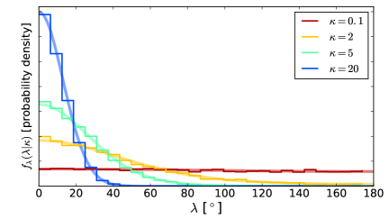
Figure 11.— PDF of $\lambda$ –the projected spin-orbit misalignment– given difference values of $\kappa$ (the Fisher concentration parameter) as given by Eq. (A5). Histograms are constructed after computing $\lambda$ from Monte Carlo samples ($N=2000$) of $\theta$ and $\phi$ (Eqs. A1b-A1c), where $\theta$ is sampled from the Fisher distribution in Eq. (3) and $\phi\sim U(0,\pi/2)$ .

Appendix B Background: Hierarchical Bayesian Inference of Meta-parameters

Here, we briefly describe the hierarchical Bayesian method introduced by Hogg et al. (2010). In this method, one seeks to carry out the estimation of the parameter vector ${\boldsymbol{\alpha}}$, which controls the probability distribution function (PDF) $f_{\boldsymbol{\omega}}(\boldsymbol{\omega}|{\boldsymbol{\alpha}})$ of a vector of physical quantities $\boldsymbol{\omega}$, which in turn contains the parameters $\{\omega_{i}\}$ of some parametrization of an individual object. With $N$ of such objects (in our case, exoplanet systems) the whole dataset $D$ can be split into subsets $D_{1},...,D_{N}$, with $D=\cup_{n=1}^{N}D_{n}$. By means of Bayes’ theorem, the posterior PDF of these “meta-parameters” ${\boldsymbol{\alpha}}$ for a given dataset $D$ is (Hogg et al., 2010)

$$\begin{split}p({\boldsymbol{\alpha}}|D)&\propto\mathcal{L}_{{\boldsymbol{\alpha}}}(\{D_{n}\}_{n=1}^{N}|{\boldsymbol{\alpha}})\,\pi_{\boldsymbol{\alpha}}({\boldsymbol{\alpha}})\\ &=\left[\prod_{n=1}^{N}p(D_{n}|{\boldsymbol{\alpha}})\right]\,\pi_{\boldsymbol{\alpha}}({\boldsymbol{\alpha}})\\ &\equiv\left[\prod_{n=1}^{N}\mathcal{L}_{{\boldsymbol{\alpha}},n}\right]\,\pi_{\boldsymbol{\alpha}}({\boldsymbol{\alpha}})~{}~{},\end{split}$$ (B1)

where $\mathcal{L}_{{\boldsymbol{\alpha}}}$ is the global likelihood, $\mathcal{L}_{{\boldsymbol{\alpha}}}$ is the likelihood associated to dataset $D_{n}$ and $\pi_{\boldsymbol{\alpha}}$ the prior information of the parameter vector ${\boldsymbol{\alpha}}$.

Instead of computing $\mathcal{L}_{{\boldsymbol{\alpha}},n}(D_{n}|{\boldsymbol{\alpha}})$ directly from the global dataset, this hierarchical method introduces a middle step, which is played by the vector of parameters per object ${\boldsymbol{\omega}}_{n}$, for which we already have previously computed posterior PDF obtained from its corresponding dataset $D_{n}$:

$$p({\boldsymbol{\omega}}_{n}|D_{n})=\frac{1}{Z_{n}}p(D_{n}|{\boldsymbol{\omega}}_{n})\pi_{{\boldsymbol{\omega}},0}({\boldsymbol{\omega}}_{n})$$ (B2)

where $Z_{n}$ is a normalization constant and $\pi_{{\boldsymbol{\omega}},0}$ is the (uninformative) prior for the vector of parameters ${\boldsymbol{\omega}}$. Then, one can write (Hogg et al., 2010; Foreman-Mackey et al., 2014)

$$\begin{split}\mathcal{L}_{{\boldsymbol{\alpha}},n}&=\int d{\boldsymbol{\omega}}_{n}p(D_{n}|{\boldsymbol{\omega}}_{n})p({\boldsymbol{\omega}}_{n}|{\boldsymbol{\alpha}})\\ &=Z_{n}\int d{\boldsymbol{\omega}}_{n}\frac{p({\boldsymbol{\omega}}_{n}|D_{n})}{\pi_{{\boldsymbol{\omega}},0}({\boldsymbol{\omega}}_{n})}p({\boldsymbol{\omega}}_{n}|{\boldsymbol{\alpha}})\end{split}$$ (B3)

The PDFs in Equations (4) and  (5) can replace $p({\boldsymbol{\omega}}_{n}|{\boldsymbol{\alpha}})$ in Eq. (B3) –with the parameter vectors ${\boldsymbol{\omega}}_{n}$ and ${\boldsymbol{\alpha}}$ having only one element each – to carry out the hierarchical inference calculation on $\kappa$.

Ignoring the normalization constant, $\mathcal{L}_{{\boldsymbol{\alpha}},n}$ can be interpreted as the distribution-weighted average of the ratio $p({\boldsymbol{\omega}}_{n}|{\boldsymbol{\alpha}})/\pi_{{\boldsymbol{\omega}},0}({\boldsymbol{\omega}}_{n})$, which allows for a Monte-Carlo approximation via $K-$sampling (Hogg et al., 2010)

$$\mathcal{L}_{{\boldsymbol{\alpha}},n}=\left\langle\frac{p({\boldsymbol{\omega}}_{n}|{\boldsymbol{\alpha}})}{\pi_{{\boldsymbol{\omega}},0}({\boldsymbol{\omega}}_{n})}\right\rangle_{{{\boldsymbol{\omega}}_{n}}}\approx\frac{1}{K}\sum\limits_{k=1}^{K}\frac{p({\boldsymbol{\omega}}_{n,k}|{\boldsymbol{\alpha}})}{\pi_{{\boldsymbol{\omega}},0}({\boldsymbol{\omega}}_{n,k})}$$ (B4)

where ${\boldsymbol{\omega}}_{n,k}$ is the $k$-th random sample of ${\boldsymbol{\omega}}_{n}$ obtained from the posterior $p({\boldsymbol{\omega}}_{n}|D_{n})$. Although very powerful, the $K$-sampling approximation is only justified for high-dimension integrals (as in the 7-variable case of Hogg et al., 2010). For the one-dimensional integrals of interest here (see below), $K$-sampling is not necessary and we instead use direct numerical integration.

References

- Aigrain et al. (2015) Aigrain, S., Llama, J., Ceillier, T., et al. 2015, MNRAS, 450, 3211
- Albrecht et al. (2011) Albrecht, S., Winn, J. N., Carter, J. A., Snellen, I. A. G., & de Mooij, E. J. W. 2011, ApJ, 726, 68
- Albrecht et al. (2013) Albrecht, S., Winn, J. N., Marcy, G. W., et al. 2013, ApJ, 771, 11
- Albrecht et al. (2012) Albrecht, S., Winn, J. N., Johnson, J. A., et al. 2012, ApJ, 757, 18
- Anderson et al. (2016) Anderson, K. R., Storch, N. I., & Lai, D. 2016, MNRAS, 456, 3671
- Angus et al. (2018) Angus, R., Morton, T., Aigrain, S., Foreman-Mackey, D., & Rajpaul, V. 2018, MNRAS, 474, 2094
- Bailey et al. (2016) Bailey, E., Batygin, K., & Brown, M. E. 2016, AJ, 152, 126
- Bardeen & Petterson (1975) Bardeen, J. M., & Petterson, J. A. 1975, ApJ, 195, L65
- Beck & Giles (2005) Beck, J. G., & Giles, P. 2005, ApJ, 621, L153
- Benomar et al. (2014) Benomar, O., Masuda, K., Shibahashi, H., & Suto, Y. 2014, PASJ, 66, 94
- Bonomo & Lanza (2012) Bonomo, A. S., & Lanza, A. F. 2012, A&A, 547, A37
- Borucki & Summers (1984) Borucki, W. J., & Summers, A. L. 1984, Icarus, 58, 121
- Boué & Fabrycky (2014) Boué, G., & Fabrycky, D. C. 2014, ApJ, 789, 111
- Buchhave et al. (2012) Buchhave, L. A., Latham, D. W., Johansen, A., et al. 2012, Nature, 486, 375
- Buzasi et al. (2016) Buzasi, D., Lezcano, A., & Preston, H. L. 2016, Journal of Space Weather and Space Climate, 6, A38
- Campante et al. (2016) Campante, T. L., Lund, M. N., Kuszlewicz, J. S., et al. 2016, ApJ, 819, 85
- Carrington (1863) Carrington, R. C. 1863, Observations of the Spots on the Sun from November 9, 1853, to March 24, 1861, Made at Redhill (London: Williams & Norgate)
- Chaplin et al. (2011) Chaplin, W. J., Bedding, T. R., Bonanno, A., et al. 2011, ApJ, 732, L5
- Conneely & Boehnke (2007) Conneely, K. N., & Boehnke, M. 2007, American journal of human genetics, 81 6, 1158
- Dawson (2014) Dawson, R. I. 2014, ApJ, 790, L31
- Dawson & Johnson (2018) Dawson, R. I., & Johnson, J. A. 2018, ArXiv e-prints, arXiv:1801.06117
- Doyle et al. (1984) Doyle, L. R., Wilcox, T. J., & Lorre, J. J. 1984, ApJ, 287, 307
- Fabrycky & Tremaine (2007) Fabrycky, D., & Tremaine, S. 2007, ApJ, 669, 1298
- Fabrycky & Winn (2009) Fabrycky, D. C., & Winn, J. N. 2009, ApJ, 696, 1230
- Fisher et al. (1993) Fisher, N. I., Lewis, T., & Embleton, B. J. J. 1993, Statistical Analysis of Spherical Data (Cambridge University Press)
- Fisher (1953) Fisher, R. 1953, Proceedings of the Royal Society of London Series A, 217, 295
- Foreman-Mackey et al. (2014) Foreman-Mackey, D., Hogg, D. W., & Morton, T. D. 2014, ApJ, 795, 64
- Furlan et al. (2017) Furlan, E., Ciardi, D. R., Everett, M. E., et al. 2017, AJ, 153, 71
- García et al. (2014) García, R. A., Ceillier, T., Salabert, D., et al. 2014, A&A, 572, A34
- Gaudi & Winn (2007) Gaudi, B. S., & Winn, J. N. 2007, ApJ, 655, 550
- Giménez (2006) Giménez, A. 2006, ApJ, 650, 408
- Gizon & Solanki (2003) Gizon, L., & Solanki, S. K. 2003, ApJ, 589, 1009
- Hébrard et al. (2008) Hébrard, G., Bouchy, F., Pont, F., et al. 2008, A&A, 488, 763
- Hébrard et al. (2011) Hébrard, G., Ehrenreich, D., Bouchy, F., et al. 2011, A&A, 527, L11
- Hirano et al. (2012) Hirano, T., Sanchis-Ojeda, R., Takeda, Y., et al. 2012, ApJ, 756, 66
- Hirano et al. (2014) —. 2014, ApJ, 783, 9
- Hogg et al. (2010) Hogg, D. W., Myers, A. D., & Bovy, J. 2010, ApJ, 725, 2166
- Holm (1979) Holm, S. 1979, Scand. J. Statist., 6, 65
- Jeffreys (1961) Jeffreys, H. 1961, Theory of Probability, 3rd edn. (Oxford)
- Johnson et al. (2017) Johnson, J. A., Petigura, E. A., Fulton, B. J., et al. 2017, AJ, 154, 108
- Kaib et al. (2011) Kaib, N. A., Raymond, S. N., & Duncan, M. J. 2011, ApJ, 742, L24
- Kraft (1967) Kraft, R. P. 1967, ApJ, 150, 551
- Kumar & Pringle (1985) Kumar, S., & Pringle, J. E. 1985, MNRAS, 213, 435
- Lai (1999) Lai, D. 1999, ApJ, 524, 1030
- Lai (2016) —. 2016, AJ, 152, 215
- Lai et al. (2018) Lai, D., Anderson, K. R., & Pu, B. 2018, MNRAS, arXiv:1710.11140
- Lai & Pu (2017) Lai, D., & Pu, B. 2017, AJ, 153, 42
- Latham et al. (2011) Latham, D. W., Rowe, J. F., Quinn, S. N., et al. 2011, ApJ, 732, L24
- Li & Winn (2016) Li, G., & Winn, J. N. 2016, ApJ, 818, 5
- Matsakos & Königl (2015) Matsakos, T., & Königl, A. 2015, ApJ, 809, L20
- Mazeh et al. (2015) Mazeh, T., Perets, H. B., McQuillan, A., & Goldstein, E. S. 2015, ApJ, 801, 3
- McLaughlin (1924) McLaughlin, D. B. 1924, ApJ, 60, doi:10.1086/142826
- McQuillan et al. (2013) McQuillan, A., Aigrain, S., & Mazeh, T. 2013, MNRAS, 432, 1203
- McQuillan et al. (2014) McQuillan, A., Mazeh, T., & Aigrain, S. 2014, ApJS, 211, 24
- Miller (1981) Miller, R. 1981, Simultaneous statistical inference, Springer series in statistics (Springer-Verlag)
- Montet et al. (2017) Montet, B. T., Tovar, G., & Foreman-Mackey, D. 2017, ApJ, 851, 116
- Morton & Johnson (2011) Morton, T. D., & Johnson, J. A. 2011, ApJ, 729, 138
- Morton & Winn (2014) Morton, T. D., & Winn, J. N. 2014, ApJ, 796, 47
- Mulders et al. (2016) Mulders, G. D., Pascucci, I., Apai, D., Frasca, A., & Molenda-Żakowicz, J. 2016, AJ, 152, 187
- Mullally et al. (2015) Mullally, F., Coughlin, J. L., Thompson, S. E., et al. 2015, ApJS, 217, 31
- Nagasawa et al. (2008) Nagasawa, M., Ida, S., & Bessho, T. 2008, ApJ, 678, 498
- Naoz (2016) Naoz, S. 2016, ARA&A, 54, 441
- Naoz et al. (2012) Naoz, S., Farr, W. M., & Rasio, F. A. 2012, ApJ, 754, L36
- Nutzman et al. (2011) Nutzman, P. A., Fabrycky, D. C., & Fortney, J. J. 2011, ApJ, 740, L10
- Ohta et al. (2005) Ohta, Y., Taruya, A., & Suto, Y. 2005, ApJ, 622, 1118
- Papaloizou & Pringle (1983) Papaloizou, J. C. B., & Pringle, J. E. 1983, MNRAS, 202, 1181
- Paz-Chinchón et al. (2015) Paz-Chinchón, F., Leão, I. C., Bravo, J. P., et al. 2015, ApJ, 803, 69
- Petigura et al. (2017) Petigura, E. A., Howard, A. W., Marcy, G. W., et al. 2017, AJ, 154, 107
- Petigura et al. (2018) Petigura, E. A., Marcy, G. W., Winn, J. N., et al. 2018, AJ, 155, 89
- Petrovich (2015a) Petrovich, C. 2015a, ApJ, 805, 75
- Petrovich (2015b) —. 2015b, ApJ, 799, 27
- Pfeiffer & Lai (2004) Pfeiffer, H. P., & Lai, D. 2004, ApJ, 604, 766
- Pu & Wu (2015) Pu, B., & Wu, Y. 2015, ApJ, 807, 44
- Queloz et al. (2000) Queloz, D., Eggenberger, A., Mayor, M., et al. 2000, A&A, 359, L13
- Quinn & White (2016) Quinn, S. N., & White, R. J. 2016, ApJ, 833, 173
- Reiners (2006) Reiners, A. 2006, A&A, 446, 267
- Rossiter (1924) Rossiter, R. A. 1924, ApJ, 60, doi:10.1086/142825
- Sanchis-Ojeda et al. (2012) Sanchis-Ojeda, R., Fabrycky, D. C., Winn, J. N., et al. 2012, Nature, 487, 449
- Sanchis-Ojeda et al. (2013) Sanchis-Ojeda, R., Winn, J. N., Marcy, G. W., et al. 2013, ApJ, 775, 54
- Schatzman (1962) Schatzman, E. 1962, Annales d’Astrophysique, 25, 18
- Schlaufman (2010) Schlaufman, K. C. 2010, ApJ, 719, 602
- Soderblom (1985) Soderblom, D. R. 1985, PASP, 97, 57
- Southworth (2011) Southworth, J. 2011, MNRAS, 417, 2166
- Steffen et al. (2012) Steffen, J. H., Ragozzine, D., Fabrycky, D. C., et al. 2012, Proceedings of the National Academy of Science, 109, 7982
- Struve (1930) Struve, O. 1930, ApJ, 72, doi:10.1086/143256
- Tremaine (2015) Tremaine, S. 2015, ApJ, 807, 157
- Tremaine & Dong (2012) Tremaine, S., & Dong, S. 2012, AJ, 143, 94
- Triaud (2011) Triaud, A. H. M. J. 2011, A&A, 534, L6
- Triaud et al. (2010) Triaud, A. H. M. J., Collier Cameron, A., Queloz, D., et al. 2010, A&A, 524, A25
- Weiss & Marcy (2014) Weiss, L. M., & Marcy, G. W. 2014, ApJ, 783, L6
- Winn et al. (2010) Winn, J. N., Fabrycky, D., Albrecht, S., & Johnson, J. A. 2010, ApJ, 718, L145
- Winn & Fabrycky (2015) Winn, J. N., & Fabrycky, D. C. 2015, ARA&A, 53, 409
- Winn et al. (2009a) Winn, J. N., Johnson, J. A., Albrecht, S., et al. 2009a, ApJ, 703, L99
- Winn et al. (2007) Winn, J. N., Holman, M. J., Henry, G. W., et al. 2007, AJ, 133, 1828
- Winn et al. (2009b) Winn, J. N., Johnson, J. A., Fabrycky, D., et al. 2009b, ApJ, 700, 302
- Winn et al. (2017) Winn, J. N., Petigura, E. A., Morton, T. D., et al. 2017, AJ, 154, 270
- Xie et al. (2016) Xie, J.-W., Dong, S., Zhu, Z., et al. 2016, Proceedings of the National Academy of Science, 113, 11431
- Zhu et al. (2018) Zhu, W., Petrovich, C., Wu, Y., Dong, S., & Xie, J. 2018, ArXiv e-prints, arXiv:1802.09526