On the Interpretation of Far-infrared Spectral Energy Distributions. I: The 850 $\mu$m Molecular Mass Estimator

Abstract

We use a suite of cosmological zoom galaxy formation simulations and dust radiative transfer calculations to explore the use of the monochromatic $850~{}\mu m$ luminosity (L_ν,850) as a molecular gas mass (M_mol) estimator in galaxies between $0<z<9.5$ for a broad range of masses. For our fiducial simulations, where we assume the dust mass is linearly related to the metal mass, we find that empirical L_ν,850-M_mol calibrations accurately recover the molecular gas mass of our model galaxies, and that the L_ν,850-dependent calibration is preferred. We argue the major driver of scatter in the L_ν,850-M_mol relation arises from variations in the molecular gas to dust mass ratio, rather than variations in the dust temperature, in agreement with the previous study of Liang et al. Emulating a realistic measurement strategy with ALMA observing bands that are dependent on the source redshift, we find that estimating S_ν,850 from continuum emission at a different frequency contributes $10-20\%$ scatter to the L_ν,850-M_mol relation. This additional scatter arises from a combination of mismatches in assumed T${}_{\textnormal{\scriptsize{dust}}}$ and $\beta$ values, as well as the fact that the SEDs are not single-temperature blackbodies. However this observationally induced scatter is a sub-dominant source of uncertainty. Finally we explore the impact of a dust prescription in which the dust-to-metals ratio varies with metallicity. Though the resulting mean dust temperatures are $\sim 50\%$ higher, the dust mass is significantly decreased for low-metallicity halos. As a result, the observationally calibrated L_ν,850-M_mol relation holds for massive galaxies, independent of the dust model, but below L_ν,850 $\lesssim 10^{28}$ erg s^-1 (metallicities $\log_{10}({\rm Z}/{\rm Z}_{\odot})\lesssim-0.8$) we expect galaxies may deviate from literature observational calibrations by $\gtrsim 0.5$ dex.

1 Molecular Reservoirs in Galaxies and Thermal Dust Emission

Molecular gas has long been recognized as a key ingredient in galaxy evolution, largely through its consumption in star formation. Accordingly, determining the mass of molecular gas reservoirs, M_mol, has been pursued as an important property of galaxies. The most common method of constraining the molecular gas content of galaxies is via observations of low-J transitions of CO, and converting to an equivalent H₂ mass (e.g., Bolatto et al., 2013; Casey et al., 2014, and references therein).

Single-band continuum estimators of the molecular gas mass have been increasingly used to chart the evolution of the ISM content of galaxies at high redshift (e.g., Scoville et al., 2014; Groves et al., 2015; Scoville et al., 2016; Schinnerer et al., 2016; Scoville et al., 2017; Bertemes et al., 2018). The continuum sensitivity of the Atacama Large Millimeter Array (ALMA) means dust measurements can be obtained rapidly for high-z sources (e.g., Scoville et al., 2014). If these dust emission measurements can be reliably converted to molecular gas mass estimates, the sensitivity of ALMA would enable the study of the gas content of large samples of galaxies (e.g,. Scoville et al., 2016, 2017). Generally, this takes the form of:

$$L_{\nu}=CT_{\rm dust}\kappa_{\nu}\frac{M_{\rm dust}}{M_{\rm gas}}M_{\rm gas}=\Upsilon M_{\rm gas}$$ (1)

Where C is an unknown proportionality constant, and $\Upsilon$ is empirically calibrated from existing observations. We note that this approach differs from techniques which fit the full spectral energy distribution to derive M_dust and then assume a dust-to-gas ratio to estimate M_mol (e.g., Magdis et al., 2012).

In a series of papers Scoville et al. (2014, 2016) outlined a procedure for estimating molecular gas masses using long-wavelength continuum measurements, directly at $850~{}\mu m$ or by observing redshifted continuum emission from a higher-frequency rest-frame and down-converting it to $850~{}\mu m$. They additionally calibrated this relationship empirically against massive galaxies at $z=0$ and $z\sim 2$ which had both dust continuum ($850~{}\mu m$ or $500~{}\mu m$) and CO (1–0) measurements. A similar calibration was also derived by using Planck observations of Milky Way molecular clouds. Scoville et al. (2014) find a relationship of:

$$\frac{L_{\rm\nu,850}}{M_{\rm mol}}=\alpha_{\nu,850}=(6.7\pm 1.7)\times 10^{19}~{}({\rm erg}~{}{\rm s}^{-1}~{}{\rm Hz}^{-1}~{}\rm{M}_{\odot}^{-1})$$ (2)

Note that $\alpha_{\rm\nu,850}$ differs from $\Upsilon$ in Equation 1 because $\alpha_{\rm\nu,850}$ converts only to the molecular gas mass. To perform this empirical calibration based on the galaxy sample Scoville et al. (2014, 2016) assumed a CO to H₂ conversion factor of $\alpha=6.5$ M_⊙ $($K km s^-1 pc${}^{2})^{-1}$, including the contribution from He. Hughes et al. (2017) found a similar calibration using a sample of main sequence star forming galaxies across the redshift range $0.02<z<0.35$. Additionally, Janowiecki et al. (2018) explored the observational systematics in the L_ν,850-M_mol relation for galaxies in the volume-limited Herschel Reference Survey. The found that deviations from M_mol-dust emission relations primarily correlate with the H i/H₂ fraction.

Here we test the proportionality between the thermal dust emission and the molecular gas mass by using a suite of hydrodynamic cosmological zoom simulations spanning a redshift range of $0\leq z\lesssim 9.5$. These simulations are coupled with dust radiative transfer post-processing to explore the link between the dust emission and the galaxy molecular mass. The advantage of this approach is that the M_mol values derived from the synthetic L_ν,850 “measurements” (using the observationally derived $\alpha_{\rm\nu,850}$ conversion factor) can be directly compared with the molecular gas masses in the simulations. Discrepancies can be further correlated with the known dust temperature (T${}_{\textnormal{\scriptsize{dust}}}$), dust mass (M_dust), and molecular gas to dust mass of the galaxies in the simulations.

We begin by describing the cosmological zoom simulations and radiative transfer post-processing (Section 2), then apply the L_ν,850 mass estimation technique (Section 3), before comparing to the intrinsic properties of the simulations (Section 4), discussing the likely origins of scatter about the relationship (Section 5), and concluding with a brief discussion of the implications for high-redshift ALMA observations (Section 6.1). Throughout the paper we assume a Planck2013 cosmology ($H_{0}=67.77$ km s^-1 Mpc^-1, $\Omega_{\rm matter}=0.30713$; Planck Collaboration et al., 2014).

2 Numerical Methods

Our aim is to use modeled submillimeter-wave flux densities from galaxies at high-redshift to test how the dust continuum emission relates to the underlying molecular gas mass and test observational M_mol estimators. To do this, we will model a sample of simulated galaxies at high-redshift using the cosmological zoom technique, and from those generate the synthetic broadband SEDs. To do this, we will follow Olsen et al. (2017); Narayanan et al. (2018b) and Abruzzo et al. (2018), and combine galaxies zoomed in on from the mufasa cosmological simulation series (Davé et al., 2016, 2017a, 2017b) with powderday dust radiative transfer (Narayanan et al., 2015, 2018a). In this section, we will summarize these methods, though refer the readers to the aforementioned works (in particular Narayanan et al., 2018b) for further details.

2.1 Cosmological Zoom Galaxy Formation Simulations

We perform our galaxy formation simulations using the hydrodynamic galaxy formation code gizmo (Hopkins, 2015, 2017; Hopkins et al., 2017). These simulations are performed in meshless finite mass (MFM) mode, in which the cubic spline kernel is used to define the volume partition between gas elements (and, therefore, the faces over which the Riemann solver solves the hydrodynamic equations).

The cosmological zoom technique isolates dark matter halos of interest at a particular redshift, and re-simulates these at higher resolution. Functionally, we first initialize the simulation at $z=249$ using music (Hahn & Abel, 2011), where the initial conditions are identical to those in the mufasa cosmological simulations (Davé et al., 2016). We then run a run a coarse dark matter only simulation to $z=0$ with particle mass $7.8\times 10^{8}h^{-1}M_{\odot}$ in a $50h^{-1}$ Mpc volume, and $512^{3}$ dark matter particles. From this dark matter simulation, we select model halos to re-simulate at higher resolution, and with baryons included.

We identify these halos using caesar (Thompson et al., 2014), and track all particles that fall within $2.5\times r_{\rm max}$ of the halo of interest back to $z=249$. Here, $r_{\rm max}$ is the radius of the farthest particle from halo center; this technique, while computationally expensive, ensures that we have a $0\%$ contamination rate of low-resolution particles in our final model halos.

For the purposes of this paper, we analyze $7$ model halos over a broad range of final halo masses. We list some relevant physical properties of these halos in Table 1. The $4$ most massive halos are selected from a $z=2$ snapshot, and only run to $z_{\rm final}\approx 2$, while the remaining $3$ were selected from a $z=0$ snapshot (and consequently run to $z_{\rm final}\approx 0$). These model halos range from approximately Milky Way mass at $z=0$ to massive halos that may represent luminous dusty star forming galaxies at high-redshift (Casey et al., 2014).

Table 1: Zoom Simulation Summary

Halo ID	$z_{\rm final}$	MDM($z=2$)	M∗($z=2$)	M∗($z_{\rm final}$)
		($\times 10^{11}$ M⊙)	($\times 10^{10}$ M⊙)	($\times 10^{10}$ M⊙)
0	2.15	41.0	$\cdots$	10.50
5	2.05	63.0	$\cdots$	10.32
10	2.00	11.0	8.82	18.82
45	2.00	37.0	1.02	11.02
287	0.65	10.3	0.28	10.39
352	0.00	10.9	0.47	13.42
401	0.02	10.6	0.34	12.60

Note. — Halo ID number, final redshift of zoom simulation, total halo mass at $z=2$, stellar mass within a 50 kpc box at $z=2$, and stellar mass within a 50 kpc box at the final redshift.

The baryonic zoom galaxy formation simulations are run with the mufasa suite of physics Davé et al. (2016). In short, stars form in dense molecular gas according to a volumetric Schmidt (1959) relation, with an imposed star formation efficiency per free fall time of $\epsilon_{*}=0.02$, as motivated by observations (Kennicutt, 1998; Kennicutt & Evans, 2012; Narayanan et al., 2008, 2012; Hopkins et al., 2013). The molecular gas fraction is determined following Krumholz et al. (2009), wherein the molecular gas fraction is tied to the surface density of the gas, and its metallicity. The gas surface density is computed using the Sobolev approximation, as described in Davé et al. (2016) and uses kernel-smoothing of the nearest 64 neighbors. The mufasa cosmological simulations reproduce the observed $z=0$ H₂ mass function and $f_{H_{2}}-M_{*}$ relation (Davé et al., 2017b). When considering the H₂ to CO conversion of Narayanan et al. (2012), the mufasa simulations also reasonably reproduce the CO (1–0) luminosity function out to $z\sim 2$.

Alternate H₂ prescriptions exist, including a modified KMT model (Krumholz, 2013) and models dependent on the gas-to-dust ratio and interstellar radiation field (e.g., Gnedin & Kravtsov, 2011; Gnedin & Draine, 2014). Lagos et al. (2015) explored the differences of the Krumholz (2013) and Gnedin & Kravtsov (2011) models on the implied H₂ properties of the EAGLE simulation (Schaye et al., 2015). Popping et al. (2014) also explored pressure (Blitz & Rosolowsky, 2006) and metallicity-based (Gnedin & Kravtsov, 2011) H₂ prescriptions in semi-analytic models. Both studies found that the $z=0$ H₂ mass function was reasonably well reproduced by all the models. Discrepancies in H₂ masses between models were most significant in low-metallicity galaxies (Z$<0.5$Z_⊙; Lagos et al., 2015) or low mass halos (M${}_{\rm halo}<10^{10}$ M_⊙; Popping et al., 2014).

In principle, variations in H₂ could be explored for these zooms by re-evaluating them in post-processing and choosing an alternate sub-grid model. However, this would introduce inconsistencies in the analysis, compromising a fair comparison. Changes in the H₂ model would propagate to changes in the star formation histories, which in turn would affect the metallicity. The modified metallicity and star formation history would further result in changes in the dust masses and the dust temperatures. These changes are not straightforward to estimate and would obviate a clear interpretation of the impact of varying H₂ prescriptions, so we have not attempted to do so here. This is a problem which is likely best addressed with a future study running new suites of zoom simulations with different H₂ prescriptions to perform an internally consistent study.

We track the evolution of $11$ elements: H, He, C, N, O, Ne, Mg, Si, S, Ca and Fe. We draw SNe type 1a yields from Iwamoto et al. (1999), assuming $1.4M_{\odot}$ of mass returned into the ISM per supernova. Following Davé et al. (2016), type SNe type II yields are derived from the Nomoto et al. (2006) prescription, though we reduce these by $50\%$ in order to match mass-metallicity constraints at high-redshift (Davé et al., 2011). The dust yields from AGB stars derive from the Oppenheimer & Davé (2008) lookup tables.

Feedback from massive stars are included as a decoupled two phase wind scheme in the mufasa wind model. Here, the stellar winds have a probability for ejection that is a fraction of the star formation rate probability. This fraction derives from scaling relations from the Feedback in Realistic Environments project (Muratov et al., 2015; Hopkins et al., 2014, 2017). Here, the ejection velocity depends on the galaxy circular velocity, which is determined on the fly using a fast friends of friends finder. AGB and Type Ia supernovae winds are included, following Bruzual & Charlot (2003) tracks with a Chabrier (2003) initial mass function. These simulations broadly agree with observational constraints of the SFR-$M_{*}$ relation, and $M_{*}-M_{\rm halo}$ relation (Abruzzo et al., 2018)

2.2 Dust Radiative Transfer

With our model galaxies in hand, we now turn to generating their synthetic broadband SEDs. We do this using the publicly available powderday simulation package (Narayanan et al., 2015, 2018a), that wraps fsps for the stellar population synthesis (Conroy et al., 2009; Conroy & Gunn, 2010; Conroy et al., 2010) with yt for grid generation (Turk et al., 2011), and hyperion for dust radiative transfer (Robitaille, 2011; Robitaille et al., 2012).

Functionally, we cut a $50$ kpc box around the model central galaxy in each snapshot, and build an adaptive grid with an octree memory structure. We begin with one cell encompassing all gas particles in this box, and subdivide each cell into octs until a threshold number of particles $n_{\rm thresh}=64$ is reached in each cell.

The SEDs for the star particles within each cell are generated with fsps using the stellar ages and metallicities as returned from the cosmological simulations. For these, we assume a Kroupa (2002) stellar IMF and the Padova stellar isochrones (Marigo & Girardi, 2007; Marigo et al., 2008). These stellar SEDs provide the input spectrum that transfers through the dusty ISM of the galaxy.

For our fiducial simulations, the dust mass of each cell is assumed to be tied to the metal mass by a constant fraction: $M_{\rm dust}=0.4\times M_{\rm metal}$. This is motivated by observations of both local galaxies and those at high-redshift (Dwek, 1998; Vladilo, 1998; Watson, 2011; Sandstrom et al., 2013). We also briefly explore a prescription in which the dust-to-metals ratio is a smoothly varying function of the metallicity (Section 6.2, Appendix C), motivated by Rémy-Ruyer et al. (2014). In both cases, the dust is modeled as the carbonaceous-silicate Draine & Li (2007) model that follows the Weingartner & Draine (2001) size distribution, and the Draine (2003) renormalization relative to Hydrogen. We assume $R_{\rm V}\equiv A_{\rm V}/E\left(B-V\right)=3.15$. This dust is assumed to uniformly fill each cell. We have performed resolution studies to ensure that reducing $n_{\rm thresh}$ does not change our results appreciably. Unless otherwise noted, our discussions refer to the fiducial dust model. In this paper we use “metallicity” to refer to the total metals plus dust.

The radiation from the stars is propagated throughout the grid in $3$ dimensions using hyperion. The radiative transfer occurs in a Monte Carlo fashion, and employs the Lucy (1999) equilibrium algorithm to determine the equilibrium condition between the radiation field and dust temperature. In this process, we emit radiation from all of the stellar sources, and this radiation is absorbed, scattered, and remitted from each cell. We iterate on this process until the energy absorbed by $99\%$ of the cells has changed by less than $1\%$.

It is important to note that we do not include any sub-resolution models for birth clouds (e.g. Groves et al., 2004; Jonsson et al., 2010; Narayanan et al., 2010). The compactness and covering fraction of these birth clouds tends to be free parameters, and can have a significant impact on the final dust SED, depending on the final parameter choices. We discuss the impact of a birth cloud model in Appendix D.

New to these calculations (as compared to Narayanan et al., 2018b), we include the effects of the cosmic microwave background (CMB). As we will show, in some scenarios this can make an impact on our results (see also da Cunha et al., 2013). We include the CMB as an additional energy density term in each cell as the energy absorbed per unit dust mass in each cell (i.e. $\epsilon=\int\kappa_{\nu}B_{\nu}d\nu$ erg/s/g, where $\kappa_{\nu}$ is the dust absorption opacity, and $B_{\nu}$ is the Planck function). The CMB temperature is simply $T_{\rm CMB}=2.73(1+z)$ K, where $z$ is the redshift of the snapshot.

We note that the values for the radiative transfer parameters described thus far are constrained by observed data and we did not engage in any tuning of the treatment of dust properties in the simulations. The net result of our radiative transfer calculations is a broadband SED, from $\lambda=912$ Å–3 mm (3287 THz – 100 GHz). It is these SEDs that we analyze for the remainder of this paper.

In Figure 1 we show the evolution of the physical properties of each simulated halo, including the stellar mass (M_∗), molecular gas mass (M_mol) including He, atomic gas mass (M_atomic), dust mass (M_dust), molecular mass-weighted mean dust temperature($\langle T_{\rm dust}\rangle_{M}$), and mean gas phase metallicity weighted by the total gas mass ($\langle Z\rangle_{M}$). All quantities are computed inside a box 50 kpc across, centered on the center of mass of the central galaxy in the halo. The dust mass appears to broadly track M_mol and the metallicity, and is roughly independent of the atomic gas mass (here taken to include everything which is not in molecular form). The dust temperatures begin high ($\sim 30-50$ K), reflecting a combination of the intrinsic heating from star formation and low dust masses along with additional heating from the CMB (Appendix B), eventually decreasing to typical low-redshift values of $\sim 30$ K. In the remainder of the paper we explore the thermal continuum emission from the dust and compare it with M_mol, $\langle T_{\rm dust}\rangle_{M}$, $\langle Z\rangle_{M}$, and M_dust/M_mol, to assess the precision of L_ν,850 as an estimator for M_mol.

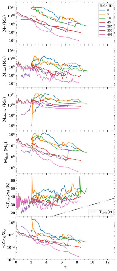
Figure 1: The evolution of various physical properties of the simulated galaxies, as directly measured from the snapshots and subsequent post-processing. From top to bottom: stellar mass (M_∗), molecular gas mass (M_mol) including He, atomic gas mass (M_atomic), dust mass (M_dust), molecular mass-weighted mean dust temperature($\langle T_{\rm dust}\rangle_{M}$), and mean gas phase metallicity weighted by the total gas mass ($\langle Z\rangle_{M}$). In the panel showing T${}_{\textnormal{\scriptsize{dust}}}$, the black dotted line shows the CMB temperature as a reference. All quantities in this and subsequent plots are computed within a 50 kpc by 50 kpc box centered on the center of mass of the most massive galaxy in the high-resolution dark matter halo.

3 Single-band Mass Indicators

Here we explore the application of the L_ν,850 mass estimator to the SEDs generated from the cosmological zoom simulations, using the same assumptions made for interpretation of observations. We seek to answer two questions:

1. Do we recover a close link between a galaxy’s intrinsic L_ν,850 and its molecular gas mass M_mol using these realistic simulations?

2. If there is a good L_ν,850-M_mol relation, what impact do realistic observing techniques, namely band-correction of fluxes, have on our ability to accurately recover M_mol?

To answer the first question we explore an ideal scenario where the rest-frame $850~{}\mu m$ emission can be measured to directly compute L_{ν,850,direct}, then converting this to a molecular mass using the Scoville et al. (2016) calibration (Section 3.1). This will directly probe the intrinsic link between the 850 $\mu$m continuum and M_mol.

To answer the second question we investigate a more observationally realistic case where observations performed are of emission with $\nu_{\rm rest}>\nu_{850}$. These observations must then be converted to an equivalent $850~{}\mu m$ flux by assuming optically thin emission, a dust emissivity index $\beta$, and a (mass-weighted) dust temperature, $\langle T_{\rm dust}\rangle_{\rm M}$ (Section 3.2). This latter approach results in an inferred luminosity, L_{ν,850,inferred}. Comparison of these two cases will enable us to separate any offsets introduced by the band conversion (i.e., $\nu_{\rm rest}>\nu_{850}$) from scatter in the direct L_ν,850–M_mol relation. In Table 2 we briefly summarize commonly used symbols in this paper.

Note that we do not consider the effect of measurement errors on the fluxes or the observational contrast against the CMB (da Cunha et al., 2013), though heating of the dust by the CMB is included. Our aim is to test the physical validity of the link between L_ν,850 and M_mol under ideal observational conditions; measurement noise and/or contrast issues will introduce additional bias or scatter beyond what we find here. Exploration of the influence of non-detections and noise-induced scatter will be considered in Paper II, when we investigate the link between multi-frequency dust SED measurements and the properties of dust in the simulations.

Table 2: Frequently Used Symbols

Symbol	Units	Definition
Lν,850	erg s-1 Hz-1	850 $\mu$m monochromatic luminosity
Lν,850,direct	erg s-1 Hz-1	850 $\mu$m monochromatic luminosity, measured directly from the $850~{}\mu$m flux density
Lν,850,inferred	erg s-1 Hz-1	850 $\mu$m monochromatic luminosity, inferred from a higher $\nu_{rest}$ observation
$\Gamma_{\rm RJ}$	$\cdots$	Correction factor for flux extrapolation along RJ tail, see Scoville et al. (2016)
Mmol	M⊙	Molecular gas mass (including He)
Mmol,850	M⊙	Molecular gas mass (including He) derived from Lν,850
Mmol,true	M⊙	Molecular gas mass (including He) in the hydrodynamic simulations
$\alpha_{\nu,850}$	erg s-1 Hz-1 M${}_{\odot}^{-1}$	Constant conversion factor between Lν,850 and Mmol, from Scoville et al. (2016)
$\alpha_{\nu,850}($Lν,850 $)$	erg s-1 Hz-1 M${}_{\odot}^{-1}$	Lν,850-dependent conversion factor between Lν,850 and Mmol, from Scoville et al. (2016)

Note. — A summary of some symbols used in the text along with their units and definitions.

3.1 Ideal Case: Direct $850~{}\mu m$ measurement

For each snapshot from each cosmological zoom simulation we directly extract S_ν,850 from the resulting SED, functionally equivalent to an $850~{}\mu m$ rest-frame observation being possible for all redshifts. We then directly compute L_{ν,850,direct} using the (known) luminosity distance at the redshift of the snapshot. The computed L_{ν,850,direct} for each halo as a function of redshift is shown in Figure 2 (left), as well as the M_mol implied by the Scoville et al. (2016) calibration (Equation 2). The halos collectively span an implied range in molecular gas mass from $10^{6}$ to $\sim 2\times 10^{10}$ M_⊙.

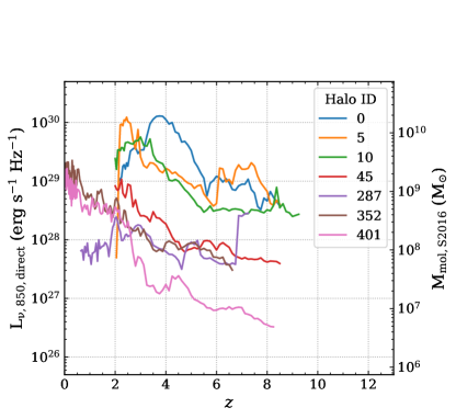
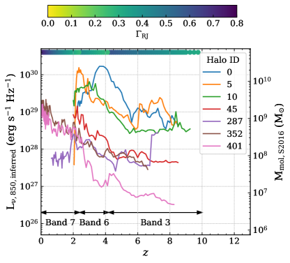
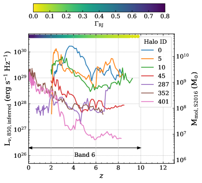
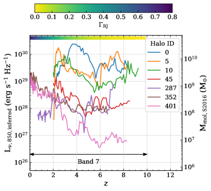
Figure 2: The monochromatic $850~{}\mu m$ luminosity, L_ν,850 as a function of redshift for the individual galaxy halos of our zoom simulations. The upper left panel shows L_{ν,850,direct}, for the ideal case where the rest-frame $850~{}\mu m$ emission can be directly observed. The upper right panel shows L_{ν,850,inferred}, where L_ν,850 is inferred from a higher rest-frequency observation. The lower row shows L_{ν,850,inferred} when only Band 6 (left) or only Band 7 observations (right) are available. In all panels aside from the upper left, the arrows mark the ranges for the ALMA band used to determine the observed frequency. The colored stripe near the top of the figure shows the $\Gamma_{\rm RJ}$ correction factor applied at a given redshift (see Appendix A of Scoville et al., 2016), assuming T${}_{\textnormal{\scriptsize{dust}}}$ $=25$ K and $\beta=1.8$. Note that the upper left panel does not require any assumptions regarding T${}_{\textnormal{\scriptsize{dust}}}$ or $\beta$. The right ordinate of all panels shows the inferred molecular gas mass using the Scoville et al. (2016) calibration with a constant $\alpha_{850}$. At high redshifts, Band 6 and 7 observations result in overestimates of of L_ν,850, of 0.5 dex (see Section 5.2).

3.2 Realistic Case: Conversion of Redshifted Observations to $850~{}\mu m$

Directly observing the rest-frame $850~{}\mu m$ observation is often not feasible, so we further emulate the common observational tactic of observing higher-frequency emission and using this to estimate S_ν,850 (and hence L_{ν,850,direct}) by assuming a dust emissivity spectral ($\beta$) index and a dust temperature (T${}_{\textnormal{\scriptsize{dust}}}$). The dust temperature enters through the Rayleigh-Jeans correction factor, $\Gamma_{\rm RJ}$ (Scoville et al., 2016). For consistency with quantities typically applied to observations we assume $\beta=1.8$ and T${}_{\textnormal{\scriptsize{dust}}}$ $=25$ K.

3.2.1 Redshift-dependent Band Selection

It is desirable to select an observing band that balances the competing requirements that this correction factor does not become too large (i.e., $\nu_{\rm rest}$ is still on the RJ tail) and where the flux density is as high as possible (to optimize integration times and detectability). Though we do not consider detection statistics and measurement noise here, we select continuum bands which would be reasonable observational choices (see e.g., Scoville et al., 2014). Specifically we use frequencies corresponding to ALMA observations at Band 7 (353 GHz) for $z\leq 2.4$, Band 6 (233 GHz) for $2.4<z<4.2$, and Band 3 (97.5 GHz) for $z\geq 4.2$ (Table 3).

Table 3: Fiducial ALMA Observing Parameters

Band	$\nu_{\rm obs}$	RMS in 1 hour
	(GHz)	(mJy beam-1)
3	097.5	0.011
6	233.0	0.013
7	343.5	0.030

Note. — These are the ALMA bands and observing frequencies assumed for deriving L_{ν,850,inferred} (Section 3.2), obtained from the ALMA Cycle 6 standard continuum frequencies. The sensitivities were obtained with the ALMA Cycle 6 sensitivity calculator and assume one hour on-source with 7.5 GHz bandwidth. Sensitivity numbers are only employed in estimating the detection prospects for the high-redshift halos (Section 6.1).

Similar to the ideal case (Section 3.1), we extract $S_{\rm\nu,obs}$ at the frequency prescribed above for the redshift of each individual snapshot. We then convert this to an estimated S_ν,850 following the procedure outlined in Scoville et al. (2016). In Figure 2 (right) we show the L_{ν,850,inferred} values inferred using this technique, for each halo as a function of $z$. Unsurprisingly, the general behavior of the inferred L_{ν,850,direct} values closely tracks that of the directly measured L_{ν,850,direct} (Figure 2, left) with the same implied range in M_mol. Encouragingly, the differences appear by eye to be relatively minor and we will assess the accuracy of the band conversion in Section 5.2.

3.2.2 Redshift-independent Band Selection

Practical considerations (i.e., availability of data) may result in observations which are not “optimal” in terms of minimizing the impact of the $\Gamma_{RJ}$ correction factor. In order to assess the recoverability of L_ν,850 under these conditions we also explore scenarios in which either ALMA Band 6 or ALMA Band 7 (Table 3) are the only observations available at all redshift. In these cases the disagreement between L_{ν,850,inferred} and L_{ν,850,direct} can be much more significant (Section 5.2).

4 Recovery of M_mol using L_ν,850

With these two “measurements” of L_ν,850 in hand, we now explore the correspondence of the implied M_mol values with the molecular gas masses of the simulations. In Figure 3 we plot the M_mol values from our simulations against L_ν,850. We also show the observed quantities used by Scoville et al. (2016) to calibrate their relationship. The M_mol values from Scoville et al. (2016) were computed from L${}^{\prime}_{\textnormal{\scriptsize{CO (1--0)}}}$ observations and $\alpha_{\rm CO}=6.5$ M_⊙ $($K km s^-1 pc${}^{2})^{-1}$. For our simulations we use the M_mol values in the snapshots, which, as a reminder, are computed in the cosmological galaxy formation simulations utilizing the Krumholz et al. (2009) model for the HI-H₂ phase balance in clouds (see Section 2).

4.1 Empirical Calibrations of $\alpha_{850}$

Scoville et al. (2016) provide two fits to their observed data: a constant $\alpha_{\nu,850}$ ($=6.7\times 10^{19}$ erg s^-1 Hz^-1 M_⊙ ^-1) and a conversion with weak L_ν,850 dependence:

$$\alpha_{\nu,850}({\rm L}_{\nu})=6.2\times 10^{19}\left(\frac{{\rm L}_{\nu}}{10^{31}{\rm~{}erg~{}s}^{-1}~{}{\rm Hz}^{-1}}\right)^{0.07}~{}{\rm erg~{}s}^{-1}~{}{\rm Hz}^{-1}~{}{\rm M}_{\odot}^{-1}$$ (3)

In Figure 3 we overplot the constant $\alpha_{\nu,850}$ as well as the luminosity-dependent $\alpha_{\nu,850}($L${}_{\nu})$.

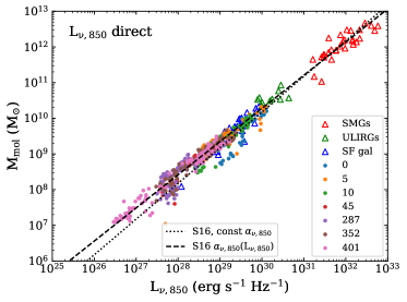
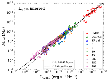
Figure 3: A comparison of the observed galaxy data and our simulations in the L_ν,850-M_mol plane. The sample used by Scoville et al. (2016), to arrive at their L_ν,850-M_mol conversion is marked with triangles. The dots mark the locations of our simulation snapshots, where L_ν,850 is obtained as described in Section 3 and M_mol is directly measured from the simulation snapshots. The dashed line corresponds to the median L_ν,850/M_mol relation of Scoville et al. (2016) while the dotted line shows their best fit. The left panel shows L_{ν,850,direct} measured directly (Section 3.1) and the right panel shows L_{ν,850,inferred} determined from higher rest-frequency observation and down-converted (Section 3.2). The molecular masses for the Scoville et al. (2016) data were obtained by them from L${}^{\prime}_{\textnormal{\scriptsize{CO (1--0)}}}$ by assuming $\alpha_{\rm CO}=6.5$ M_⊙ $($K km s^-1 pc${}^{2})^{-1}$. Note that many of the submillimeter galaxies (SMGs; red triangles) may be lensed; following Scoville et al. (2016) we are plotting their apparent luminosities here and not correcting for lensing. The luminosity-dependent calibration more closely tracks the results of our simulations.

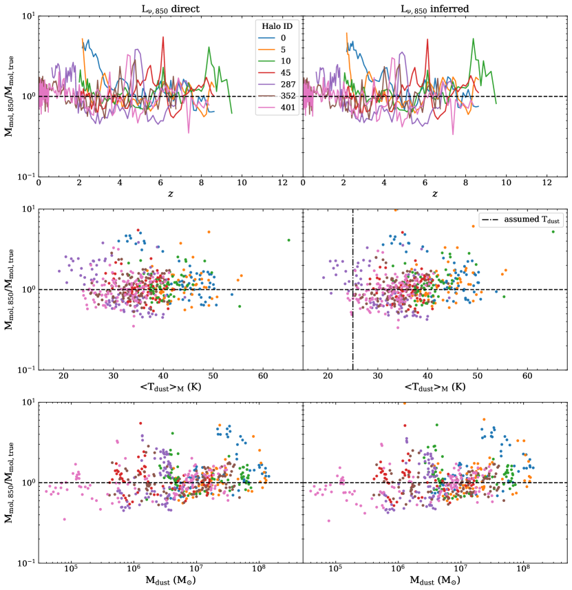
Figure 4: A comparison of M_mol values directly measured from the simulations with M_mol derived using L_ν,850 and the Scoville et al. (2016) luminosity-dependent calibration. The left column shows M_mol estimates using L_{ν,850,direct} values (Section 3.1) and the right column shows M_mol estimates using L_{ν,850,inferred} inferred from a redshifted observation (Section 3.2). In both cases, they are compared to the M_mol of the simulation snapshots (i.e., not derived from the L_ν,850 relation). From top to bottom we compare with: redshift, the mass-weighted mean T${}_{\textnormal{\scriptsize{dust}}}$, and M_dust In all panels, the horizontal black dashed line shows equality between M_mol,850 and M_mol,true. The scatter about the line of equality correlates most strongly with the galaxy-integrated gas to dust ratio. We emphasize that in obtaining M_mol from the L_{ν,850,direct} values (left column) it is not necessary to make any assumptions for T${}_{\textnormal{\scriptsize{dust}}}$ or $\beta$.

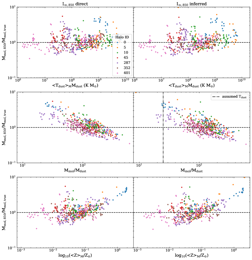
Figure 4: Continued, showing from top to bottom: the product $\langle{\rm T}_{\rm dust}\rangle_{\rm M}{\rm M}_{\rm dust}$, and the molecular gas to dust mass ratio.

In both panels of Figure 3 we find a good correlation between L_ν,850 and M_mol for our simulated galaxies. Independent of how we obtain L_ν,850 from the simulations, our snapshots more closely track the L_ν,850-dependent $\alpha_{\nu,850}$ conversion. The difference between the calibrations only exceeds a factor of two when ${\rm L}_{\nu,850}<1.5\times 10^{27}$ erg s^-1 Hz^-1. However this underestimate is systematic and should be considered when exploring samples with a range of intrinsic L_ν,850 values. We argue that the observationally calibrated L_ν,850-M_mol relation successfully recovers molecular masses for our fiducial case of a constant dust-to-metals ratio.

5 Origin of the Scatter

The relations in Figure 3 are generally tight, with a scatter of 0.2 dex about the line of equality. This scatter can be linked to contributions from physical effects (Section 5.1) and observational effects (Section 5.2). In particular it is useful to understand their origin and potential for correction to achieve a tighter relationship.

Dust heated by active galactic nuclei (AGNs) is not explicitly included in our numerical experiment, but it is worth considering whether this can add additional scatter to the L_ν,850-M_mol relation. We briefly consider the influence of this additional dust heating source in Section 5.3.

5.1 Physical Properties of the Galaxies

As noted, a L_ν,850-dependent conversion factor from L_ν,850 to M_mol seems to provide a slightly better fit for our simulated galaxies than a constant L_ν,850-M_mol relation, yet there is still scatter about the relation. In order to investigate any physical origin of the scatter, we utilize the other galaxy properties available in the simulations and summarized in Figure 1. In Figure 4 we show the ratio of the L_ν,850-inferred M_mol values (using the L_ν,850-dependent calibration) to the “true” M_mol values, against $z$, T${}_{\textnormal{\scriptsize{dust}}}$, M_dust, the product $\langle{\rm T}_{\rm dust}\rangle_{\rm M}{\rm M}_{\rm dust}$ and M_mol/M_dust.

There are no clear trends of M_mol,850/M_mol,true with redshift or T${}_{\textnormal{\scriptsize{dust}}}$. The latter is particularly interesting as it suggests that T${}_{\textnormal{\scriptsize{dust}}}$-dependent corrections will not result in more accurate estimates of M_mol from L_ν,850. Typically, the mass-weighted T${}_{\textnormal{\scriptsize{dust}}}$ is $\sim 5-15$ K higher than the $25$ K assumed when doing band conversion, but this only affects the right column of Figure 4. Based on the left column of Figure 4, which does not require any assumption about T${}_{\textnormal{\scriptsize{dust}}}$, more accurate T${}_{\textnormal{\scriptsize{dust}}}$ measurements are unlikely to lead to more accurate M_mol determinations.

In contrast, differences between M_mol,850 and M_mol,true show some correlation with M_dust. This indicates that at least some of the scatter in determining M_mol relates to variations in the dust to gas ratio. The product $\langle{\rm T}_{\rm dust}\rangle_{\rm M}{\rm M}_{\rm dust}$ (see Equation 1) shows similar correlation with M_mol,850/M_mol,true as M_dust alone does.

However, the tightest correlation is with the molecular gas to dust mass ratio (Figure 4 bottom row). It is unclear if it is possible to correct for this trend a priori, though if metallicities are available these may be used to estimate the dust to gas ratio. Encouragingly, the left and right columns of Figure 4 look similar, confirming that use of band conversion is not dominating the scatter in the relation. However, careful inspection of the figure (particularly comparing the bottom row) shows that the band conversion does slightly increase the scatter in recovery of M_mol.

5.2 The Effect of Band Conversion

The results obtained from the two techniques for determining L_ν,850 are qualitatively similar, though there are differences which arise from the band conversion. Obtaining L_{ν,850,inferred} requires assumptions for values of $\beta$ and T${}_{\textnormal{\scriptsize{dust}}}$, as well as the assumption that $\nu_{\rm rest}$ and $850~{}\mu$m lie on a single-temperature blackbody. Here we discuss the origin of the differences between L_{ν,850,direct} and L_{ν,850,inferred}, in terms of SED complexity and potential mis-match between assumed and true parameters ($\beta$, T${}_{\textnormal{\scriptsize{dust}}}$).

5.2.1 Redshift-dependent Band Selection

Here we discuss the impact of band conversion when observing bands are selected such that $\Gamma_{\rm RJ}$ is not too large.

To more clearly show the differences in L_{ν,850,direct} and L_{ν,850,inferred} for the same snapshots, in Figure 5 we show the ratio of L_{ν,850,inferred} to L_{ν,850,direct}. The inferred L_{ν,850,inferred} varies with respect to the directly measured L_{ν,850,direct}, with variations typically on the order of $10-20\%$, but up to 50%. Broadly, the variations can be separated into two categories: The first are sudden discontinuities at $z=4.2$ and $z=2.4$ which correspond to the change between ALMA bands. The jumps reflect the fact that the SEDs are not perfect single-temperature blackbodies and may arise from mismatches in the assumed T${}_{\textnormal{\scriptsize{dust}}}$ and $\beta$, so the factor of 2.3 and 1.6 change in rest frequency suddenly probes a different portion of the SED.

The remainder of the variation likely reflects mis-matches between our assumed $\beta$ and T${}_{\textnormal{\scriptsize{dust}}}$ and the true values. It is important to note that this is not the uncertainty in the use of L_ν,850 as a mass estimator but instead reflects additional uncertainty resulting from the process of inferring S_ν,850 from observations at a different rest frequency. This can readily be seen in the bottom row of Figure 4 where the scatter is visibly increased for M_mol estimates using L_{ν,850,inferred}, compared to estimates when L_{ν,850,direct} is known. We further discuss these effects in more detail in Appendix A.

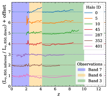
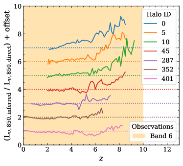
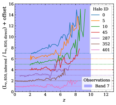
Figure 5: The ratio of the L_{ν,850,inferred} inferred using a higher rest-frequency observation and down-converting to an equivalent $850~{}\mu m$ flux (Figure 2 right) to the directly measured L_{ν,850,direct} (Figure 2 left). Clockwise from upper-left: a redshift-dependent band selection, Band 6 only, and Band 7 only. Note the difference in y-scales between the panels. For clarity the track for each halo is offset by a constant factor and the dotted lines mark the unity line for each individual halo. In the upper left panel the discontinuities at $z=4.2$ and, to a lesser degree, at $z=2.4$ originate in the change in ALMA bands (see Appendix A) and the fact that the dust SEDs are not single-temperature blackbodies. Other deviations likely reflect mismatches between the assumed parameters (T${}_{\textnormal{\scriptsize{dust}}}$, $\beta$) and their true quantities. The use of ALMA Bands 6 and 7 at $z>4-6$ results in systematic overestimation of L_ν,850, with discrepancies potentially exceeding 0.5 dex for the most massive halos.

In general the L_{ν,850,inferred} values track the directly measured L_{ν,850,direct} values when averaged over the evolution of the halo. However in this sample of galaxy formation simulations, there are systematic features in Figure 5 in certain redshift ranges for all halos. The few snapshots at $z>8$ appear to have an inferred L_{ν,850,inferred} which systematically over-estimates L_{ν,850,direct} by $>10\%$. This is likely due in part to T${}_{\textnormal{\scriptsize{dust}}}$ being $40-50$ K (Figure 1) while we assume $25$ K in the band conversion.

Figure 4 shows the mass-weighted mean T${}_{\textnormal{\scriptsize{dust}}}$ is almost always larger than the 25 K we assume; this, coupled with our fiducial study of Appendix A suggests underestimates of L_ν,850 from band conversion may result from the fact that we are sampling fluxes from a SED which is not a single-temperature blackbody. It is unlikely this can be corrected without multi-band measurements. However, this effect is small relative to the overall scatter in the L_ν,850-M_mol relation.

5.2.2 Redshift-independent Band Selection

Observing time constraints may necessitate dust continuum observations in a single band, independent of the source redshift. In Figure 5 we also show the ratio of L_{ν,850,inferred}/L_{ν,850,direct} as a function of redshift for our simulations, but assuming only Band 6 or Band 7 is used at all redshifts. At high redshifts ($z\gtrsim 5$) Bands 6 and 7 are sufficiently far from $850~{}\mu m$ that the recovery of L_ν,850 is significant compromised. For the more massive halos at $z\sim 8$, the discrepancy can exceed 0.5 dex. In these cases L_{ν,850,inferred} is systematically above L_{ν,850,direct}, and so inferences of M_mol would be biased high by the same amount (up to 0.5 dex).

5.3 The Potential Impact of AGN-heated Dust

In these simulations and post-processing we have not included radiative contributions from active galactic nuclei (AGNs). AGNs are known to have hot ($\sim 1000$ K) dust in inner 10s of parsec, owing to the intense radiation fields. Modeling of AGN tori suggests that hosts have dust warm dust masses of $10^{3}-10^{5}$ M_⊙ (Fritz et al., 2006). These dust masses are significantly smaller than the typical dust masses of our simulated galaxies (Figure 1, typically by factors $>10^{3}$. In the optically thin limit, L_ν,850 is linearly dependent on T${}_{\textnormal{\scriptsize{dust}}}$ and M_dust. Though the T${}_{\textnormal{\scriptsize{dust}}}$ of AGN-heated dust can be a factor of $\sim 30$ larger than the dust heated by star formation, the mass of dust at these high temperatures is $\sim 0.1\%$ of the total dust mass. Combining these factors, the AGN-heated dust likely has a typical contribution to L_ν,850 on the order of a few percent. This is much smaller than the scatter from physical processes (Section 5.1) and observational techniques (Section 5.2), and so is unlikely to be significant for the bulk of the galaxy population. The class of extreme highly obscured quasars may have a significant component of their far-infrared emission generated via AGN heating of dust (e.g., Wu et al., 2012; Tsai et al., 2015; Assef et al., 2015; Schneider et al., 2015; Díaz-Santos et al., 2016). Mid-infrared/submillimeter colors may be useful in identifying these objects which are likely to suffer from significant AGN contamination to the submillimeter (e.g., Stanley et al., 2017).

6 Discussion

6.1 Implications for High-$z$

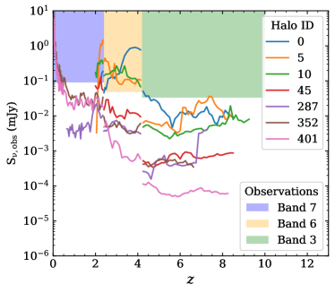
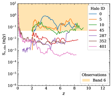
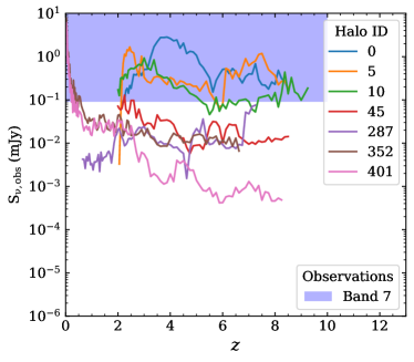
Figure 6: The observed flux density as a function of redshift for the halos in the study, for the realistic case (Section 3.2). The lower edge of the colored boxes denote the $3\sigma$ detection limit for a one hour on-source ALMA observation in the noted band (i.e., halo tracks lying inside the colored boxes would likely be detected by ALMA in our fiducial 1 hour integrations). Discontinuities in the flux curves for individual halos reflect the change in observing bands. Clockwise from upper-left: a redshift-dependent band selection, Band 6 only, and Band 7 only. The use of only Band 6 or Band 7 improves prospects for detection by taking advantage of the negative K-correction in the far infrared. However, L_{ν,850,inferred} derived from these observations are systematically high, so M_mol estimates will be similarly biased high (Section 5.2). These high-redshift detection prospects will be compromised if the dust-to-metals ratio is below the MW value (e.g., Figure 7).

We now briefly turn our attention to the approximate detectability of these systems with ALMA. In Figure 6 we show the observed flux densities as a function of redshift, for the procedure outlined in Section 3.2, mimicking typical observational approaches. The tops of the colored boxes mark the $3\sigma$ sensitivity of ALMA in one hour of on-source integration (Table 3); i.e., tracks inside the boxes are detectable, while tracks outside the boxes are not.

Over broad redshift ranges, most of our simulated galaxies are too faint to be detected in individual one hour observations. The most fertile range is around $z=3-4$ where the massive galaxies have high intrinsic dust luminosities. At higher redshifts, the more massive galaxies/halos may be individual detectable with the aid of gravitational lensing (e.g., Laporte et al., 2017).

As we note in Appendix B, the inclusion of the CMB has an important effect on the intrinsic T${}_{\textnormal{\scriptsize{dust}}}$ (and hence, monochromatic luminosities) of the galaxies at high-redshift ($z\gtrsim 6$) The absolute detectability of such high-redshift systems will also depend on their contrast against the CMB (da Cunha et al., 2013), which we do not account for in Figure 6.

6.2 Dust Formation

Large uncertainties currently exist in our understanding of the physics of dust formation. Thus it is unclear how rapidly dust masses accumulate in the early universe. Our fiducial model assumes the dust mass is a constant fraction of the metal mass. However, there is observational evidence that the dust-to-metals ratio decreases at low metallicity (Rémy-Ruyer et al., 2014), possibly connected to lower efficiencies of dust production in the ISM (Zhukovska, 2014; Popping et al., 2017) or outflows (Feldmann, 2015). This may lead to a further decrease in L_ν,850 at high-redshifts if the dust is not produced rapidly enough or if it is removed (but see Laporte et al., 2017; Strandet et al., 2017; Marrone et al., 2018, for evidence of rapid dust production by $z\approx 7-8$). This would presumably further increase the molecular gas to dust mass ratio, resulting in more significant underestimates of M_mol.

To explore the qualitative behavior we implemented a variable dust-to-metals model, following the observational results of Rémy-Ruyer et al. (2014). The details of this implementation and its effects are discussed in Appendix C. In short, we computed a metallicity-dependent dust-to-metals ratio for each gas element. This second-order effect has a noticeable impact on both the relation between L_ν,850 and M_mol and the implied detectability (Figure 7). L_ν,850 has a much steeper dependence on M_mol (i.e., on average L_ν,850 increases significantly with small increases in M_mol). Additionally, the scatter about the trend increases, reflecting the presence of a range of dust-to-metals ratios within a single halo. The net effect is that detecting continuum emission in lower-mass / lower-metallicity galaxies will be more difficult than may be expected from the Scoville et al. (2016) relation and the inferred molecular masses will be more uncertain. Comparing Figure 7 (top) with Figure 3 suggests that a variable dust-to-metals ratio implies galaxies may deviate significantly ($\gtrsim 0.5$ dex) from the Scoville et al. (2016) relation below luminosities of L_ν,850 $\lesssim 10^{28}$ ergs s^-1. However, this low-metallicity regime is similar to where simulation H₂ masses become sensitive to the adopted formation model (e.g., Popping et al., 2014; Lagos et al., 2015), meaning a more precise calibration would need to consider the effects of varying H₂ formation. In the future, models that incorporate the self-consistent formation and destruction of dust in galaxy formation simulations will be necessary to fully understand the uncertainties involved in deriving M_mol from L_{ν,850,direct} (e.g. McKinnon et al., 2016; Popping et al., 2017, Q. Li et al. in preparation).

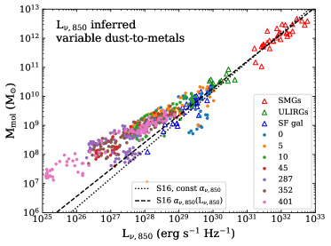
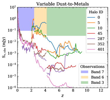
Figure 7: Top: The molecular mass in the simulation as a function of L_ν,850 for the metallicity-dependent dust-to-metals ratio (compare to Figure 3). Here the points are color-coded by the mass-weighted mean metallicity inside the 50 kpc box. Bottom: the observed flux density for the halos as a function of redshift for the same model (compare to Figure 6). This dust model predicts a L_ν,850-M_mol relation in which L_ν,850 has a steep dependence on M_mol. The scatter about the trend also increases. This is due to the variable dust-to-metals enhancing the effect of the gas within a galaxy having a range of gas metallicities. The reduced dust masses also make these galaxies more difficult to detect.

6.3 Comparison with Other Simulations

The FIRE collaboration has also explored the L_ν,850-M_mol relation using their suite of cosmological zoom simulations. Liang et al. (2018) explored this relation between $z=2-4$ for galaxies with M${}_{*}\gtrsim 10^{10}$ M_⊙. Within that redshift range, our halos 0, 5, and 10 overlap with the stellar mass range of their simulations (see Figure 1). Considering those halos within that restricted redshift range and our fiducial model for the dust-to-metals ratio, we find good agreement with their results that L_ν,850 can accurately recover M_mol and that the scatter is primarily dependent on the gas to dust ratio. This agreement is encouraging: the underlying physics driving the evolution of the Liang et al. (2018) galaxies is substantially different than those governing our own models. Beyond this, Liang et al. include the effect of obscuration by birth clouds around young stars. The general agreement between these results and our own further supports the robustness of the L_ν,850-M_mol relation for massive galaxies in this redshift range.

7 Conclusions

We present analysis of the $850~{}\mu m$ emission in simulated SEDs derived from radiative transfer post-processing of hydrodynamic cosmological zoom simulations. We find:

• L_ν,850 correlates well with M_mol in our simulations, confirming the viability of using the 850 $\mu$m emission as a molecular mass tracer for massive galaxies, independent of the assumed dust model. We find the best agreement with the M_mol values in the simulation by employing the L_ν,850-dependent calibration factor of Scoville et al. (2016). Despite the fact that the L_ν,850-dependent and constant calibrations are typically within a factor of two, the difference is systematic so we recommend the use of L_ν,850-dependent variation.

• The band conversion of redshifted flux measurements to rest-frame $850~{}\mu m$ fluxes can introduce errors typically on the order of $\sim 10-20\%$ (but sometimes up to 50%). These errors arise from mis-matches in the parameters used in the band conversion (T${}_{\textnormal{\scriptsize{dust}}}$, $\beta$) as well as from the fact that the SEDs are not single-temperature blackbodies.

• The scatter in the relation appears to be set primarily by the variations in the molecular gas to dust mass ratio. Despite a $\sim 30$ K range in T${}_{\textnormal{\scriptsize{dust}}}$ within our simulations, offsets from the mean L_ν,850-M_mol relation were not correlated with T${}_{\textnormal{\scriptsize{dust}}}$.

• Exploration of a variable dust-to-metals prescription suggests lower-metallicity / lower-mass galaxies may deviate from published L_ν,850-M_mol relations and show increased scatter about those relations. Deviations may become significant (i.e., $\gtrsim 0.5$ dex) below L_ν,850 $\lesssim 10^{28}$ erg s^-1 or $\log_{10}({\rm Z}/{\rm Z}_{\odot})\lesssim-0.8$. However, detailed dust formation models in cosmological simulations are needed to make specific predictions.

Appendix A Mismatches in Assumed T${}_{\textnormal{\scriptsize{dust}}}$ and $\beta$

Here we explore some of the effects of mis-matches between the assumed and true T${}_{\textnormal{\scriptsize{dust}}}$ and $\beta$ values. In Figure 8 we show the ratio of the inferred L_{ν,850,inferred} to the true L_{ν,850,direct} for single-temperature modified blackbodies with a range of temperatures, redshifted and “observed” following the procedure in Section 3.2 and assuming T${}_{\textnormal{\scriptsize{dust}}}$ $=25$ K and $\beta=1.8$ for the band conversion. The two panels explore mismatches in T${}_{\textnormal{\scriptsize{dust}}}$ (left) and $\beta$ (right), compared to our assumed values. In both cases, underestimating (overestimating) the value of a parameter leads to an underestimation (overestimation) of L_ν,850. This can be thought of as a manifestation of the know T–$\beta$ degeneracy in SED fitting, where a high value of one parameter can be compensated for with a lower value of the other parameter. Figure 8 clearly demonstrates that the jumps at $z=2.4$ and $z=4.2$ (corresponding to abrupt changes in the ALMA bands) reflect the impact of mis-matched T and/or $\beta$ assumptions, even in the ideal case of a single-temperature blackbody. Note that the exact locations and magnitudes of these jumps depend on the exact choice of frequencies with the ALMA bands, the redshift ranges over which each band is used to infer L_ν,850, and the degree of the mismatch in band conversion parameters (T${}_{\textnormal{\scriptsize{dust}}}$, $\beta$).

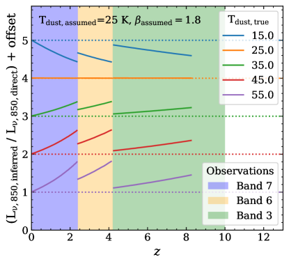
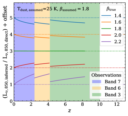
Figure 8: The application of the band conversion method of obtaining L_{ν,850,inferred} (Section 3.2) applied to ideal single-temperature blackbodies. Both panels show the ratio of L_{ν,850,inferred}/L_{ν,850,direct} as a function of redshift, employing the same ALMA band selection criterion used for the simulations in this paper. Left: We vary T${}_{\textnormal{\scriptsize{dust}}}$ of the blackbody in the range $15-55$ K (with $\beta$ fixed to 1.8) and examine the accuracy of L_{ν,850,inferred} when we assume 25 K and $\beta=1.8$ for the band conversion. Right: Holding T${}_{\textnormal{\scriptsize{dust}}}$ fixed at 25 K, we vary $\beta$ between $1.4-2.2$ and examine the accuracy of L_{ν,850,inferred} when we assume 25 K and $\beta=1.8$ for the band conversion. Underestimating T${}_{\textnormal{\scriptsize{dust}}}$ or $\beta$ results in an underestimation of L_ν,850 when performing the band conversion. For single-temperature modified blackbodies, the discrepancies can be $>50\%$ if the mis-matches are significant.

These effects are evident when using more realistic SEDs from the cosmological zoom simulations. In Figure 9 we show the ratio of inferred to true L_ν,850 for SEDs generated with powderday. Unlike in Figure 2 (right) where the intrinsic SED evolves with redshift, here we select the lowest-redshift SED for each halo and explore what L_{ν,850,inferred} would be inferred for a range of redshifts. In essence, this is a somewhat more realistic version of the test in Figure 8, using an SED which is not a single-component blackbody. The sudden jumps are still present as in Figure 8.

Mis-matches in T${}_{\textnormal{\scriptsize{dust}}}$ and $\beta$ can be up to $\sim 80\%$ (e.g., Figure 8) if the true T${}_{\textnormal{\scriptsize{dust}}}$ is $\sim 2\times$ higher than we have assumed or if $\beta$ is $\sim 20\%$ larger than we have assumed. However the single-snapshot test (Figure 9) suggests that the SEDs are typically not this pathological and that T${}_{\textnormal{\scriptsize{dust}}}$ and $\beta$ mis-matches cause errors on the order of $20\%$ if observing bands are selected on the basis of the source redshift. This is consistent with the increased scatter seen in Figure 4 (right).

In scenarios where ALMA Band 6 or 7 is used for sources at all redshifts, the discrepancy is magnified. Because T${}_{\textnormal{\scriptsize{dust}}}$ is not changing in this simplified exploration, this suggests that the use of rest frequencies far from $850~{}\mu m$ exacerbates the effect of multiple temperature components in the SEDs.

The question remains of how to determine the value of T${}_{\textnormal{\scriptsize{dust}}}$ to use when performing the band conversion. As Scoville et al. (2014) noted, SED fitting results in an estimate for the luminosity-weighted T${}_{\textnormal{\scriptsize{dust}}}$ but it is unclear how discrepant this is with the mass-weighted T${}_{\textnormal{\scriptsize{dust}}}$. In Paper II we will more closely examine the link between T${}_{\textnormal{\scriptsize{dust}}}$ values inferred from SEDs and the true underlying distribution of T${}_{\textnormal{\scriptsize{dust}}}$.

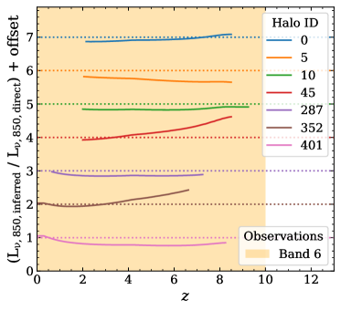
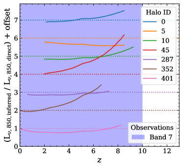
Figure 9: Here we perform an analogous study to that in Figure 8, but instead of using an ideal modified blackbody, we use an SED from the zoom simulations. We take the SED of the snapshot at $z_{\rm final}$ for each halo (Table 1, redshift it across the range probed by that halo and evaluate L_{ν,850,inferred} and L_{ν,850,direct}. This shows how the band changes affect the accuracy of L_{ν,850,inferred} determination for realistic SEDs, while removing the effects of source evolution (e.g., in T${}_{\textnormal{\scriptsize{dust}}}$). Clockwise from upper-left: a redshift-dependent band selection, Band 6 only, and Band 7 only. Comparing to the ideal blackbodies (Figure 8), L_{ν,850,inferred} is consistently underestimated for most halos when using redshift-dependent observing bands, suggesting our band conversion is overestimating T${}_{\textnormal{\scriptsize{dust}}}$ and/or $\beta$. Note that the jumps at $z=2.4$ and $z=4.4$ are still visible with a redshift-dependent band selection.

Appendix B Inclusion of the CMB

The CMB effectively imparts a temperature floor on a galaxy. Though generally negligible at low to intermediate redshifts, at high redshift the CMB approaches the rough dust temperatures of galaxies and so needs to be considered as a heating term. This heating effect has been described by da Cunha et al. (2013) for ideal blackbodies, but here we briefly discuss the effect on simulated galaxies.

Inclusion of the CMB in the radiative transfer postprocessing of the simulations has a noticeable effect on the mass-weighted mean T${}_{\textnormal{\scriptsize{dust}}}$ values for halos at $z\gtrsim 5$ (Figure 10), with increases of $10-50\%$, depending on the halo mass and redshift. This in turn translates to a higher L_ν,850 (Equation 1). Based on the agreement between the powderday L_ν,850 (including the CMB) and the simulation M_mol (Figures 3 and 4) accounting for the CMB heating is important for recovering the L_ν,850-M_mol relation for high-redshift galaxies. The increased T${}_{\textnormal{\scriptsize{dust}}}$ values only partly compensate for the building dust masses. We remind the reader that contrast effects against the CMB may complicate the measurement of L_ν,850 (da Cunha et al., 2013).

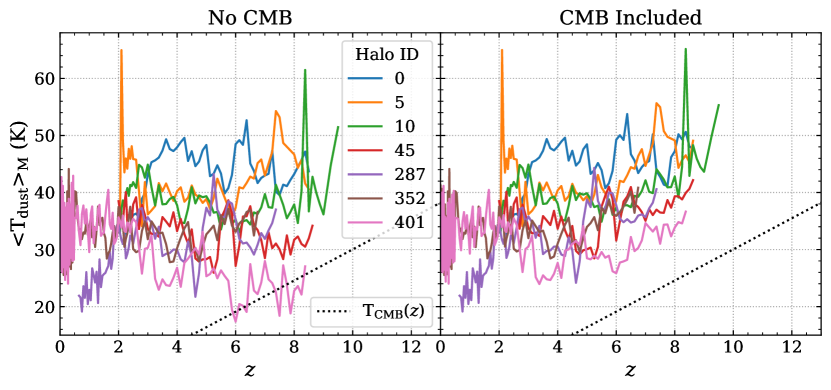
Figure 10: Comparison of the mass weighted T${}_{\textnormal{\scriptsize{dust}}}$ derived from the powderday processing without (left) and with (right) the CMB. In both panels the dotted line shows the temperature of the CMB as a function of redshift. The inclusion of the CMB affects T${}_{\textnormal{\scriptsize{dust}}}$ values for $z\gtrsim 6$, with the most pronounced differences originating in the lowest mass halos. In extreme cases, the predicted T${}_{\textnormal{\scriptsize{dust}}}$ values can fall below the CMB temperature if the CMB is not included.

Appendix C Variable Dust-to-Metals

In order to explore the impact of variable dust-to-metals ratios on L_ν,850 and $\alpha_{\nu,850}$ we implemented a metallicity-dependent dust-to-gas ratio in powderday. Rémy-Ruyer et al. (2014) parameterized this in terms of the gas-to-dust ratio as a function of $12+\log_{10}({\rm O}/{\rm H})$. We followed their fit of a single-powerlaw, using a metallicity-dependent CO to H₂ conversion factor (Table 1 of Rémy-Ruyer et al., 2014):

$$\log_{10}({\rm GDR})=2.21+2.02(8.69-12+\log_{10}({\rm O}/{\rm H}))$$ (C1)

We note that Rémy-Ruyer et al. (2014) advocate for the double powerlaw relation and this is also supported by some models (e.g., Asano et al., 2013; Zhukovska, 2014; Feldmann, 2015; Popping et al., 2017). These are cast in terms of the galaxy metallicity while our sub-grid model necessarily refers to the metallicity of individual gas particles. It is unclear how to translate between these two, so we adopt a model which does not have a discrete transition and broadly reproduces the behavior of the observations. This enables us to broadly explore the impact of variable dust-to-metals in the simulations. We expect that adopting the double powerlaw model would result in galaxies with metallicities higher than the break metallicity lying on the observed L_ν,850-M_mol relation, while those with lower metallicites would deviate from the relation. This deviation at low metallicities could be stronger for the lowest metallicity halos, owing to the steeper gas-to-dust ratio versus metallicity relation for the double powerlaw model. However, future simulations explicitly treating dust formation and destruction (Q. Li et al. in preparation) will negate the need for such coarse sub-grid prescriptions.

A variable dust-to-metals ratio is a second-order effect on the dust-to-gas ratio – decreasing metallicity reduces the dust mass in two ways: an overall reduced reservoir of metals and a smaller fraction of that reduced reservoir is in dust. We apply this prescription to individual gas elements within our snapshots, with the result that the gas in every snapshot has a range in the dust-to-metals ratio.

In Figure 11 we compare the impact of this metallicity-dependent prescription with our fiducial choice of the dust mass as a fixed fraction of the metal mass. The effect is most pronounced at high redshift and low metallicity, where the metallicity-dependent gas-to-dust ratio (GDR) results in lower metal masses and higher mass-weighted dust temperatures, compared to the fiducial simulations with constant dust-to-metals ratios.

The details of the dust mass growth also change when adopting this prescription. Accretion of low-metallicity gas brings in significantly less dust due to this second-order effect. Relative to the fixed dust-to-metals model, the dust temperatures increase by up to $\sim 50\%$ and the dust masses may drop by up two dex. In sum, L_ν,850 typically decreases when considering a variable dust-to-metals situation.

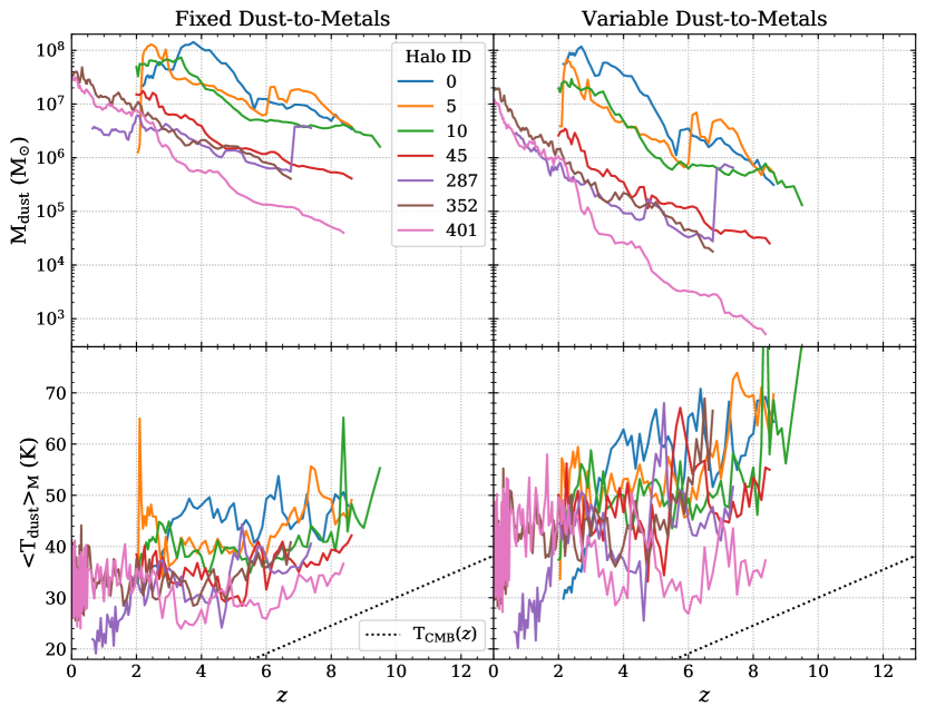
Figure 11: The impact of the Rémy-Ruyer et al. (2014) dust prescription on the inferred dust masses and temperatures in the zoom simulations. Left: the fiducial case where the dust is a fixed fraction of the metal mass (identical to Figure 1). Right: a metallicity-dependent gas-to-dust ratio following the Rémy-Ruyer et al. (2014) prescription described in the text. The metallicity-dependent gas-to-dust ratio shows significantly lower dust masses at low metallicity / high redshift and higher dust temperatures. The shape of the M_dust evolution curves also changes in detail, likely a result of accretion or merger events bringing in preferentially metal-poor gas, where the reduced dust mass is further amplified by the variable dust-to-metals prescription.

C.1 Impact on H₂ Formation

Efficient H₂ formation relies on dust as a catalyst (e.g., Gould & Salpeter, 1963), so in addition to the reduction in dust mass, a variable dust-to-metals ratio should also affect the formation of H₂. This results in an inconsistency in our treatment of the variable dust-to-metals as a reduced H₂ formation efficiency may bring the snapshots in Figure 7 back towards the empirical relation found for metal-rich galaxies. The increased dust temperatures resulting from a reduced dust mass may also affect the H₂ formation (e.g., Cazaux & Spaans, 2004). Assessing the magnitude of this effect would require a new suite of cosmological zoom simulations modifying the H₂ formation model to explicitly consider the dust mass (rather than using the metallicity and assuming a constant dust-to-metals ratio) and is beyond the scope of this paper. Future work with explicit treatment of dust formation and destruction (Q. Li et al. in preparation) will be able to specifically address this inconsistency in our treatment.

However we emphasize that the low mass / low metallicity halos are the ones affected by this inconsistency. Their lowered dust masses in the variable dust-to-metals scenario make them, at best, challenging to detect with current facilities.

Appendix D Sub-resolution Birth Clouds

Dust reprocessing of the UV/optical radiation field can occur on the scales of the individual clouds in which star clusters form. These “birth clouds” are below the resolution limit of our simulations, so including them requires the addition of a sub-grid model for the radiative transfer and time evolution. To explore the impact of including birth clouds, we re-ran the radiative transfer for halo 401, using the Charlot & Fall (2000) model as implemented in fsps (Conroy et al., 2009) with the default values.

In Figure 12 we reproduce Figure 3 for the halo 401 snapshots with the birth cloud model enabled. The inclusion of the birth cloud model still shows a relatively tight sequence, however it is offset to higher L_ν,850 by 1–2 dex. This is likely due to compact dust in/around star forming regions resulting in a larger optical depth to IR photons and producing an overall cooler SED with significantly more emission at long wavelengths. This appears inconsistent with the observations as it predicts an excess of L_ν,850 over what is observed.

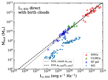
Figure 12: The same as Figure 3 but showing only halo 401 with the default birth cloud model of Charlot & Fall (2000) as implemented in Conroy et al. (2009). The L_ν,850 is significantly over-predicted at fixed M_mol, compared to the observed galaxies presented in Scoville et al. (2016).

As implemented in fsps+powderday the birth cloud model likely produces too much opacity, as the dust within the birth clouds is not consistently modeled with the rest of the ISM in the hydrodynamic simulation. This birth cloud model thus effectively means the ISM is too dust rich. It may be possible to adjust the parameters of the birth cloud model to reduce the L_ν,850 excess. However, the parameters for the birth clouds are largely unknown. The default values from Charlot & Fall (2000) were chosen to be consistent with galaxy-integrated observational properties of starbursts and as such may not be precise enough for the treatment of individual clouds in a sub-grid model. There is ongoing debate regarding the timescale on which gas is cleared from the clusters (see e.g., Prescott et al., 2007; Whitmore et al., 2014; Calzetti et al., 2015; Johnson et al., 2015; Murphy et al., 2018) Furthermore, this clearing timescale may be a function of the star cluster environment.

However, the fact that our simulations (Figure 3; without the birth cloud model) are consistent with the observations, this suggests that the radiative transfer effects and dust heating dominating the L_ν,850 emission of galaxies may occur on the scales which are robustly probed by our simulations (i.e., $\gtrsim 10-50$ pc).

References

- Abruzzo et al. (2018) Abruzzo, M. W., Narayanan, D., Davé, R., & Thompson, R. 2018, ArXiv e-prints, arXiv:1803.02374
- Asano et al. (2013) Asano, R. S., Takeuchi, T. T., Hirashita, H., & Nozawa, T. 2013, MNRAS, 432, 637
- Assef et al. (2015) Assef, R. J., Eisenhardt, P. R. M., Stern, D., et al. 2015, ApJ, 804, doi:10.1088/0004-637X/804/1/27
- Bertemes et al. (2018) Bertemes, C., Wuyts, S., Lutz, D., et al. 2018, ArXiv e-prints, arXiv:1803.08926
- Blitz & Rosolowsky (2006) Blitz, L., & Rosolowsky, E. 2006, ApJ, 650, 933
- Bolatto et al. (2013) Bolatto, A. D., Wolfire, M., & Leroy, A. K. 2013, ARA&A, 51, 207
- Bruzual & Charlot (2003) Bruzual, G., & Charlot, S. 2003, MNRAS, 344, 1000
- Calzetti et al. (2015) Calzetti, D., Johnson, K. E., Adamo, A., et al. 2015, ApJ, 811, 75
- Casey et al. (2014) Casey, C. M., Narayanan, D., & Cooray, A. 2014, Physics Reports, 541, 45
- Cazaux & Spaans (2004) Cazaux, S., & Spaans, M. 2004, ApJ, 611, 40
- Chabrier (2003) Chabrier, G. 2003, PASP, 115, 763
- Charlot & Fall (2000) Charlot, S., & Fall, S. M. 2000, ApJ, 539, 718
- Conroy & Gunn (2010) Conroy, C., & Gunn, J. E. 2010, ApJ, 712, 833
- Conroy et al. (2009) Conroy, C., Gunn, J. E., & White, M. 2009, ApJ, 699, 486
- Conroy et al. (2010) Conroy, C., White, M., & Gunn, J. E. 2010, ApJ, 708, 58
- da Cunha et al. (2013) da Cunha, E., Groves, B., Walter, F., et al. 2013, ApJ, 766, 13
- Davé et al. (2011) Davé, R., Finlator, K., & Oppenheimer, B. D. 2011, arXiv/1108.0426, arXiv:1108.0426
- Davé et al. (2017a) Davé, R., Rafieferantsoa, M. H., & Thompson, R. J. 2017a, arXiv/1704.01335, arXiv:1704.01135
- Davé et al. (2017b) Davé, R., Rafieferantsoa, M. H., Thompson, R. J., & Hopkins, P. F. 2017b, MNRAS, arXiv:1610.01626
- Davé et al. (2016) Davé, R., Thompson, R., & Hopkins, P. F. 2016, MNRAS, 462, 3265
- Díaz-Santos et al. (2016) Díaz-Santos, T., Assef, R. J., Blain, A. W., et al. 2016, ApJ, 816, doi:10.3847/2041-8205/816/1/L6
- Draine (2003) Draine, B. T. 2003, ARA&A, 41, 241
- Draine & Li (2007) Draine, B. T., & Li, A. 2007, ApJ, 657, 810
- Dwek (1998) Dwek, E. 1998, ApJ, 501, 643
- Feldmann (2015) Feldmann, R. 2015, MNRAS, 449, 3274
- Fritz et al. (2006) Fritz, J., Franceschini, A., & Hatziminaoglou, E. 2006, MNRAS, 366, 767
- Gnedin & Draine (2014) Gnedin, N. Y., & Draine, B. T. 2014, ApJ, 795, 37
- Gnedin & Kravtsov (2011) Gnedin, N. Y., & Kravtsov, A. V. 2011, ApJ, 728, 88
- Gould & Salpeter (1963) Gould, R. J., & Salpeter, E. E. 1963, ApJ, 138, 393
- Groves et al. (2004) Groves, B. A., Dopita, M. A., & Sutherland, R. S. 2004, ApJS, 153, 9
- Groves et al. (2015) Groves, B. A., Schinnerer, E., Leroy, A., et al. 2015, ApJ, 799, 96
- Hahn & Abel (2011) Hahn, O., & Abel, T. 2011, MNRAS, 415, 2101
- Hopkins (2015) Hopkins, P. F. 2015, MNRAS, 450, 53
- Hopkins (2017) —. 2017, arXiv/1712.01294, arXiv:1712.01294
- Hopkins et al. (2014) Hopkins, P. F., Kereš, D., Oñorbe, J., et al. 2014, MNRAS, 445, 581
- Hopkins et al. (2013) Hopkins, P. F., Narayanan, D., Murray, N., & Quataert, E. 2013, MNRAS, 433, 69
- Hopkins et al. (2017) Hopkins, P. F., Wetzel, A., Keres, D., et al. 2017, arXiv/1702.06148, arXiv:1702.06148
- Hughes et al. (2017) Hughes, T. M., Ibar, E., Villanueva, V., et al. 2017, MNRAS, 468, L103
- Hunter (2007) Hunter, J. D. 2007, Computing In Science & Engineering, 9, 90
- Iwamoto et al. (1999) Iwamoto, K., Brachwitz, F., Nomoto, K., et al. 1999, ApJS, 125, 439
- Janowiecki et al. (2018) Janowiecki, S., Cortese, L., Catinella, B., & Goodwin, A. J. 2018, MNRAS, 476, 1390
- Johnson et al. (2015) Johnson, K. E., Leroy, A. K., Indebetouw, R., et al. 2015, ApJ, 806, 35
- Jonsson et al. (2010) Jonsson, P., Groves, B. A., & Cox, T. J. 2010, MNRAS, 186
- Kennicutt & Evans (2012) Kennicutt, R. C., & Evans, N. J. 2012, ARA&A, 50, 531
- Kennicutt (1998) Kennicutt, Jr., R. C. 1998, ApJ, 498, 541
- Kroupa (2002) Kroupa, P. 2002, Science, 295, 82
- Krumholz (2013) Krumholz, M. R. 2013, MNRAS, 436, 2747
- Krumholz et al. (2009) Krumholz, M. R., McKee, C. F., & Tumlinson, J. 2009, ApJ, 693, 216
- Lagos et al. (2015) Lagos, C. d. P., Crain, R. A., Schaye, J., et al. 2015, MNRAS, 452, 3815
- Laporte et al. (2017) Laporte, N., Ellis, R. S., Boone, F., et al. 2017, ApJ, 837, L21
- Liang et al. (2018) Liang, L., Feldmann, R., Faucher-Giguère, C.-A., et al. 2018, arXiv/1804.02403, arXiv:1804.02403
- Lucy (1999) Lucy, L. B. 1999, A&A, 344, 282
- Magdis et al. (2012) Magdis, G. E., Daddi, E., Béthermin, M., et al. 2012, ApJ, 760, 6
- Marigo & Girardi (2007) Marigo, P., & Girardi, L. 2007, A&A, 469, 239
- Marigo et al. (2008) Marigo, P., Girardi, L., Bressan, A., et al. 2008, A&A, 482, 883
- Marrone et al. (2018) Marrone, D. P., Spilker, J. S., Hayward, C. C., et al. 2018, Nature, 553, 51
- McKinnon et al. (2016) McKinnon, R., Torrey, P., & Vogelsberger, M. 2016, MNRAS, 457, 3775
- Muratov et al. (2015) Muratov, A. L., Kereš, D., Faucher-Giguère, C.-A., et al. 2015, MNRAS, 454, 2691
- Murphy et al. (2018) Murphy, E. J., Dong, D., Momjian, E., et al. 2018, ApJS, 234, 24
- Narayanan et al. (2018a) Narayanan, D., Conroy, C., Dave, R., Johnson, B., & Popping, G. 2018a, ArXiv e-prints, arXiv:1805.06905
- Narayanan et al. (2008) Narayanan, D., Cox, T. J., Shirley, Y., et al. 2008, ApJ, 684, 996
- Narayanan et al. (2018b) Narayanan, D., Davé, R., Johnson, B. D., et al. 2018b, MNRAS, 474, 1718
- Narayanan et al. (2010) Narayanan, D., Hayward, C. C., Cox, T. J., et al. 2010, MNRAS, 401, 1613
- Narayanan et al. (2012) Narayanan, D., Krumholz, M. R., Ostriker, E. C., & Hernquist, L. 2012, MNRAS, 421, 3127
- Narayanan et al. (2015) Narayanan, D., Turk, M., Feldmann, R., et al. 2015, Nature, 525, 496
- Nomoto et al. (2006) Nomoto, K., Tominaga, N., Umeda, H., Kobayashi, C., & Maeda, K. 2006, Nuclear Physics A, 777, 424
- Olsen et al. (2017) Olsen, K., Greve, T. R., Narayanan, D., et al. 2017, ApJ, 846, 105
- Oppenheimer & Davé (2008) Oppenheimer, B. D., & Davé, R. 2008, MNRAS, 387, 577
- Pérez & Granger (2007) Pérez, F., & Granger, B. E. 2007, Computing in Science and Engineering, 9, 21
- Planck Collaboration et al. (2014) Planck Collaboration, Ade, P. A. R., Aghanim, N., et al. 2014, A&A, 571, A16
- Popping et al. (2017) Popping, G., Somerville, R. S., & Galametz, M. 2017, MNRAS, 471, 3152
- Popping et al. (2014) Popping, G., Somerville, R. S., & Trager, S. C. 2014, MNRAS, 442, 2398
- Prescott et al. (2007) Prescott, M. K. M., Kennicutt, Jr., R. C., Bendo, G. J., et al. 2007, ApJ, 668, 182
- Rémy-Ruyer et al. (2014) Rémy-Ruyer, A., Madden, S. C., Galliano, F., et al. 2014, A&A, 563, A31
- Robitaille (2011) Robitaille, T. P. 2011, A&A, 536, A79
- Robitaille et al. (2012) Robitaille, T. P., Churchwell, E., Benjamin, R. A., et al. 2012, A&A, 545, A39
- Sandstrom et al. (2013) Sandstrom, K. M., Leroy, A. K., Walter, F., et al. 2013, ApJ, 777, 5
- Schaye et al. (2015) Schaye, J., Crain, R. A., Bower, R. G., et al. 2015, MNRAS, 446, 521
- Schinnerer et al. (2016) Schinnerer, E., Groves, B., Sargent, M. T., et al. 2016, ApJ, 833, 112
- Schmidt (1959) Schmidt, M. 1959, ApJ, 129, 243
- Schneider et al. (2015) Schneider, R., Bianchi, S., Valiante, R., Risaliti, G., & Salvadori, S. 2015, A&A, 579, doi:10.1051/0004-6361/201526105
- Scoville et al. (2014) Scoville, N., Aussel, H., Sheth, K., et al. 2014, ApJ, 783, 84
- Scoville et al. (2016) Scoville, N., Sheth, K., Aussel, H., et al. 2016, ApJ, 820, 83
- Scoville et al. (2017) Scoville, N., Lee, N., Vanden Bout, P., et al. 2017, ApJ, 837, 150
- Stanley et al. (2017) Stanley, F., Harrison, C. M., Alexander, D. M., et al. 2017, ArXiv e-prints, arXiv:1712.02363
- Strandet et al. (2017) Strandet, M. L., Weiss, A., De Breuck, C., et al. 2017, ApJ, 842, L15
- The Astropy Collaboration et al. (2013) The Astropy Collaboration, Robitaille, T. P., Tollerud, E. J., et al. 2013, A&A, 558, A33
- The Astropy Collaboration et al. (2018) The Astropy Collaboration, Price-Whelan, A. M., Sipőcz, B. M., et al. 2018, ArXiv e-prints, arXiv:1801.02634
- Thompson et al. (2014) Thompson, R., Nagamine, K., Jaacks, J., & Choi, J.-H. 2014, ApJ, 780, 145
- Tsai et al. (2015) Tsai, C.-W., Eisenhardt, P. R. M., Wu, J., et al. 2015, ApJ, 805, doi:10.1088/0004-637X/805/2/90
- Turk et al. (2011) Turk, M. J., Smith, B. D., Oishi, J. S., et al. 2011, ApJS, 192, 9
- Van Der Walt et al. (2011) Van Der Walt, S., Colbert, S. C., & Varoquaux, G. 2011, ArXiv e-prints, arXiv:1102.1523
- Vladilo (1998) Vladilo, G. 1998, ApJ, 493, 583
- Watson (2011) Watson, D. 2011, A&A, 533, A16
- Weingartner & Draine (2001) Weingartner, J. C., & Draine, B. T. 2001, ApJ, 548, 296
- Whitmore et al. (2014) Whitmore, B. C., Brogan, C., Chandar, R., et al. 2014, ApJ, 795, 156
- Wu et al. (2012) Wu, J., Tsai, C.-W., Sayers, J., et al. 2012, ApJ, 756, doi:10.1088/0004-637X/756/1/96
- Zhukovska (2014) Zhukovska, S. 2014, A&A, 562, A76