Abstract

Motivated by recent experimental measurements on flavour physics, in tension with Standard Model predictions, we perform an updated analysis of New Physics violating Lepton Flavour Universality, by using the effective Lagrangian approach and in the $Z^{{}^{\prime}}$ and $S_{3}$ leptoquark models. We explicitly analyze the impact of considering complex Wilson coefficients in the analysis of $B$-anomalies, by performing a global fit of $R_{K}$ and $R_{K^{*0}}$ observables, together with $\Delta M_{s}$ and $A_{CP}^{\rm{mix}}$. The inclusion of complex couplings provides a slightly improved global fit, and a marginally improved $\Delta M_{s}$ prediction.

1 Introduction

At present, many interesting measurements on flavour physics are performed at the LHC [1, 2, 3, 5, 4, 6, 7, 8, 9, 10, 11, 12, 13, 14]. Some relevant flavour transition processes in order to constrain new physics at the LHC are the leptonic, semi-leptonic, baryonic and radiative exclusive decays. Some of these decays allow us to build optimized observables, as ratios of these decays, that are theoretically clean observables and whose measurements are in tension with Standard Model (SM) predictions. One example is the case of observables in $b\rightarrow sll$ transitions. Recently, the LHCb collaboration observed a deviation from the SM predictions in the neutral-current $b\rightarrow s$ transition [1, 2, 5, 6, 7, 11, 13], hinting at lepton flavour universality violation effects. The results for ratios of branching ratios involving different lepton flavours are given by [2, 11, 13],

$${R_{K}=\frac{{\cal B}(B^{+}\to K^{+}\mu^{+}\mu^{-})}{{\cal B}(B^{+}\to K^{+}e^{+}e^{-})}} = 0.745^{+0.090}_{-0.074}\pm 0.0036\,\,\,\,1\,{\rm GeV}^{2}<q^{2}<6\,{\rm GeV}^{2}$$

$${R_{K^{*0}}=\frac{{\cal B}(B^{0}\to K^{*0}\mu^{+}\mu^{-})}{{\cal B}(B^{0}\to K^{*0}e^{+}e^{-})}} = 0.660^{+0.110}_{-0.070}\pm 0.024\,\,\,\,\,\,\,0.045\,{\rm GeV}^{2}<q^{2}<1.1\,{\rm GeV}^{2}$$ (1)

$$0.685^{+0.113}_{-0.069}\pm 0.047\,\,\,\,\,\,1.1\,{\rm GeV}^{2}<q^{2}<6\,{\rm GeV}^{2}$$

where the first uncertainty is statistical and the second one comes from systematic effects. In the SM $R_{K}=R_{K^{*0}}=1$ with theoretical uncertainties of the order of $1\%$ [15, 16], as a consequence of Lepton Flavour Universality. The compatibility of the above results with respect to the SM predictions is of $2.6\,\sigma$ deviation in the first case and for $R_{K^{*0}}$, in the low $q^{2}$ di-lepton invariant mass region is of about $2.3$ standard deviations; being in the central$-q^{2}$ of $2.4\,\sigma$. A discrepancy of about $3\,\sigma$ is found when the measurements of $R_{K}$ and $R_{K^{*0}}$ are combined [17]. Anomalous deviations were also observed in the angular distributions of the decay rate of $B\to K^{*}\mu^{+}\mu^{-}$, being the most significant discrepancy for the $P_{5}^{{}^{\prime}}$ observable [1, 6]. The Belle Collaboration has also reported a discrepancy in angular observables consistent with LHCb results [18]. In addition, ATLAS and CMS collaborations have presented their updated results for the angular parameters of the $B$ meson decay, $B^{0}\to K^{0}\mu^{+}\mu^{-}$ [19, 20, 21, 22].

A great theoretical effort has been devoted to the understanding of these deviations, see for example [15, 17, 23, 24, 25, 26, 27, 28, 29, 30, 31, 32, 33, 34, 35, 36, 37, 38, 39, 40, 41, 42] and references therein. From the theoretical side, the ratios $R_{K}$ and $R_{K^{*0}}$ are very clean observables; essentially free of hadronic uncertainties that cancel in the ratios [15]. The experimental data has been used to constrain New Physics (NP) models. One useful way to analyze the effects of NP in these observables and to quantify the possible deviations from the SM predictions is through the effective Hamiltonian approach, allowing us a model-independent analysis of new physics effects. In addition, one can compute this effective Hamiltonian in the context of specific NP models. It has been shown that $Z^{{}^{\prime}}$ and leptoquark models could explain the $R_{K},R_{K^{*0}}$ deviations.

On the other hand, NP models are also severely constrained by other flavour observables, for example in $B_{s}-$mixing. Recently an updated computation for the $B_{s}$ mesons mass difference in the SM has been presented [43, 44, 45, 46, 47], which shows a deviation with the experimental result [47, 48]:

$$\Delta M_{s}^{\rm{exp}}=(17.757\pm 0.021)\,{\rm ps}^{-1}\,,\,\,\,\,{\Delta M_{s}^{\rm{SM}}}=(20.01\pm 1.25)\,{\rm ps}^{-1}\,,$$ (2)

such that ${\Delta M_{s}^{\rm{SM}}}>\Delta M_{s}^{\rm{exp}}$ at about $2\,\sigma$. This fact imposes additional constraints over the NP parameter space. Therefore, a global fit is mandatory when considering all updated flavour observables. A negative contribution to $\Delta M_{s}$ is needed to reconcile it with the experimental result, in the context of some NP models (like $Z^{{}^{\prime}}$ or leptoquarks) it implies complex Wilson coefficients in the effective Hamiltonian of $R_{K},R_{K^{*0}}$ [47] (see also below). To the best of our knowledge, most previous works have used only real Wilson coefficients in global fits of $R_{K}$ and $R_{K^{*0}}$ observables together with $\Delta M_{s}$, an exception being Ref.[34]. An effect of introducing complex couplings is the generation of $CP$ asymmetries. The mixing-induced $CP$ asymmetry in the $B$-sector can be measured through $A_{CP}^{\rm{mix}}\equiv A_{CP}^{\rm{mix}}(B_{s}\to J/\psi\phi)\equiv\sin(\phi_{s}^{c\bar{c}s})$, experimentally it is measured to be [48]:

$$A_{CP}^{\rm{mix}}{}^{\rm\ exp}(B_{s}\to J/\psi\phi)=-0.021\pm 0.031\ \ .$$ (3)

In the SM it is given by $A_{CP}^{\rm{mix}}{}^{\rm\ SM}=\sin(-2\beta_{s})$[47, 49, 50], with $\beta_{s}=0.01852\pm 0.00032$[51] we obtain $A_{CP}^{\rm{mix}}{}^{\rm\ SM}=-0.03703\pm 0.00064$, which is consistent with the experimental result (3) at the $\sim 0.5\,\sigma$ level.

Ref.[34] performed fits for the $B$-decay physics observables using complex Wilson coefficients, in the model independent and model dependent approaches. The analysis of Ref.[34] performs fits for the $B$-decay observables using complex couplings, without including the $\Delta M_{s}$ or $A_{CP}^{\rm{mix}}$ observables, then Ref.[34] proceeds to provide predictions to $CP$-violation observables. Ref.[34] only includes $\Delta M_{s}$ and $A_{CP}^{\rm{mix}}$ in the $Z^{\prime}$-model fit. Our results agree with the ones of Ref.[34] wherever comparable.

The aim of the present work is to investigate the effects of complex Wilson coefficients in the global analyses of NP in $B$-meson anomalies. We assume a model independent effective Hamiltonian approach and we study the region of NP parameter space compatible with the experimental data, by considering the dependence of the results on the assumptions of imaginary and/or complex Wilson coefficients. We compare our results with the case of considering only real Wilson coefficients. A brief summary of the NP contributions to the effective Lagrangian relevant for $b\to s\ell\ell$ transitions and $B_{s}$-mixing is presented in Section 2, where we also recall the need to consider complex Wilson coefficients in the analysis. In Section 3 we discuss the effects of having imaginary or complex Wilson coefficients on $R_{K}$ observables. The impact of these complex Wilson coefficients in the analysis of $B$-meson anomalies in two specific models, $Z^{{}^{\prime}}$ and leptoquarks, is included in Section 4. We consider a global fit of $R_{K}$ and $R_{K^{*0}}$ observables, together with $\Delta M_{s}$ and $CP$-violation observable $A_{CP}^{\rm{mix}}$ in this analysis. Finally, conclusions are given in Section 5.

2 Effective Hamiltonians and new physics models

The effective Lagrangian for $b\to s\ell\ell$ transitions is conventionally given by [52],

$$\mathcal{L}_{\text{eff}}=-\frac{4\,G_{F}}{\sqrt{2}}V_{tb}V_{ts}^{*}\sum_{i,\ell}(C_{i}^{\ell}O_{i}^{\ell}+C_{i}^{\prime\,\ell}O_{i}^{\prime\,\ell})+\text{h.c.}\,,$$ (4)

being $O_{i}^{(\prime)\,\ell}$ $(\ell=e,\mu)$ the operators and $C_{i}^{(\prime)\,\ell}$ the corresponding Wilson coefficients. The relevant semi-leptonic operators for explaining deviation in $R_{K}$ observables, eq. (1), can be defined as,

$$O_{9}^{\ell} =\frac{e^{2}}{16\pi^{2}}(\bar{s}\gamma_{\mu}P_{L}b)(\bar{\ell}\gamma^{\mu}\ell)\,, \!\!\!\!\!O_{9}^{\prime\,\ell} =\frac{e^{2}}{16\pi^{2}}(\bar{s}\gamma_{\mu}P_{R}b)(\bar{\ell}\gamma^{\mu}\ell)\,,$$ (5)

$$O_{10}^{\ell} =\frac{e^{2}}{16\pi^{2}}(\bar{s}\gamma_{\mu}P_{L}b)(\bar{\ell}\gamma^{\mu}\gamma_{5}\ell)\,, \!\!\!\!\!O_{10}^{\prime\,\ell} =\frac{e^{2}}{16\pi^{2}}(\bar{s}\gamma_{\mu}P_{R}b)(\bar{\ell}\gamma^{\mu}\gamma_{5}\ell)\,.$$ (6)

The Wilson coefficients have contributions from the SM and NP,

$$C_{i}^{(\prime)\,\ell}=C_{i}^{(\prime)\,\mathrm{SM}\,\ell}+C_{i}^{(\prime)\,\mathrm{NP}\,\ell}\ \ .$$

In the present work we analyze the NP contributions $C_{i}^{(\prime)\,\mathrm{NP}\,\ell}$. In most of our analysis we will consider the left-handed Wilson coefficients $C_{i}^{\mathrm{NP}\,\ell}$, the righ-handed Wilson coefficients $C_{i}^{\prime\,\mathrm{NP}\,\ell}$ are treated briefly in the model-independent approach of Section 3 (see Table 1 below). The NP contributions to $B_{s}$-mixing are described by the effective Lagrangian [52]:

$$\mathcal{L}^{\rm{NP}}_{\Delta B=2}=-\frac{4G_{F}}{\sqrt{2}}\left(V_{tb}V^{*}_{ts}\right)^{2}\left[C_{bs}^{LL}\left(\bar{s}_{L}\gamma_{\mu}b_{L}\right)^{2}+\text{h.c.}\right]\,,$$ (7)

where $C_{bs}^{LL}$ is a Wilson coefficient. In order to study the allowed NP parameter space we follow the same procedure as given in [47], comparing the experimental measurement of the mass difference with the prediction in the SM and NP. Therefore, the effects can be parametrized as [47],

$$\frac{\Delta M_{s}}{\Delta M_{s}^{\rm{SM}}}=\left|1+\frac{C_{bs}^{LL}}{R^{\rm{loop}}_{\rm{SM}}}\right|\,,$$ (8)

where $R^{\rm loop}_{\rm SM}=1.3397\times 10^{-3}$ [47]. The NP prediction to the $CP$-asymmetry $A_{CP}^{\rm{mix}}$ is given by[47, 49, 50]

$$A_{CP}^{\rm{mix}}=\sin(\phi_{\Delta}-2\beta_{s})\ \ \ ,\ \ \ \phi_{\Delta}={\rm Arg}\left(1+\frac{C_{bs}^{LL}}{R^{\rm{loop}}_{\rm{SM}}}\right)\ \ \ ,$$ (9)

where $\beta_{s}$ and $R^{\rm loop}_{\rm SM}$ have been given above.

Since $\Delta M_{s}^{\rm{exp}}<{\Delta M_{s}^{\rm{SM}}}$ (2), eq. (8) tells us that to obtain a prediction of $\Delta M_{s}$ closer to $\Delta M_{s}^{\rm{exp}}$ the NP Wilson coefficient $C_{bs}^{LL}$ (7) must be negative ($C_{bs}^{LL}<0$). In a generic effective Hamiltonian approach, each Wilson coefficient is independent, and setting $C_{bs}^{LL}<0$ has no effect on $C_{9}^{\rm{NP}\,\mu}$, $C_{10}^{\rm{NP}\,\mu}$, etc. However, explicit NP models give predictions on the Wilson coefficients which introduce correlations among them. We will concentrate on two specific models that have been proposed to solve the semi-leptonic $B_{s}$-decay anomalies: $Z^{\prime}$ and leptoquarks.

We start with the $Z^{{}^{\prime}}$ model that contains a $Z^{{}^{\prime}}$ boson with mass $M_{Z^{{}^{\prime}}}$ and whose extra NP operators can involve different chiralities. The part of the effective Lagrangian relevant for $b\to s\mu^{+}\mu^{-}$ transitions and $B_{s}$-mixing is given by [47],

$$\mathcal{L}_{Z^{\prime}}^{\rm eff} = -\frac{1}{2M^{2}_{Z^{\prime}}}\left(\lambda^{Q}_{ij}\,\bar{d}_{L}^{i}\gamma_{\mu}d_{L}^{j}+\lambda^{L}_{\alpha\beta}\,\bar{\ell}_{L}^{\alpha}\gamma_{\mu}\ell_{L}^{\beta}\right)^{2}$$

$$\sim -\frac{1}{2M^{2}_{Z^{\prime}}}\left[(\lambda^{Q}_{23})^{2}\left(\bar{s}_{L}\gamma_{\mu}b_{L}\right)^{2}+2\lambda^{Q}_{23}\lambda^{L}_{22}(\bar{s}_{L}\gamma_{\mu}b_{L})(\bar{\mu}_{L}\gamma^{\mu}\mu_{L})+\text{h.c.}\right]+\cdots\,,$$

where $d^{i}$ and $\ell^{\alpha}$ denote down-quark and charged-lepton mass eigenstates, and $\lambda^{Q}$ and $\lambda^{L}$ are hermitian matrices in flavour space. When matching the above equation with eqs. (4) and (7) one obtains the expressions for the Wilson coefficients at the tree level [47],

$$C_{9}^{\rm{NP}\,\mu}=-C_{10}^{\rm{NP}\,\mu}=-\frac{\pi}{\sqrt{2}G_{F}M^{2}_{Z^{\prime}}\alpha}\left(\frac{\lambda^{Q}_{23}\lambda^{L}_{22}}{V_{tb}V^{*}_{ts}}\right)\,,$$ (11)

and

$$C_{bs}^{LL}=\frac{\eta^{LL}(M_{Z^{\prime}})}{4\sqrt{2}G_{F}M^{2}_{Z^{\prime}}}\left(\frac{\lambda^{Q}_{23}}{V_{tb}V^{*}_{ts}}\right)^{2}\,,$$ (12)

where $\eta^{LL}(M_{Z^{\prime}})>0$ encodes the running down to the bottom mass scale.

From (12) it is clear that to obtain a negative $C_{bs}^{LL}$ one needs an imaginary number inside the square ($\lambda^{Q}_{23}/(V_{tb}V^{*}_{ts})\in\mathbb{I}$), but this is the same factor that appears in $C_{9}^{\rm{NP}\,\mu}=-C_{10}^{\rm{NP}\,\mu}$ in (11). $\lambda^{L}_{22}\in\mathbb{R}$, since $\lambda$ is an hermitic matrix, then it follows that $C_{9,10}^{\rm{NP}\,\mu}$ would be imaginary ($C_{9,10}^{\rm{NP}\,\mu}\in\mathbb{I}$). Of course, a purely imaginary coupling (or Wilson coefficient) is just a particular and extreme case of having a generic complex coupling. Once one abandons the restriction of considering real couplings it seems more natural to consider the most generic case of complex couplings. There is, however, a motivation to try also the extreme case of imaginary couplings: an imaginary $\lambda^{Q}_{23}/(V_{tb}V^{*}_{ts})$ provides a real $C_{bs}^{LL}$ (12), which in turn provides no additional contributions to the $CP$-asymmetry $A_{CP}^{\rm{mix}}$ (9), so imaginary couplings might provide a way of improving the predictions on $\Delta M_{s}$ without introducing unwanted $CP$-asymmetries.

Now we focus on leptoquark models. Specifically, we consider the scalar leptoquark $S_{3}\sim(\bar{3},3,1/3)$. The quantum number in brackets indicate colour, weak and hypercharge representation, respectively. The interaction Lagrangian reads [47]

$$\mathcal{L}_{S_{3}^{\prime}} = -M_{S_{3}}^{2}|S_{3}^{a}|^{2}+y_{i\alpha}^{QL}\overline{Q^{c}}^{i}(\varepsilon\sigma^{a})L^{\alpha}S_{3}^{a}+{\rm h.c.}\,\,,$$ (13)

where $\sigma^{a}$ are the Pauli matrices, $\varepsilon=i\sigma^{2}$, and $Q^{i}$ and $L^{\alpha}$ are the left-handed quark and lepton doublets. In this case, the contribution to the Wilson coefficients $C_{9,10}^{\rm{NP}\,\mu}$ arises at the tree level and is given by [47],

$$C_{9}^{\rm{NP}\,\mu}=-C_{10}^{\rm{NP}\,\mu}=\frac{\pi}{\sqrt{2}G_{F}M^{2}_{S_{3}}\alpha}\left(\frac{y_{32}^{QL}y_{22}^{QL*}}{V_{tb}V^{*}_{ts}}\right)\,.$$ (14)

For $C_{bs}^{LL}$ the contribution appears at the one loop level and can be written as [53, 47]:

$$C_{bs}^{LL}=\frac{\eta^{LL}(M_{S_{3}})}{4\sqrt{2}G_{F}M^{2}_{S_{3}}}\frac{5}{64\pi^{2}}\left(\frac{\sum_{\alpha}y^{QL}_{3\alpha}y^{QL*}_{2\alpha}}{V_{tb}V^{*}_{ts}}\right)^{2}\,,$$ (15)

where $\alpha=1,2,3$ is a lepton family index. Again, in order to obtain $C_{bs}^{LL}<0$ in (15), the couplings must comply $\sum_{\alpha=1}^{3}y^{QL}_{3\alpha}y^{QL*}_{2\alpha}/({V_{tb}V^{*}_{ts}})\in\mathbb{I}$. If the combinations $y^{QL}_{3\alpha}y^{QL*}_{2\alpha}/({V_{tb}V^{*}_{ts}})\in\mathbb{I}$, then the expression in eq. (14) suggests $C_{9,10}^{\rm{NP}\,\mu}\in\mathbb{I}$. Of course, the expression (15) is a sum over all generations, so it is possible to set up a model with $y^{QL}_{32}y^{QL*}_{22}/({V_{tb}V^{*}_{ts}})\in\mathbb{R}$, and to have a cancellation such that the sum in eq. (15) is imaginary, but this would be a highly fine-tuned scenario. If the sum in (15) has an imaginary part, it would be most natural if all its addends have some imaginary part.

Here we have shown two examples of new physics models which justify the choice of imaginary (or complex) values for the Wilson coefficients $C_{9,10}^{\rm{NP}\,\mu}$. In the next section we take an effective Hamiltonian approach and explore whether an imaginary or complex NP Wilson coefficients can accommodate the experimental $R_{K}$ deviations.

3 Imaginary Wilson coefficients and $R_{K}$ observables

Several groups have analyzed the predictions for the ratios (1) based on different global fits [17, 29, 30, 34, 35, 36, 37, 38, 39, 40], extracting possible NP contributions or constraining it. As it is well known, an excellent fit to the experimental data is obtained when $C_{9}^{\rm{NP}\,\ell}=-C_{10}^{\rm{NP}\,\ell}$; corresponding to left-handed lepton currents. By considering this relation, we investigate the effects of having imaginary Wilson coefficients on $R_{K}$ observables. For the numerical evaluation we use inputs values as given in [54]. The SM input parameters most relevant for our computation are:

$$\alpha_{s}(M_{Z})=0.1181(11)\,,\,G_{F}=1.1663787(6)\times 10^{-5}\,{\rm GeV}^{-2}\,,\,$$

$$M_{W}=80.385(15)\,{\rm GeV}\,,\,{m}_{t}=173.1(0.6)\,{\rm GeV}\,,$$

$$M_{B_{s}}=5.36689(19)\,{\rm GeV}\,,$$

$$V_{tb}=0.9991022\ \ ,\ \ V_{ts}=-0.04137511-7.74823325\times 10^{-4}\;i\ \ \ ,$$ (16)

note that the product $V_{tb}V_{ts}^{*}$, which appears in the computation of Wilson coefficients in NP models (11), (12), (14), (15) is approximately a negative real number ($V_{tb}V_{ts}^{*}\simeq-0.04$).

Figure 1 shows the values of the ratios $R_{K}$ and $R_{K^{*0}}$, in their respective $q^{2}$ ranges, when both Wilson coefficients $C_{9}^{\rm{NP}\,\mu}$ and $C_{10}^{\rm{NP}\,\mu}$ are imaginary (Figure 1a) and when they are real (Figure 1b), by assuming that $C_{9}^{\rm{NP}\,\mu}=-C_{10}^{\rm{NP}\,\mu}$. If these two coefficients are imaginary, in all cases the minimum value for the ratio is obtained at the corresponding SM point $C_{9}^{\rm{NP}\,\mu}=-C_{10}^{\rm{NP}\,\mu}=0$. The addition of non-zero imaginary Wilson coefficients results in larger values of $R_{K}$ and $R_{K^{*0}}$, at odds with the experimental values $R_{K^{(*0)}}^{\mathrm{exp}}<R_{K^{(*0)}}^{\mathrm{SM}}$. This behaviour was already pointed out in Ref. [26], where it is shown that the interference of purely imaginary Wilson with the SM vanishes, and therefore they can not provide negative contributions to $R_{K}$, $R_{K^{*0}}$ (see also below). In contrast, as shown in the right panel, values of $R_{K^{(*0)}}\sim 0.7$ (as in the experimental measurements) are possible when the Wilson coefficients are real.

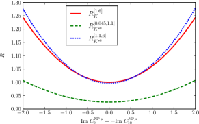
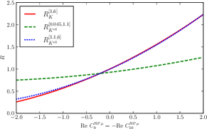
(a)	(b)

Figure 1: Values of $R_{K}$ and $R_{K^{*0}}$ with (a) imaginary and (b) real Wilson coefficients.

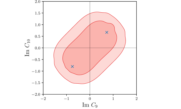
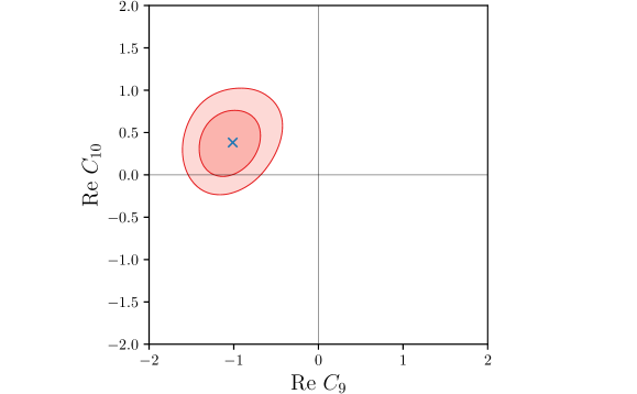
(a)	(b)

Figure 2: Best fit and $1\,\sigma$ and $2\,\sigma$ contours to semi-leptonic $B$-decays observables, $R_{K},R_{K^{*0}},P_{4}^{\prime}$ and $P_{5}^{\prime}$, using (a) imaginary and (b) real Wilson coefficients.

We have done a global fit by including the ratios $R_{K}$ and $R_{K^{*0}}$, and the angular observables $P_{4}^{\prime}$ and $P_{5}^{\prime}$ [6, 19, 21, 22]. Results are shown in Figure 2. The allowed regions for imaginary values of $C_{9}^{\rm{NP}\,\mu}$ and $C_{10}^{\rm{NP}\,\mu}$ when fitting to measurements of a series of $b\to s\mu^{+}\mu^{-}$ observables are presented in Figure 2a, by assuming all other Wilson coefficients to be SM-like. The numerical analysis has been done by using the open source code flavio 0.28 [55], which computes the $\chi^{2}$ function with each $(C_{9}^{\rm{NP}\,\mu},C_{10}^{\rm{NP}\,\mu})$ pair. The $\chi^{2}$ difference is evaluated with respect to the SM point, $\Delta\chi^{2}_{\mathrm{SM}}=\chi^{2}_{\mathrm{SM}}-\chi^{2}_{\mathrm{min}}$. Then, the pull in $\sigma$ is defined as $\sqrt{\Delta\chi^{2}_{\mathrm{SM}}}$, in the case of only one Wilson coefficient, and for the two-dimensional case it can be evaluated by using the inverse cumulative distribution function of a $\chi^{2}$ distribution having two degrees of freedom; for instance, $\Delta\chi^{2}=2.29$ for $1\,\sigma$. The darker red shaded regions in Fig. 2 correspond to the points with $\Delta\chi^{2}=\chi^{2}-\chi^{2}_{\mathrm{min}}\leq 2.29$, that is, they are less than $1\,\sigma$ away from the best fit point, whereas the lighter red shaded regions correspond to $\Delta\chi^{2}\leq 6.18$ ($\equiv 2\,\sigma$). The crosses mark the position of the best fit points. In Fig. 2a the $\chi^{2}$ function has a broad flat region centered around the origin, with two nearly symmetric minima found at ($C_{9}^{\rm{NP}\,\mu}=0.72\,i$, $C_{10}^{\rm{NP}\,\mu}=0.74\;i$) and ($C_{9}^{\rm{NP}\,\mu}=-0.75\,i$, $C_{10}^{\rm{NP}\,\mu}=-0.74\,i$). The pull of the SM, defined as the probability that the SM scenario can describe the best fit assuming that $\Delta\chi^{2}_{\mathrm{SM}}$ follows a $\chi^{2}$ distribution with 2 degrees of freedom, is of just $\sqrt{\Delta\chi^{2}_{\mathrm{SM}}}=1.42$ ($\equiv 0.91\,\sigma$) and $\sqrt{\Delta\chi^{2}_{\mathrm{SM}}}=1.38$ ($\equiv 0.87\,\sigma$) respectively, and both of them have the same $\chi^{2}_{\mathrm{min}}/\mathrm{d.o.f.}=2.25$, that is, purely complex couplings do not provide a good description of the data. For completeness, the fit to real values of the Wilson coefficients are included in Figure 2b. Now the confidence regions are much tighter and do not include the SM point. In fact, the best fit point ($C_{9}^{\rm{NP}\,\mu}=-1.09$, $C_{10}^{\rm{NP}\,\mu}=0.481$) improves the SM by $\sqrt{\Delta\chi^{2}_{\mathrm{SM}}}=6.28$ ($\equiv 5.95\,\sigma$), and a much lower $\chi^{2}_{\mathrm{min}}/\mathrm{d.o.f.}=1.24$.

Ref. [26] showed that imaginary Wilson coefficients do not interfere with the SM amplitude, an therefore imaginary $C_{9,10}^{\rm{NP}\,\mu}$ can not decrease the prediction for $R_{K}$, $R_{K^{*0}}$. This is numerically shown in the above analysis, where imaginary Wilson coefficients $C_{9,10}^{\rm{NP}\,\mu}$ are not able to reduce significantly the prediction for $R_{K}$, $R_{K^{*0}}$. To further investigate this question we have analytically computed a numerical approximation to $R_{K^{*0}}$ as a function of $C_{9}^{\rm{NP}\,\mu}$, $C_{10}^{\rm{NP}\,\mu}$ in the region $1.1\leq q^{2}\leq 6.0\,{\rm GeV}^{2}$. After integration and some approximations regarding the scalar products of final state momenta, we obtain:

$$R_{K^{*0}}\simeq\frac{0.9875+0.1759\,\mathrm{Re}\,C_{9}^{\rm{NP}\,\mu}-0.2954\,\mathrm{Re}\,C_{10}^{\rm{NP}\,\mu}+0.0212|C_{9}^{\rm{NP}\,\mu}|^{2}+0.0350|C_{10}^{\rm{NP}\,\mu}|^{2}}{1\,\ \ \ \ \ +0.1760\,\mathrm{Re}\,C_{9}^{\rm{NP}\,e}-0.3013\,\mathrm{Re}\,C_{10}^{\rm{NP}\,e}+0.0212|C_{9}^{\rm{NP}\,e}|^{2}+0.0357|C_{10}^{\rm{NP}\,e}|^{2}}\ \ \ \ \ \ \ \$$

$$(1.1\leq q^{2}\leq 6.0\,{\rm GeV}^{2}).$$ (17)

We have checked that this approximation reproduces the flavio-computed value of $R_{K^{*0}}$ to better than $4\%$ in a large region of the parameter space. Now, if we assume that NP does not affect the electron channel ($C_{9}^{\rm{NP}\,e}=C_{10}^{\rm{NP}\,e}=0$), it is clear that to obtain $R_{K^{*0}}<R_{K^{*0}}^{\mathrm{SM}}$ one needs to introduce $C_{9}^{\rm{NP}\,\mu}$ and $C_{10}^{\rm{NP}\,\mu}$ with a non-zero real part: the only possible negative contributions come from the $\mathrm{Re}\,C_{9}^{\rm{NP}\,\mu}$, $\mathrm{Re}\,C_{10}^{\rm{NP}\,\mu}$ terms, whereas the $|C_{9}^{\rm{NP}\,\mu}|^{2}$, $|C_{10}^{\rm{NP}\,\mu}|^{2}$ terms have a positive-defined sign, and can not reduce the value of $R_{K^{*0}}$. Thus, purely imaginary values of $C_{9,10}^{\rm{NP}\,\mu}$ contribute only to the modulus (positive-definite) and not to the real part, and can not bring the prediction of $R_{K^{*0}}$ closer to the experimental value. In addition, this expression tells us that the better option to reduce the prediction of $R_{K^{*0}}$ is using a real negative $C_{9}^{\rm{NP}\,\mu}$, and a real positive $C_{10}^{\rm{NP}\,\mu}$. This is actually the result that we have obtained in our numerical analysis. Fig. 1b shows that, for real Wilson coefficients, the lowest prediction for $R_{K^{*0}}$  is obtained for $C_{9}^{\rm{NP}\,\mu}=-C_{10}^{\rm{NP}\,\mu}<0$, and Fig.2b shows that the best fit is obtained for negative $C_{9}^{\rm{NP}\,\mu}$ and positive $C_{10}^{\rm{NP}\,\mu}$. Fig. 1a shows that, in general, imaginary Wilson coefficients give positive contributions to $R_{K}$, $R_{K^{*0}}$, in accordance with eq. (17). Of course, the full expression is richer than eq. (17), and we expect some deviations, Fig. 2a shows that the best fit point is not the SM ($C_{9}^{\rm{NP}\,\mu}=C_{10}^{\rm{NP}\,\mu}=0$), but the best fit regions are centered around it, and the SM pull with respect the best fit points is small.

	Best fit(s)	Pull ($\sqrt{\Delta\chi^{2}_{\mathrm{SM}}}$)	Pull ($\sigma$)	$\chi^{2}_{\mathrm{min}}/\mathrm{d.o.f.}$
$C_{9}^{\rm{NP}\,\mu}$	$-1.11-0.02\;i$	5.94	5.60 $\sigma$	1.35
$C_{10}^{\rm{NP}\,\mu}$	$1.66+1.99\;i$	5.02	4.65 $\sigma$	1.62
	$1.67-2.01\;i$
$C_{9}^{\rm{NP}\,\mu}=-C_{10}^{\rm{NP}\,\mu}$	$-1.16+1.14\;i$	6.06	5.72 $\sigma$	1.31
	$-1.18-1.18\;i$
$C_{9}^{{}^{\prime}\rm{NP}\,\mu}$	$-0.24-0.003\;i$	1.07	0.57 $\sigma$	2.27
$C_{10}^{{}^{\prime}\rm{NP}\,\mu}$	$0.33-0.014\;i$	2.22	1.72 $\sigma$	2.17
$C_{9}^{\rm{NP}\,e}$	$-3.29+5.02\;i$	4.85	4.47 $\sigma$	1.67
	$-3.35-5.04\;i$
$C_{10}^{\rm{NP}\,e}$	$-0.27+3.48\;i$	4.72	4.34 $\sigma$	1.70
	$-0.27-3.48\;i$
$C_{9}^{\rm{NP}\,e}=-C_{10}^{\rm{NP}\,e}$	$-3.29+4.58\;i$	4.85	4.47 $\sigma$	1.67
	$-3.35-4.59\;i$
$C_{9}^{{}^{\prime}\rm{NP}\,e}$	$-0.59+3.89\;i$	4.81	4.43 $\sigma$	1.68
	$-0.59-3.89\;i$
$C_{10}^{{}^{\prime}\rm{NP}\,e}$	$0.52+3.88\;i$	4.81	4.43 $\sigma$	1.68
	$0.53-3.88\;i$

Table 1: Best fit Wilson coefficients complex values to semi-leptonic decay observables $R_{K},R_{K^{*0}},P_{4}^{\prime}$ and $P_{5}^{\prime}$, allowing only one free coefficient at a time. Shown are also the corresponding pulls, and $\chi^{2}_{\mathrm{min}}/\mathrm{d.o.f.}$.

	$R_{K}$	$R_{K^{*0}}^{[0.045,1.1]}$	$R_{K^{*0}}^{[1.1,6]}$
$C_{9}^{\rm{NP}\,\mu}$	$0.77\pm 0.03$	$0.887\pm 0.009$	$0.82\pm 0.04$
$C_{10}^{\rm{NP}\,\mu}$	$0.78\pm 0.05$	$0.87\pm 0.03$	$0.80\pm 0.10$
$C_{9}^{\rm{NP}\,\mu}=-C_{10}^{\rm{NP}\,\mu}$	$0.59\pm 0.08$	$0.83\pm 0.03$	$0.63\pm 0.09$
$C_{9}^{{}^{\prime}\rm{NP}\,\mu}$	$0.95\pm 0.05$	$0.96\pm 0.03$	$1.09\pm 0.09$
$C_{10}^{{}^{\prime}\rm{NP}\,\mu}$	$0.92\pm 0.07$	$0.95\pm 0.03$	$1.07\pm 0.09$
$C_{9}^{\rm{NP}\,e}$	$0.76\pm 0.09$	$0.69\pm 0.12$	$0.52\pm 0.17$
$C_{10}^{\rm{NP}\,e}$	$0.69\pm 0.06$	$0.77\pm 0.06$	$0.59\pm 0.13$
$C_{9}^{\rm{NP}\,e}=-C_{10}^{\rm{NP}\,e}$	$0.76\pm 0.09$	$0.70\pm 0.10$	$0.52\pm 0.17$
$C_{9}^{{}^{\prime}\rm{NP}\,e}$	$0.75\pm 0.09$	$0.71\pm 0.10$	$0.52\pm 0.18$
$C_{10}^{{}^{\prime}\rm{NP}\,e}$	$0.75\pm 0.09$	$0.80\pm 0.09$	$0.66\pm 0.14$

Table 2: $R_{K}$, $R_{K^{*0}}$ predictions with $1\,\sigma$ uncertainties corresponding to the best fit Wilson coefficients of Table 1.

We conclude that, actually, a NP explanation for $R_{K}$, $R_{K^{*0}}$ requires that $C_{9}^{\rm{NP}\,\mu}$, $C_{10}^{\rm{NP}\,\mu}$  have a non-zero real part, whereas we saw above that NP explanation for $\Delta M_{s}$  requires that $C_{9}^{\rm{NP}\,\mu}$, $C_{10}^{\rm{NP}\,\mu}$ have a non-zero imaginary part. Then, to have a NP explanation for both observables $C_{9}^{\rm{NP}\,\mu}$, $C_{10}^{\rm{NP}\,\mu}$  should be general complex numbers. Following this reasoning we have performed a global fit to the semi-leptonic decay observables $R_{K},R_{K^{*0}},P_{4}^{\prime}$ and $P_{5}^{\prime}$ using generic complex Wilson coefficients allowing only one free Wilson coefficient at a time. Table 1 shows the best fit values, pulls (defined as $\sqrt{\Delta\chi^{2}_{\mathrm{SM}}}$) and $\chi^{2}_{\mathrm{min}}/\mathrm{d.o.f.}$, for scenarios with NP in one individual complex Wilson coefficient, and Table 2 shows the prediction for $R_{K}$, $R_{K^{*0}}$ for the corresponding central values of each fit, together with the $1\,\sigma$ uncertainties. The primed Wilson coefficients are also included. We found that the best fit of $R_{K}$ and $R_{K^{*0}}$ and the angular distributions is obtained for $C_{9}^{\rm{NP}\,\mu}=-1.11-0.02\;i$, for $C_{10}^{\rm{NP}\,\mu}$ we find two points with similar minimum value for $\chi^{2}$ with opposite signs of the imaginary part, $C_{10}^{\rm{NP}\,\mu}=1.66+1.99\;i$ and $C_{10}^{\rm{NP}\,\mu}=1.65-2.10\;i$. Assuming $C_{9}^{\rm{NP}\,\mu}=-C_{10}^{\rm{NP}\,\mu}$ we also obtain a double minimum $C_{9}^{\rm{NP}\,\mu}=-C_{10}^{\rm{NP}\,\mu}=-1.16+1.14\;i$ and $C_{9}^{\rm{NP}\,\mu}=-C_{10}^{\rm{NP}\,\mu}=-1.18-1.18\;i$ with a pull of $\sqrt{\Delta\chi^{2}_{\mathrm{SM}}}=6.06$ ($\equiv 5.72\,\sigma$) and a $\chi^{2}_{\mathrm{min}}/\mathrm{d.o.f.}=1.31$. By looking at $\chi^{2}_{\mathrm{min}}/\mathrm{d.o.f.}$ we see that the scenarios with only $C_{9}^{\rm{NP}\,\mu}$ or $C_{9}^{\rm{NP}\,\mu}=-C_{10}^{\rm{NP}\,\mu}$ provide the best description of experimental data, whereas the scenarios with $C_{9}^{{}^{\prime}\rm{NP}\,\mu}$ and $C_{10}^{{}^{\prime}\rm{NP}\,\mu}$ provide the worst description. If only real Wilson coefficients are chosen the best fit of $R_{K}$ and $R_{K^{*0}}$ yields $C_{9}^{\rm{NP}\,\mu}=-1.59$, $C_{10}^{\rm{NP}\,\mu}=1.23$ or $C_{9}^{\rm{NP}\,\mu}=-C_{10}^{\rm{NP}\,\mu}=-0.64$, with a pull around $4.2\,\sigma$ [36].

Ref.[34] also provides fits for complex generic Wilson coefficients. Their scenario I corresponds to our first line in Table 1, our best fit value agrees with their result ($C_{9}^{\rm{NP}\,\mu}=(-1.1\pm 0.2)+(0\pm 0.9\,i)$), within the large uncertainties they give for the imaginary part, but we obtain larger pulls ($5.6\,\sigma$ vs. $4.2\,\sigma$ of Ref.[34]). Their scenario II corresponds to our third line in Table 1 ($C_{9}^{\rm{NP}\,\mu}=-C_{10}^{\rm{NP}\,\mu}$), we agree with the main features of their fit, for the real part they obtain $\mathrm{Re}(C_{9}^{\rm{NP}\,\mu})=\mathrm{Re}(C_{10}^{\rm{NP}\,\mu})=-0.8\pm 0.3$, we obtain a slightly smaller real part, but they agree within uncertainties, both of us obtain a double minimum for the imaginary part $\sim\pm(1.1-1.2)\,i$, again, we obtain a slightly larger pull ($5.72\,\sigma$ vs. $4.0$, $4.2\,\sigma$ of Ref.[34]).

Choosing complex Wilson coefficients also implies additional constraints from $CP$-violating observables. This fact has not been considered in the previous analysis. In the next section we study the consequences of having these coefficients in the analysis of $B$-meson anomalies on some NP models and we consider a global fit of both the ratios $R_{K}$ and $R_{K^{*0}}$ and the angular observables $P_{4}^{\prime}$ and $P_{5}^{\prime}$, and also the $CP$-mixing asymmetry.

4 $B_{s}$-mixing and NP models

Several NP models that are able to explain the lepton flavour universality violation effects are constrained by other flavour observables like $B_{s}$-mixing. In particular the parameter space of $Z^{{}^{\prime}}$ and leptoquark models are severely constrained by the present experimental results of $\Delta M_{s}$ [47]. Besides, as already mentioned, additional constraints emerge from $CP$-violating observables when considering complex couplings. Ref.[47] argues that nearly imaginary Wilson coefficients could explain the discrepancies with the $\Delta M_{s}$ experimental measurement, but a global fit of $R_{K}$ and $R_{K^{*0}}$ observables, together with $\Delta M_{s}$ and $CP$-violation observable $A_{CP}^{\rm{mix}}$ in $B_{s}\rightarrow J/\psi\phi$ decays should be performed. In the next subsections we investigate these issues for the case of $Z^{{}^{\prime}}$ and leptoquark models.

4.1 $Z^{{}^{\prime}}$ fit

From now on, a global fit of $R_{K}$ and $R_{K^{*0}}$ observables, $\Delta M_{s}$ and the $CP$-violation observable $A_{CP}^{\rm{mix}}$ is included in our analysis.

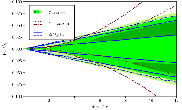
Figure 3: Fit on $Z^{\prime}$ parameter space in the $M_{Z^{\prime}}$-Im $\lambda_{23}^{Q}$ plane (see text).

Figure 3 shows the fits on the $Z^{\prime}$ mass $M_{Z^{\prime}}$ and the imaginary coupling $\lambda_{23}^{Q}$ (setting $\lambda_{22}^{L}=1$) imposed by $b\to s\mu^{+}\mu^{-}$ decays and $B_{s}$-mixing. The red lines (dotted, dash-dotted) correspond to the fit using only semi-leptonic $B$-meson decays, i.e. $b\to s\mu^{+}\mu^{-}$ as in Figure 2 plus the branching ratios $\mathrm{BR}(B_{s}\to\mu^{+}\mu^{-})$ and $\mathrm{BR}(B^{0}\to\mu^{+}\mu^{-})$. The best fit region is the one between the curves; dotted lines: $\Delta\chi^{2}=1$, dash-dotted lines: $\Delta\chi^{2}=4$. Blue lines (solid, dashed) correspond to the fit to $B_{s}$-mixing observables $\Delta M_{s}$ and $A_{CP}^{\rm{mix}}$. The best fit region is the one between the lines; solid lines $\Delta\chi^{2}=1$, dashed lines $\Delta\chi^{2}=4$, there are two regions with $\Delta\chi^{2}<1$, but between them $\Delta\chi^{2}$ is always smaller than 4. The green regions are the combined global fit: dark region $\Delta\chi^{2}\leq 1$, medium $\Delta\chi^{2}\leq 4$ and light $\Delta\chi^{2}\leq 9$.

Best fits	Real	Imaginary	Complex
$\lambda_{23}^{Q}$	$-0.002$	$\pm 0.047\;i$	$-0.0020-0.0021\;i$
$M_{Z^{\prime}}$	1.31 TeV	12 TeV	1.08 TeV
Pull ($\sqrt{\Delta\chi^{2}_{\mathrm{SM}}}$)	5.70	1.61	6.05
Pull ($\sigma$)	5.39 $\sigma$	1.09 $\sigma$	5.43 $\sigma$
$\chi^{2}_{\mathrm{min}}/\mathrm{d.o.f.}$	1.41	2.12	1.34
$R_{K}$	$0.66\pm 0.05$	$1.00\pm 0.01$	$0.65\pm 0.07$
$R_{K^{*0}}^{[0.045,1.1]}$	$0.849\pm 0.013$	$0.93\pm 0.02$	$0.84\pm 0.02$
$R_{K^{*0}}^{[1.1,6]}$	$0.68\pm 0.05$	$1.00\pm 0.01$	$0.68\pm 0.07$
$\Delta M_{s}$	$20.41\pm 1.26$ ps-1	$18.0\pm 1.7$ ps-1	$19.95\pm 1.27$ ps-1
$A_{CP}^{\rm{mix}}$	$-0.0369\pm 0.0002$	$-0.041\pm 0.002$	$-0.035\pm 0.003$

Table 3: Best fits, and corresponding pulls, to $R_{K},R_{K^{*0}},\Delta M_{s}$ and $A_{CP}^{\rm{mix}}$; considering real, imaginary and complex Wilson coefficients on the $Z^{{}^{\prime}}$ model. Shown are also the corresponding pulls, $\chi^{2}_{\mathrm{min}}/\mathrm{d.o.f.}$, and the predictions for semi-leptonic decay observables $R_{K}$, $R_{K^{*0}}$; $\Delta M_{s}$ and $A_{CP}^{\rm{mix}}$ with $1\,\sigma$ uncertainties.

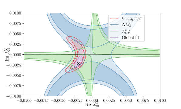
Figure 4: Fit on $Z^{\prime}$ parameter space in the $\lambda_{23}^{Q}$ complex plane for the best fit $Z^{\prime}$ mass $M_{Z^{\prime}}=1.08\,{\rm TeV}$ (see text).

The best fit for the $b\to s\mu^{+}\mu^{-}$ observables in the region under study is $M_{Z^{\prime}}=11\,{\rm TeV}$, $\lambda_{23}^{Q}=0.015\;i$, with a tiny $\sqrt{\Delta\chi^{2}_{\mathrm{SM}}}=0.23$, which makes it statistically indistinguishable from the SM, and a large $\chi^{2}_{\mathrm{min}}/\mathrm{d.o.f.}=2.92$ which indicates that it does not provide a good fit to the data. For the $B_{s}$-mixing observables, the best fit is found at the maximum allowed mass $M_{Z^{\prime}}=12\,{\rm TeV}$, $\lambda_{23}^{Q}=\pm 0.05\;i$, which corresponds to $C_{bs}^{LL}=-1.54\times 10^{-4}$. The SM has a pull of $\sqrt{\Delta\chi^{2}_{\mathrm{SM}}}=1.73$ ($\equiv 1.21\,\sigma$), and the minimum has a $\chi^{2}_{\mathrm{min}}/\mathrm{d.o.f.}=0.52$. The best fit when all observables are considered, in the $M_{Z^{\prime}}$ region of our analysis, and $\lambda_{23}^{Q}$ being a pure imaginary coupling, is found at $M_{Z^{\prime}}=12\,{\rm TeV}$, $\lambda_{23}^{Q}=\pm 0.047\;i$, and the pull of the SM is $\sqrt{\Delta\chi^{2}_{\mathrm{SM}}}=1.61(\equiv 1.09\,\sigma)$ and $\chi^{2}_{\mathrm{min}}/\mathrm{d.o.f.}=2.12$. Larger values of $M_{Z^{\prime}}$ do not improve the pull of the SM. Actually, if one allows larger values for $M_{Z^{\prime}}$ the best fit point has a linear relation between the coupling and the maximal allowed mass: $\lambda_{23}^{Q}\simeq i\,(3.95\times M_{Z^{\prime}}^{\mathrm{max}}/\,{\rm TeV})\times 10^{-3}$. This linear relation produces a (approximately) constant $C_{bs}^{LL}$ (12), with a $\Delta M_{s}$ prediction close to the experimental value (2), while the contributions to $|C_{9,10}^{\rm{NP}\,\mu}|$ decrease as $M_{Z^{\prime}}^{-1}$ (11). Since imaginary couplings worsen the $R_{K}$, $R_{K^{*0}}$ prediction, the larger $M_{Z^{\prime}}$ provides better predictions for them, bringing them closer to the SM value. The best fit $\Delta\chi^{2}_{\mathrm{SM}}$ grows very slowly with growing allowed $M_{Z^{\prime}}$. Table 3 summarizes the best fit values for $\lambda_{23}^{Q}$ and $M_{Z^{\prime}}$, and corresponding pulls, to $R_{K}$ and $R_{K^{*0}}$ observables, $\Delta M_{s}$ and $A_{CP}^{\rm{mix}}$; considering real, imaginary and complex Wilson coefficients. Results for the above observables in each scenario are included in this table. It is clear that $R_{K}$ and $R_{K^{*0}}$ observables prefer real Wilson coefficients, as expected. For real couplings the description is better than the SM, with a pull of $5.39\,\sigma$ but it does not improve the prediction for $\Delta M_{s}$. Contrary, to improve the prediction for $\Delta M_{s}$ imaginary couplings are required in the $Z^{{}^{\prime}}$ model, however the pull with respect the SM is small, and it has a large $\chi^{2}_{\mathrm{min}}/\mathrm{d.o.f.}$. When allowing generic complex couplings (third column in Table 3) we find that the best fit point is close to the best fit point using only real couplings (first column in Table 3), and the pull with respect the SM improves slightly ($5.43\,\sigma$ versus $5.39\,\sigma$), and the predictions for the observables are also close to the pure real couplings case, showing a slight improvement in the prediction for $\Delta M_{s}$.

Fig. 4 shows the best fit regions in the complex $\lambda_{23}^{Q}$ plane for the best fit mass value $M_{Z^{\prime}}=1.08\,{\rm TeV}$ (Table 3). The red region shows the 2-dimensional 1 and 2-$\sigma$ allowed values ($\Delta\chi^{2}=2.29$, $6.18$) including only the $b\to s\mu^{+}\mu^{-}$ observables, the blue region shows the 1 and 2-$\sigma$ allowed values including only $\Delta M_{s}$, and the green region show the 1 and 2-$\sigma$ allowed values including only $A_{CP}^{\rm{mix}}$, the violet region shows the combined fit. Here we see the tension between the $b\to s\mu^{+}\mu^{-}$ and $\Delta M_{s}$ fits. $b\to s\mu^{+}\mu^{-}$ selects a region around the real axis of the coupling, whereas $\Delta M_{s}$ selects regions away from it. There are two small intersection regions for the 1-$\sigma$ allowed values of both fits. The $A_{CP}^{\rm{mix}}$ fit selects one of these regions, and breaks the degeneracy. Actually, the $b\to s\mu^{+}\mu^{-}$ fit selects fixed values of $C_{9}^{\rm{NP}\,\mu}=-C_{10}^{\rm{NP}\,\mu}$, eq. (11), since $C_{9}^{\rm{NP}\,\mu}=-C_{10}^{\rm{NP}\,\mu}$ scale as $\sim\lambda_{23}^{Q}/M_{Z^{\prime}}^{2}$, for fixed $C_{9}^{\rm{NP}\,\mu}=-C_{10}^{\rm{NP}\,\mu}$ the allowed values of $\lambda_{23}^{Q}$ (red region in Fig. 4) around the real axis will grow as $M_{Z^{\prime}}^{2}$, but, at the same time, the allowed region will move away from the imaginary axis as $M_{Z^{\prime}}^{2}$. On the other hand, the fit on $\Delta M_{s}$ selects fixed values of $C_{bs}^{LL}$, eq. (12), since $C_{bs}^{LL}\sim(\lambda_{23}^{Q})^{2}/M_{Z^{\prime}}^{2}$, for fixed $C_{bs}^{LL}$ the 1-$\sigma$ unfavored region around the origin (light blue region in Fig. 4) will grow as $\lambda_{23}^{Q}\sim M_{Z^{\prime}}$. As $M_{Z^{\prime}}$ grows, the red region moves away from the origin as $M_{Z^{\prime}}^{2}$, but the blue region expands only as $M_{Z^{\prime}}$, so that at some $M_{Z^{\prime}}$ value their 1-$\sigma$ regions do not longer intersect. This is the reason why we obtain a relatively low $M_{Z^{\prime}}$ in the fits of Table 3.

Ref.[34] provides also a fit for the $Z^{\prime}$ model, using a fixed $M_{Z^{\prime}}=1\,{\rm TeV}$, this value is close to our best fit value of Table 3. For $\lambda_{22}^{L}=1$ they obtain the best fit coupling $\lambda_{23}^{Q}=(-0.8\pm 0.3)\times 10^{-3}+(-0.4\pm 3.1)\times 10^{-3}\,i$ with a pull of $4.0\,\sigma$. Our best fit values agree with them within uncertainties. Note that we do not provide uncertainties for the best fit values, the reason being that the parameters are not independent, the 2-dimensional best fit regions in Fig. 4 are not ellipses, and the best fit points are not on the center of the figures, so that giving a central value with 1-dimensional uncertainties overestimates the uncertainty and leads to confusion about the meaning and position of the best fit point.

We conclude that, in the framework of $Z^{\prime}$ models, $R_{K}-R_{K^{*0}}$ observables are better described than in the SM, with a pull $\stackrel{{\scriptstyle\scriptstyle>}}{{{}_{\sim}}}5.39\,\sigma$ for $M_{Z^{\prime}}\simeq 1-1.3\,{\rm TeV}$, and a coupling with a real part ${\rm Re}(\lambda_{23}^{Q})\simeq-0.002$. The presence of a similar imaginary part for the coupling ${\rm Im}(\lambda_{23}^{Q})\simeq-0.0021$ improves slightly the fit, as well as the $\Delta M_{s}$ prediction.

4.2 Leptoquark fit

Figure 5: Fit on $S_{3}$ leptoquark parameter space in the $M_{S_{3}}$-Im $y^{QL}_{32}y^{QL*}_{22}$ plane (see text).

The leptoquark model has three independent couplings contributing to $\Delta M_{s}$ (15). For the global fits we will assume that the dominant coupling is the muon coupling $y^{QL}_{32}y^{QL*}_{22}$, which is the one contributing to $R_{K}$, $R_{K^{*0}}$ (14). The fits on the $S_{3}$ leptoquark mass $M_{S_{3}}$ and the imaginary coupling $y^{QL}_{32}y^{QL*}_{22}$ imposed by $b\to s\mu^{+}\mu^{-}$ decays and $B_{s}$-mixing are presented in Figure 5. The observables used in the respective fits are the same as in Figure 3. The red lines (dotted, dash-dotted) correspond to the fit using only semi-leptonic $B$-meson decays, i.e. $b\to s\mu^{+}\mu^{-}$ plus the branching ratios $\mathrm{BR}(B_{s}\to\mu^{+}\mu^{-})$ and $\mathrm{BR}(B^{0}\to\mu^{+}\mu^{-})$, the best fit region is the one between the curves; dotted lines: $\Delta\chi^{2}=1$, dash-dotted lines: $\Delta\chi^{2}=4$. Blue lines (solid, dashed) correspond to the fit to $B_{s}$-mixing observables $\Delta M_{s}$ and $A_{CP}^{\rm{mix}}$. The best fit region is the one between the lines; solid lines $\Delta\chi^{2}=1$, dashed lines $\Delta\chi^{2}=4$, there are two regions with $\Delta\chi^{2}<1$, but between them $\Delta\chi^{2}$ is always smaller than 4. The green regions are the combined global fit: dark region $\Delta\chi^{2}\leq 1$, medium $\Delta\chi^{2}\leq 4$ and light $\Delta\chi^{2}\leq 9$. In the $b\to s\mu^{+}\mu^{-}$ fit the best fit parameters for imaginary couplings is $y_{32}^{QL}y_{22}^{QL*}=-0.2\,i$, $M_{S_{3}}=40.8\,{\rm TeV}$. The leptoquark fit to $B_{s}$-mixing observables has a double minimum, located at $M_{S_{3}}=44.9\,{\rm TeV}$, $y_{32}^{QL}y_{22}^{QL*}=\pm 2\;i$, with a SM pull of $\sqrt{\Delta\chi^{2}_{\mathrm{SM}}}=1.74$ ($\equiv 1.22\,\sigma$) and $\chi^{2}_{\mathrm{min}}/\mathrm{d.o.f.}=0.51$. These points correspond to a value for the Wilson coefficient of $C_{bs}^{LL}=-1.39\times 10^{-4}$. The global fit, including all observables, and considering only imaginary $y_{32}^{QL}y_{22}^{QL*}$ couplings, is located at $M_{S_{3}}=50\,{\rm TeV}$, $y_{32}^{QL}y_{22}^{QL*}=-1.67\;i$; with a SM pull of only $\sqrt{\Delta\chi^{2}_{\mathrm{SM}}}=1.1(\equiv 0.6\,\sigma)$ and a large $\chi^{2}_{\mathrm{min}}/\mathrm{d.o.f.}=2.16$. Larger $M_{S_{3}}$ masses provide similar values for the best fit couplings, and observable predictions, and the pulls improve slowly. The situation is similar than in the $Z^{\prime}$ case: by allowing larger $M_{S_{3}}$ masses the best fit coupling reaches an asymptotic straight line, where the contribution to $\Delta M_{s}$ is constant (15), whereas the contribution to $|C_{9,10}^{\rm{NP}\,\mu}|$ (14) decreases as $M_{S_{3}}^{-1}$, the best fit coupling behaves as $y_{32}^{QL}y_{22}^{QL*}\simeq i\,(4.43\times 10^{-2}\times M_{S_{3}}/\,{\rm TeV})$. Table 4 shows the best fit parameters for the leptoquark model considered in this work, corresponding pulls, predictions to the observables $R_{K}$, $R_{K^{*0}}$, $\Delta M_{s}$ and $A_{CP}^{\rm{mix}}$ and $\chi^{2}_{\mathrm{min}}/\mathrm{d.o.f.}$, considering real, imaginary and complex Wilson coefficients. Table 4 shows that only imaginary couplings do not improve the results, they cannot explain the $R_{K^{(*)}}$ anomaly. However, when complex couplings are considered, we found a better global fit of $R_{K},R_{K^{*0}}$ observables, the best global fit parameters emerge at $M_{S_{3}}=4.1\,{\rm TeV}$ and $y_{32}^{QL}y_{22}^{QL*}=0.033+0.034\;i$, with $\sqrt{\Delta\chi^{2}_{\mathrm{SM}}}=5.90$ ($\equiv 5.27\,\sigma$). The best fit point $M_{S_{3}}$ and the coupling real part are similar to the real couplings case. The imaginary part of the coupling is similar to the real part. The pull with respect the SM is marginally better in the case of complex couplings ($\sqrt{\Delta\chi^{2}_{\mathrm{SM}}}=5.9$ versus $5.82$), but it actually worsens in units of $\sigma$, since the complex coupling fit has one more free parameter. The $\chi^{2}_{\mathrm{min}}/\mathrm{d.o.f.}$ is similar in both scenarios. The predictions for the $B$-meson physics observables are similar than in the real couplings case.

Best fits	Real	Imaginary	Complex
$y^{QL}_{32}y^{QL*}_{22}$	$0.04$	$-1.67\;i$	$0.033+0.034\;i$
$M_{S_{3}}$	5.19 TeV	50 TeV	4.10 TeV
Pull ($\sqrt{\Delta\chi^{2}_{\mathrm{SM}}}$)	5.82	1.10	5.90
Pull ($\sigma$)	5.47 $\sigma$	0.60 $\sigma$	5.27 $\sigma$
$\chi^{2}_{\mathrm{min}}/\mathrm{d.o.f.}$	1.38	2.16	1.39
$R_{K}$	$0.64\pm 0.06$	$1.00\pm 0.01$	$0.62\pm 0.14$
$R_{K^{*0}}^{[0.045,1.1]}$	$0.835\pm 0.015$	$0.93\pm 0.02$	$0.84\pm 0.04$
$R_{K^{*0}}^{[1.1,6]}$	$0.66\pm 0.06$	$1.00\pm 0.01$	$0.66\pm 0.14$
$\Delta M_{s}$	$20.07\pm 1.27$ ps-1	$18.8\pm 1.7$ ps-1	$20.0\pm 1.2$ ps-1
$A_{CP}^{\rm{mix}}$	$-0.0374\pm 0.0006$	$-0.039\pm 0.002$	$-0.032\pm 0.003$

Table 4: Best fits, and corresponding pulls, to $R_{K},R_{K^{*0}},\Delta M_{s}$ and $A_{CP}^{\rm{mix}}$; considering real, imaginary and complex Wilson coefficients on the $S_{3}$ leptoquark. Shown are also the corresponding pulls, $\chi^{2}_{\mathrm{min}}/\mathrm{d.o.f.}$ and the predictions for semi-leptonic decay observables $R_{K}$, $R_{K^{*0}}$; $\Delta M_{s}$ and $A_{CP}^{\rm{mix}}$ with $1\,\sigma$ uncertainties.

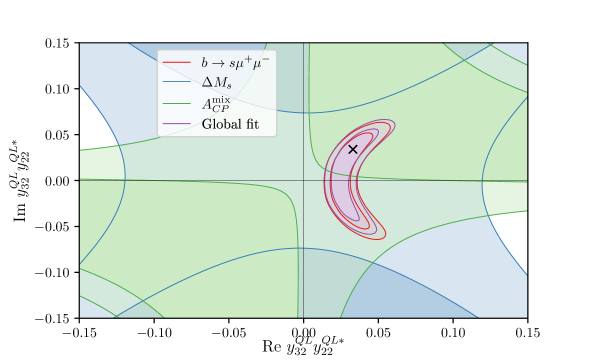
Figure 6: Fit on $S_{3}$ leptoquark parameter space in the complex $y^{QL}_{32}y^{QL*}_{22}$ plane for the best fit leptoquark mass $M_{S_{3}}=4.1\,{\rm TeV}$ (see text).

Fig. 6 shows the best fit regions in the complex $y_{32}^{QL}y_{22}^{QL*}$ plane, for the best fit mass parameter $M_{S_{3}}=4.1\,{\rm TeV}$, Table 4. The meaning of each region is as in Fig. 4. In this model there is no intersection between the 1-$\sigma$ best fit regions of the $b\to s\mu^{+}\mu^{-}$ and the $\Delta M_{s}$ fits. Here we also find the tension between the $b\to s\mu^{+}\mu^{-}$ and $\Delta M_{s}$ observables, and the different evolution of the best fit regions with the leptoquark mass $M_{S_{3}}$. The $\Delta M_{s}$ fit moves the best fit point away from the real axis, and the $A_{CP}^{\rm{mix}}$ fit selects of the of the signs for the imaginary part, however the global best fit region lies outside the 1-$\sigma$ region for $\Delta M_{s}$, and the $\Delta M_{s}$ prediction does not improve with respect the SM.

Ref.[34] also provides a fit for the leptoquark scenario, our model corresponds to their $\vec{\Delta}_{1/3}[S3]$ model. Ref.[34] performs a fit fixing the leptoquark mass to $M_{S_{3}}=1\,{\rm TeV}$, and they obtain a two nearly degenerate minimums with positive and negative imaginary parts. The reason for that is that they do not include the $A_{CP}^{\rm{mix}}$ observable in the fit. Since the $C_{9}^{\rm{NP}\,\mu}=-C_{10}^{\rm{NP}\,\mu}$ Wilson coefficient scales like $\sim y_{32}^{QL}y_{22}^{QL*}/M_{S_{3}}^{2}$ (14) we can compare both results by scaling the best fit coupling with the mass squared, by taking their central value for the positive imaginary part, we obtain $y_{32}^{QL}y_{22}^{QL*}=(1.4+1.7\,i)\times 10^{-3}\times(4.1)^{2}=0.023+0.029\,i$, which is similar to our third column in Table 4, and is inside the best fit region of Fig. 6. Again, we obtain a larger pull ($\sqrt{\Delta\chi^{2}_{\mathrm{SM}}}=5.9$ versus $4.0$).

If one relaxes the condition $y_{33}^{QL}y_{23}^{QL*}\simeq y_{31}^{QL}y_{21}^{QL*}\simeq 0$ then the leptoquark contributions to $\Delta M_{s}$ (15) and $C_{9,10}^{\rm{NP}\,\mu}$ (14) are no longer correlated, it would be possible to choose: a purely real coupling to muons, such that it fulfils the first column of Table 4; a vanishing coupling for electrons, such that it does not contribute to $R_{K}$, $R_{K^{*0}}$; and a complex coupling for taus, such that $y_{33}^{QL}y_{23}^{QL*}+y_{32}^{QL}y_{22}^{QL*}$ is purely imaginary, and provides a good prediction for $\Delta M_{s}$ like in the second column of Table 4. Of course, this would be a quite strange arrangement for leptoquark couplings! Another option would be to take an specific model construction for the relations among the leptoquark couplings, and make a global fit on these parameters. This analysis is beyond the scope of the present work.

5 Conclusions

In this work, we have updated the analysis of New Physics violating Lepton Flavour Universality, by using the effective Lagrangian approach and also in the $Z^{{}^{\prime}}$ and leptoquark models. By considering generic complex Wilson coefficients we found that purely imaginary coefficients do not improve significantly $B$-meson physics observable predictions, whereas complex coefficients (Table 1) do improve the predictions, with a slightly improved pull than using only real coefficients [36]. We have analyzed the impact of considering complex Wilson coefficients in the analysis of $B$-meson anomalies in two specific models: $Z^{{}^{\prime}}$ and leptoquarks, and we have presented a global fit of $R_{K}$ and $R_{K^{*0}}$ observables, together with $\Delta M_{s}$ and $CP$-violation observable $A_{CP}^{\rm{mix}}$ when these complex couplings are included in the analysis. We confirm that real Wilson coefficients cannot explain the $B_{s}$-mixing anomaly; but also only imaginary Wilson coefficients cannot explain the $R_{K}$, $R_{K^{*0}}$ anomaly. Contrary, complex couplings offer a slightly better global fit. For complex couplings the predictions for $R_{K}$, $R_{K^{*0}}$ and $\Delta M_{s}$ are similar than for real couplings (Tables 3, 4). For $Z^{\prime}$ models the best fit in both cases is obtained for $M_{Z^{\prime}}\simeq 1-1.3\,{\rm TeV}$, a negative real part of the coupling ${\rm Re}(\lambda_{23}^{Q})\simeq-0.002$, with possibly a similar imaginary coupling part ${\rm Im}(\lambda_{23}^{Q})\simeq-0.0021$. For leptoquark models the situation is similar, with a best fit mass of $M_{S_{3}}=4-5\,{\rm TeV}$ and a coupling with a positive real part $y_{32}^{QL}y_{22}^{QL*}\simeq 0.03-0.04$, the presence of a similar imaginary part does not improve significantly the fit. One can obtain better fits in the leptoquark models by relaxing the assumption on the leptoquark couplings, or providing specific models for leptoquark couplings, this analysis is beyond the scope of the present work. In summary, new physics $Z^{\prime}$ or leptoquark models with complex couplings provide a slightly improved global fit to $B$-meson physics observables as compared with models with real couplings.

Note added

After the completion of this work, Ref. [56] appeared also analysing the presence of complex couplings in the $B$-system. Our results agree with Ref. [56] wherever comparable.

References

- [1] R. Aaij et al. [LHCb Collaboration], JHEP 1406 (2014) 133 doi:10.1007/JHEP06(2014)133 [arXiv:1403.8044 [hep-ex]].
- [2] R. Aaij et al. [LHCb Collaboration], Phys. Rev. Lett. 113 (2014) 151601 doi:10.1103/PhysRevLett.113.151601 [arXiv:1406.6482 [hep-ex]].
- [3] V. Khachatryan et al. [CMS and LHCb Collaborations], Nature 522 (2015) 68 doi:10.1038/nature14474 [arXiv:1411.4413 [hep-ex]].
- [4] R. Aaij et al. [LHCb Collaboration], Phys. Rev. Lett. 115 (2015) no.11, 111803 Erratum: [Phys. Rev. Lett. 115 (2015) no.15, 159901] doi:10.1103/PhysRevLett.115.159901, 10.1103/PhysRevLett.115.111803 [arXiv:1506.08614 [hep-ex]].
- [5] R. Aaij et al. [LHCb Collaboration], JHEP 1509 (2015) 179 doi:10.1007/JHEP09(2015)179 [arXiv:1506.08777 [hep-ex]].
- [6] R. Aaij et al. [LHCb Collaboration], JHEP 1602 (2016) 104 doi:10.1007/JHEP02(2016)104 [arXiv:1512.04442 [hep-ex]].
- [7] R. Aaij et al. [LHCb Collaboration], JHEP 1611 (2016) 047 Erratum: [JHEP 1704 (2017) 142] doi:10.1007/JHEP11(2016)047, 10.1007/JHEP04(2017)142 [arXiv:1606.04731 [hep-ex]].
- [8] R. Aaij et al. [LHCb Collaboration], Eur. Phys. J. C 77 (2017) no.3, 161 doi:10.1140/epjc/s10052-017-4703-2 [arXiv:1612.06764 [hep-ex]].
- [9] R. Aaij et al. [LHCb Collaboration], Phys. Rev. Lett. 118 (2017) no.25, 251802 doi:10.1103/PhysRevLett.118.251802 [arXiv:1703.02508 [hep-ex]].
- [10] R. Aaij et al. [LHCb Collaboration], Phys. Rev. Lett. 118 (2017) no.19, 191801 doi:10.1103/PhysRevLett.118.191801 [arXiv:1703.05747 [hep-ex]].
- [11] R. Aaij et al. [LHCb Collaboration], JHEP 1708 (2017) 055 doi:10.1007/JHEP08(2017)055 [arXiv:1705.05802 [hep-ex]].
- [12] R. Aaij et al. [LHCb Collaboration], Phys. Rev. Lett. 120 (2018) no.17, 171802 doi:10.1103/PhysRevLett.120.171802 [arXiv:1708.08856 [hep-ex]].
- [13] Talk by Simone Bifani for the LHCb collaboration, CERN, 18/4/2017, https://indico.cern.ch/event/580620/.
- [14] R. Aaij et al. [LHCb Collaboration], JHEP 1807 (2018) 020 doi:10.1007/JHEP07(2018)020 [arXiv:1804.07167 [hep-ex]].
- [15] G. Hiller and F. Krüger, Phys. Rev. D 69 (2004) 074020 doi:10.1103/PhysRevD.69.074020 [hep-ph/0310219].
- [16] M. Bordone, G. Isidori and A. Pattori, Eur. Phys. J. C 76 (2016) no.8, 440 doi:10.1140/epjc/s10052-016-4274-7 [arXiv:1605.07633 [hep-ph]].
- [17] W. Altmannshofer, C. Niehoff, P. Stangl and D. M. Straub, Eur. Phys. J. C 77 (2017) no.6, 377 doi:10.1140/epjc/s10052-017-4952-0 [arXiv:1703.09189 [hep-ph]].
- [18] S. Wehle et al. [Belle Collaboration], Phys. Rev. Lett. 118 (2017) no.11, 111801 doi:10.1103/PhysRevLett.118.111801 [arXiv:1612.05014 [hep-ex]].
- [19] The ATLAS collaboration, ATLAS-CONF-2017-023.
- [20] I. Carli [ATLAS Collaboration], PoS FPCP 2017 (2017) 043, doi:10.22323/1.304.0043.
- [21] M. Aaboud et al. [ATLAS Collaboration], JHEP 1810 (2018) 047 doi:10.1007/JHEP10(2018)047 [arXiv:1805.04000 [hep-ex]].
- [22] A. M. Sirunyan et al. [CMS Collaboration], Phys. Lett. B 781 (2018) 517 doi:10.1016/j.physletb.2018.04.030 [arXiv:1710.02846 [hep-ex]].
- [23] W. Altmannshofer and D. M. Straub, Eur. Phys. J. C 73 (2013) 2646 doi:10.1140/epjc/s10052-013-2646-9 [arXiv:1308.1501 [hep-ph]].
- [24] S. Descotes-Genon, L. Hofer, J. Matias and J. Virto, JHEP 1412 (2014) 125 doi:10.1007/JHEP12(2014)125 [arXiv:1407.8526 [hep-ph]].
- [25] G. Hiller and M. Schmaltz, Phys. Rev. D 90 (2014) 054014 doi:10.1103/PhysRevD.90.054014 [arXiv:1408.1627 [hep-ph]].
- [26] G. Hiller and M. Schmaltz, JHEP 1502 (2015) 055 doi:10.1007/JHEP02(2015)055 [arXiv:1411.4773 [hep-ph]].
- [27] A. Crivellin, G. D’Ambrosio and J. Heeck, Phys. Rev. D 91 (2015) no.7, 075006 doi:10.1103/PhysRevD.91.075006 [arXiv:1503.03477 [hep-ph]].
- [28] A. Crivellin, L. Hofer, J. Matias, U. Nierste, S. Pokorski and J. Rosiek, Phys. Rev. D 92 (2015) no.5, 054013 doi:10.1103/PhysRevD.92.054013 [arXiv:1504.07928 [hep-ph]].
- [29] T. Hurth, F. Mahmoudi and S. Neshatpour, Nucl. Phys. B 909 (2016) 737 doi:10.1016/j.nuclphysb.2016.05.022 [arXiv:1603.00865 [hep-ph]].
- [30] B. Capdevila, S. Descotes-Genon, L. Hofer and J. Matias, JHEP 1704 (2017) 016 doi:10.1007/JHEP04(2017)016 [arXiv:1701.08672 [hep-ph]].
- [31] V. G. Chobanova, T. Hurth, F. Mahmoudi, D. Martinez Santos and S. Neshatpour, JHEP 1707 (2017) 025 doi:10.1007/JHEP07(2017)025 [arXiv:1702.02234 [hep-ph]].
- [32] W. Altmannshofer, C. Niehoff and D. M. Straub, JHEP 1705 (2017) 076 doi:10.1007/JHEP05(2017)076 [arXiv:1702.05498 [hep-ph]].
- [33] A. Crivellin, D. Müller and T. Ota, JHEP 1709 (2017) 040 doi:10.1007/JHEP09(2017)040 [arXiv:1703.09226 [hep-ph]].
- [34] A. K. Alok, B. Bhattacharya, D. Kumar, J. Kumar, D. London and S. U. Sankar, Phys. Rev. D 96 (2017) no.1, 015034 doi:10.1103/PhysRevD.96.015034 [arXiv:1703.09247 [hep-ph]].
- [35] B. Capdevila, A. Crivellin, S. Descotes-Genon, J. Matias and J. Virto, JHEP 1801 (2018) 093 doi:10.1007/JHEP01(2018)093 [arXiv:1704.05340 [hep-ph]].
- [36] W. Altmannshofer, P. Stangl and D. M. Straub, Phys. Rev. D 96 (2017) no.5, 055008 doi:10.1103/PhysRevD.96.055008 [arXiv:1704.05435 [hep-ph]].
- [37] G. D’Amico, M. Nardecchia, P. Panci, F. Sannino, A. Strumia, R. Torre and A. Urbano, JHEP 1709 (2017) 010 doi:10.1007/JHEP09(2017)010 [arXiv:1704.05438 [hep-ph]].
- [38] G. Hiller and I. Nisandzic, Phys. Rev. D 96 (2017) no.3, 035003 doi:10.1103/PhysRevD.96.035003 [arXiv:1704.05444 [hep-ph]].
- [39] L. S. Geng, B. Grinstein, S. Jäger, J. Martin Camalich, X. L. Ren and R. X. Shi, Phys. Rev. D 96 (2017) no.9, 093006 doi:10.1103/PhysRevD.96.093006 [arXiv:1704.05446 [hep-ph]].
- [40] M. Ciuchini, A. M. Coutinho, M. Fedele, E. Franco, A. Paul, L. Silvestrini and M. Valli, Eur. Phys. J. C 77 (2017) no.10, 688 doi:10.1140/epjc/s10052-017-5270-2 [arXiv:1704.05447 [hep-ph]].
- [41] A. K. Alok, D. Kumar, J. Kumar and R. Sharma, arXiv:1704.07347 [hep-ph].
- [42] A. K. Alok, B. Bhattacharya, A. Datta, D. Kumar, J. Kumar and D. London, Phys. Rev. D 96, no. 9, 095009 (2017) doi:10.1103/PhysRevD.96.095009 [arXiv:1704.07397 [hep-ph]].
- [43] A. Bazavov et al. [Fermilab Lattice and MILC Collaborations], Phys. Rev. D 93 (2016) no.11, 113016 doi:10.1103/PhysRevD.93.113016 [arXiv:1602.03560 [hep-lat]].
- [44] T. Jubb, M. Kirk, A. Lenz and G. Tetlalmatzi-Xolocotzi, Nucl. Phys. B 915 (2017) 431 doi:10.1016/j.nuclphysb.2016.12.020 [arXiv:1603.07770 [hep-ph]].
- [45] A. J. Buras and F. De Fazio, JHEP 1608 (2016) 115 doi:10.1007/JHEP08(2016)115 [arXiv:1604.02344 [hep-ph]].
- [46] M. Kirk, A. Lenz and T. Rauh, JHEP 1712 (2017) 068 doi:10.1007/JHEP12(2017)068 [arXiv:1711.02100 [hep-ph]].
- [47] L. Di Luzio, M. Kirk and A. Lenz, Phys. Rev. D 97 (2018) 095035 doi:10.1103/PhysRevD.97.095035 [arXiv:1712.06572 [hep-ph]].
- [48] Y. Amhis et al. [HFLAV Collaboration], Eur. Phys. J. C 77 (2017) no.12, 895 doi:10.1140/epjc/s10052-017-5058-4 [arXiv:1612.07233 [hep-ex]]. Updated result for as of 2018: http://www.slac.stanford.edu/xorg/hflav/osc/PDG_2018/#BETAS.
- [49] M. Artuso, G. Borissov and A. Lenz, Rev. Mod. Phys. 88 (2016) no.4, 045002 doi:10.1103/RevModPhys.88.045002 [arXiv:1511.09466 [hep-ph]].
- [50] A. Lenz and U. Nierste, JHEP 0706 (2007) 072 doi:10.1088/1126-6708/2007/06/072 [hep-ph/0612167].
- [51] J. Charles et al. [CKMfitter Group], Eur. Phys. J. C 41 (2005) no.1, 1 doi:10.1140/epjc/s2005-02169-1 [hep-ph/0406184]. Updated result as of summer 2016: http://ckmfitter.in2p3.fr/www/results/plots_ichep16/num/ckmEval_results_ichep16.html.
- [52] G. Buchalla, A. J. Buras and M. E. Lautenbacher, Rev. Mod. Phys. 68 (1996) 1125 doi:10.1103/RevModPhys.68.1125 [hep-ph/9512380].
- [53] C. Bobeth and A. J. Buras, JHEP 1802 (2018) 101 doi:10.1007/JHEP02(2018)101 [arXiv:1712.01295 [hep-ph]].
- [54] C. Patrignani et al. [Particle Data Group], Chin. Phys. C 40 (2016) no.10, 100001. doi:10.1088/1674-1137/40/10/100001
- [55] D. M. Straub, arXiv:1810.08132 [hep-ph]. https://flav-io.github.io/, doi:10.5281/zenodo.59955.
- [56] L. Di Luzio, M. Kirk and A. Lenz, arXiv:1811.12884 [hep-ph].