Behavior of the collective rotor in wobbling motion

Abstract

The behavior of the collective rotor in wobbling motion is investigated within the particle-rotor model for the nucleus ¹³⁵Pr by transforming the wave functions from the $K$-representation to the $R$-representation. After reproducing the experimental energy spectra and wobbling frequencies, the evolution of the wobbling mode in ¹³⁵Pr, from transverse at low spins to longitudinal at high spins, is illustrated by the distributions of the total angular momentum in the intrinsic reference frame (azimuthal plot). Finally, the coupling schemes of the angular momenta of the rotor and the high-$j$ particle for transverse and longitudinal wobbling are obtained from the analysis of the probability distributions of the rotor angular momentum ($R$-plots) and their projections onto the three principal axes ($K_{R}$-plots).

I Introduction

As a quantum-mechanical complex many-body system, an atomic nucleus can possess a wide variety of shapes in its ground and excited states. The shapes may range from spherical to deformed (quadrupole, octupole, etc.) and even more exotic shapes, such as superdeformed and tetrahedral are possible. At the same time, the atomic nucleus can exhibit various modes of collective excitations. Obviously, the modes of collective motion are strongly correlated with the nuclear shapes. For example, only a nucleus with triaxial deformation can possibly have chiral rotation Frauendorf and Meng (1997) or wobbling motion Bohr and Mottelson (1975).

The wobbling motion was first proposed by Bohr and Mottelson in the 1970s Bohr and Mottelson (1975). It occurs in the case when the rotation of a triaxial nucleus about the principal axis with the largest moment of inertia (MoI) is quantum mechanically disturbed by rotations about the other two principal axes, and hence it precesses and wobbles around the axis with the largest MoI. The energy spectra related to the wobbling motion are called wobbling bands, and these consist of sequences of $\Delta I=2$ rotational bands built on different wobbling-phonon excitations Bohr and Mottelson (1975).

The excitation spectrum of the wobbling motion is characterized by the wobbling frequency. For the originally predicted wobbler (a triaxial rotor built up by an even-even nucleus) Bohr and Mottelson (1975), the wobbling frequency increases with spin. For an odd-mass nucleus, the triaxial rotor is coupled with a high-$j$ quasiparticle, and in this case two different wobbling modes were proposed by Frauendorf and Dönau Frauendorf and Dönau (2014). One of them is called longitudinal wobbling, in which the quasiparticle angular momentum is parallel to the principal axis with the largest MoI. The other one is named transverse wobbling, since the quasiparticle angular momentum is perpendicular to the principal axis with the largest MoI. According to Ref. Frauendorf and Dönau (2014), the wobbling frequency of a longitudinal wobbler increases, while that of a transverse wobbler decreases with increasing spin.

Wobbling bands have been reported in the mass region $A\approx 160$ for the isotopes ¹⁶¹Lu Bringel et al. (2005), ¹⁶³Lu Ødegård et al. (2001); Jensen et al. (2002), ¹⁶⁵Lu Schönwaßer et al. (2003), ¹⁶⁷Lu Amro et al. (2003), and ¹⁶⁷Ta Hartley et al. (2009), in the mass region $A\approx 110$ for ¹¹²Ru Zhu et al. (2009) and ¹¹⁴Pd Luo et al. (2013), and recently in the mass region $A\approx 130$ for ¹³⁵Pr Matta et al. (2015) and ¹³³La Biswas et al. (2017).

Interestingly, the isotope ¹³⁵Pr does not only possess the transverse wobbling mode, but also exhibits a transition from transverse to longitudinal wobbling Matta et al. (2015). Hence, ¹³⁵Pr is an excellent candidate for understanding the wobbling motion and has attracted a lot of theoretical attention. These studies can be briefly summarized as follows.

• In Refs. Frauendorf and Dönau (2014); Matta et al. (2015), the tilted axis cranking (TAC) model with the Strutinsky shell corrections and the particle-rotor model (PRM) were employed to confirm the wobbling nature of the experimental energy spectra and the electromagnetic transition probabilities.

• In Ref. Sheikh et al. (2016), the multi-quasiparticle triaxial projected shell model (TPSM) approach was used to extract the probabilities of various projected configurations in the wave functions of the yrast and the wobbling bands.

• In Ref. Chen et al. (2016), a collective Hamiltonian method based on the TAC approach was applied to reveal the microscopic mechanisms underlying the variation of the wobbling frequency with spin and the transition from transverse to longitudinal wobbling.

• In Ref. Tanabe and Sugawara-Tanabe (2017), the Holstein-Primakoff boson expansion was applied to the PRM to examine the stability of the wobbling motion.

• In Ref. Budaca (2018), a time-dependent variational method, with coherent angular momentum states as variational states, was adopted to treat the PRM (specialized to a high-$j$ quasiparticle aligned rigidly with one principal axis) and to obtain analytical solutions for the energy spectra and electromagnetic transition probabilities.

However, still no attempt has been made to investigate the detailed structure of wave functions of the collective rotor in wobbling bands. Taking ¹³⁵Pr as an example, we investigate in this paper the behavior of the collective rotor angular momentum in wobbling motion using the PRM.

For this purpose, one has to express the PRM wave function in terms of the weak-coupling basis Bohr and Mottelson (1975); Ring and Schuck (1980), in which both $R$ (rotor angular momentum quantum number) and $K_{R}$ (projection on a principal axis) are good quantum numbers. This transformation gives the $R$-representation. From the corresponding probability distributions one can derive (by summation) the $R$-plot and the $K_{R}$-plots.

Usually, the PRM wave functions are formulated in terms of the strong coupling basis Bohr and Mottelson (1975); Ring and Schuck (1980), where the projection of the total spin onto the 3-axis of the intrinsic frame is a good quantum number, denoted by $K$. In this $K$-representation, $R$ and $K_{R}$ do not appear explicitly. Therefore, in order to obtain the $R$-plot and the $K_{R}$-plots, one has to transform the PRM wave function from the $K$-representation to the $R$-representation. This technique has been applied for a long time to take into account $R$-dependent MoIs Bohr and Mottelson (1975); Faessler and Toki (1975); Toki and Faessler (1976); Smith and Rickey (1976); Ragnarsson and Semmes (1988); Mukherjee et al. (1994); Modi et al. (2017a) or shape fluctuations of the rotor Dönau and Frauendorf (1977); Quan et al. (2017) in the description of rotational spectrum, or to calculate decay widths of proton emitters Esbensen and Davids (2000); Davids and Esbensen (2004); Modi et al. (2017b, c). The probability distributions of the rotor angular momentum were also obtained before in an analysis of rotational spectra of axially symmetric nuclei Smith and Rickey (1976). Here, it is employed for the first time to investigate the detailed wave function structure of the collective rotor in the wobbling motion of a triaxial nucleus.

II Theoretical framework

II.1 Particle-rotor Hamiltonian

The total Hamiltonian of the PRM takes the form Bohr and Mottelson (1975); Ring and Schuck (1980)

$$\hat{H}_{\textrm{PRM}}=\hat{H}_{\rm coll}+\hat{H}_{\rm intr},$$ (1)

with $\hat{H}_{\textrm{coll}}$ the collective rotor Hamiltonian

$$\hat{H}_{\rm coll} =\sum_{k=1}^{3}\frac{\hat{R}_{k}^{2}}{2\mathcal{J}_{k}}$$ (2)

$$=\sum_{k=1}^{3}\frac{(\hat{I}_{k}-\hat{j}_{k})^{2}}{2\mathcal{J}_{k}},$$ (3)

where the index $k=1$, 2, 3 denotes the three principal axes of the body-fixed frame. Here, $\hat{R}_{k}$ and $\hat{I}_{k}$ are the angular momentum operators of the collective rotor and the total nucleus, and $\hat{j}_{k}$ is the angular momentum operator of a valence nucleon. Moreover, the parameters $\mathcal{J}_{k}$ are the three principal MoIs. When calculating matrix elements of $\hat{H}_{\rm coll}$, the $R$-representation is most conveniently used for its form in Eq. (2), while Eq. (3) is preferable in the $K$-representation.

The intrinsic Hamiltonian $\hat{H}_{\rm intr}$ describes a single valence nucleon in a high-$j$ shell

$$\hat{H}_{\rm intr}=\pm\frac{1}{2}C\bigg{\{}\cos\gamma\bigg{(}\hat{j}_{3}^{2}-\frac{j(j+1)}{3}\bigg{)}+\frac{\sin\gamma}{2\sqrt{3}}\big{(}\hat{j}_{+}^{2}+\hat{j}_{-}^{2}\big{)}\bigg{\}},$$ (4)

where $\pm$ refers to a particle or a hole state. The angle $\gamma$ serves as the triaxial deformation parameter and the coefficient $C$ is proportional to the quadrupole deformation parameter $\beta$. We take in the present work the same form of $C$ as in Ref. Wang et al. (2009).

II.2 Basis transformation from $K$-representation to $R$-representation

As mentioned in the Introduction, the PRM Hamiltonian (1) is usually solved by diagonalization in the strong-coupling basis ($K$-representation) Bohr and Mottelson (1975); Ring and Schuck (1980)

$$|IMKj\Omega\rangle=\sqrt{\frac{2I+1}{16\pi^{2}}}\Big{[}D_{MK}^{I}(\bm{\omega})|j\Omega\rangle+(-1)^{I-j}D_{M-K}(\bm{\omega})|j-\Omega\rangle\Big{]},$$ (5)

where $I$ denotes the total angular momentum quantum number of the odd-mass nuclear system (rotor plus particle) and $M$ is the projection onto the 3-axis of the laboratory frame. Furthermore, $\Omega$ is the 3-axis component of the particle angular momentum $j$ in the intrinsic frame, and $D_{MK}^{I}(\bm{\omega})$ are the usual Wigner-functions, depending on the three Euler angles $\bm{\omega}=(\psi^{\prime},\theta^{\prime},\phi^{\prime})$. Under the requirement of the $\textrm{D}_{2}$ symmetry of a triaxial nucleus Bohr and Mottelson (1975), $K$ and $\Omega$ take the values: $K=-I,\dots,I$, $\Omega=-j,\dots,j$, $K-\Omega\geq 0$ and even; and if $K-\Omega=0$, $K=\Omega>0$.

As seen in the $K$-representation (5), the rotor angular momentum $R$ does not appear explicitly. In order to obtain the wave function of the rotor in the $R$-representation, one has to transform the basis. The details of this transformation can be found in Refs. Davids and Esbensen (2004); Modi et al. (2017a). Here, we outline the main ingredients.

The wave function of the total nuclear system in the laboratory frame can be expressed in the $R$-representation as

$$|IMjR\tau\rangle=\sum_{m,M_{R}}\langle jmRM_{R}|IM\rangle~{}|jm\rangle\otimes|RM_{R}\tau\rangle,$$ (6)

where $m$ and $M_{R}$ are the projections of $j$ and $R$ on the 3-axis of the laboratory frame. Obviously, the appearance of Clebsch-Gordan coefficients requires $M=m+M_{R}$, and the values of $R$ must satisfy the triangular condition $|I-j|\leq R\leq I+j$ of angular momentum coupling. At the moment, the additional quantum number $\tau$, related to the projection of $R$ on a body-fixed axis, is not yet specified. Now we perform the transformation from the $R$-representation to the $K$-representation.

In the $K$-representation, the quantum number $\tau$ is identified with the projection $K_{R}$ of $R$ on a principal axis. Making use of Wigner-functions, the wave functions of the particle and the rotor in Eq. (6) can be written as

$$|jm\rangle =\sum_{\Omega=-j}^{j}D_{m\Omega}^{j}(\bm{\omega})|j\Omega\rangle,$$ (7)

$$|RM_{R}K_{R}\rangle =\sqrt{\frac{2R+1}{16\pi^{2}(1+\delta_{K_{R}0})}}\Big{[}D_{M_{R}K_{R}}^{R}(\bm{\omega})+(-1)^{R}D_{M_{R}-K_{R}}^{R}(\bm{\omega})\Big{]},$$ (8)

where $K_{R}$ is an even integer ranging from $0$ to $R$, with $K_{R}=0$ is excluded for odd $R$. Both restrictions come from the $\textrm{D}_{2}$ symmetry of a triaxial nucleus Bohr and Mottelson (1975). Note that for an axially symmetric nucleus, $R$ can only take even integer values since $K_{R}$ must be zero.

Substituting Eqs. (7) and (8) into Eq. (6), one obtains

$$|IMjRK_{R}\rangle=\sum_{K,\Omega}A_{j\Omega,RK_{R}}^{IK}|IMKj\Omega\rangle,$$ (9)

with the expansion coefficients

$$A_{j\Omega,RK_{R}}^{IK}=\sqrt{\frac{2R+1}{2I+1}}\langle j\Omega RK_{R}|IK\rangle\sqrt{1+\delta_{K_{R}0}},$$ (10)

determined by Clebsch-Gordan coefficients (hence $K=K_{R}+\Omega$).

Obviously, the transformation between the $K$-representation and the $R$-representation is an orthogonal transformation, and therefore the expansion coefficients satisfy

$$\sum_{K,\Omega}A_{j\Omega,RK_{R}}^{IK}A_{j\Omega,R^{\prime}K_{R}^{\prime}}^{IK} =\delta_{RR^{\prime}}\delta_{K_{R}K_{R}^{\prime}},$$ (11)

$$\sum_{R,K_{R}}A_{j\Omega,RK_{R}}^{IK}A_{j\Omega^{\prime},RK_{R}}^{IK^{\prime}} =\delta_{\Omega\Omega^{\prime}}\delta_{KK^{\prime}}.$$ (12)

Due to the orthogonality property, the inverse transformation follows immediately as

$$|IMKj\Omega\rangle=\sum_{R,K_{R}}A_{j\Omega,RK_{R}}^{IK}|IMjRK_{R}\rangle.$$ (13)

To this end, we have successfully transformed the PRM basis functions from the $K$-representation to $R$-representation.

Eq. (13) allows us also to calculate the matrix elements of the collective rotor Hamiltonian in the $K$-representation as

$$\quad\langle IMK^{\prime}j\Omega^{\prime}|\hat{H}_{\textrm{coll}}|IMKj\Omega\rangle$$

$$=\sum_{R,K_{R},K_{R}^{\prime}}A_{j\Omega^{\prime},RK_{R}^{\prime}}^{IK^{\prime}}\langle IMjRK_{R}^{\prime}|\hat{H}_{\textrm{coll}}|IMjRK_{R}\rangle A_{j\Omega,RK_{R}}^{IK}$$

$$=\sum_{R,K_{R},K_{R}^{\prime}}A_{j\Omega^{\prime},RK_{R}^{\prime}}^{IK^{\prime}}\Big{(}\sum_{i}c_{K_{R}^{\prime}}^{Ri}E_{Ri}c_{K_{R}}^{Ri}\Big{)}A_{j\Omega,RK_{R}}^{IK},$$ (14)

where the energies $E_{Ri}$ and corresponding expansion coefficients $c_{K_{R}}^{Ri}$ ($i$ labels the different eigenstates) are obtained by diagonalizing the collective rotor Hamiltonian $\hat{H}_{\textrm{coll}}$ in the basis $|RM_{R}K_{R}\rangle$ introduced in Eq. (8)

$$\hat{H}_{\textrm{coll}}|RM_{R}i\rangle =E_{Ri}|RM_{R}i\rangle,$$ (15)

$$|RM_{R}i\rangle =\sum_{K_{R}}c_{K_{R}}^{Ri}|RM_{R}K_{R}\rangle.$$ (16)

In such a calculation, $R$-dependent MoIs can be easily implemented in the PRM to obtain a better description of high spin states Bohr and Mottelson (1975); Faessler and Toki (1975); Toki and Faessler (1976); Smith and Rickey (1976); Ragnarsson and Semmes (1988); Modi et al. (2017a). The main focus of the present work is on the probability distributions of the rotor angular momentum derived from the transformation (13).

II.3 $R$-plot and $K_{R}$-plot

With the above preparations, the PRM eigenfunctions can be expressed as

$$|IM\rangle =\sum_{K,\Omega}d_{K,\Omega}|IMKj\Omega\rangle$$ (17)

$$=\sum_{K,\Omega}d_{K,\Omega}\sum_{R,K_{R}}A_{j\Omega,RK_{R}}^{IK}\sum_{m,M_{R}}\langle jmRM_{R}|IM\rangle|RM_{R}K_{R}\rangle|jm\rangle,$$ (18)

where the (real) expansion coefficients $d_{K,\Omega}$ are obtained by solving the total PRM Hamiltonian $\hat{H}_{\rm coll}+\hat{H}_{\rm intr}$ in Eq. (1). Hence, the probabilities for given $R$ and $K_{R}$ are calculated as

$$P_{R,K_{R}}=\Big{(}\sum_{K,\Omega}d_{K,\Omega}A_{j\Omega,RK_{R}}^{IK}\Big{)}^{2},$$ (19)

and they satisfy the normalization condition

$$\sum_{R,K_{R}}P_{R,K_{R}}=1.$$ (20)

The $R$-plot consists of the summed probabilities

$$P_{R}=\sum_{K_{R}}P_{R,K_{R}},$$ (21)

whereas in the $K_{R}$-plot the probabilities are summed differently

$$P_{K_{R}}=\sum_{R}P_{R,K_{R}}.$$ (22)

Moreover, the expectation value of the squared angular momentum operator $\hat{R}_{3}^{2}$ follows as

$$\langle IM|\hat{R}_{3}^{2}|IM\rangle=\sum_{R,K_{R}}K_{R}^{2}P_{R,K_{R}}.$$ (23)

II.4 Azimuthal plot

In this work, we want to illustrate the angular momentum geometry of the wobbling motion by a profile on the $(\theta,\varphi)$ unit-sphere, called azimuthal plot Chen et al. (2017); Chen and Meng (2018). Here, $(\theta,\varphi)$ are the orientation angles of the angular momentum vector $\bm{I}$ (expectation value with $M=I$) with respect to the intrinsic frame. The polar angle $\theta$ is the angle between $\bm{I}$ and the $3$-axis, whereas the azimuthal angle $\varphi$ is the angle between the projection of $\bm{I}$ on the 12-plane and the 1-axis. The profiles can be obtained by relating the orientation angles $(\theta,\varphi)$ to the Euler angles $\bm{\omega}=(\psi^{\prime},\theta,\pi-\varphi)$ Frauendorf and Meng (1997); Chen et al. (2017), where the $z$-axis in the laboratory frame is chosen along $\bm{I}$. The profiles are calculated from the PRM eigenfunctions (17) as

$$\mathcal{P}(\theta,\varphi) =2\pi\sum_{\Omega_{p}}\Big{|}\sum_{K,\Omega}d_{K,\Omega}\sqrt{\frac{2I+1}{16\pi^{2}}}\Big{[}D_{IK}^{I}(\psi^{\prime},\theta,\pi-\varphi)\delta_{\Omega_{p},\Omega}$$

$$+(-1)^{I-j}D_{I-K}^{I}(\psi^{\prime},\theta,\pi-\varphi)\delta_{\Omega_{p},-\Omega}\Big{]}\Big{|}^{2},$$ (24)

where the factor $2\pi$ comes from the integral over $\psi^{\prime}$. Note that $D_{IK}^{I}(\psi^{\prime},\theta^{\prime},\varphi^{\prime})\sim e^{-iI\psi^{\prime}}$, and therefore the right side of Eq. (II.4) is $\psi^{\prime}$-independent. The profiles $\mathcal{P}(\theta,\varphi)$ fulfil the normalization condition

$$\int_{0}^{\pi}d\theta~{}\sin\theta\int_{-\pi}^{\pi}d\varphi~{}\mathcal{P}(\theta,\varphi)=1.$$ (25)

Due to the combination of Wigner functions required by the $\textrm{D}_{2}$ symmetry in Eq. (II.4), $\mathcal{P}(\theta,\varphi)$ fulfils the following relations: $\mathcal{P}(\theta,\varphi)=\mathcal{P}(\theta,-\varphi)=\mathcal{P}(\theta,\pi-\varphi)=\mathcal{P}(\pi-\theta,\varphi)$. Therefore, the complete information is contained in the angle ranges $0\leq\theta\leq\pi/2$ and $0\leq\varphi\leq\pi/2$.

III Numerical details

In our calculation of the wobbling bands in ¹³⁵Pr, the configuration of the proton is taken as $\pi(1h_{11/2})^{1}$. Following Refs. Frauendorf and Dönau (2014); Matta et al. (2015); Chen et al. (2016), the quadrupole deformation parameters of this configuration have the values $\beta=0.17$ and $\gamma=-26.0^{\circ}$. With this assignment of $\gamma$, the 1-, 2-, and 3-axes are the short ($s$-), intermediate ($i$-), and long ($l$-) axes of the ellipsoid, respectively. The principal MoIs are taken as $\mathcal{J}_{1}$, $\mathcal{J}_{2}$, $\mathcal{J}_{3}$=13.0, 21.0, 4.0 $\hbar^{2}/\rm{MeV}$ Frauendorf and Dönau (2014); Chen et al. (2016). In this case, the $i$-axis is the axis with the largest MoI.

IV Results and discussion

IV.1 Energy spectra of wobbling bands

In Fig. 1(a), the energy spectra of the yrast and wobbling bands calculated in the PRM are compared with the experimental data Matta et al. (2015). A similar figure has been given in Ref. Chen et al. (2016), where the collective Hamiltonian method has been used. For both approaches, good agreement between the theoretical calculations and the data can be obtained.

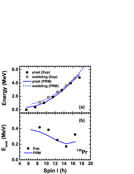
Figure 1: Energy spectra of the yrast (zero-phonon) and wobbling bands (one-phonon) (a) and the corresponding wobbling frequency (b) in ¹³⁵Pr as functions of the total spin $I$ calculated in the PRM in comparison to the experimental data of Ref. Matta et al. (2015).

From the energy spectra, the wobbling frequencies $E_{\rm wob}(I)$ of the theoretical calculation and the data are extracted (as differences) and shown in Fig. 1(b) as a function of spin $I$. In the region $I\leq 14.5\hbar$, both the theoretical and experimental wobbling frequencies decrease with spin, which provides evidence for transverse wobbling motion. At higher spin ($I\geq 14.5\hbar$), the experimental wobbling frequency shows an increasing trend, which indicates that the wobbling mode changes from transverse to longitudinal Matta et al. (2015). The PRM calculations can reproduce this transition well.

In Fig. 2, the separated energy expectation values $E_{\rm{coll}}$ and $E_{\rm{intr}}$ of the collective rotor Hamiltonian $\hat{H}_{\rm{coll}}$ and the intrinsic single-proton Hamiltonian $\hat{H}_{\rm{intr}}$ as calculated in the PRM for the yrast and wobbling bands in ¹³⁵Pr are shown as functions of the spin $I$, together with the differences $\Delta E$ in the two bands and the wobbling frequency.

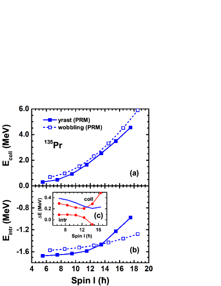
Figure 2: Energy expectation values of the collective rotor (a) and the valence proton (b) calculated in the PRM for the yrast and wobbling bands in ¹³⁵Pr, together with their differences and the full wobbling frequency (c) as functions of the spin $I$.

It is seen that $E_{\rm{coll}}$ increases with the spin, and apparently, the yrast band has lower $E_{\rm{coll}}$ than the wobbling band. The difference of $E_{\rm{coll}}$ in the wobbling and yrast band decreases up to $I=12.5\hbar$, and then it increases rapidly.

In the region $I\leq 11.5\hbar$, the values of $E_{\rm{intr}}$ in the yrast and wobbling bands do not vary much, which implies that the alignment of the proton particle along the $s$-axis remains almost unchanged. This is a specific feature of the wobbling mode in contrast to the cranking mode, where the alignment of the single particle varies with the spin Ødegård et al. (2001); Hamamoto (2002). The values of $E_{\rm{intr}}$ in the yrast band are a bit smaller than those in the wobbling band, but their differences stay almost constant. As a consequence, the decrease of the wobbling frequencies originates mainly from the decrease of the $E_{\rm{coll}}$ differences.

However, from $I=13.5\hbar$ upward, $E_{\rm{intr}}$ of the yrast band increases rapidly, which is caused by the change of alignment of the proton particle from the $s$-axis towards the $i$-axis, driven by the Coriolis interaction. As revealed by the azimuthal plots (discussed later), this corresponds to a change of the rotational mode from along a principal axis ($s$-axis) to a planar rotation (with $\bm{I}$ lying in the $si$-plane). This rearrangement leads to much larger values of $E_{\rm{intr}}$ in the yrast band than in the wobbling band, and hence their difference decreases to negative value for $I\geq 12.5\hbar$.

IV.2 Azimuthal plot

The successful reproduction of the energy spectra in the yrast and wobbling bands for ¹³⁵Pr suggests that the PRM calculation describes well the wave functions underlying the experimental states. Let us now investigate the angular momentum geometry of the system in detail.

In Fig. 3, the obtained profiles $\mathcal{P}(\theta,\varphi)$ for the orientation of the angular momenta $\bm{I}$ in the $\theta\varphi$-plane are shown at spin $I=5.5$, 9.5, 13.5, and $17.5\hbar$ for the yrast band, and at $I=6.5$, 10.5, 14.5, and $18.5\hbar$ for the wobbling band in ¹³⁵Pr. We remind that $\theta$ is the angle between the $\bm{I}$ and the $l$-axis, and $\varphi$ is the angle between the projection of $\bm{I}$ onto the $si$-plane and the $s$-axis.

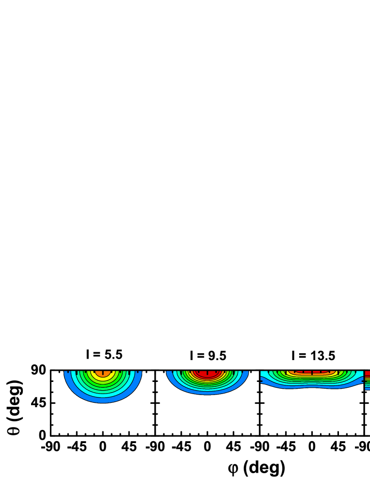
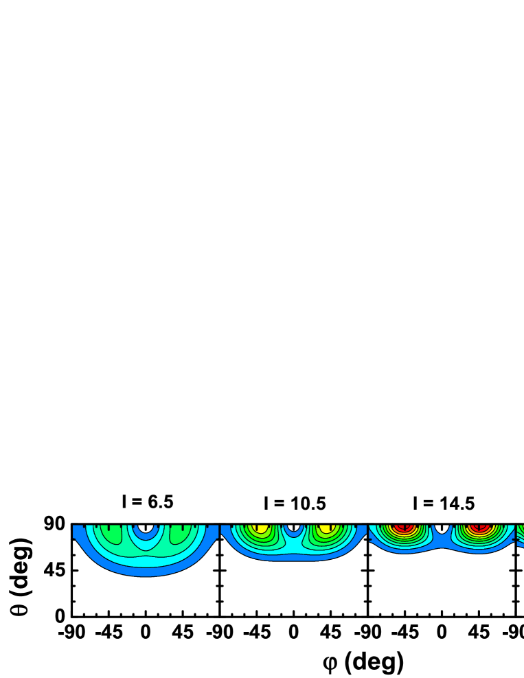
Figure 3: Azimuthal plots (i.e. distributions of the orientation of the angular momentum) calculated at $I=5.5$, 9.5, 13.5, and $17.5\hbar$ for the yrast band and at $I=6.5$, 10.5, 14.5, and $18.5\hbar$ for the wobbling band in ¹³⁵Pr.

One observes that the maximum of $\mathcal{P}(\theta,\varphi)$ is always located at $\theta=90^{\circ}$. This is because the $l$-axis carries the smallest MoI, and in order to lower the energy the angular momentum prefers to lie in the $si$-plane. Note that due to the $\textrm{D}_{2}$ symmetry, $\mathcal{P}(\theta,\varphi)$ is an even function of $\varphi$. For the states in the yrast band, the $\varphi$-coordinates of the maxima gradually deviate from zero with increasing spin. As a result, the number of maxima changes from one to two. This implies that the rotational mode in the yrast band changes from a principal axis rotation at the low spins ($I=5.5$ and $9.5\hbar$) to a planar rotation at high spins ($I=13.5\hbar$). By examining the profiles $\mathcal{P}(\theta,\varphi)$ for all yrast states, we find that $I=13.5\hbar$ is the critical spin at which the rotational mode changes (with $\varphi\simeq\pm 5^{\circ}$ at the maxima). At $I=17.5\hbar$, the $\varphi$-coordinates of the maxima of $\mathcal{P}(\theta,\varphi)$ approaches $\pm 90^{\circ}$. In this case, the rotational mode changes from a planar rotation back to a principal axis rotation about the $i$-axis. These features are similar to the behavior of the minima of the total Routhian surface as a function of the rotational frequency, calculated by TAC in the Refs. Chen et al. (2014, 2016). Both PRM and TAC present the same physics picture: a principal axis rotation about the $s$-axis at low spins, a transition to planar rotation at intermediate spins, and a return to principal axis rotation about the $i$-axis at high spins.

In the lower part of Fig. 3, the distributions $\mathcal{P}(\theta,\varphi)$ exhibit a different behavior in the wobbling band. With one-phonon excitation (wobbling motion), the profiles $\mathcal{P}(\theta,\varphi)$ have two maxima for all spins. At low spins ($I\leq 12.5\hbar$), the excitation is transverse wobbling about the $s$-axis. This is reflected by the larger $\varphi$-values of the maxima of $\mathcal{P}(\theta,\varphi)$ in wobbling states (with spin $I$) compared to those of the corresponding yrast states (with spin $I-1$). Note that for the zero-phonon states (with $I\leq 11.5\hbar$) the underlying wave functions are symmetric and peaked at $\varphi=0^{\circ}$ ($s$-axis), whereas for one-phonon states ($I=6.5\hbar$, $8.5\hbar$, etc.) they are antisymmetric and have a node at $\varphi=0^{\circ}$. At high spins ($I\geq 17.5\hbar$), the excitation from the yrast band into the wobbling band is longitudinal wobbling about the $i$-axis. This is in accordance with the fact that the $\varphi$-coordinate of the maxima of $\mathcal{P}(\theta,\varphi)$ in the wobbling states (with spin $I$) are smaller than those in the yrast states (with spin $I-1$). Moreover, the zero-phonon state ($I=17.5\hbar$) is peaked at $\varphi=\pm 90^{\circ}$ ($i$-axis), while the one-phonon state ($I=18.5\hbar$) has a node there. These features are similar to the properties obtained with wave functions calculated from a collective Hamiltonian in Refs. Chen et al. (2014, 2016).

Therefore, we have confirmed that with the increasing spin, the wobbling mode varies from the transverse at low spins to longitudinal at high spins, which is consistent with the evolution of the wobbling frequency in Fig. 1. In fact, this variation is mainly driven by the collective rotor (cf. Fig. 2).

IV.3 $R$-plots

According to the above analysis, the collective rotor plays an essential role in the wobbling motion. Therefore, we investigate in the following the probability distribution of the rotor angular momentum ($R$-plots) as well as the its projections onto each principal axis ($K_{R}$-plots).

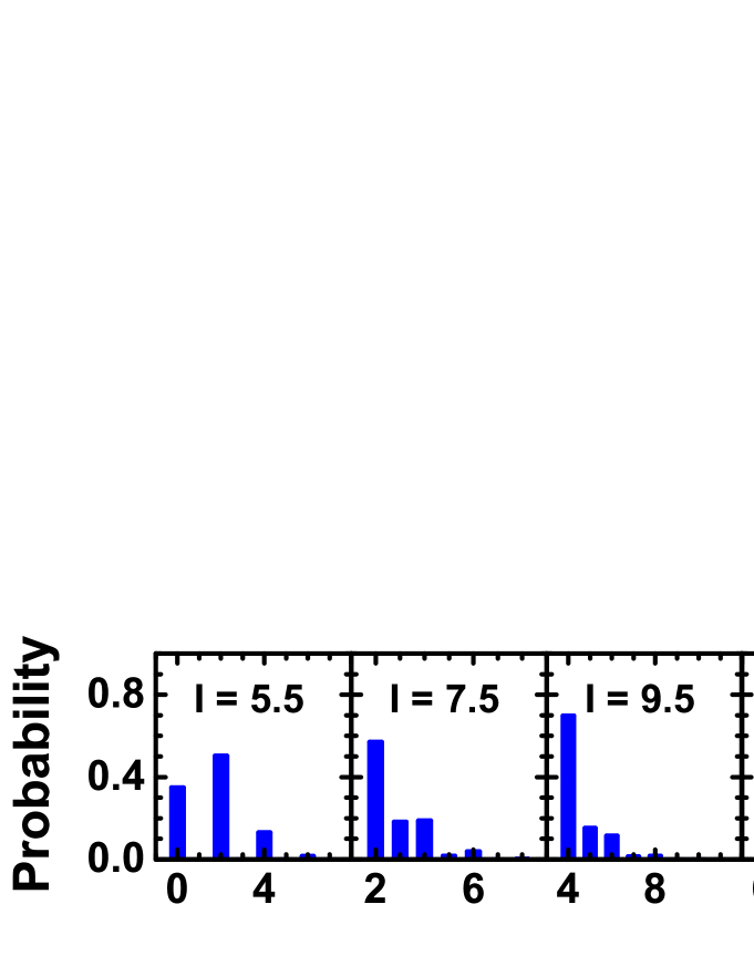
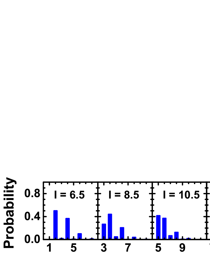
Figure 4: The probability distributions for the angular momentum of rotor ($R$-plots) for the yrast and wobbling bands in ¹³⁵Pr.

In Fig. 4, the probability distributions $P_{R}$ of the rotor angular momentum ($R$-plots) calculated by Eq. (21) are displayed for the yrast and wobbling bands in ¹³⁵Pr. For a given spin $I$, the integer $R$ takes values from $|I-j|$ to $I+j$, excluding $R=1$. It is found that for all $I$ the probability $P_{R}$ almost vanishes for large $R$. Therefore, the $R$-plots are restricted in Fig. 4 to small $R$.

For the yrast band, $P_{R}$ has a pronounced peak at $R_{\textrm{min}}=|I-j|$, except for $I=5.5\hbar$ (the bandhead), where the maximal weight occurs at $R=|I-j|+2=2\hbar$. For the wobbling band, $P_{R}$ has two peaks of similar height, which are located at $R=|I-j|$ and $|I-j|+1$. An exception is again the bandhead $I=6.5\hbar$, where the peaks lie at $R=|I-j|+1$ and $|I-j|+3$. The $R$-plots indicate that $R$ is an asymptotic good quantum number in the yrast band ($I\geq 7.5\hbar$), but not in the wobbling band. This is different to the wobbling motion of a pure triaxial rotor, where $R$ is a good quantum in all bands Bohr and Mottelson (1975); Shi and Chen (2015). However, it should be noted that the admixture of the states with $R=|I-j|$ and $R=|I-j|+1$ in the wobbling band is important as it provides the possibility for the (quantum mechanical) wobbling transition. This admixture causes that the average value of $R$ in the wobbling band $R_{\textrm{wobb}}(I)$ at spin $I$ is larger than $|I-j|$ and leads to $R_{\textrm{wobb}}(I)-R_{\textrm{yrast}}(I-1)>1\hbar$, so that the rotor in the wobbling band with spin $I$ has to wobble to increase its spin by only $1\hbar$ with respect to the yrast band (with spin $I-1$).

IV.4 $K_{R}$-plots

In the following the probability distributions for the projections ($K_{R}=R_{l}$, $R_{s}$, and $R_{i}$) of the rotor angular momentum onto the $l$-, $s$-, and $i$-axes ($K_{R}$-plots) will be investigated. For the triaxiality parameter $\gamma=-26^{\circ}$, the $l$-axis is the designated quantization axis. The distributions with respect to the $s$- and $i$-axis are obtained by taking $\gamma=146^{\circ}$ and $266^{\circ}$, respectively. These $\gamma$-values correspond to the equivalent sectors such that the nuclear shape remains the same, but only the principal axes are interchanged Ring and Schuck (1980).

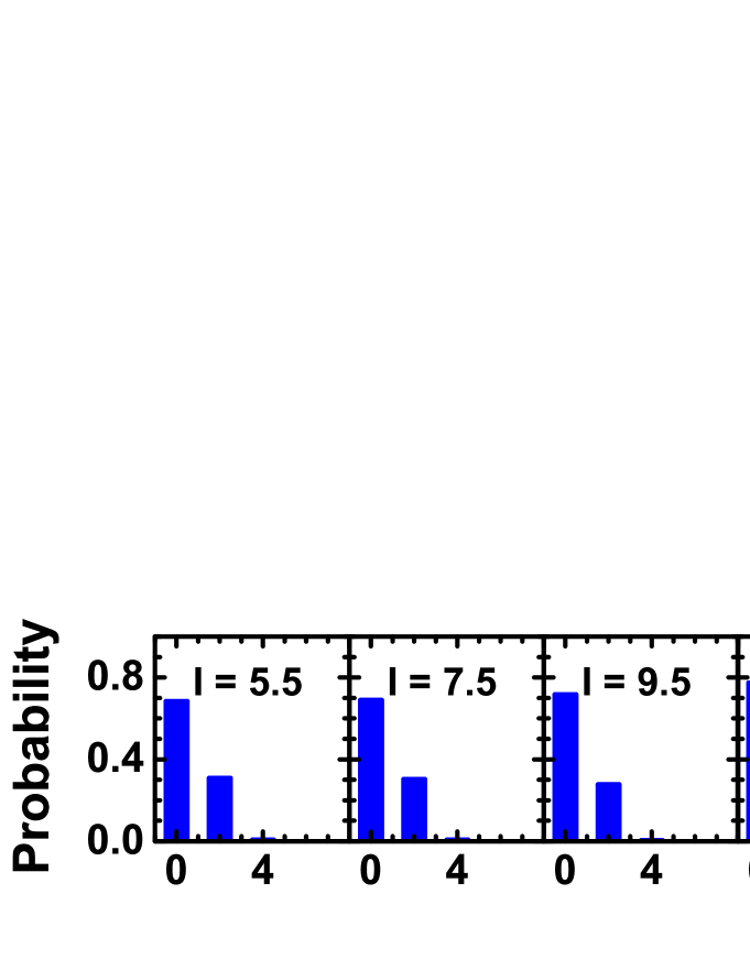
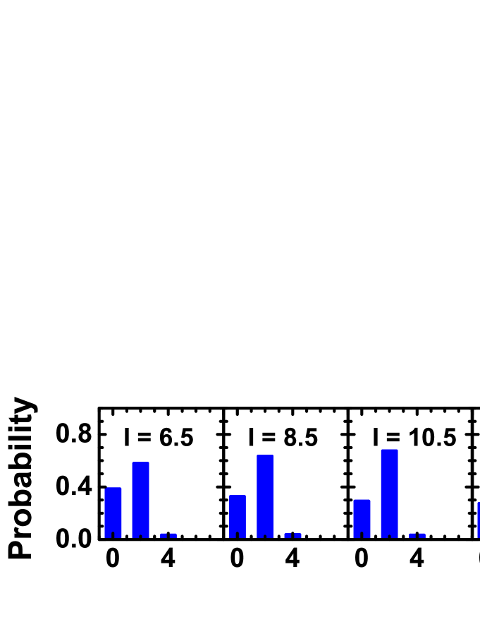
Figure 5: Probability distributions for the projection of the rotor angular momentum onto the $l$-axis for the yrast and wobbling bands in ¹³⁵Pr.

In Fig. 5, the probability distributions for the projection of the rotor angular momentum onto the $l$-axis $P_{R_{l}}$ as calculated in the PRM, are shown for the yrast and wobbling bands in ¹³⁵Pr. For both the yrast and wobbling bands, $P_{R_{l}}$ has two peaks at $R_{l}=0$ and $2\hbar$, indicating that the rotor angular momentum has only very small components along the $l$-axis, to which a very small MoI is associated. This is consistent with the azimuthal plots shown in Fig. 3. At the same time, the distributions of $P_{R_{l}}$ for the yrast and the wobbling bands do not change much as the spin $I$ increases, indicating that the rotor angular momentum component along the $l$-axis remains almost constant. For the yrast band, $P_{R_{l}}$ at $R_{l}=0\hbar$ is much larger than $P_{R_{l}}$ at $R_{l}=2\hbar$, while for the wobbling band, the situation is opposite. There, $P_{R_{l}}$ at $R_{l}=2\hbar$ is larger than $P_{R_{l}}$ at $R_{l}=0\hbar$.

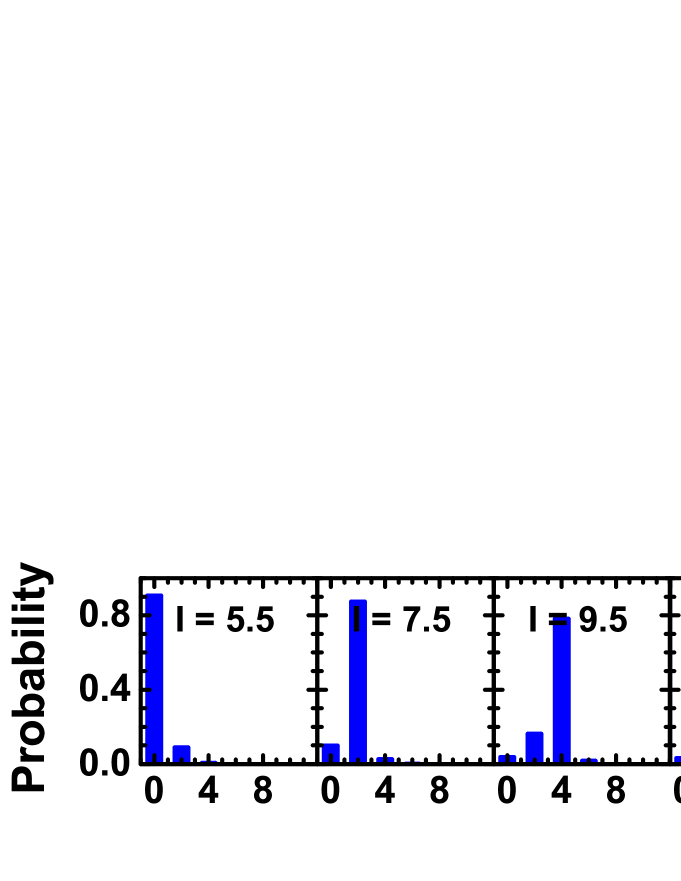
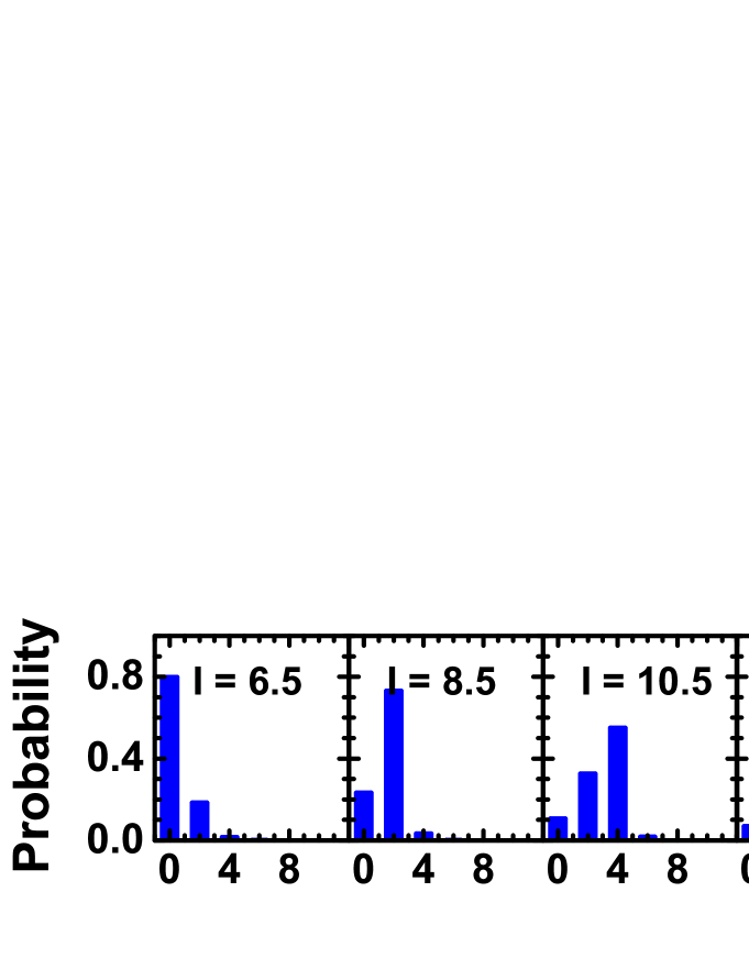
Figure 6: Same as Fig. 5, but for the projection onto the $s$-axis.

The probability distributions $P_{R_{s}}$ of the component $R_{s}$ are displayed in Fig. 6 for the yrast and wobbling bands in ¹³⁵Pr. In the region $I\leq 13.5\hbar$, the distributions $P_{R_{s}}$ for states in the yrast band (with $I-1$) and the wobbling band (with $I$) show a similar behavior. This indicates that the rotor angular momenta of states in the yrast (with $I-1$) and wobbling (with $I$) bands have similar components along the $s$-axis due to the transverse wobbling motion. For neighboring states with $I-2$ and $I$, the distance between the peaks of $P_{R_{s}}$ is $2\hbar$. In the region $I\geq 14.5\hbar$, where the transverse wobbling motion disappears, the distributions $P_{R_{s}}$ are spread over many $R_{s}$-values. The average value of $R_{s}$ is about $4\hbar$ for the yrast band and about $6\hbar$ for the wobbling band.

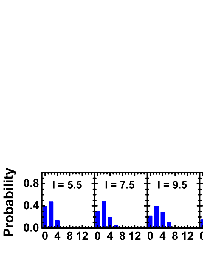
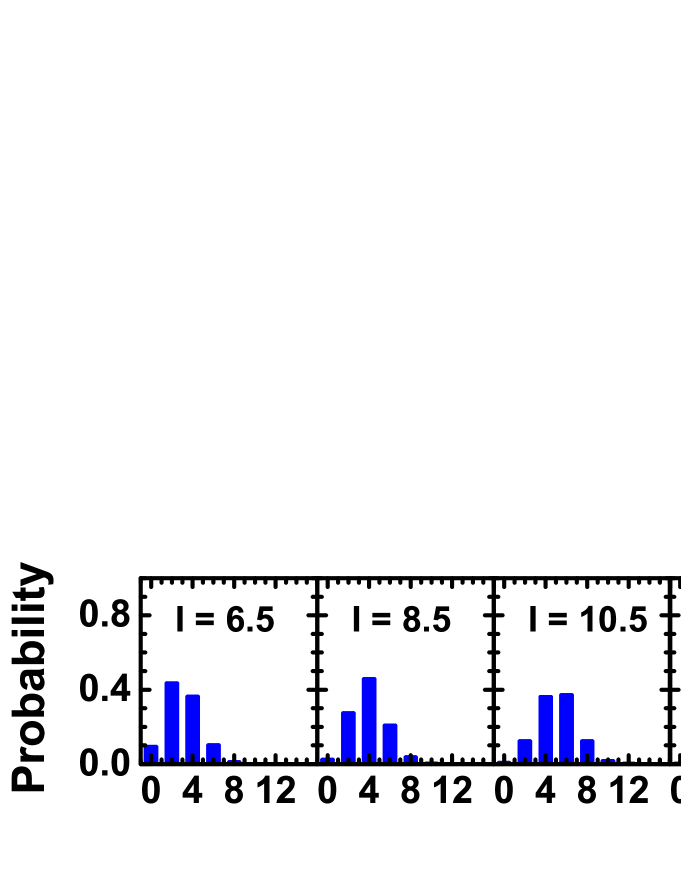
Figure 7: Same as Fig. 5, but for the projection onto the $i$-axis.

In Fig. 7, the probability distributions $P_{R_{i}}$ of the component $R_{i}$ are shown for the yrast and wobbling bands in ¹³⁵Pr. In comparison to $P_{R_{l}}$ and $P_{R_{s}}$, the distributions $P_{R_{i}}$ reveal stronger admixtures of the various values of $R_{i}$, which originates from the wobbling motion of the rotor towards the $i$-axis. One also observes that $P_{R_{i}}$ of the yrast and wobbling bands behavior differently. In the region $I\leq 13.5\hbar$, the probability $P_{R_{i}}$ at $R_{i}=0\hbar$ has a finite value in the yrast band, while it vanishes for the wobbling band. This is a characteristic of the one-phonon excitation of the wobbling motion. Namely, the underlying wave function for a zero-phonon state (yrast band) is even under $R_{i}\to-R_{i}$, whereas for a one-phonon state (wobbling band) it is odd. This picture is also consistent with the features displayed in the azimuthal plots (cf. Fig. 3). The peak position of the distribution $P_{R_{i}}$ increases by about $2\hbar$ from a state in the yrast band (with $I-1$) to a state in the wobbling band (with $I$). This increment is caused by the wobbling motion from the $s$-axis towards the $i$-axis. For neighboring states with $I-2$ and $I$, the average value of $R_{i}$ differs by about $1\hbar$. This means that $R_{i}$ for the state $I$ in the yrast band is about $1\hbar$ smaller than for the state $I-1$ in the wobbling band.

In the region $I\geq 14.5\hbar$, the distributions $P_{R_{i}}$ for the yrast band show a clear peak at $R_{i}=|I-j|=R$ (cf. Figs. 4 and 7), indicating that the rotor has aligned with the $i$-axis. For the wobbling band one observes two peaks of similar height at $R_{i}=|I-j|-1$ and $|I-j|+1$, which gives an increment of $R_{i}$ by about $1\hbar$ from the yrast state (with $I-1$) to the wobbling state (with $I$). This behavior is different from the transverse wobbling region, where the increment is about $2\hbar$.

IV.5 Angular momentum coupling schemes

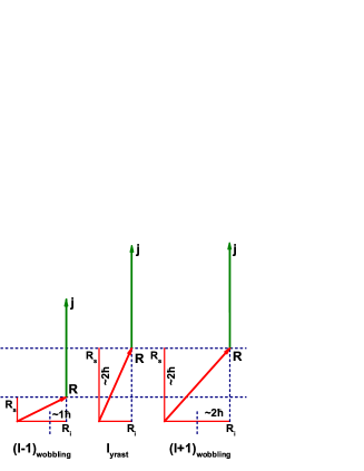
Figure 8: Schematic illustration of the coupling scheme of the angular momenta $\bm{j}$ and $\bm{R}$ of the high-$j$ particle and the rotor for the transverse wobbling in an yrast state with $I$ and two wobbling states with $I\pm 1$. The total angular momentum is $\bm{I}=\bm{R}+\bm{j}$.

From the above analysis of energy expectation values of the intrinsic Hamiltonian $\hat{H}_{\textrm{intr}}$, azimuthal plots $\mathcal{P}(\theta,\varphi)$ of the total angular momentum, and the $R$-plots and three $K_{R}$-plots for the rotor angular momentum, one can deduce the following features in the transverse wobbling region:

• the single-particle (angular momentum) is aligned with the $s$-axis;

• the average rotor angular momentum is more than $1\hbar$ (and less than $2\hbar$) longer in the wobbling band with spin $I+1$ than in the yrast band with spin $I$;

• the projection of the rotor angular momentum onto the $l$-axis is very small;

• the rotor angular momenta in yrast states (with $I$) and wobbling states (with $I+1$) have similar components along the $s$-axis. For neighboring states with $I-2$ and $I$, the component $R_{s}$ differs by about $2\hbar$;

• the component $R_{i}$ increases by about $2\hbar$ from an yrast state $I$ to a wobbling state $I+1$. In addition, $R_{i}$ in the yrast state $I$ is about $1\hbar$ smaller than its value in the wobbling state $I-1$.

Combining these features, a schematic illustration of the coupling scheme of the angular momenta $\bm{j}$ and $\bm{R}$, of the high-$j$ particle and the rotor, for transverse wobbling in an yrast state $I$ and two wobbling states $I\pm 1$ is shown in Fig. 8.

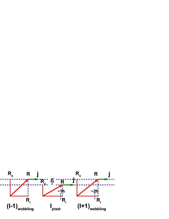
Figure 9: Similar as Fig. 8, but for the longitudinal wobbling motion.

On the other hand, for longitudinal wobbling one finds the following features:

• the proton particle (angular momentum) is aligned with the $i$-axis;

• the average value of $R_{s}$ is about $4\hbar$ in the yrast band and about $6\hbar$ in the wobbling band.

• the increment of $R_{i}$ from an yrast state with $I-1$ to a wobbling state with $I$ is about $1\hbar$.

Again combining these features, a schematic illustration of the coupling scheme of $\bm{j}$ and $\bm{R}$ for the longitudinal wobbling motion in an yrast state with $I$ and two wobbling states with $I\pm 1$ is shown in Fig. 9. This coupling scheme differs from that for transverse wobbling, shown in Fig. 8. One can clearly see that the rotor angular momentum is much longer than the single particle angular momentum. It should be noted that a schematic illustration of the longitudinal wobbling motion has also been given in Refs. Ødegård et al. (2001); Hamamoto (2002), but there the MoI belonging to $s$-axis was assumed to be the largest. In that case, the angular momenta of the rotor and the particle both align with the $s$-axis in the yrast band.

V Summary

In summary, the behavior of the collective rotor for the wobbling motion of ¹³⁵Pr has been investigated in the PRM. After successful reproduction of the experimental energy spectra and the wobbling frequencies, the separate contributions from the rotor and the single-particle Hamiltonian to the wobbling frequencies have been analyzed. It is found that the collective rotor motion is responsible for the decrease of the wobbling frequency in transverse wobbling, and its increase in longitudinal wobbling.

The evolution of the wobbling mode in ¹³⁵Pr from transverse at low spins to longitudinal at high spins has been illustrated by the distributions $\mathcal{P}(\theta,\varphi)$ of the total angular momentum in the intrinsic frame (azimuthal plots). According to the analysis of the probability distributions of the rotor angular momentum ($R$-plots) and their projections onto the three principal axes ($K_{R}$-plots), different schematic coupling schemes of the angular momenta $\bm{j}$ and $\bm{R}$ of the rotor and the high-$j$ particle in the transverse and longitudinal wobbling have been obtained.

In perspective, the $R$-plots and $K_{R}$-plots presented in this work can be used to examine the fingerprints of electromagnetic transitions ($E2$ or $M1$) between wobbling bands, or can be extended to investigate, e.g., the behavior of the collective rotor for chiral rotation Frauendorf and Meng (1997).

References

- Frauendorf and Meng (1997) S. Frauendorf and J. Meng, Nucl. Phys. A 617, 131 (1997).
- Bohr and Mottelson (1975) A. Bohr and B. R. Mottelson, Nuclear structure, vol. II (Benjamin, New York, 1975).
- Frauendorf and Dönau (2014) S. Frauendorf and F. Dönau, Phys. Rev. C 89, 014322 (2014).
- Bringel et al. (2005) P. Bringel, G. B. Hagemann, H. Hübel, A. Al-khatib, P. Bednarczyk, A. Bürger, D. Curien, G. Gangopadhyay, B. Herskind, D. R. Jensen, et al., Eur. Phys. J. A 24, 167 (2005).
- Ødegård et al. (2001) S. W. Ødegård, G. B. Hagemann, D. R. Jensen, M. Bergström, B. Herskind, G. Sletten, S. Törmänen, J. N. Wilson, P. O. Tjøm, I. Hamamoto, et al., Phys. Rev. Lett. 86, 5866 (2001).
- Jensen et al. (2002) D. R. Jensen, G. B. Hagemann, I. Hamamoto, S. W. Ødegård, B. Herskind, G. Sletten, J. N. Wilson, K. Spohr, H. Hübel, P. Bringel, et al., Phys. Rev. Lett. 89, 142503 (2002).
- Schönwaßer et al. (2003) G. Schönwaßer, H. Hübel, G. B. Hagemann, P. Bednarczyk, G. Benzoni, A. Bracco, P. Bringel, R. Chapman, D. Curien, J. Domscheit, et al., Phys. Lett. B 552, 9 (2003).
- Amro et al. (2003) H. Amro, W. C. Ma, G. B. Hagemann, R. M. Diamond, J. Domscheit, P. Fallon, A. Gorgen, B. Herskind, H. Hübel, D. R. Jensen, et al., Phys. Lett. B 553, 197 (2003).
- Hartley et al. (2009) D. J. Hartley, R. V. F. Janssens, L. L. Riedinger, M. A. Riley, A. Aguilar, M. P. Carpenter, C. J. Chiara, P. Chowdhury, I. G. Darby, U. Garg, et al., Phys. Rev. C 80, 041304 (2009).
- Zhu et al. (2009) S. J. Zhu, Y. X. Luo, J. H. Hamilton, A. V. Ramayya, X. L. Che, Z. Jiang, J. K. Hwang, J. L. Wood, M. A. Stoyer, R. Donangelo, et al., Int. J. Mod. Phys. E 18, 1717 (2009).
- Luo et al. (2013) Y. X. Luo, J. H. Hamilton, A. V. Ramayya, J. K. Hwang, S. H. Liu, J. O. Rasmussen, S. Frauendorf, G. M. Ter-Akopian, A. V. Daniel, and Y. T. Oganessian, in Exotic nuclei: Exon-2012: Proceedings of the international symposium (2013).
- Matta et al. (2015) J. T. Matta, U. Garg, W. Li, S. Frauendorf, A. D. Ayangeakaa, D. Patel, K. W. Schlax, R. Palit, S. Saha, J. Sethi, et al., Phys. Rev. Lett. 114, 082501 (2015).
- Biswas et al. (2017) S. Biswas et al., arXiv: nucl-ex, 1608.07840 (2017).
- Sheikh et al. (2016) J. A. Sheikh, G. H. Bhat, W. A. Dar, S. Jehangir, and P. A. Ganai, Phys. Scr. 91, 063015 (2016).
- Chen et al. (2016) Q. B. Chen, S. Q. Zhang, and J. Meng, Phys. Rev. C 94, 054308 (2016).
- Tanabe and Sugawara-Tanabe (2017) K. Tanabe and K. Sugawara-Tanabe, Phys. Rev. C 95, 064315 (2017).
- Budaca (2018) R. Budaca, Phys. Rev. C 97, 024302 (2018).
- Ring and Schuck (1980) P. Ring and P. Schuck, The nuclear many body problem (Springer Verlag, Berlin, 1980).
- Faessler and Toki (1975) A. Faessler and H. Toki, Phys. Lett. B 59, 211 (1975).
- Toki and Faessler (1976) H. Toki and A. Faessler, Phys. Lett. B 63, 121 (1976).
- Smith and Rickey (1976) H. A. Smith and F. A. Rickey, Phys. Rev. C 14, 1946 (1976).
- Ragnarsson and Semmes (1988) I. Ragnarsson and P. B. Semmes, Hyperfine Interactions 43, 425 (1988).
- Mukherjee et al. (1994) A. Mukherjee, U. Datta Pramanik, M. S. Sarkar, and S. Sen, Phys. Rev. C 50, 1868 (1994).
- Modi et al. (2017a) S. Modi, M. Patial, P. Arumugam, E. Maglione, and L. S. Ferreira, Phys. Rev. C 95, 024326 (2017a).
- Dönau and Frauendorf (1977) F. Dönau and S. Frauendorf, Phys. Lett. B 71, 263 (1977).
- Quan et al. (2017) S. Quan, W. P. Liu, Z. P. Li, and M. S. Smith, Phys. Rev. C 96, 054309 (2017).
- Esbensen and Davids (2000) H. Esbensen and C. N. Davids, Phys. Rev. C 63, 014315 (2000).
- Davids and Esbensen (2004) C. N. Davids and H. Esbensen, Phys. Rev. C 69, 034314 (2004).
- Modi et al. (2017b) S. Modi, M. Patial, P. Arumugam, E. Maglione, and L. S. Ferreira, Phys. Rev. C 95, 054323 (2017b).
- Modi et al. (2017c) S. Modi, M. Patial, P. Arumugam, L. S. Ferreira, and E. Maglione, Phys. Rev. C 96, 064308 (2017c).
- Wang et al. (2009) S. Y. Wang, B. Qi, and S. Q. Zhang, Chin. Phys. Lett. 26, 052102 (2009).
- Chen et al. (2017) F. Q. Chen, Q. B. Chen, Y. A. Luo, J. Meng, and S. Q. Zhang, Phys. Rev. C 96, 051303 (2017).
- Chen and Meng (2018) Q. B. Chen and J. Meng, arXiv: nucl-th, 1804.07905 (2018).
- Hamamoto (2002) I. Hamamoto, Phys. Rev. C 65, 044305 (2002).
- Chen et al. (2014) Q. B. Chen, S. Q. Zhang, P. W. Zhao, and J. Meng, Phys. Rev. C 90, 044306 (2014).
- Shi and Chen (2015) W. X. Shi and Q. B. Chen, Chin. Phys. C 39, 054105 (2015).