Chlorine Isotope Ratios in M Giants

Abstract

We have measured the chlorine isotope ratio in six M giant stars using HCl 1-0 P8 features at 3.7 microns with R $\sim$ 50,000 spectra from Phoenix on Gemini South. The average Cl isotope ratio for our sample of stars is 2.66 $\pm$ 0.58 and the range of measured Cl isotope ratios is 1.76 $<$ ³⁵Cl/³⁷Cl $<$ 3.42. The solar system meteoric Cl isotope ratio of 3.13 is consistent with the range seen in the six stars. We suspect the large variations in Cl isotope ratio are intrinsic to the stars in our sample given the uncertainties. Our average isotopic ratio is higher than the value of 1.80 for the solar neighborhood at solar metallicity predicted by galactic chemical evolution models. Finally the stellar isotope ratios in our sample are similar to those measured in the interstellar medium.

1 Introduction

The odd, light elements are useful for understanding the production sites of secondary nucleosynthesis processes. However, some of the odd light elements, such as P, Cl, and K have few measured stellar abundances and/or do not match predicted chemical evolution models (see Nomoto et al. 2013 for a review). For example, chlorine may be made through multiple nucleosynthesis processes but few studies of Cl in the Galaxy exist.

Cl has two stable isotopes. ³⁵Cl is thought to be produced primarily by proton capture on ³⁴S during explosive oxygen burning (³⁴S(p,$\gamma$)), where free protons are created from the ¹⁶O + ¹⁶O reaction or from photodisintigration (Woosley et al., 1973). ³⁷Cl is thought to be produced primarily by the decay of ³⁷Ar (produced via neutron capture on ³⁶Ar) during oxygen burning in core collapse supernova (Woosley et al., 1973; Thielemann & Arnett, 1985; Woosley & Weaver, 1995).

In core collapse supernova (CCSNe), the mass and metallicity of the supernova can impact the isotopic ratio of Cl. Examples of yields from different core CCSNe models are listed in Table 1. The weak s-process in massive stars may also be a significant source of ³⁷Cl. Models predict that ³⁷Cl production increases with He-core mass and neutron excess (Prantzos et al., 1990). For example, in a 25 M_⊙ solar mass star, ³⁷Cl can be over-abundant by a factor of nearly 50 compared to the solar system ³⁷Cl abundance (Pignatari et al., 2010). ³⁷Cl production via the s-process in AGB stars is not thought to be as significant as from the weak s-process (Cristallo et al., 2015; Karakas & Lugaro, 2016). For example, FRUITY models predict only a $\sim$ 3$\%$ increase in ³⁷Cl for a 4 M_⊙ solar metallicity AGB star and a 14$\%$ increase from the initial surface abundance to that after the final dredge up for a 2 M_⊙, solar metallicity AGB star (Cristallo et al., 2015). Also, Karakas & Lugaro (2016) predict a 3 M_⊙ stars with Z = 0.014 and an initial Cl isotope ratio of 3.13, will end with an isotope ratio of $\sim$ 2.6 at the tip of the asymptotic giant branch.

A small amount of chlorine is also predicted to be created during Type Ia supernovae with an isotope ratio between 3 - 5 depending on the model parameters (Travaglio et al., 2004; Leung & Nomoto, 2017). However, Type Ia supernovae yields are not as significant as CCSNe, since the explosive material has little hydrogen available for proton capture (Leung & Nomoto, 2017). For example, the benchmark models of Travaglio et al. (2004) and Kobayashi et al. (2011) demonstrate yields from Type Ia supernovae are an order of magnitude smaller than CCSNe yields, as shown in Table 1. Finally, ³⁵Cl may also be produced from neutrino spallation during CCSNe (Pignatari et al., 2016). A summary of the different yields and production factors from these sources are listed in Table 1.

The chemical evolution model from Kobayashi et al. (2011) predicts Cl isotope ratios in the solar neighborhood of ³⁵Cl/³⁷Cl = 1.94 at [Fe/H] = –0.5 and a Cl isotope ratio of ³⁵Cl/³⁷Cl = 1.80 at solar metallicity. This value is lower than the solar system meteoric Cl abundance of 3.13 (Lodders et al., 2009).

Cl abundance measurements are difficult in stellar spectra due to a low abundance and no strong optical absorption features. ³⁵Cl abundances in stars have been measured using the H³⁵Cl feature located at 3.7 $\mu$m in stars with T $<$ 4000 K (Maas et al., 2016). Stars with temperatures above $\sim$ 4000 K do not have HCl features in their spectra due to the molecule’s low dissociation energy. In the star RZ Ari, both the H³⁵Cl and H³⁷Cl were detected and a Cl isotope ratio of 2.2 $\pm$ 0.4 was derived (Maas et al., 2016). This star is the coolest of their sample with an effective temperature of 3340 K (McDonald et al., 2012).

Table 1: Nucleosynthesis Predictions

Nucleosynthesis Site	Model Parameters	source	Yields 35Cl	Yields 37Cl	Production	Production	35Cl/37Cl
			(M⊙)	(M⊙)	Factor 35Cl	Factor 37Cl
CCSNe	13 M⊙, Z = 0.02, E = 1051 ergs	1	1.15 x 10-4	3.03 x 10-5	$\cdots$	$\cdots$	3.80
CCSNe	13 M⊙, Z = 0.014	2	1.18 x 10-4	2.79 x 10-5	$\cdots$	$\cdots$	4.23
CCSNe	13 M⊙, Z = 0.014, rotation included	2	1.64 x 10-4	4.82 x 10-5	$\cdots$	$\cdots$	3.40
CCSNe	25 M⊙, Z = 0.02, E = 1051 ergs	3	3.63 x 10-4	3.03 x 10-4	$\cdots$	$\cdots$	1.20
CCSNe	25 M⊙, Z = 0.014	2	2.92 x 10-4	1.25 x 10-4	$\cdots$	$\cdots$	2.34
CCSNe	25 M⊙, Z = 0.014, rotation included	2	5.45 x 10-4	1.85 x 10-4	$\cdots$	$\cdots$	2.95
Type Ia SNe	Model b30 3d 768	4	4.58 x 10-5	1.21 x 10-5	$\cdots$	$\cdots$	3.79
AGB Star	3 M⊙, Z = 0.014	5	$\cdots$	$\cdots$	0.90	1.42	2.34
AGB Star	3 M⊙, Z = 0.014	6	$\cdots$	$\cdots$	0.997	1.13	2.60
Weak s-process in He and C Shells	25 M⊙, Z = 0.014	7	$\cdots$	$\cdots$	0.2 - 0.3	46 - 47	$\cdots$

Note. — Sources: (1) Kobayashi et al. 2006; (2) Chieffi & Limongi 2013; (3) Kobayashi et al. 2011; (4) Travaglio et al. 2004; (5) Karakas & Lugaro 2016; (6) Cristallo et al. 2015; (7) Pignatari et al. 2010

The Cl isotopic ratio has been explored in the interstellar medium (ISM) using chlorine bearing molecules in the millimeter/radio regime. Surveys of the Cl isotope ratio have used HCl features and have found a range of isotope ratios in the ISM, from 1 $\lesssim$ ³⁵Cl/³⁷Cl $\lesssim$ 5. HCl in the interstellar medium has been examined using both space based and ground based observatories. Chloronium (H₂Cl⁺) has also been used to probe Cl isotope ratios after the molecule was discovered in the interstellar medium using the Herschel Space Observatory (Lis et al., 2010). Finally, the Cl isotope ratio has been derived in the circumstellar envelopes of evolved stars using NaCl, AlCl, KCl, and HCl. A discussion of ISM ³⁵Cl/³⁷Cl measurements can be found in section 4.2 (see also Table 6).

The range of measured isotope ratios may reflect different nucleosynthesis histories of the material but the systematic errors that may have been introduced in different studies make comparisons difficult. Also, chemical fractionation is not expected to be significant for Cl due to the similar masses of each isotope (Kama et al., 2015). To test predictions of Cl nucleosynthesis, we have measured the Cl isotope ratio in M giants. Observations and data reductions are discussed in section 2. The methodology used to derive Cl isotope ratios is discussed in section 3. A discussion of the results can be found in section 4. We summarize our conclusions in section 5

2 Observations and Data Reduction

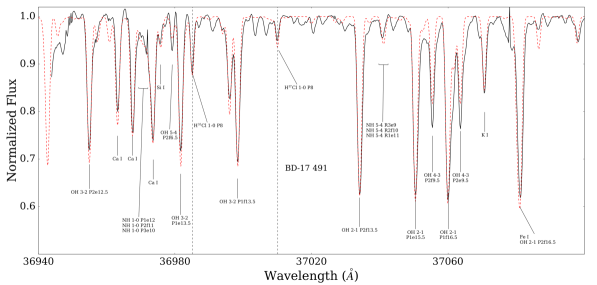
Figure 1: Spectrum of the M-star BD -17 491. The red dashed line represents a model spectrum created to fit the absorption lines for this star. Line identifications are added with the sources for each transition found in section 3.2.

We chose stars from the 2MASS and WISE catalogs (Skrutskie et al., 2006; Wright et al., 2010). Only cool stars are expected to have both the H³⁵Cl and H³⁷Cl features due to the low dissociation energy of the HCl molecule. To ensure our sample of stars contained both HCl features, we calculated the effective temperatures of our stars (as described in section 3.1), and chose stars with photometric temperatures similar to RZ Ari at $\sim$ 3340 K. RZ Ari was the coolest star in the sample of Maas et al. (2016) and the only star in which H³⁷Cl was detected. Stars redder than RZ Ari, with J-K${}_{s}\gtrsim$ 1.26, were initially selected as target stars. We selected stars between 2.0 mags $<$ K${}_{s}<$ 3.0 mags for our sample. These stars were faint enough that they did not saturate the detector in ideal observing conditions. Known binaries stars were found using SIMBAD database and removed from the sample. The full target list, relevant photometry, and spectral types are shown in Table 2. The spectrum of BD –17 491 is shown in Fig. 1 to demonstrate the absorption features in our spectral range.

The observations were obtained at the Gemini South telescope using the Phoenix instrument (Hinkle et al., 1998) for the program GS-2016B-Q-77. The 4 pixel slit was used on Phoenix to achieve a resolution of $\sim$50,000. We used the blocking filter L2734 to observe echelle order 15 covering the wavelength range between 36950 $\AA$ - 37115 $\AA$. Target stars were nodded along the slit and observed in ’abba’ position pairs for sky subtraction during data reduction. Stars were nodded at 3.5” to avoid contamination during sky-subtraction from the broadened profile of the star present during poor seeing conditions. A and B type stars were observed and the airmass differences between the telluric standard observations and target observations were less than 0.1.

Table 2: Summary of Phoenix Observations

2MASS	Other ID	UT Date	J	Ks	W3	Spectral	S/N
Number		Observed	(Mag)	(Mag)	(Mag)	Type
2MASS J00243149-0954040	GN Cet	2016 Dec 15	4.052	2.714	1.826	M6	190
2MASS J00465746-4758522	AH Phe	2016 Dec 8	3.764	2.45	2.146	M6 III	300
2MASS J02323698-1643360	BD-17 491	2016 Dec 8	3.673	2.366	1.844	M5	230
2MASS J04195770-1843196	AV Eri	2016 Dec 11	4.254	2.822	1.683	M6.5	180
2MASS J07042577-0957580	BQ Mon	2016 Dec 10	3.888	2.027	1.278	M7	220
2MASS J07300768-0923169	KO Mon	2016 Dec 15	4.312	2.67	1.566	M6	180

Standard IR data reduction procedures were followed (Joyce, 1992). Data reduction was performed using the IRAF software suite follwing the same procedures as Maas et al. (2016). To summarize, the images were were trimmed, flat-fielded using a dark corrected flat field image, and sky-subtracted. The spectra were extracted, average combined, normalized, and corrected for telluric lines. The wavelength solution was derived using stellar lines in the spectra. The telluric lines were sparse in our spectral range (shown in Fig. 2 in Maas et al. 2016) and provided an inferior wavelength solution than the stellar lines in these M stars.

3 Measuring the Cl Isotope Ratio

First, equivalent widths of the two HCl features at 36985 $\AA$ (H³⁵Cl) and 37010 $\AA$ (H³⁷Cl) were measured using the deblending tool in splot. Both HCl lines have nearly identical excitation potentials and log gf values (Rothman et al., 2013), which are listed in Maas et al. (2016). The chlorine isotope ratio was found in RZ Ari by taking the ratio of the equivalent widths of the H³⁵Cl line and the H³⁷Cl line (Maas et al., 2016). Both HCl features in that star had weak line strengths on the linear portion of the curve of growth. We compared our 6 stars to curve of growth models for the two HCl lines and found small deviations from the linear approximation. The curves of growth were created using MOOG (Sneden 1973, v. 2014) and MARCS model atmospheres (Gustafsson et al., 2008). The full line list used to create the model spectrum in Fig. 1 is listed in Maas et al. (2016).

3.1 Atmospheric Parameters

Atmospheric parameters are needed to determine the position of the HCl features on the curve of growth (COG). The effective temperature and microturbulence most impacted the shape of the COG when generating models. Spectral types for our stars were determined from the SIMBAD database and are listed in Table 2, however, no stars have atmospheric parameters derived in the literature. We first determined that our stars are giants from two arguments. The J-K_s colors for the stars are consistent with giants: for example the intrinsic J-K_s for an M5 giant is 1.36 while a dwarf M5 star has 0.77 (Jian et al., 2017). Additionally, the Ca I lines observed between 36960 - 36975 $\AA$ are broadened at higher gravities. The Ca I lines for the stars in our sample are similar to BD –17 491, shown in Fig. 1, and are consistent with the spectra of giants.

Temperatures were derived using the J-W3 color with J-band photometry from 2MASS (Skrutskie et al., 2006) and the the W3 band from WISE (Wright et al., 2010). The temperature-color relation from Jian et al. (2017) was used and the temperature derived for each star is listed in Table 3. This temperature-color relation is calibrated for giants between 3650 K $<$ T_eff $<$ 5100 K and so the relation was extrapolated to determine the temperatures for our stars. The spectral energy distribution was constructed for each star using photometry from 2MASS (Skrutskie et al., 2006), WISE (Wright et al., 2010), and IRAS (Beichman et al., 1988). The Rayleigh-Jeans tail of the spectral energy distribution (SED) was compared to a blackbody function to determine if any of the sample stars show a significant infrared excess. For each star, a single scaled blackbody function fits the infrared portion of the curve except for deviations at $\sim$ 100 $\mu$m.

The J and W3 bands were used due to the uncertainty on the K_s, W1, and W2 photometric measurements. The W1 and W2 Wise bands were saturated and the average W3 band uncertainty is 0.02 $\pm$ 0.007 mags. The average J-band magnitude error is 0.27 $\pm$ 0.03 for the sample and the $K_{s}$ magnitudes had uncertainties similar to the J band magnitudes. The cores of the star images are saturated in the 2MASS photometry and the large photometric error was estimated from the fit to the unsaturated portion of the 1-D radial profile fit (Skrutskie et al., 2006). A J magnitude range of $\pm$ 0.27 mags translates into a temperature difference of $\sim$ 150 K for the stars in our sample. Due to the uncertainty on the J band magnitude and the extrapolation of the temperature-color relation, an uncertainty of $\pm$ 200 K is appropriate for our derived temperatures.

The microturbulence values ($\xi$) were derived by fitting COG models to the OH lines in our spectral range. OH line equivalent widths were measured using the deblending tool within splot in IRAF. The equivalent width values are listed in Table 4. Uncertainties were estimated by measuring the equivalent width multiple times at different continuum levels. Empirical curves of growth were created for each star with a range of microturbulence values in steps of 0.1 km/s. The models were created at the temperature of the star, log g = 0.5, and at solar metallicity. COGs were created using MOOG and OH excitation potential and log gf values from Brooke et al. (2016). The log gf values were tested by fitting the spectra of Arcturus and the Sun (Maas et al., 2016).

Table 3: Atmospheric Parameters and Cl Isotope Ratios

Star Name	Temperature	$\xi$	H35Cl EW	H37Cl EW	35Cl/37Cl
	(K)	(km/s)	(m$\AA$)	(m$\AA$)
GN Cet	3102	2.5 $\pm$ 0.2	165 $\pm$ 10	106 $\pm$ 8	1.76 $\pm$ 0.17
AH Phe	3516	2.5 $\pm$ 0.2	122 $\pm$ 11	63 $\pm$ 8	2.20 $\pm$ 0.30
BD -17 491	3355	2.3 $\pm$ 0.2	137 $\pm$ 9	66 $\pm$ 8	2.42 $\pm$ 0.30
AV Eri	2921	1.4 $\pm$ 0.3	161 $\pm$ 12	62 $\pm$ 8	3.42 $\pm$ 0.50
BQ Mon	2902	1.6 $\pm$ 0.2	185 $\pm$ 11	81 $\pm$ 6	2.92 $\pm$ 0.31
KO Mon	2838	2.4 $\pm$ 0.2	243 $\pm$ 19	98 $\pm$ 9	3.22 $\pm$ 0.42
RZ Ari	3340	2.54 $\pm$ 0.15	81 $\pm$ 6	36 $\pm$ 6	2.2 $\pm$ 0.4

Table 4: OH Equivalent Width Measurements

Wavelength	GN Cet	AH Phe	BD -17 491	AV Eri	BQ Mon	KO Mon
($\AA$)	EW (m$\AA$)	EW (m$\AA$)	EW (m$\AA$)	EW (m$\AA$)	EW (m$\AA$)	EW (m$\AA$)
36954.896	440 $\pm$ 30	468 $\pm$ 23	450 $\pm$ 32	441 $\pm$ 26	476 $\pm$ 43	502 $\pm$ 38
36979.19	74 $\pm$ 15	94 $\pm$ 20	81 $\pm$ 18	113 $\pm$ 18	120 $\pm$ 27	85 $\pm$ 15
36981.688	420 $\pm$ 21	438 $\pm$ 29	417 $\pm$ 19	399 $\pm$ 27	465 $\pm$ 31	422 $\pm$ 23
36998.379	527 $\pm$ 14	489 $\pm$ 27	491 $\pm$ 33	441 $\pm$ 33	491 $\pm$ 32	513 $\pm$ 28
37034.102	624 $\pm$ 46	675 $\pm$ 33	618 $\pm$ 27	575 $\pm$ 33	637 $\pm$ 34	674 $\pm$ 43
37050.462	655 $\pm$ 39	662 $\pm$ 28	642 $\pm$ 53	601 $\pm$ 24	628 $\pm$ 44	730 $\pm$ 45
37055.419	381 $\pm$ 40	338 $\pm$ 42	334 $\pm$ 51	316 $\pm$ 33	318 $\pm$ 40	356 $\pm$ 42
37059.961	724 $\pm$ 36	643 $\pm$ 55	599 $\pm$ 18	648 $\pm$ 34	637 $\pm$ 47	835 $\pm$ 48
37063.634	382 $\pm$ 37	384 $\pm$ 17	346 $\pm$ 25	309 $\pm$ 52	353 $\pm$ 14	392 $\pm$ 40

Each empirical COG was shifted until the weak 36979 $\AA$ OH line fell on the model COG when fitting the data; this OH line approximately falls on the linear portion of the COG. Multiple models with different microturublence values, in steps of 0.1 km s^-1 were fit to the data. The model that resulted in the lowest $\chi^{2}$ was chosen as the best value. A Monte-Carlo simulation was performed to determine the error on the derived microturbulence using this method. The OH equivalent widths for each line were adjusted randomly for each iteration from a Gaussian distribution with a mean of the measured value for a line and a standard deviation of the measurement error. The process was repeated for 10,000 iterations and the uncertainty on the microturbulence was set at the 5 $\%$ and 95 $\%$ median values due to the large step sizes in microturbulence. The best fits for the six stars in the sample are shown in Figure 2. We also compared the dependence of the derived temperature on microturbulence. No strong correlation between effective temperature and microturbulence was seen for our sample of stars, as shown in Fig. 3.

To test our method, we determined the microturbulence of RZ Ari since this star has an T_eff of 3340 K, similar to our sample of M giants. The observations for this star are detailed in Maas et al. (2016). The microturbulence from measurements of the OH lines lead to value of $\xi$ = 2.1${}^{+0.3}_{-0.2}$ km s^-1. Our microturbulence measurement is compatible within the uncertainties with the microturbulence from Tsuji (2008), listed in Table 3, and derived from weak molecular lines.

Our derived microturbulence values are also consistent with values found in other evolved M stars. Microturbulences varied between 1.5 - 2.6 km s^-1 for carbon stars in the sample of Lambert et al. (1986). Also, Lambert et al. (1986) noted that stars with the lowest microturbulence values, between 1.5 - 1.8 km s^-1 have anomalous features in their spectra, such as a Mira variable (R Lep), wavelength dependent CO lines abundances (R Scl), and strong CO lines with low abundances (V Hya). Without spectra covering larger wavelength ranges we cannot determine if these anomalies are present in the stars we observed with low microturbulence values. Other studies find microturbulence values for red giants between 2.1 - 3.2 km s^-1 (Cunha et al., 2007).

Surface gravity was assumed to be log g = 0.5; varying the parameter by $\pm$ 0.5 created negligible corrections on the equivalent width, similar to the results of Maas et al. (2016). We also assumed stars in our sample to have solar metallicities. Metal-poor stars with ([Fe/H] $\lesssim$ –1) likely could not reach the low effective temperatures found in our sample.

3.2 Spectral Synthesis

To ensure blends with weak CN/CH lines did not affect the M giants in our sample, we fit synthetic spectra to the stars. The line-list was replicated from Maas et al. (2016), which included OH lines from Brooke et al. (2016), CN line features from Brooke et al. (2014) and accessed via the Kurucz database, NH lines from Brooke et al. (2014, 2015), CH lines from Masseron et al. (2014), and HCl line information from Rothman et al. (2013). The synthetic spectra were generated using pymoogi, a python wrapper that runs MOOG v. 2014 (Sneden, 1973). A plot of the synthetic spectrum for the M star BD –17 491 is shown in Figure 1. Atmospheric parameters for BD –17 491 are described in Section 3.1 with the temperatures and microturbulent velocities listed in Table 3. The abundances were adjusted to provide the best fit to the spectrum for line identification. We find that in stars with C/O $<$ 1, OH lines dominate and CH/CN are weak or negligible. We therefore can measure HCl equivalent widths without blends in spectral type M stars in our sample.

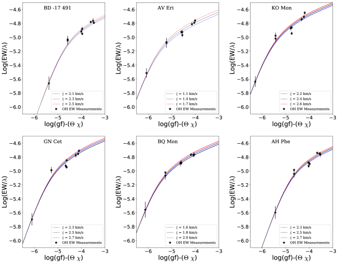
Figure 2: An empirical curve of growth for the OH lines measured for our sample. The x-axis is the log(gf) - ($\Theta$ $\chi$ ): where $\Theta$=5040/T(K) and $\chi$ is the excitation potential. The y-axis represents the reduced equivalent width. Three model curve of growths were created for three different microturbulence values ($\xi$). These models are fit to the measured reduced equivalent widths to determine the microturbulence for the star.

3.3 Cl Isotope Ratios

Model COGs for HCl were created using the effective temperatures and microturbulence values listed in Table 3, an assumed log g value of 0.5, and solar metallicities. The Cl isotope ratio derived from the ratio of equivalent width was adjusted by the distance between the linear approximation and the model curve of growth. Without the correction factor, larger equivalent widths would incorrectly represent smaller abundance. The corrections are most pronounced for the H³⁵Cl line due to its larger line strength. The final chlorine isotope ratio was calculated by taking a ratio of the equivalent widths with corrections for deviations from non-linearity. The results can be found in Table 3.

The dependence of the Cl isotope ratios on photometric effective temperature and microturbulence is explored in Figure 3. From inspection there appears no strong relationship between the microturbulence and isotopic abundance. We estimated the slope between the Cl isotope ratio and effective temperature with a Monte Carlo simulation. Simulated isotope ratios and temperatures were generated as a random Gaussian number with the measured ratio as the mean value and the uncertainty as the standard deviation. A linear fit was done for each set of measured isotopic abundances for 10,000 iterations. The final result was an average slope of –0.1 $\pm$ 4.0 (ratio / 100K). A systematic uncertainty underlying a relationship between T_eff and Cl isotope ratio would induce artificial scatter in the data. However, we note the warmest stars have the weakest HCl lines and therefore the smallest corrections. The Cl isotope ratio measured in these stars are likely the least impacted by any existing systematic effects. The Cl isotope ratio for AH Phe for example is 2.2 $\pm$ 0.3 which still is above the predicted chemical evolution model and is $\sim$ 3$\sigma$ from the solar value. We do not find a significant slope between temperature and abundance given our uncertainties. More accurate effective temperatures and a larger sample are necessary to determine if any relationship exists between effective temperature and Cl isotope ratio.

We used the abfind driver in MOOG to estimate the abundance of ³⁵Cl and ³⁷Cl from the equivalent width measurements. The isotope ratios derived from the abundances agree with the COG method however, the uncertainties on the abundances were significantly larger. We tested the star BD –17 491 and calculated the A(³⁵Cl) and A(³⁷Cl) abundance for the best model parameters, for $\delta$T = $\pm$ 200 K, $\delta$log g = $\pm$ 0.5, [Fe/H] at -1 and 0.5, $\delta\xi$ $\pm$ 0.2 km s^-1, and for the one sigma uncertainties on the equivalent width measurement. The abundances were derived independently and the average difference between the high and low atmospheric parameter were taken as the uncertainty. Each term was added in quadrature to determine the total uncertainty. For BD –17 491, we determined A(³⁵Cl) = 5.00 $\pm$ 0.96 dex and A(³⁷Cl) = 4.61 $\pm$ 1.06 dex. The metallicity and temperature were the main sources of uncertainties, similar to the findings of Maas et al. (2016). Cl abundances were not determined for the rest of our sample because of the large uncertainties. However, the isotope ratio between the two abundances is accurate since errors in the atmospheric parameters will affect both the H³⁵Cl and H³⁷Cl lines equally. The systematic errors will be removed except for uncertainties on the shape of the curve of growth given in Table 5.

3.4 Uncertainties

Uncertainties were estimated for both the atmospheric parameters chosen and the equivalent width measurements. Atmospheric models were created at the 1$\sigma$ level for the stars effective temperature and microturbulence. Additional models were created at a log g of one, a log g of zero, at an [Fe/H] at –1 and 0.5 dex. The uncertainty on the COG nonlinear correction was computed for each atmospheric parameter independently. The uncertainty from each atmospheric parameter and the fit were added in quadrature to determine the final uncertainties on the H³⁵Cl and H³⁷Cl corrected equivalent width measurements. The dominant term is the uncertainty on the H³⁷Cl equivalent width. For example, the uncertainty on the isotope ratio for GN Cet is lower because the H³⁷Cl features is relatively strong. The average uncertainties on the equivalent width corrections are shown in Table 5.

Table 5: Average Uncertainty on Non-Linearity Correction from Atmospheric Parameters

Parameter	H35Cl	H35Cl
	(m$\AA$)	(m$\AA$)
Teff	11	2
log g	4	1
$[Fe/H]$	5	1
$\xi$	7	1

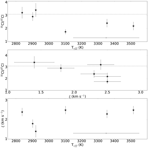
Figure 3: Three plots showing the relationship between the derived atmospheric parameters, effective temperature and microturbulence and the measured Cl isotope abundances in our sample of stars. The top plot shows isotope ratios versus temperature, the middle plot shows isotope ratios versus microturbulence, and finally the bottom plot shows microturbulence versus temperature. The uncertainty on the temperature is estimated to be 200 K for each of our stars, shown by the error bar in the top and bottom plots.

4 Discussion

4.1 Chlorine Isotopologue Nucleosynthesis

Our Cl isotope ratio measurements allow us to explore multiple important questions about the nucleosynethsis of Cl. First, is the Cl isotope ratio in the solar system consistent with our observed isotopic abundances? The meteoric solar Cl isotope ratio falls within the range of measurements in our sample, from 1.76 - 3.42, although it is at the high end.

Next, does our sample agree with the predicted Cl isotope ratio for the solar neighborhood? The chemical evolution model of Kobayashi et al. (2011) predicts Cl isotope ratios in the solar neighborhood of ³⁵Cl/³⁷Cl = 1.94 at an [Fe/H] of –0.5 and a Cl isotope ratio of ³⁵Cl/³⁷Cl = 1.80 at solar metallicity. Our average Cl isotope ratio is $\sim$ 1.5$\sigma$ higher than this value and AH Phe, BQ Mon, and KO Mon in particular deviate by 2$\sigma$ - 3$\sigma$ from the model prediction for solar metallicity stars. The model prediction is also smaller than the solar system meteoric Cl isotope ratio of 3.13 (Lodders et al., 2009). The offset may be due to either underproduction of ³⁵Cl, or an overproduction of ³⁷Cl in the models. Yields from supernova models that include rotation have larger ³⁵Cl/³⁷Cl ratios for the 25 M_⊙ progenitors (Chieffi & Limongi, 2013) and may help explain the discrepancy between chemical evolution models and measurements. Inclusion of the $\nu$ process, which produces ³⁵Cl may also impact yields from supernovae. Maas et al. (2016) suggests that ³⁵Cl abundances are larger than expected from chemical evolution model of Kobayashi et al. (2011).

Next, is the spread of Cl isotope ratios observed consistent with the measurement errors? The mean isotope ratio and standard deviation of our sample is 2.66 $\pm$ 0.58. Since the measurement precision varied from star to star, we also calculated a weighted mean of ³⁵Cl/³⁷Cl = 2.27 $\pm$ 0.11.

We performed a Monte Carlo simulation to determine if the standard deviation from our six stars is consistent with scatter around a common average Cl isotope ratio or if the scatter in our data reflects differences in the surface composition of our stars. Six random numbers were generated using a Gaussian distribution with a mean equal to the weighted average of our sample and standard deviations derived for our sample stars. The standard deviation was measured for the six values. We continued measuring standard deviations for 50,000 sets of measurements and found that 98.8 $\%$ of the trials had standard deviations less than 0.58. The mean Cl isotope ratio standard deviation from the simulation was 0.30. The observed large standard deviation implies that some portion of the scatter in the Cl isotopic ratio seen in our sample reflects differences in surface abundance and the chemical history of the stars.

The Gaia DR 1 did not include extremely blue or red stars which may be why no parallax measurements are available for our sample (Gaia Collaboration et al., 2016). Additionally, all stars but BD –17 491 are identified as long period variables in the SIMBAD database. AH Phe is the only star classified as luminosity class III and we estimate the distance to this star based on this classification. First, we estimate a luminosity of log(L/L_⊙) = 3.1 for a 1.5 $M_{\odot}$, Z = 0.017 star at T_eff $\sim$ 3500 using stellar evolutionary tracks from Bertelli et al. (2008, 2009). We use the K_s measurement from Table 2 and a bolemetric correction of 3 from Bessell et al. (1998) to determine the distance modulus. We used the color transformation relations of Johnson et al. (2005) to convert the K_s measurements to the Johnson K system. We estimate a distance of $\sim$ 520 pc to AH Phe.

Table 6: Cl Isotope Ratios Measured in the ISM and Stars

Object	Object Type	Cl Ratio	Feature	Reference
IRC+10216	Carbon Star	2.3 $\pm$ 0.5	NaCl, AlCl	(1)
IRC+10216	Carbon Star	3.1 $\pm$ 0.6	NaCl, AlCl, KCl	(2)
IRC+10216	Carbon Star	2.3 $\pm$ 0.24	NaCl, AlCl	(3)
IRC+10216	Carbon Star	3.3 $\pm$ 0.3	HCl	(4)
CRL 2688	Post-AGB (Pre-PN) Star	2.1 $\pm$ 0.8	NaCl	(5)
Orion A	Giant Molecular Cloud (OMC-1)	$\sim$ 4 - 6	HCl	(6)
Multiple Objects	Multiple Objects	1 - 5	HCl	(7)
NGC6334I	Molecular Gas in Embedded Star Cluster/SFR	2.7	H2Cl+	(8)
Sgr A, W31C	Foreground Molecular Clouds towards SgrA, W31C	$\sim$ 2-4	H2Cl+	(9)
PKS 1830-211	Foreground Absorbed towards Lensed Blazar	3.1${}^{+0.3}_{-0.2}$	H2Cl+	(10)
W49N	Diffuse Foreground Absorbers towards H II Region W49N	3.50${}^{+0.21}_{-0.62}$	H2Cl+	(11)
W3	Molecular Cloud toward HII region W3	2.1 $\pm$ 0.5	HCl	(12)
CRL 2136	Molecular Cloud associated with SFR CRL 2136	2.3 $\pm$ 0.4	HCl	(13)
W31C	Absorber towards SFR W31C	2.9	HCl	(14)
OMC-2-FIR-4	Proto-Stellar Core in Orion Nebula	3.2 $\pm$ 0.1	HCl	(15)
W31C	Absorber towards SFR W31C	2.1 $\pm$ 1.5	HCl+	(16)
RZ Ari	Red Giant Star	2.2 $\pm$ 0.4	HCl	(17)
Multiple Stars	Red Giant Stars	1.76 - 3.42	HCl	This Work

Note. — References: (1) Cernicharo & Guelin 1987; (2) Cernicharo et al. 2000; (3) Kahane et al. 2000; (4) Agúndez et al. 2011; (5) Highberger et al. 2003; (6) Salez et al. 1996; (7) Peng et al. 2010; (8) Lis et al. 2010; (9) Neufeld et al. 2012; (10) Muller et al. 2014; (11) Neufeld et al. 2015; (12) Cernicharo et al. 2010; (13) Goto et al. 2013; (14) Monje et al. 2013 ;(15) Kama et al. 2015; (16) De Luca et al. 2012 ;(17) Maas et al. 2016

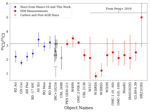
Figure 4: Cl isotope ratios from Table 6 plotted as a function of object name and Cl isotope ratio. The dashed line represents the solar system meteoric Cl isotope ratio. Blue star represent Cl isotope ratios measured in M giants, red octogons are ISM measurements, and black crosses are measurements in the circustellar envelopes of carbon stars and post-AGB stars.

4.2 Comparisons to Cl Isotope Ratios in ISM

We compare our measurements of ³⁵Cl/³⁷Cl to those made in star forming regions, molecular clouds, and the circumstellar envelopes of evolved stars, summarized in Table 6. We find the Cl isotope ratios in stars are consistent with the range measured in the ISM; results from both studies with uncertainties are displayed in Figure 4. The measurements in the ISM are consistent with the solar system value, noted by Muller et al. (2014); Neufeld et al. (2015), including a ³⁵Cl/³⁷Cl = 3.1${}^{+0.3}_{-0.2}$ measurement at a redshift of 0.89 (Muller et al., 2014). Finally, the HCl survey of Peng et al. (2010) found a range of Cl isotopic ratios between 1-5. We find a smaller range between 1.76 $\leq$ ³⁵Cl/³⁷Cl $\leq$ 3.42 of Cl isotope in stars.

Local explosive nucleosynthesis events may partially explain the spread in isotope ratios both in the ISM (Salez et al., 1996; Peng et al., 2010) and in our sample of stars. Studies of dust grains from the winds of evolved stars suggests the disk of the Galaxy well mixed and placed an upper limit on the spread of Si and Ti isotopes due to heterogeneous mixing in the disk at 40$\%$ (Nittler, 2005). A Monte Carlo simulation found the spread in [Fe/H] from heterogeneous mixing was expected to be between 0.022 to 0.03 dex depending on the yields adopted (Nittler, 2005). Assuming solar metallicity, these variations correspond to 5$\%$ - 7$\%$ variations in the ISM. For our average Cl isotope ratio of 2.66, 7$\%$ variations corresponds to a range of 0.19. The Monte Carlo simulation performed in section 4.1 found an expected mean expected standard deviation of 0.30 dex, therefore the heterogeneous mixing in the ISM may explain some of the scatter in our data beyond the measurement uncertainties. Metallicity variations may also play a role in the dispersion seen in the ISM and in our sample of stars. The chemical evolution model of Kobayashi et al. (2011) predicts at [Fe/H] = 0, a ³⁵Cl/³⁷Cl = 1.80, at an [Fe/H] = –0.5 a ³⁵Cl/³⁷Cl = 1.94, and finally the prediction at [Fe/H] = –1.1 is ³⁵Cl/³⁷Cl = 2.62.

Core collapse supernova are thought to be the dominant source of chlorine production and the isotope ratio varies depending on the progenitor star mass, metallicity, and explosion energy. For example, the larger the progenitor star at high metallicity, the lower the lower the Cl isotope ratio, as shown in Table 1. Low mass progenitors may help explain observations of high isotope ratios (e.g. AV Eri with ³⁵Cl/³⁷Cl = 3.42 $\pm$ 0.50) and visa-versa. Also, a 25 M_⊙, Z = 0.02 supernova with an explosion energy of E = 10⁵¹ erg yields a Cl ratio of ³⁵Cl/³⁷Cl $\sim$ 1.2, the same model parameters with E = 10⁵² erg produces an isotope ratio of ³⁵Cl/³⁷Cl = 1.75 (Kobayashi et al., 2011). The Cl isotope ratio from supernova typically increases as the metallicity of the progenitor star decreases. For example, a 25 $M_{\odot}$, Z = 0.004 supernova would have yields of ³⁵Cl/³⁷Cl = 1.75 (Kobayashi et al., 2006), compared to a yield a ratio of 1.2 for a Z = 0.02 (see Table 1).

Studies of the circumstellar material around stars suggested the s-process is creating ³⁷Cl in AGB stars and reducing the Cl isotope ratio. Low Cl isotope ratios were measured in the circumstellar envelopes of IRC+10216 (Kahane et al., 2000) and CRL 2688 (Highberger et al., 2003) (listed in Table 6). Both papers suggested s-process element enhancement in the stars may have caused Cl isotope ratios below the solar system values. However, other studies have found Cl isotope ratios consistent with the solar system value in IRC+10216 and the errors are significant for Cl 2688. Additionally, models only predict modest enhancement of ³⁷Cl in AGB stars (Cristallo et al., 2015; Karakas & Lugaro, 2016). Additionally, our sample of stars were classified through analysis of low resolution spectroscopy and did not show signs of s-process enhancement indicative of an S star (Hansen & Blanco, 1975; Houk, 1978; Kwok et al., 1997).

5 Summary

We measured Cl isotope ratios in six M giants using spectra obtained from Phoenix on Gemini South. Measurements of Cl isotope ratios were performed using effective temperatures derived from J - W3 color and microturbulences from OH equivalent widths and curve of growth models. Cl isotope ratios were found by comparing equivalent widths from HCl 1-0 P8 features. Non-linearity corrections between the equivalent width and abundance were made using curve of growth models. From our Cl isotope ratios we have derived the following results:

1. We find an average Cl isotope ratio and standard deviation of 2.66 $\pm$ 0.58 for our sample of stars. A Monte Carlo simulation suggests the scatter in our measurements reflects differences in surface abundances with over 2$\sigma$ confidence.

2. We find a range of Cl isotope ratios between 1.76 and 3.42 in our sample of stars. The solar system isotope ratio of 3.13 (Lodders et al., 2009) is consistent with this range of measurements.

3. Our average Cl isotope ratio is higher than the predicted value of 1.80 for the solar neighborhood at solar metallicity (Kobayashi et al., 2011)

4. The Cl isotope ratios measured in our sample of stars are consistent with those found in the ISM. The range in Cl isotope ratios may partially be due to different nucleosynthesis events enriching different portions of the ISM and from metallicity variations.

6 Acknowledgements

This work is based on observations obtained at the Gemini Observatory, which is operated by the Association of Universities for Research in Astronomy, Inc., under a cooperative agreement with the NSF on behalf of the Gemini partnership: the National Science Foundation (United States), the National Research Council (Canada), CONICYT (Chile), Ministerio de Ciencia, Tecnología e Innovación Productiva (Argentina), and Ministério da Ciência, Tecnologia e Inovação (Brazil). The Gemini observations were done under proposal ID GS-2016B-Q-77. We thank Steve Margheim for his assistance with the Gemini South Telescope observing run. This research has made use of the NASA Astrophysics Data System Bibliographic Services, the Kurucz atomic line database operated by the Center for Astrophysics. This research has made use of the SIMBAD database, operated at CDS, Strasbourg, France. This publication makes use of data products from the Two Micron All Sky Survey, which is a joint project of the University of Massachusetts and the Infrared Processing and Analysis Center/California Institute of Technology, funded by the National Aeronautics and Space Administration and the National Science Foundation. This publication makes use of data products from the Wide-field Infrared Survey Explorer, which is a joint project of the University of California, Los Angeles, and the Jet Propulsion Laboratory/California Institute of Technology, funded by the National Aeronautics and Space Administration. We thank the anonymous referee for their thoughtful comments and suggestions on the manuscript. We thank Eric Ost for implementing the model atmosphere interpolation code. C. A. P. acknowledges the generosity of the Kirkwood Research Fund at Indiana University.

References

- Agúndez et al. (2011) Agúndez, M., Cernicharo, J., Waters, L. B. F. M., et al. 2011, A&A, 533, L6
- Asplund et al. (2009) Asplund, M., Grevesse, N., Sauval, A. J., & Scott, P. 2009, ARA&A, 47, 481
- Beichman et al. (1988) Beichman, C. A., Neugebauer, G., Habing, H. J., Clegg, P. E., & Chester, T. J. 1988, Infrared astronomical satellite (IRAS) catalogs and atlases. Volume 1: Explanatory supplement, 1,
- Bertelli et al. (2008) Bertelli, G., Girardi, L., Marigo, P., & Nasi, E. 2008, A&A, 484, 815
- Bertelli et al. (2009) Bertelli, G., Nasi, E., Girardi, L., & Marigo, P. 2009, A&A, 508, 355
- Bessell et al. (1998) Bessell, M. S., Castelli, F., & Plez, B. 1998, A&A, 333, 231
- Brooke et al. (2014) Brooke, J. S. A., Ram, R. S., Western, C. M., et al. 2014, ApJS, 210, 23
- Brooke et al. (2014) Brooke J. S. A., Bernath P. F., Western C. M., van Hermert M. C., & Groenenboom G. C., 2014, J. Chem. Phys., 141, 054310
- Brooke et al. (2015) Brooke J. S. A., Bernath P. F., & Western C. M., 2015, J. Chem. Phys., 143, 026101
- Brooke et al. (2016) Brooke J. S.A., Bernath P. F., Western C. M., et al., 2016, J. Quant. Spec. Rad. Trans., 168, 142
- Cernicharo & Guelin (1987) Cernicharo, J., & Guelin, M. 1987, A&A, 183, L10
- Cernicharo et al. (2000) Cernicharo, J., Guélin, M., & Kahane, C. 2000, A&AS, 142, 181
- Cernicharo et al. (2010) Cernicharo, J., Goicoechea, J. R., Daniel, F., et al. 2010, A&A, 518, L115
- Chieffi & Limongi (2013) Chieffi, A., & Limongi, M. 2013, ApJ, 764, 21
- Codella et al. (2012) Codella, C., Ceccarelli, C., Bottinelli, S., et al. 2012, ApJ, 744, 164
- Cristallo et al. (2015) Cristallo, S., Straniero, O., Piersanti, L., & Gobrecht, D. 2015, ApJS, 219, 40
- Cunha et al. (2007) Cunha, K., Sellgren, K., Smith, V. V., et al. 2007, ApJ, 669, 1011
- De Luca et al. (2012) De Luca, M., Gupta, H., Neufeld, D., et al. 2012, ApJ, 751, L37
- Gaia Collaboration et al. (2016) Gaia Collaboration, Prusti, T., de Bruijne, J. H. J., et al. 2016, A&A, 595, A1
- Gaia Collaboration et al. (2018) Gaia Collaboration, Brown, A. G. A., Vallenari, A., et al. 2018, arXiv:1804.09365
- Goto et al. (2013) Goto, M., Usuda, T., Geballe, T. R., et al. 2013, A&A, 558, L5
- Gustafsson et al. (2008) Gustafsson, B., Edvardsson, B., Eriksson, K., et al. 2008, A&A, 486, 951
- Hansen & Blanco (1975) Hansen, O. L., & Blanco, V. M. 1975, AJ, 80, 1011
- Highberger et al. (2003) Highberger, J. L., Thomson, K. J., Young, P. A., Arnett, D., & Ziurys, L. M. 2003, ApJ, 593, 393
- Hinkle et al. (1995) Hinkle, K., Wallace, L., & Livingston, W. 1995, PASP, 107, 1042
- Hinkle et al. (1998) Hinkle, K. H., Cuberly, R., Gaughan, N., et al. 1998, Proc. SPIE, 3354, 810
- Houdashelt et al. (2000) Houdashelt, M. L., Bell, R. A., Sweigart, A. V., & Wing, R. F. 2000, AJ, 119, 1424
- Houk (1978) Houk, N. 1978, Ann Arbor : Dept. of Astronomy, University of Michigan : distributed by University Microfilms International, 1978-,
- Hunter (2007) Hunter, J. D. 2007, Computing in Science Engineering, 9, 90. http://scitation.aip.org/content/aip/journal/cise/9/3/10.1109/MCSE.2007.55
- Jian et al. (2017) Jian, M., Gao, S., Zhao, H., & Jiang, B. 2017, AJ, 153, 5
- Johnson et al. (2005) Johnson, C. I., Kraft, R. P., Pilachowski, C. A., et al. 2005, PASP, 117, 1308
- Jones et al. (2001) Jones, E., Oliphant, T., Peterson, P., et al. 2001, SciPy: Open source scientific tools for Python, , .http://www.scipy.org/s
- Joyce (1992) Joyce, R. R. 1992, in ASP Conf. Ser. 23, Astronomical CCD Observing and Reduction Techniques, ed. S. Howell (San Francisco: ASP), 258
- Kahane et al. (2000) Kahane, C., Dufour, E., Busso, M., et al. 2000, A&A, 357, 669
- Kama et al. (2015) Kama, M., Caux, E., López-Sepulcre, A., et al. 2015, A&A, 574, A107
- Karakas & Lugaro (2016) Karakas, A. I., & Lugaro, M. 2016, ApJ, 825, 26
- Keenan & Boeshaar (1980) Keenan, P. C., & Boeshaar, P. C. 1980, ApJS, 43, 379
- Kobayashi et al. (2006) Kobayashi, C., Umeda, H., Nomoto, K., Tominaga, N., & Ohkubo, T. 2006, ApJ, 653, 1145
- Kobayashi et al. (2011) Kobayashi, C., Karakas, A. I., & Umeda, H. 2011, MNRAS, 414, 3231
- Kwok et al. (1997) Kwok, S., Volk, K., & Bidelman, W. P. 1997, ApJS, 112, 557
- Lambert et al. (1986) Lambert, D. L., Gustafsson, B., Eriksson, K., & Hinkle, K. H. 1986, ApJS, 62, 373
- Leung & Nomoto (2017) Leung, S.-C., & Nomoto, K. 2017, arXiv:1710.04254
- Lis et al. (2010) Lis, D. C., Pearson, J. C., Neufeld, D. A., et al. 2010, A&A, 521, L9
- Lodders et al. (2009) Lodders, K., Palme, H., & Gail, H.-P. 2009, Landolt Börnstein,
- Maas et al. (2016) Maas, Z. G., Pilachowski, C. A., & Hinkle, K. 2016, AJ, 152, 196
- MacConnell (1979) MacConnell, D. J. 1979, A&AS, 38, 335
- Masseron et al. (2014) Masseron, T., Plez, B., Van Eck, S., et al. 2014, A&A, 571, A47
- McDonald et al. (2012) McDonald, I., Zijlstra, A. A., & Boyer, M. L. 2012, MNRAS, 427, 343
- Monje et al. (2013) Monje, R. R., Lis, D. C., Roueff, E., et al. 2013, ApJ, 767, 81
- Muller et al. (2014) Muller, S., Black, J. H., Guélin, M., et al. 2014, A&A, 566, L6
- Neufeld et al. (2012) Neufeld, D. A., Roueff, E., Snell, R. L., et al. 2012, ApJ, 748, 37
- Neufeld et al. (2015) Neufeld, D. A., Black, J. H., Gerin, M., et al. 2015, ApJ, 807, 54
- Nittler (2005) Nittler, L. R. 2005, ApJ, 618, 281
- Nomoto et al. (2013) Nomoto, K., Kobayashi, C., & Tominaga, N. 2013, ARA&A, 51, 457
- Peng et al. (2010) Peng, R., Yoshida, H., Chamberlin, R. A., et al. 2010, ApJ, 723, 218
- Pignatari et al. (2010) Pignatari, M., Gallino, R., Heil, M., et al. 2010, ApJ, 710, 1557
- Pignatari et al. (2016) Pignatari, M., Herwig, F., Hirschi, R., et al. 2016, ApJS, 225, 24
- Pilachowski et al. (2017) Pilachowski, C. A., Hinkle, K. H., Young, M. D., et al. 2017, PASP, 129, 024006
- Prantzos et al. (1990) Prantzos, N., Hashimoto, M., & Nomoto, K. 1990, A&A, 234, 211
- Rothman et al. (2013) Rothman, L. S., Gordon, I. E., Babikov, Y., et al. 2013, JQSRT, 130, 4
- Salez et al. (1996) Salez, M., Frerking, M. A., & Langer, W. D. 1996, ApJ, 467, 708
- Skrutskie et al. (2006) Skrutskie, M. F., Cutri, R. M., Stiening, R., et al. 2006, AJ, 131, 1163
- Sneden (1973) Sneden, C. 1973, ApJ, 184, 839
- Stephenson (1984) Stephenson, C. B. 1984, Publications of the Warner & Swasey Observatory, 3, 1
- Thielemann & Arnett (1985) Thielemann, F. K., & Arnett, W. D. 1985, ApJ, 295, 604
- Travaglio et al. (2004) Travaglio, C., Hillebrandt, W., Reinecke, M., & Thielemann, F.-K. 2004, A&A, 425, 1029
- Tsuji (2000) Tsuji, T. 2000, ApJ, 538, 801
- Tsuji (2008) Tsuji, T. 2008, A&A, 489, 1271
- Wallace et al. (1993) Wallace, L., Livingston, W. C., & Hinkle, K. 1993, An atlas of the solar photospheric spectrum in the region from 8900 to 13600 cm-1(7350 to 11230 Å), NSO technical report ; 93-001. . National Solar Observatory (U.S.),
- van der Walt et al. (2011) van der Walt, S., Colbert, S. C., Varoquaux, G. 2011, Computing in Science Engineering, 13, 22. http://scitation.aip.org/content/aip/journal/cise/13/2/10.1109/MCSE.2011.37
- Woosley et al. (1973) Woosley, S. E., Arnett, W. D., & Clayton, D. D. 1973, ApJS, 26, 231
- Woosley & Weaver (1995) Woosley, S. E., & Weaver, T. A. 1995, ApJS, 101, 181
- Wright et al. (2010) Wright, E. L., Eisenhardt, P. R. M., Mainzer, A. K., et al. 2010, AJ, 140, 1868-1881