RUNHETC-2018-27
Broken Scale Invariance Ward Identities for Plasmon Correlators of the Homogeneous Electron Gas

Abstract

We derive exact equations for a broken scale invariance of the homogeneous electron gas HEG, and show that they lead to a closed non-linear integral equation for the density- density correlation function when evaluated to leading order in the 1/N expansion. More generally, the identity leads to a sequence of more refined systems of equations, which close on a finite number of one plasmon irreducible (1PLI) correlation functions.

1 Introduction

The homogeneous electron gas (HEG) lies at the foundation of atomic and condensed matter physics. The Schwinger Effective Action of the plasmon field[1] for this model is a time dependent generalization of the Density Functional of Hohenberg and Kohn[2]. If one knew it, it could be used to compute the ground state energy of the gas in an arbitrary background potential. Choosing that potential to be that of a collection of static nuclei, and adding the Coulomb repulsion of the nuclei, one has reduced the Born-Oppenheimer approximation to atoms, molecules and solids to a classical variational problem. The HEG is not just a toy problem.

2 The Effective Action and Broken Scale Invariance

In [3], the author proposed a computation of the effective action in a systematic 1/N expansion. We will work in units where distances are measured in Bohr radii and energies are measured in Rydbergs. All coordinates, fields and parameters in this paper are dimensionless. The classical imaginary time action for the HEG is

$$S=\int d^{3}x\ dt\ [\frac{N}{4}\phi\nabla^{2}\phi+\Psi_{a}^{\dagger}(\partial_{t}-\nabla^{2}+\mu+i\phi)\Psi_{a}].$$ (1)

$a$ is the electron spin component, which we will allow to take values from $1$ to $N$. The experimental system has $N=2$. This action is believed to be ultraviolet finite, except for normal ordering, which is equivalent to an additive shift in $\mu$. We will always compute things in terms of the renormalized chemical potential. In using this action to compute the energy density of the model as a functional integral, we must divide through by the Gaussian functional integral over the plasmon field $\phi$, in order to get the proper Hubbard-Stratonovich transformation. This has no effect on correlation functions, which are ratios of two functional integrals. The large N expansion is generated by enlarging the number of fermion spin components from 2 to N , and multiplying the purely plasmon term in the action by N/2, as we have done. For large N , the quantum fluctuations of the plasmon field are small and the leading term in the expansion comes from integrating out the fermions and solving the classical equations for $\phi$. In [3] I argued that this approximation yielded a first order phase transition between a homogeneous gas and a Wigner crystal. The spin polarized gas phase expected in three dimensions from Quantum Monte Carlo simulations does not make an appearance: there is no spontaneous breakdown of $SU(N)$. In this paper we will exhibit a broken scale invariance Ward identity, which may turn out to be useful in the search for second order phase transitions in this model. We ll see that in the large $N$ approximation it leads to an infinite sequence of more and more refined closed systems of integro-differential equations, each of which involves only a finite number of correlation functions. It may come as a surprise that our model has any remnant of scale invariance, since everything is written in terms of dimensionless variables. Nonetheless, it is easy to exhibit the broken symmetry.

This is most easily done by redefining the fields and coordinates according to

$$\phi({\bf x},t)=\frac{\mu}{\sqrt{N}}\chi({\bf y},s),$$ (2)

$$\Psi_{a}({\bf x},t)=\mu^{3/2}\psi_{a}({\bf y},s),$$ (3)

$$t=a^{2}s,$$ (4)

$${\bf x}=a{\bf y}.$$ (5)

The effective action for the ratio of functional integrals, which generates correlation functions of $\chi$ is

$$S_{eff}=\frac{\mu^{1/2}}{4}\int d^{3}y\ ds[\chi\nabla_{y}^{2}\chi]+N{\rm ln\ det}\ (\partial_{s}-\nabla_{y}^{2}/2+1+i\frac{\chi}{\sqrt{N}}).$$ (6)

We can see immediately that the ordinary perturbation series is a large $\mu$ expansion and the large $N$ expansion is a semi-classical expansion for $\chi$. In the Wigner crystal phase, we would shift by an order $1$ classical periodic solution of the equations of motion for $\phi$ before writing this form for $S_{eff}$. The resulting expansion is more complicated and we will not deal with it in this paper.

Now note that for a static external source for $\phi$, ${\cal J}(t,{\bf x})=i\sqrt{N}{J}({\bf x})$, $W[{\cal J}]=TE[V({\bf x})]$, where E is the ground state energy of the interacting electron gas in the presence of an external potential $\nabla^{2}V=\cal{J}$, and $T$ is the length of the imaginary time interval. Thus, knowledge of the effective action, like that of the Density Functional, reduces the Born-Oppenheimer approximation to a classical variational exercise. The effective action approach to electron dynamics has been championed by [1]. It is similar in spirit to Dynamical Mean Field Theory for lattice models, in that the effective action contains information about the excitation spectrum of the model, which is not captured by the Density Functional. The connection between $\Gamma[\chi]$, the Legendre transform of $W[{J}]$, and the density functional was explained in [3]. The plasmon field is connected to the fermion charge density by Gauss law

$$\frac{N}{2}\nabla^{2}\phi=-i\Psi_{a}\Psi_{a},$$ (7)

so its correlation functions are simply related to those of the electron charge density.

It is possible to derive the equations for broken scale invariance by functional manipulations using these definitions, but in the interests of clarity I will present the derivation in the next section in the language of Feynman diagrams of the 1/N expansion for the correlation functions of the plasmon field. It is a well known consequence of the algebraic properties of Legendre transforms that $W_{n}(p_{1},...p_{n})$ is a sum of all tree diagrams with vertices made from one plasmon irreducible correlators $\Gamma_{m}$ with $m\leq n$, and limbs made from the full propagator $W_{2}(p)$. Written in terms of $\Gamma_{m}$, the scaling Ward identity is a highly non-linear equation relating 1PLI vertices to those with more legs. In this, it s similar to the Schwinger-Dyson equations. We ll see however that this hierarchy truncates in an interesting way in the $1/N$ expansion.

3 $1/N$ Expansion of the Scaling Ward Identity

It is clear that for large $N$ , $\phi$ is a semi-classical variable. In the gas phase the classical configuration around which we expand is $\phi=0.$ Note that the transformation $\phi(x,t)\rightarrow\phi(x,t)+\lambda(t)$ is a gauge transformation. That is, the zero wave number mode of $\phi$ decouples from the fermion determinant. To do this carefully, we should work on a spatial torus and simply discard the discrete zero mode. We will simply make sure that our calculations are consistent with gauge invariance. The k point term in the action, $S_{eff}[\chi]$, which is the leading approximation to the functional $\Gamma[\chi_{c}]$ scales like $N^{(2-k)/2}$. The $1/N$ expansion of $\Gamma_{k}(q)$ in the homogeneous phase consists of all $k$ point Feynman diagrams, with vertices given by the coefficients in the expansion of $S_{eff}$, which are single loop fermion diagrams with $k$ legs and propagator

$$D(q)=[\frac{\mu^{1/2}}{4}{\bf q}^{2}+S({\bf q},\omega)]^{-1},$$ (8)

where $S$ is the familiar Lindhard function, with chemical potential set equal to 1. The dependence of $\Gamma_{k}(q)$ on $\mu$ for fixed $q_{i}$ comes only from differentiating the internal propagators as shown in the Figure.

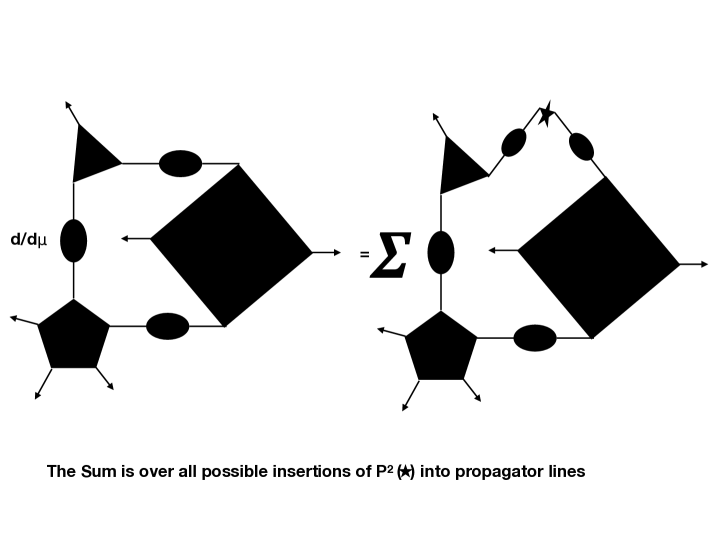
Figure 1: Graphical derivation of the scaling relation.

Differentiating a propagator gives

$$\mu\partial_{\mu}D(q)=-\frac{\mu^{1/2}}{8}{\bf q}^{2}D^{2}(q).$$ (9)

This differentiated propagator is integrated against a k + 2 point function, with momenta $q,-q,q_{1}\ldots q_{k}.$ This function is connected, but not necessarily 1PLI, because the derivative has broken open one internal propagator. In fact, every diagram for the connected k + 2 point function contributes to the scaling derivative of the 1P LI two point function. However, one must be careful about the propagators on the external legs of the k + 2 point function. On the k legs of the original 1PLI vertex, there are no propagators, so, in the popular jargon, these legs are truncated. On the integrated legs, with momentum $q$ and $-q$, we resum the Dyson series and get $W_{2}(q)$, the inverse $\mu^{1/2}{\bf q}^{2}/4+\Pi({\bf q},\omega)$ where $\Pi$ is the full polarization function, summed to all orders in the $1/N$ expansion. The easiest way to see that the combinatorics works out is to go through the functional derivation in the appendix. Defining $z=-{\rm ln}\mu$ we get an exact equation

$$\partial_{z}\Gamma_{k}(q_{1}\ldots q_{k})=-\frac{\mu^{1/2}}{8}\int\frac{d^{4}q}{(2\pi)^{4}}{\bf q}^{2}W_{2}(q)W_{2}(-q)W_{k+2}^{T}(q_{1}\ldots q_{k},q,-q)+\delta_{k2}\frac{\mu^{1/2}}{8}{\bf p_{1}}^{2}\delta^{4}(p_{1}+p_{2}).$$ (10)

In this equation, the connected correlator $W_{k+2}$ has all of its legs truncated because we have exhibited explicitly the external propagators on the integrated legs. Like the Schwinger-Dyson equations in models with cubic and quartic interactions, this equation relates 1PLI correlators with k points to those with a larger number of points. Since the action for the plasmon field contains vertices of all orders in $\chi$, the SD equations following from the effective action are much more complicated. In principle the scaling equation involves $\Gamma_{k+1}$ and $\Gamma_{k+2}$ , and so does not truncate. Recall however, that $\Gamma_{k}\sim N^{1-k/2}$ , plus higher orders in $1/N$ . This suggests an approximation scheme in which we replace $\Gamma_{k+1}$ and $\Gamma_{k+2}$ by their leading large $N$ approximation and get a closed system of scaling equations involving only $\Gamma_{m}$ with $m\leq k$. The simplest such approximation is a closed equation for $\Gamma_{2}$ :

$$\partial_{z}\Gamma_{2}(p)=\frac{e^{-z/2}}{4N}\int\frac{d^{4}q}{(2\pi)^{4}}{\bf q}^{2}\Gamma_{2}(q)^{-1}\Gamma_{2}(-q)^{-1}[S_{4}(q,-q,p,-p)+$$ (11)

$$S_{3}(q,-q,0)S_{3}(p,-p,0)\Gamma_{2}(0)^{-1}+S_{3}(q,p,-q-p)S_{3}(-q,-p,p+q))\Gamma_{2}(p+q)^{-1}$$ (12)

$$+S_{3}(q,-p,p-q)S_{3}(-q,p,q-p)\Gamma_{2}(p-q)^{-1}.$$ (13)

In this equation $S_{3,4}$ are the one fermion loop vertices of $S_{eff}$ stripped of their powers of $N$. The action for the Plasmon field is non-polynomial so its S-D equations are extremely complicated. The scaling equation is more analogous to the coupled boson-fermion S-D equations, but purely in terms of bosonic correlators. This equation is supplemented by the large boundary condition that $\Gamma_{2}\rightarrow\frac{{\mu}^{1/2}}{4}{\bf p}^{2}+S(q)$. The solution of the scaling equation with these boundary conditions is a complicated function of $N$ and $z$ and might capture some of the phase structure of the model at finite N . It would be particularly interesting to explore the question of whether the solution can have zero frequency singularities as the spatial momentum vanishes, since these would indicate the existence of a gapless plasmon excitation, and would be a likely sign of a quantum critical point.

The equations for $\Gamma_{3,4}$ involve $\Gamma_{5,6}$ and one can obtain a more refined approximation by making the substitution $\Gamma_{5,6}\rightarrow S_{5,6}$ . This gives a highly non-linear set of coupled equations for $\Gamma_{2,3,4}$. One would imagine that this second set of equations captures much of the low energy dynamics of the HEG. High point correlation functions contain only rather complicated multi- plasmon interactions, and probably do not contribute much to the coarse grained properties studied in experiment. Approximating them by their leading order large N , behavior which is also dominant in the high density limit, seems quite innocuous. Once one has chosen one of these approximation schemes, one computes the plasmon effective action by using the solutions to compute the first few terms in the $\phi$ expansion and approximating the rest by their leading large $N$ behavior. One then has a classical variational problem to solve in order to find the Born-Oppenheimer potential. It seems clear that any serious attack on these equations will have to be numerical, but perhaps analytical insight can be gained by looking for solutions with some kind of scaling behavior.

4 Conclusions

We have proposed a sequence of approximation schemes, each a refinement of the $1/N$ expansion for the HEG. The simplest of these, which is a closed equation for the two point function of the plasmon field, simply related to the density density correlation function, deserves the most attention. One should try to analyze the possibility of a gapless plasmon and or scale invariant behavior. More straightforwardly, one can try to solve the equation numerically. The unknown function depends on three variables, and is a simple evolution equation in one of them. It remains to be seen how difficult a numerical challenge this will be. It s also important to find the corresponding set of equations in the Wigner crystal phase of the model. The background classical solution provides an additional breaking of the scale symmetry we ve used, and various contributions to the scaling equations that vanished because of exact moment conservation will now have umklapp contributions. The equations will be much more complex, but might be revealing. We could also try to generalize our analysis to phases of the system with $SU(N)$ breaking, since quantum Monte Carlo Methods seem to indicate that such phases occur for $N=2$. There s a very general argument that breaking to $SU(M)\times SU(N-M)$ is only possible at large $N$ when $M$ is of order $1$. The free energy of the model scales like $N$ at large $N$ , so the system cannot have more than $o(N)$ Goldstone bosons. Large N semi-classical analysis does not show any instability in these Goldstone directions. If the approximate scaling identities do detect the broken symmetry phase, that would be strong evidence for their utility.

5 Appendix: Functional Derivation of the Scaling Equations

The action for the large N fluctuation field $\chi$ is

$$S_{eff}=\frac{\mu^{1/2}}{4}\int d^{3}y\ ds[\chi\nabla_{y}^{2}\chi]+N{\rm ln\ det}\ (\partial_{s}-\nabla_{y}^{2}/2+1+i\frac{\chi}{\sqrt{N}})+\int d^{3}y\ dsJ\chi.$$ (14)

The derivation of the scaling equations is now straightforward. The generating functional $Z[J]$ is the ratio of the functional integral with this action, and that with $J=0$. Thus ($\mu=e^{-z}$)

$$Z^{-1}\partial_{z}Z=\frac{\mu^{1/2}}{8}\int d^{3}y\ ds\nabla_{y}^{2}[Z^{-1}\frac{\delta^{2}Z}{\delta J(y)\delta J(y)}-\frac{\delta^{2}Z}{\delta J(y)\delta J(y)}_{J=0}].$$ (15)

In this equation $y$ is the four vector $(s,{\bf y})$ and the action of $\nabla_{y}^{2}$ on the coincident point two point function is defined by taking a limit of its action for non-coincident points. These terms are not integrals of total derivatives, and are better understood in momentum space. The second term in square brackets is independent of $J$, and will disappear when we look at equations for connected correlation functions.

We do this by writing $Z=e^{W}$ and differentiating with respect to $J$.

$$\partial_{z}W=\frac{\mu^{1/2}}{8}\int d^{3}y\ ds\nabla_{y}^{2}[\frac{\delta^{2}W}{\delta J(y)\delta J(y)}+\frac{\delta W}{\delta J(y)}\frac{\delta W}{\delta J(y)}].$$ (16)

Knowledgeable readers will notice the structural relation between these equations and the Wegner-Wilson-Polchinski exact renormalization group equations. If we rewrite the equations for the generating functional of 1PLI correlators, the second term in brackets only contributes to the equation for the two point function. In terms of the 1PLI generating functional our equation reads

$$\partial_{z}[\Gamma[\chi_{c}]-\int d^{4}q\ \chi_{c}(q)\frac{\delta\Gamma}{\delta\chi_{c}(q)}]=\int\frac{d^{4}q}{(2\pi)^{4}}{\bf q}^{2}[\frac{\delta^{2}W}{\delta\chi_{c}(q)\delta\chi_{c}(-q)}+\chi_{c}(q)\chi_{c}(-q)].$$ (17)

we havewritten this in momentum space because it clarifies the action of $\nabla^{2}$ on the right hand side and because it simplifies our integral equations. If we take $k$ derivatives with respect to $\chi_{c}$ on the left hand side, we get $(1-k)$ times the k-point 1PLI vertex. Recalling that $\frac{\delta J(p)}{\delta\chi_{c}(q)}=W_{2}^{-1}(p,q)$ (where the inverse is meant in the sense of integral operators) we see that we can write the equations as

$$(1-k)\partial_{z}\Gamma_{k}(p_{1},\ldots p_{k})=\int\frac{d^{4}q}{(2\pi)^{4}}{\bf q}^{2}[W_{2}(q)W_{2}(-q)W_{k}^{T}(q,-q,p_{1},\ldots p_{k})]+\delta_{k2}\frac{e^{-z/2}}{8}{\bf p_{1}}^{2}\delta^{4}(p_{1}+p_{2}).$$ (18)

$W_{k}^{T}$ is the connected $k-$ point function with all of its legs truncated. It has a tree diagram expansion involving all of the $\Gamma_{l}$ with $l\leq k$.

Like Schwinger-Dyson equations in theories with cubic and quartic interactions, this hierarchy relates the infinite set of 1PLI correlators to each other. However, we can truncate it at any $k$ by approximating $\Gamma_{k+1}$ and $\Gamma_{k+2}$ by $N^{1-k/2}S_{k+1}$ and $N^{1/2-k/2}S_{k+2}$, and obtain a closed set of equations. The equation in the text is what we obtain for the $k=2$ truncation.

Acknowledgments
The work of T.Banks is NOT supported by the Department of Energy, the NSF, the Simons Foundation, the Templeton Foundation or FQXI. I’d like to thank Bingnan Zhang for proofreading the manuscript and correcting a number of errors.

References

- [1] Yi-Kuo Yu, “Derivation of the Density Functional via Effective Action” arXiv:09100670v3[cond-matt.other] .
- [2] Hohenberg, P.; Kohn, W. (1964). ”Inhomogeneous Electron Gas”. Physical Review. 136 (3B): B864. Bibcode:1964PhRv..136..864H. doi:10.1103/PhysRev.136.B864.
- [3] T. Banks, “Density Functional Theory for Field Theorists I,” arXiv:1503.02925 [cond-mat.mtrl-sci].