Sparse Blind Deconvolution for Distributed Radar Autofocus Imaging

Abstract

A common problem that arises in radar imaging systems, especially those mounted on mobile platforms, is antenna position ambiguity. Approaches to resolve this ambiguity and correct position errors are generally known as radar autofocus. Common techniques that attempt to resolve the antenna ambiguity generally assume an unknown gain and phase error afflicting the radar measurements. However, ensuring identifiability and tractability of the unknown error imposes strict restrictions on the allowable antenna perturbations. Furthermore, these techniques are often not applicable in near-field imaging, where mapping the position ambiguity to phase errors breaks down.

In this paper, we propose an alternate formulation where the position error of each antenna is mapped to a spatial shift operator in the image-domain. Thus, the radar autofocus problem becomes a multichannel blind deconvolution problem, in which the radar measurements correspond to observations of a static radar image that is convolved with the spatial shift kernel associated with each antenna. To solve the reformulated problem, we also develop a block coordinate descent framework that leverages the sparsity and piece-wise smoothness of the radar scene, as well as the one-sparse property of the two dimensional shift kernels. We evaluate the performance of our approach using both simulated and experimental radar measurements, and demonstrate its superior performance compared to state-of-the-art methods.

I Introduction

High resolution radar imaging has become essential in a variety of remote sensing applications. While the resolution of the imaging platform in the down-range direction is primarily a function of the frequency and bandwidth of the transmitted pulse, the resolution along the cross-range (azimuth) direction depends on the aperture, i.e., the size of the radar array. In order to achieve the large aperture required in modern applications, practical systems deploy and distribute over a large area one or more, often mobile, antennas or antenna arrays, each having a relatively small aperture. The larger aperture is achieved by the virtual array formed over the large area of deployment and motion of the antennas.

A multi-antenna distributed setup further reduces the operational and maintenance costs, allows for flexibility of platform placement, and provides robustness to sensor failures. Leveraging prior knowledge of the scene, such as sparsity, the precise knowledge of the antenna positions along with a full synchronization of received signals has been shown to significantly improve the radar imaging resolution [2, 3, 4, 5].

A fundamental challenge that arises in distributed array imaging is the uncertainty in the exact positions of the transmitting and receiving antennas. Advanced positioning and navigation systems, such as the global navigation satellite system (GPS/GNSS) and the inertial navigation system (INS), generally provide reasonably accurate but not exact location information. The remaining uncertainty in the true antenna positions can still span multiple wavelengths. As a result, if the inexact antenna positions are used as-is in the imaging process, the received signal is distorted, effectively contaminated with a gain and phase ambiguity. Consequently, if the position perturbation is not compensated for, conventional reconstruction techniques produce out-of-focus radar images. A detailed analysis of antenna position errors in bistatic synthetic arrays can be found in [6].

There is extensive literature addressing the radar autofocus problem by developing tools that compensate for antenna position errors [7, 8, 9, 10, 11, 12]. In some cases, the underlying structure of the radar image, such as its sparsity, is exploited to limit the solution space and produce higher quality reconstructions [13, 14, 15, 16, 17, 18, 19]. Instead of estimating the position error, most techniques estimate an equivalent set of frequency-domain gain and phase errors in the measured signal, i.e., model the effect of the position error as a linear time-invariant filter. One advantage of these techniques is that they can often be directly combined with conventional imaging methods in the processing pipeline. However, converting the problem to a phase recovery one often poses severe restrictions on the applicability of solutions in practical applications.

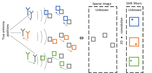
Figure 1: Position ambiguity of the radar antennas induces an image-domain convolution model.

I-A Main contributions

In contrast to earlier approaches, our work fundamentally re-examines the acquisition model. Specifically, we study the general high resolution radar imaging problem of recovering a sparse stationary image of a scene under position ambiguity of the antennas. We demonstrate in Section II that determining the antenna position ambiguity is equivalent to a blind deconvolution problem in the image domain. In particular, we assert that measurements acquired using an antenna in an assumed position, but with unknown position error, are equal to measurements of the scene convolved with a two-dimensional unknown shift kernel, using an antenna without position error. Figure 1 illustrates the key intuition of our formulation. The unknown kernel shifting the scene mirrors the unknown shift error of the antenna, relative to its assumed position. In addition, we prove that the image-domain convolution model is exact if the transmitting and receiving antennas are affected by the same position error, a common occurrence in practice, for example if transmission and reception uses the same antenna or if both antennas are mounted on the same platform.

In addition to our novel formulation, we also propose in Section III a block-coordinate descent algorithm to efficiently solve the sparse blind deconvolution problem in the image domain. We validate our approach using numerical simulations and experimental results that demonstrate their effectiveness. Figure 2 provides an example of the improvements due to our approach. In this example, the scene in Figure 2(a), including three reflective objects, is imaged using a distributed array with 4 mobile antennas and position perturbations. Ignoring position errors produces significant artifacts, as shown in Figure 2(b). While conventional methods improve imaging performance, as shown in Figure 2(c), there are still missing targets and artifacts. Our approach is able to recover the scene, as demonstrated in Figure 2(d). The performance improvement is consistent in a variety of sensing conditions and very large position errors. More details on this and other experiments are provided in Section IV.

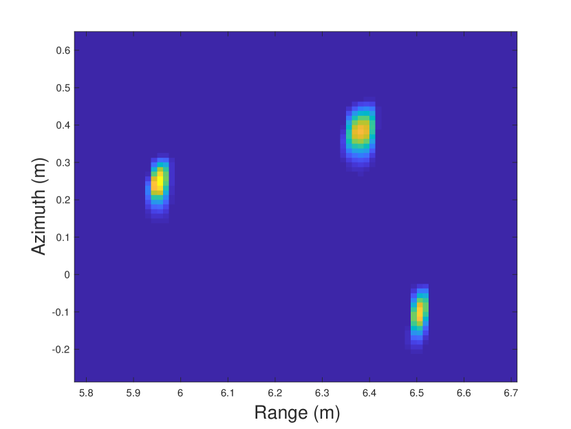
(a)

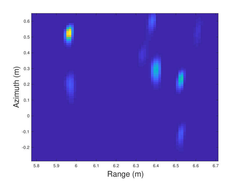
(b)

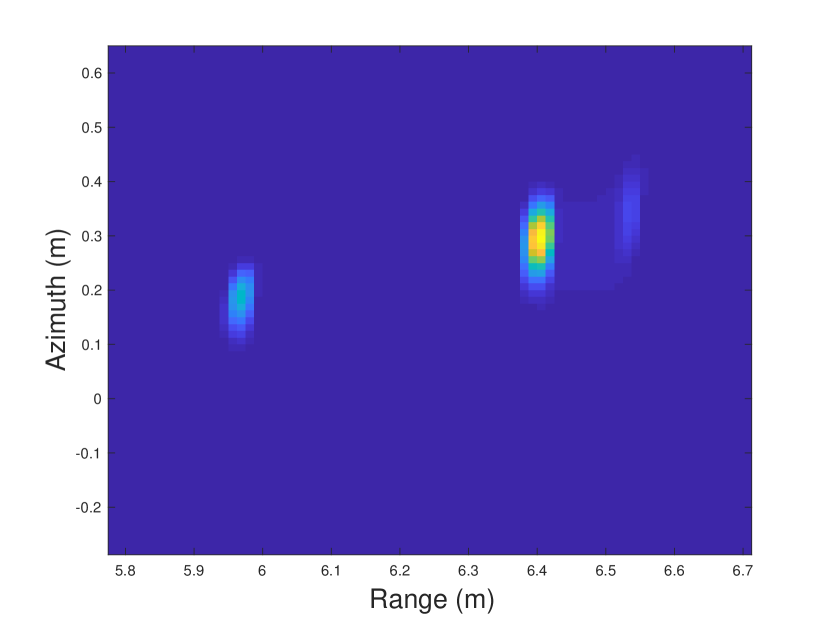
(c)

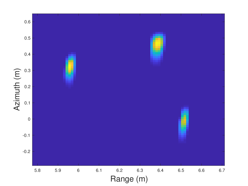
(d)

Figure 2: (a)–(b) Sparse recovery of radar images without autofocusing obtained using (a) the correct antenna positions, and (b) the incorrect antenna positions. (c)–(d) Autofocus results using blind deconvolution according to (c) the time-domain convolution model; and (d) using the proposed sparse blind deconvolution and the image-domain convolution model.

I-B Background and Related Work

In its most general formulation, using an arbitrary gain and phase error to model the data error in the frequency domain, the radar autofocus problem is ill-posed. The overwhelming majority of the literature addresses this ill-posedness by imposing constraints on the dimensionality of the error. These constraints include constant phase error assumptions or restricted subspace assumptions [9, 20, 21, 22, 23], and sparsity assumptions [13, 15, 18, 17, 19]. While some of these assumptions may be valid under specific conditions of the measurement process, they do not necessarily apply to the general radar imaging problem.

In the context of autofocus using synthetic arrays, well established approaches include phase gradient autofocus (PGA) [7] and sharpness optimization autofocus techniques [8, 24, 25, 26]. The PGA approach estimates the derivative of the phase error using a minimum variance estimator. The underlying assumption is that individual targets in the scene exhibit the same phase error. Alternatively, contrast optimization techniques, optimize a sharpness function of the reconstructed image. The radar imaging operators of each measurement are assumed to be invertible and the phase errors are assumed to impact individual columns in the radar image.

Another approach championed in [11, 20, 27] is the multichannel autofocus (MCA) and Fourier domain multichannel autofocus (FMCA). Both techniques develop solutions that map the autofocus problem into a constant modulus quadratic program (CMQP) that is solved using subspace identification methods or semidefinite relaxation. In these approaches, it is assumed that the measurements are acquired at specific look angles. For each look angle, the measurements are impacted by an unknown delay, resulting in a constant unknown phase shift under a narrow band assumption. The delays, and their associated phases, change between different look angles. Such a model has two limitations for high resolution radar imaging. The first limitation is the assumption that a radar measurement from one antenna position receives reflections from a single ray along a single scan angle. In the general radar imaging setting, a single radar measurement can receive reflections from a large spatial area in the scene. The second limitation is related to the first and materializes in the form of restricting the phase ambiguity to a spatial shift along the radial line. In fact, we prove in this paper that, in the general radar setting, the phase ambiguity is realized instead as a two-dimensional spatial shift of the radar image.

More generally, the radar autofocus problem can be viewed as a multichannel blind deconvolution problem, where the distortions due to position errors can be considered as unknown channels acting on the signals that are received in each antenna. Blind deconvolution attempts to separate a signal and a channel from their convolved mixture, i.e., their product in the frequency domain, using assumptions on each of the two. The multi-channel version considers multiple channels affecting the same signal. Solutions to the general multichannel blind deconvolution problem have existed in the literature since the 1990s [28, 29, 30, 31, 32].

More recent research has focused on convex formulations and recovery guarantees. The seminal work of Ahmed, Recht, and Romberg [33] proposed a convex formulation of the single-channel problem, recovering the two signals by lifting the problem to a frequency-domain outer-product space. Under this formulation, the acquired data are linear measurements of an unknown rank-one matrix to be recovered. The unknown channel and signal vectors are obtained by factoring this rank-one matrix to its components. The authors presented a theoretical analysis of the recovery guarantees of the lifted problem when both unknowns exist in low dimensional subspaces, and for a generic linear acquisition system. The analysis was later generalized by Li and Strohmer [34] using the SparseLift technique to the case where the signal is sparse and exists on a union of subspaces spanned by an unknown subset of the columns of a dictionary that has measurement concentration properties. Along a similar track, Li, Lee, and Bresler [35, 36] analyzed the identifiability properties of these bilinear inverse problems. The problem of recovering a sparse signal from diverse convolutive measurements was also studied by Ahmed and Demanet [37] under the assumption that the convolution filters are members of known low-dimensional random subspaces.

Another convex approach that has been studied in [38, 39, 40, 41, 42, 43] recasts blind deconvolution as a linear least squares problem, thus enjoying lower computational complexity compared to the lifting approach when certain conditions are satisfied. Finally, we point out that other nonconvex formulations with recovery guarantees have been studied in [44, 45, 46, 47]. A key difference in this prior work and our model is that, in the terminology of blind deconvolution, both our signals and our channels are sparse in the same domain, thus violating most common assumptions necessary for recovery guarantees. On the other hand, our algorithm is able to exploit some additional diversity due to the multi-channel nature of our formulation.

I-C Notation

Throughout the text, lower case bold face letters ${\mathbf{x}}$ denote vectors and upper case bold face letters ${\mathbf{X}}$ denote matrices. Sets are denoted by calligraphic upper case letters $\mathcal{B}$ or upper case Greek letters $\Omega$. Italicized bold upper case letters ${\bm{R}}(\cdot)$ refer to functions that act on vector spaces. We use ${\mathbf{F}}_{1}$ and ${\mathbf{F}}_{2}$ to refer to the one-dimensional and two-dimensional Fourier transform matrices, respectively. The matrix ${\mathbf{D}}_{{\mathbf{x}}}$ is used to indicate a diagonal matrix with the vector ${\mathbf{x}}$ on its main diagonal. Superscripts ^T and ^H refer to the transpose and the Hermitian transpose of matrices, respectively. The function $\delta({\bm{l}}+{\bm{e}})$ refers to the Dirac delta function of the variable ${\bm{l}}$ delayed by the quantity ${\bm{e}}$. The $\ell_{1}$ norm of a vector ${\mathbf{x}}$ is defined as the sum of its absolute values, i.e., $\|{\mathbf{x}}\|_{1}=\sum\limits_{j}|{\mathbf{x}}(j)|$. The $\ell_{2}$ norm of a vector is equal to the square root of the sum of squares of the vector, i.e., $\|{\mathbf{x}}\|_{2}=\sqrt{\sum\limits_{j}|{\mathbf{x}}(j)|^{2}}$.

II Problem Formulation

II-A Signal model

We consider a two-dimensional radar imaging scenario in which $M$ distributed antennas are used to detect $K$ targets. A three-dimensional generalization is straightforward, but we avoid it here for simplicity of exposition. The targets are located within a spatial region of interest that is discretized on a grid $\Omega\subset\mathbb{R}^{2},|\Omega|=N,$ and $N=N_{x}\times N_{y}$ with $N_{x}$ and $N_{y}$ specifying the number of grid points in the horizontal and vertical directions. We use ${\bm{l}}\in\Omega$ to denote the index of spatial positions, i.e., of grid-points in $\Omega$. We assume that the grid is sufficiently fine, that off-grid errors are negligible, and that there exists a single reflector in each grid point.

Let $\Gamma\subset\mathbb{R}^{2},|\Gamma|=M$ be the set of all the spatial locations of the $M$ antennas. Note that the antennas may be located anywhere, inside or outside of the grid, and not necessarily on a grid point. Without loss of generality, we shall assume that a subset of the antennas act as transmitter/receivers while the remaining antennas are only receivers. A transmitting antenna at position ${\bm{r}}\in\Gamma$ emits a time-domain pulse $p(t)$ with frequency spectrum $P(\omega)$, where $\omega=2\pi f$ is the angular frequency and $f\in\mathcal{B}$ is the ordinary frequency in the signal bandwidth $\mathcal{B},|\mathcal{B}|=F$. The received signal at antenna position ${\bm{r}}^{\prime}\in\Gamma$ due to the scattering of the transmitted pulse by a target located at position ${\bm{l}}\in\Omega$ is given by [48]

$$Y(\omega,{\bm{l}},{\bm{r}},{\bm{r}}^{\prime})=P(\omega)G(\omega,{\bm{r}},{\bm{r}}^{\prime},{\bm{l}})X({\bm{l}})+N(\omega),$$ (1)

where $X({\bm{l}})\in\mathbb{C}$ is the scene reflectivity at location ${\bm{l}}$, $N(\omega)$ is a noise component, and $G(\omega,{\bm{r}},{\bm{r}}^{\prime},{\bm{l}})$ is the propagation gain characterized by

$$G(\omega,{\bm{r}},{\bm{r}}^{\prime},{\bm{l}})=a({\bm{r}},{\bm{r}}^{\prime},{\bm{l}}){\mathrm{e}}^{-i\omega\frac{\|{\bm{r}}-{\bm{l}}\|_{2}+\|{\bm{r}}^{\prime}-{\bm{l}}\|_{2}}{c}},$$ (2)

where $a({\bm{r}},{\bm{r}}^{\prime},{\bm{l}})$ is the magnitude attenuation, ${\mathrm{e}}^{-i\omega\frac{\|{\bm{r}}-{\bm{l}}\|_{2}+\|{\bm{r}}^{\prime}-{\bm{l}}\|_{2}}{c}}$ is the phase change due to the transmission delay, and $c$ denotes the speed of light.

A typical scene comprises of multiple reflectors, at different locations ${\bm{l}}\in\Omega$. If we assume no shadowing and no multiple reflections, the received data for receiver-transmitter pair is the sum of (1) over all ${\bm{l}}$ in which reflectors are present. To compact notation, we use ${\mathbf{x}}\in\mathbb{C}^{N}$ to denote the vectorized reflectivity of the scene at all grid points in $\Omega$, with empty grid points having zero reflectivity. Thus, the received signal in (1) at all frequencies $\omega$ can then be written in vector form ${\mathbf{y}}({\bm{r}},{\bm{r}}^{\prime})\in\mathbb{C}^{F}$ as follows

$${\mathbf{y}}({\bm{r}},{\bm{r}}^{\prime})={\mathbf{A}}({\bm{r}},{\bm{r}}^{\prime}){\mathbf{x}}+{\mathbf{n}}({\bm{r}},{\bm{r}}^{\prime}),$$ (3)

where ${\mathbf{A}}({\bm{r}},{\bm{r}}^{\prime})\in\mathbb{C}^{F\times N}$ includes $P(\omega)$ and $G(\omega,{\bm{r}},{\bm{r}}^{\prime},{\bm{l}})$ and denotes the radar imaging operator corresponding to the transmitter and receiver pair at positions ${\bm{r}}$ and ${\bm{r}}^{\prime}$, respectively, and ${\mathbf{n}}({\bm{r}},{\bm{r}}^{\prime})$ is the noise component.

II-B Imaging under position uncertainty

Using (3) to estimate the scene reflectivity ${\mathbf{x}}$ from measurements ${\mathbf{y}}({\bm{r}},{\bm{r}}^{\prime})$ requires exact knowledge of the imaging operator ${\mathbf{A}}({\bm{r}},{\bm{r}}^{\prime})$, and consequently, the antenna positions ${\bm{r}}$ and ${\bm{r}}^{\prime}$. However, positioning errors commonly occur in practice, especially in distributed radar settings which rely on inaccurate global positioning systems or inertial navigation systems.

To model the effect of position errors, we consider transmitter-receiver pairs indexed by $m$, positioned at $({\bm{r}}_{m},{\bm{r}}^{\prime}_{m})$. We denote the measurement vector at the assumed position of the pair and the corresponding imaging operator using ${\mathbf{y}}_{m}:={\mathbf{y}}({\bm{r}}_{m},{\bm{r}}^{\prime}_{m})$ and ${\mathbf{A}}_{m}:={\mathbf{A}}({\bm{r}}_{m},{\bm{r}}^{\prime}_{m})$, respectively. We use $\widetilde{{\bm{r}}}_{m}={\bm{r}}_{m}+{\bm{e}}_{m}$ and $\widetilde{{\bm{r}}}^{\prime}_{m}={\bm{r}}^{\prime}_{m}+{\bm{e}}^{\prime}_{m}$ to denote the actual positions of the transmitter and receiver, respectively, where ${\bm{e}}_{m}$ and ${\bm{e}}^{\prime}_{m}$ denote the corresponding positioning errors.

The actual received antenna measurement $\widetilde{{\mathbf{y}}}_{m}:={\mathbf{y}}(\widetilde{{\bm{r}}}_{m},\widetilde{{\bm{r}}}^{\prime}_{m})$ observes the scene reflectivity ${\mathbf{x}}$ through the perturbed imaging operator $\widetilde{{\mathbf{A}}}_{m}:={\mathbf{A}}(\widetilde{{\bm{r}}}_{m},\widetilde{{\bm{r}}}^{\prime}_{m})$, i.e.,

$$\widetilde{{\mathbf{y}}}_{m}=\widetilde{{\mathbf{A}}}_{m}{\mathbf{x}}+{\mathbf{n}}_{m}.$$ (4)

Since the operator $\widetilde{{\mathbf{A}}}_{m}$ is unknown, we need to model the received measurements $\widetilde{{\mathbf{y}}}_{m}$ as a function of ${\mathbf{A}}_{m}$ and ${\mathbf{x}}$.

II-B1 Convolution in the measurement-domain

Standard approaches for radar autofocus use a gain and phase correction in the measurements’ frequency domain to describe $\widetilde{{\mathbf{y}}}_{m}$ in terms of ${\mathbf{A}}_{m}$ and ${\mathbf{x}}$. More precisely, let $\widehat{{\mathbf{g}}}_{m}\in\mathbb{C}^{F}$ be a complex valued vector corresponding to the Fourier transform of a time-domain kernel ${\mathbf{g}}_{m}\in\mathbb{R}^{M}$, i.e, ${\mathbf{g}}_{m}={\mathbf{F}}_{1}^{\mathsf{H}}\widehat{{\mathbf{g}}}_{m}$. The received frequency-domain measurements are expressed as

$$\widetilde{{\mathbf{y}}}_{m}={\mathbf{D}}_{\widehat{{\mathbf{g}}}_{m}}{\mathbf{A}}_{m}{\mathbf{x}}+{\mathbf{n}}_{m},$$ (5)

where ${\mathbf{D}}_{\widehat{{\mathbf{g}}}_{m}}$ is a diagonal matrix with $\widehat{{\mathbf{g}}}_{m}$ on its diagonal entries, i.e., modulates the acquired frequency-domain data. In other words, the position error is assumed to affect the received signal through a time-domain convolution with ${\mathbf{g}}_{m}$. Given $M$ measurements $\widetilde{{\mathbf{y}}}_{m},m\in\{1\dots M\}$, the radar autofocus problem is regarded as a bilinear inverse problem in both the reflectivity image ${\mathbf{x}}$ and the frequency-domain phase correction vectors $\widehat{{\mathbf{g}}}_{m}$ for all $m$.

Notice that the system in (5) has $F$ equations with $F+N$ unknowns, which makes it severely ill-posed. Even in the case where ${\mathbf{x}}$ is sparse, the problem remains ill-posed since a general phase correction vector $\widehat{{\mathbf{g}}}_{m}$ continues to have $F$ degrees of freedom. In order to make the problem tractable, the kernels ${\mathbf{g}}_{m}={\mathbf{F}}_{1}^{\mathsf{H}}\widehat{{\mathbf{g}}}_{m}$ are often assumed to be shift kernels, which reduces the degrees of freedom to a singe phase angle per transmitter-receiver pair. However, the approximation that ${\mathbf{g}}_{m}$ is a shift operator is only valid in the far field regime, where the position error can be approximated by a one dimensional shift in the down-range direction of the virtual antenna array, or if the scene only contains a single reflector.

Most work in the self-calibration and radar autofocus literature considers the measurement-domain convolution model in (5) with some important simplifications. For instance, the convolution kernels ${\mathbf{g}}_{m}$ are assumed to be approximate shift kernels and therefore sparse in the time-domain. Specifically, the simplification allows the kernels ${\mathbf{g}}_{m}$ to be restricted to a lower $d$-dimensional subspace spanned by the columns of a basis matrix ${\mathbf{B}}\in\mathbb{C}^{F\times d},d<F$. Combining all measurements $M$ into a single system of equations, we obtain the following bilinear inverse problem

$$\overline{{\mathbf{y}}}={\mathbf{D}}_{\widehat{\overline{{\mathbf{g}}}}}\overline{{\mathbf{A}}}{\mathbf{x}}+\overline{{\mathbf{n}}},$$ (6)

where the over-line notation indicates stacking the $M$ vectors (or matrices) vertically into a single vector (or matrix), for example $\overline{{\mathbf{y}}}=\left[\begin{array}[]{c}{\mathbf{y}}_{1}\\ \vdots\\ {\mathbf{y}}_{M}\end{array}\right]$ and $\overline{{\mathbf{A}}}=\left[\begin{array}[]{c}{\mathbf{A}}_{1}\\ \vdots\\ {\mathbf{A}}_{M}\end{array}\right]$. Note that with this formulation, the vector $\overline{{\mathbf{g}}}$ belongs to the $Md$-dimensional subspace in $\mathbb{C}^{MF}$ spanned by the basis matrix

$$\overline{{\mathbf{B}}}=\left[\begin{array}[]{cccc}{\mathbf{B}}&\mathbf{0}&\ldots&\mathbf{0}\\ \mathbf{0}&{\mathbf{B}}&&\mathbf{0}\\ \vdots&&\ddots&\\ \mathbf{0}&\mathbf{0}&\ldots&{\mathbf{B}}\end{array}\right]\in\mathbb{C}^{MF\times Md},$$

where $\mathbf{0}$ is the $F\times d$ all zero matrix. Under this scenario, Ling and Strohmer [34] proposed the SparseLift problem which casts the blind deconvolution problem as a convex sparse recovery program that estimates the sparse matrix ${\mathbf{X}}=\overline{{\mathbf{g}}}{\mathbf{x}}^{\mathsf{H}}$ in the lifted space of the outer products of $\overline{{\mathbf{g}}}$ and ${\mathbf{x}}$. However, as the number of measurements and the dimensions of the parameters increase, the SparseLift formulation can quickly become intractable to solve. Alternatively, Mansour et al. [49] proposed a stochastic gradient descent approach for solving the nonconvex variation of (6) in the context of through-the-wall-radar-imaging.

Other simplifications in the literature assume the operators ${\mathbf{A}}_{m}={\mathbf{A}}$ to be fixed for all $m$. In this case, the measurements $\widetilde{{\mathbf{y}}}_{m}$ represent multiple measurements of a single vector ${\mathbf{z}}:={\mathbf{A}}{\mathbf{x}}$ observed through diverse channels $\widehat{{\mathbf{g}}}_{m}$, i.e.,

$$\widetilde{{\mathbf{y}}}_{m}={\mathbf{D}}_{{\mathbf{z}}}\widehat{{\mathbf{g}}}_{m}.$$ (7)

Existing solutions to (7) range from solving for a low rank matrix in the lifted space of the variables ${\mathbf{z}}$ and $\widehat{{\mathbf{g}}}_{m}$ [33, 34, 35, 37]; reformulating the problem as a linear least squares problem [38, 39, 40, 41, 42, 43]; or utilizing subspace identification techniques [11, 20, 27].

While the simplifications described above can apply to special cases of autofocusing and self-calibration problems, they are not necessarily satisfied in general radar autofocus problems as we demonstrated in the previous section. We discuss next the image-domain blind deconvolution model and propose a reconstruction algorithm to solve the problem.

II-B2 Convolution in the image-domain

A key contribution of our work is moving the convolution with the shift kernel from the measurement domain to the image domain. More precisely, let ${\mathbf{h}}_{m}\in\mathbb{R}^{N_{h}^{2}},N_{h}\leq\min\{N_{x},N_{y}\}$ be a vectorized two-dimensional shift kernel of size $N_{h}\times N_{h}$. Under the new model, the received signal of the antenna pair indexed by $m$ is written as

$$\widetilde{{\mathbf{y}}}_{m}={\mathbf{A}}_{m}\left({\mathbf{x}}*{\mathbf{h}}_{m}\right)+{\mathbf{n}}_{m},$$ (8)

where $*$ here denotes the two-dimensional convolution of the image with the kernel.

We prove in Proposition 1 that when the transmitting and receiving antennas are affected by the same position ambiguity, the convolution kernel ${\mathbf{h}}_{m}$ is strictly a spatial shift kernel with a single nonzero entry equal to one. This situation is prevalent in systems where the transmitting and receiving antennas are collocated. The system in (8) may still be underdetermined with $F$ equations and $N_{h}^{2}+N$ unknowns. However, given enough measurements, it should be possible to recover ${\mathbf{x}}$ and all shift kernels ${\mathbf{h}}_{m}$ by utilizing an appropriate regularization for each. In the next section, we demonstrate the appropriateness of the image-domain convolution in (8) compared to the measurement-domain convolution in (5) through an illustrative example.

Proposition 1.

Let $\widetilde{{\mathbf{y}}}_{m}:=\widetilde{{\mathbf{A}}}_{m}{\mathbf{x}},$ where ${\mathbf{x}}$ is a radar image defined over a spatial domain $\Omega$. Denote by ${\bm{e}}_{m}$ and ${\bm{e}}^{\prime}_{m}$ the position ambiguities for the transmitter and receiver antenna pair indexed by $m$.

If ${\bm{e}}^{\prime}_{m}={\bm{e}}_{m}$ and ${\mathbf{x}}$ is zero valued within a boundary of width ${\bm{e}}_{m}$ inside $\Omega$, then there exists a spatially shifted image $\widetilde{{\bm{x}}}({\bm{l}})=\delta({\bm{l}}+{\bm{e}}_{m})*{\bm{x}}({\bm{l}}),\forall{\bm{l}}\in\Omega$ such that $\widetilde{{\mathbf{y}}}_{m}={\mathbf{A}}_{m}\widetilde{{\mathbf{x}}},$ where $\delta({\bm{l}}+{\bm{e}}_{m})$ is the two dimensional shift kernel.

Otherwise, if ${\bm{e}}^{\prime}_{m}={\bm{e}}_{m}+{\bm{d}}_{m}$ with $\|{\bm{d}}_{m}\|_{2}\leq\Delta$, then the approximation $\widetilde{{\mathbf{y}}}_{m}\approx{\mathbf{A}}_{m}\widetilde{{\mathbf{x}}}$ incurs a phase error bounded by ${\mathrm{e}}^{\pm i\omega\Delta/c}$ for each frequency $\omega$.

Proof.

Consider the received signal $\widetilde{{\mathbf{y}}}(\omega)$ at an arbitrary frequency $\omega$ in the bandwidth of the radar pulse. Ignoring the amplitude attenuation, the received signal at perturbed antenna positions $\widetilde{{\bm{r}}},\widetilde{{\bm{r}}}^{\prime}$ is given by

$$\widetilde{{\mathbf{y}}}(\omega)=\widetilde{{\mathbf{A}}}(\omega){\mathbf{x}}=\sum\limits_{{\bm{l}}\in\Omega}{\mathrm{e}}^{-i\omega\frac{\|\widetilde{{\bm{r}}}-{\bm{l}}\|_{2}+\|\widetilde{{\bm{r}}}^{\prime}-{\bm{l}}\|_{2}}{c}}{\mathbf{x}}({\bm{l}}),$$ (9)

where $\widetilde{{\mathbf{A}}}_{m}(\omega)$ is the row of $\widetilde{{\mathbf{A}}}$ corresponding to the frequency $\omega$. Recall that $\widetilde{{\bm{r}}}={\bm{r}}+{\bm{e}},$ $\widetilde{{\bm{r}}}^{\prime}={\bm{r}}^{\prime}+{\bm{e}}^{\prime}$. When ${\bm{e}}={\bm{e}}^{\prime}$, we have

$$\begin{array}[]{ll}\|\widetilde{{\bm{r}}}-{\bm{l}}\|_{2}+\|\widetilde{{\bm{r}}}^{\prime}-{\bm{l}}\|_{2}&=\|{\bm{r}}+{\bm{e}}-{\bm{l}}\|_{2}+\|{\bm{r}}^{\prime}+{\bm{e}}^{\prime}-{\bm{l}}\|_{2}\\ &=\|{\bm{r}}-\widetilde{{\bm{l}}}\|_{2}+\|{\bm{r}}^{\prime}-\widetilde{{\bm{l}}}\|_{2},\end{array}$$

where $\widetilde{{\bm{l}}}={\bm{l}}-{\bm{e}}$. Then the received signal $\widetilde{{\mathbf{y}}}(\omega)$ satisfies

$$\begin{array}[]{ll}\widetilde{{\mathbf{y}}}(\omega)&=\sum\limits_{{\bm{l}}\in\Omega}{\mathrm{e}}^{-i\omega\frac{\|{\bm{r}}-\widetilde{{\bm{l}}}\|_{2}+\|{\bm{r}}^{\prime}-\widetilde{{\bm{l}}}\|_{2}}{c}}{\mathbf{x}}({\bm{l}})\\ &=\sum\limits_{\widetilde{{\bm{l}}}\in\widetilde{\Omega}}{\mathrm{e}}^{-i\omega\frac{\|{\bm{r}}-\widetilde{{\bm{l}}}\|_{2}+\|{\bm{r}}^{\prime}-\widetilde{{\bm{l}}}\|_{2}}{c}}{\mathbf{x}}(\widetilde{{\bm{l}}}+{\bm{e}})\\ &=\sum\limits_{\widetilde{{\bm{l}}}\in\widetilde{\Omega}}{\mathrm{e}}^{-i\omega\frac{\|{\bm{r}}-\widetilde{{\bm{l}}}\|_{2}+\|{\bm{r}}^{\prime}-\widetilde{{\bm{l}}}\|_{2}}{c}}\left(\delta(\widetilde{{\bm{l}}}+{\bm{e}})*{\mathbf{x}}(\widetilde{{\bm{l}}})\right),\end{array}$$ (10)

where $\widetilde{\Omega}$ is a displacement of the set $\Omega$ by ${\bm{e}}$. Denote by $\widetilde{{\mathbf{x}}}(\widetilde{{\bm{l}}})=\delta(\widetilde{{\bm{l}}}+{\bm{e}})*{\mathbf{x}}(\widetilde{{\bm{l}}})$ and since the support of ${\mathbf{x}}$ is surrounded by a zero valued boundary of width ${\bm{e}}$ inside $\Omega$, we get

$$\begin{array}[]{ll}\widetilde{{\mathbf{y}}}(\omega)&=\sum\limits_{\widetilde{{\bm{l}}}\in\widetilde{\Omega}}{\mathrm{e}}^{-i\omega\frac{\|{\bm{r}}-\widetilde{{\bm{l}}}\|_{2}+\|{\bm{r}}^{\prime}-\widetilde{{\bm{l}}}\|_{2}}{c}}\widetilde{{\mathbf{x}}}(\widetilde{{\bm{l}}})\\ &=\sum\limits_{{\bm{l}}\in\Omega}{\mathrm{e}}^{-i\omega\frac{\|{\bm{r}}-{\bm{l}}\|_{2}+\|{\bm{r}}^{\prime}-{\bm{l}}\|_{2}}{c}}\widetilde{{\mathbf{x}}}({\bm{l}})\\ &={\mathbf{A}}(\omega)\widetilde{{\mathbf{x}}}({\bm{l}}).\end{array}$$ (11)

If ${\bm{e}}^{\prime}={\bm{e}}+{\bm{d}}$ for some offset ${\bm{d}},\|{\bm{d}}\|_{2}\leq\Delta$, then

$$\begin{array}[]{l}\|{\bm{r}}-\widetilde{{\bm{l}}}\|_{2}+\|{\bm{r}}^{\prime}-\widetilde{{\bm{l}}}\|_{2}-\Delta\\ \hskip 36.135pt\leq\|\widetilde{{\bm{r}}}-{\bm{l}}\|_{2}+\|\widetilde{{\bm{r}}}^{\prime}-{\bm{l}}\|_{2}\leq\\ \hskip 72.26999pt\|{\bm{r}}-\widetilde{{\bm{l}}}\|_{2}+\|{\bm{r}}^{\prime}-\widetilde{{\bm{l}}}\|_{2}+\Delta\end{array}$$

Consequently, the expression in (11) incurs a maximum phase error equal to ${\mathrm{e}}^{\pm i\omega\Delta/c}$ when ${\bm{e}}^{\prime}\neq{\bm{e}}$. ∎

II-B3 An illustrative example

We simulate a radar scene with three targets inside a region of interest $\Omega$ and generate measurements corresponding to three transmitter-receiver antennas as shown in Figure 3. The blue crosses and red circles indicate the true positions and the assumed (erroneous) positions of the antennas, respectively.

Consider first the antennas lying inside the dashed ellipse. The time-domain measurements corresponding to each of the antenna positions are shown in the top plot of Figure 4. According to the model in (5), there exists a convolutional kernel ${\mathbf{g}}$ shown in the bottom plot of Figure 4 that maps the red curve corresponding to ${\mathbf{F}}_{1}^{\mathsf{H}}{\mathbf{A}}_{m}{\mathbf{x}}$ to the blue curve corresponding to ${\mathbf{F}}_{1}^{\mathsf{H}}\widetilde{{\mathbf{A}}}_{m}{\mathbf{x}}$, where ${\mathbf{F}}_{1}$ is the one-dimensional Fourier transform. However, it is clear from the figure that ${\mathbf{g}}$ cannot be a simple shift kernel. On the other hand, consider the reflectivity images in Figure 5 (a) and (b) obtained from multiplying the received measurement $\widetilde{{\mathbf{y}}}_{m}=\widetilde{{\mathbf{A}}}_{m}{\mathbf{x}}$ by the adjoint of each of the true imaging operator $\widetilde{{\mathbf{A}}}_{m}$ and the erroneous imaging operator ${\mathbf{A}}_{m}$. Notice that there does exist a simple two-dimensional shift kernel that can be applied to the true reflectivity image ${\mathbf{x}}$ to produce the measurements $\widetilde{{\mathbf{y}}}_{m}$. To better illustrate this fact, we apply the same shift to two other antennas as shown in Figure 3 and generate the reflectivity images in Figure 5 (c) and (d) using each of the imaging operators $\widetilde{{\mathbf{A}}}_{m}$ and ${\mathbf{A}}_{m}$, respectively. The arcs visible in Figure 5 (a) and (b) become focused on the shifted target locations since the resulting virtual array has a wider aperture, which in turn reduces the null space of the resulting imaging operator.

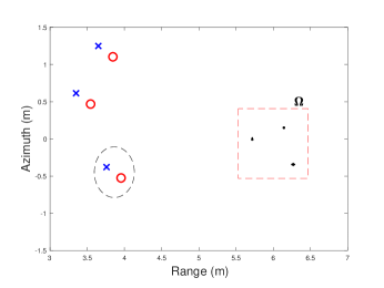
Figure 3: Illustration of an example radar scene with three antennas at the true positions marked by the blue $\times$’s and the assumed positions marked by the red circles. Three targets are observed inside the region of interest bounded by the dashed red line.

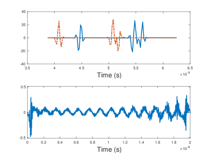
Figure 4: Top: time-domain signals observed by the third set of antennas shown in Figure 3 and highlighted by the dashed ellipse. The solid blue line corresponds to the signal observed by the location of the $\times$. The dashed red line corresponds to the signal observed by the location of the circle. Bottom: Convolution kernel that maps the red curve to the blue curve.

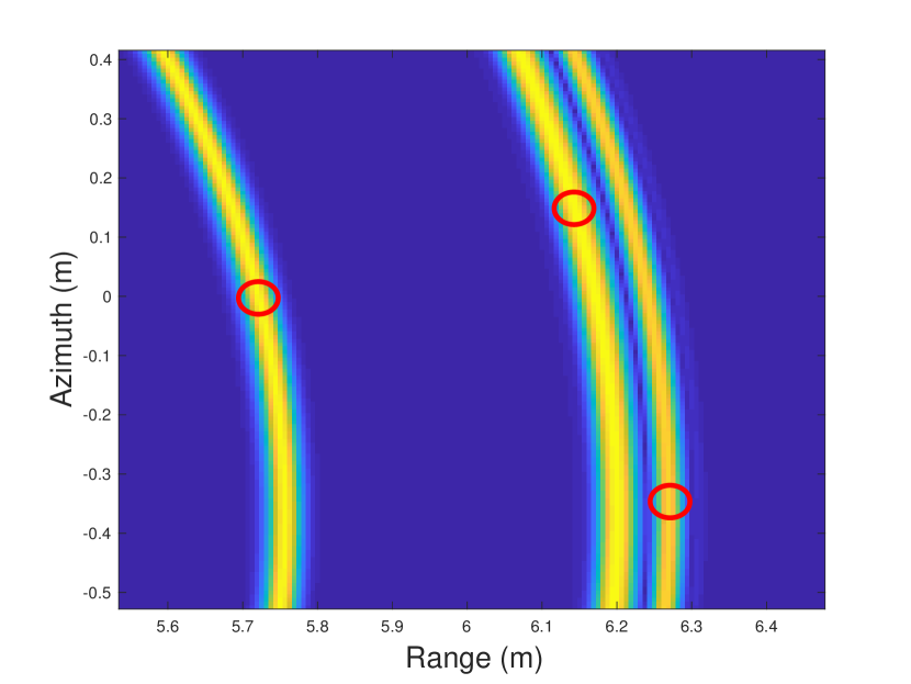
(a)

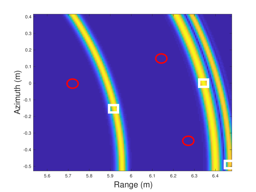
(b)

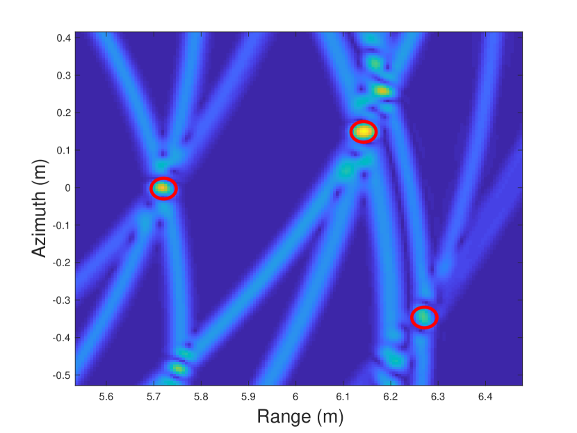
(c)

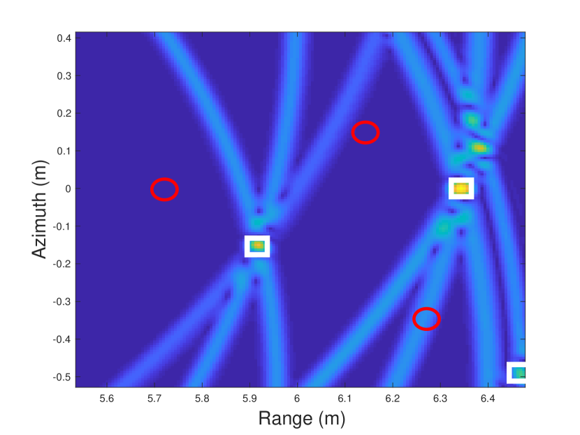
(d)

Figure 5: Imaging results obtained by applying the adjoint of the true imaging operator $\widetilde{{\mathbf{A}}}$ in (a) and (c); and the wrong imaging operator ${\mathbf{A}}$ in (b) and (d) to the received measurements. (a) and (b) show the imaging result from the single antenna measurement marked by the $\times$ in the ellipse shown in Figure 3. (c) and (d) show the imaging result from using the antenna positions marked by all three $\times$. The red circles and white squares indicate the true positions and the shifted positions of the targets, respectively.

Before ending this section, we consider again the image-domain convolution model described in (8) and expressed in the spatial Fourier domain below

$$\begin{array}[]{ll}\widetilde{{\mathbf{y}}}_{m}&={\mathbf{A}}_{m}\left({\mathbf{x}}*{\mathbf{h}}_{m}\right)+{\mathbf{n}}_{m}\\ &={\mathbf{A}}_{m}{\mathbf{F}}_{2}^{\mathsf{H}}{\mathbf{D}}_{\widehat{{\mathbf{h}}}_{m}}\widehat{{\mathbf{x}}}+{\mathbf{n}}_{m},\end{array}$$ (12)

where $\widehat{{\mathbf{h}}}_{m}={\mathbf{F}}_{2}{\mathbf{h}}_{m}$ and $\widehat{{\mathbf{x}}}={\mathbf{F}}_{2}{\mathbf{x}}$ denote the two-dimensional Fourier transforms of ${\mathbf{h}}_{m}$ and ${\mathbf{x}}$, respectively, and ${\mathbf{D}}_{\widehat{{\mathbf{h}}}_{m}}$ is the diagonal matrix with $\widehat{{\mathbf{h}}}_{m}$ on the diagonal. Notice that the convolved signal $\left({\mathbf{x}}*{\mathbf{h}}_{m}\right)$ in (12) is now observed through a linear operator ${\mathbf{A}}_{m}$ that has a large null space, making the variety of convex optimization methods in the literature developed for blind deconvolution inapplicable to this scenario. We may consider convexifying problem (12) by lifting into the variable representation ${\mathbf{X}}_{m}={\mathbf{h}}{\mathbf{x}}^{\mathsf{H}},$ such that $\widetilde{{\mathbf{y}}}_{m}={\mathbf{A}}_{m}{\mathbf{C}}\ \mathrm{vec}({\mathbf{X}}_{m}),$ where the linear operator ${\mathbf{C}}$ maps the vectorized outer-product matrix $\mathrm{vec}({\mathbf{X}}_{m})$ to the output of the convolution $\left({\mathbf{x}}*{\mathbf{h}}_{m}\right)$. However, the resulting linear operator ${\mathbf{A}}_{m}{\mathbf{C}}$ contains repeated columns and lacks many of the properties required for successfully recovering the sparse and rank-one lifted variables ${\mathbf{X}}_{m}$.

III Proposed approach

The approach we propose in this paper is based on using block coordinate descent to compute the radar reflectivity image ${\mathbf{x}}$ and the spatial convolution filters ${\mathbf{h}}_{m}$ from noisy measurements $\widetilde{{\mathbf{y}}}_{m}$.

III-A The global model

We first incorporate into the model in (12) the prior information that the image ${\mathbf{x}}$ is sparse and piecewise continuous and that the kernels ${\mathbf{h}}_{m}$ are two dimensional shift operators. Therefore, we use a fused Lasso[50] penalty function ${\bm{R}}_{{\mathbf{x}}}(\cdot)$ for ${\mathbf{x}}$, and an $\ell_{1}$ norm regularizer ${\bm{R}}_{{\mathbf{h}}}({\mathbf{h}}_{m})=\|{\mathbf{h}}_{m}\|_{1}$ for the convolution filters ${\mathbf{h}}_{m}$. The overall optimization problem is described as follows

$$\begin{array}[]{ll}\min\limits_{\scriptsize\begin{array}[]{l}{\mathbf{x}}\in\mathbb{C}^{N},\\ {\mathbf{h}}_{m}\in\mathbb{R}_{+}^{N_{h}^{2}}\end{array}}&\sum\limits_{m=1}^{M}\frac{1}{2}\|\widetilde{{\mathbf{y}}}_{m}-{\mathbf{A}}_{m}{\mathbf{F}}_{2}^{\mathsf{H}}{\mathbf{D}}_{\widehat{{\mathbf{h}}}_{m}}\widehat{{\mathbf{x}}}\|_{2}^{2}+\mu{\bm{R}}_{{\mathbf{h}}}({\mathbf{h}}_{m})\\ \\ \text{subject to}&{\bm{R}}_{{\mathbf{x}}}({\mathbf{x}})\leq\tau,\\ \\ &\mathbf{1}^{T}{\mathbf{h}}_{m}=1,\forall\ m\in\{1\dots M\},\end{array}$$ (13)

where $\mathbf{1}$ is the all one vector, and as before, $\widehat{{\mathbf{h}}}_{m}={\mathbf{F}}_{2}{\mathbf{h}}_{m}$ and $\widehat{{\mathbf{x}}}={\mathbf{F}}_{2}{\mathbf{x}}$. We use the regularization parameter $\mu$ to control the tradeoff between the sparse prior and the data mismatch cost. We also use an upper bound $\tau$ to constrain the penalty function ${\bm{R}}_{{\mathbf{x}}}({\mathbf{x}})$. We describe the detailed procedure for computing $\tau$ later in this section.

The fused Lasso regularizer ${\bm{R}}_{{\mathbf{x}}}({\mathbf{x}})$ combines the $\ell_{1}$ norm and the total variation (TV) norm of a signal:

$${\bm{R}}_{{\mathbf{x}}}({\mathbf{x}})=\|{\mathbf{x}}\|_{1}+\gamma\|{\mathbf{x}}\|_{TV},$$ (14)

where the total variation norm $\|{\mathbf{x}}\|_{TV}$ is defined as the sum of the $\ell_{2}$ norms of groups of elements in the gradient vector ${\mathbf{s}}={\mathbf{E}}{\mathbf{x}},$ where ${\mathbf{E}}:\mathbb{C}^{N}\rightarrow\mathbb{C}^{2N}$ is the two dimensional finite difference operator, such that, the first $N$ entries of ${\mathbf{s}}$ contain the horizontal gradient coefficients, and the second $N$ entries contain the vertical gradient coefficients. Therefore, the total variation norm of ${\mathbf{x}}$ is expressed in terms of the $\ell_{2,1}$ mixed norm of ${\mathbf{s}}$ as follows:

$$\|{\mathbf{x}}\|_{TV}:=\|{\mathbf{s}}\|_{2,1}=\sum\limits_{j=1}^{N}\sqrt{{\mathbf{s}}^{2}(j)+{\mathbf{s}}^{2}(N+j)}.$$ (15)

The minimization in (13) is nonconvex and our aim is to find a stationary point to the problem. Therefore, we present in Algorithm 1 a block coordinate descent approach that alternates between descent steps for each of ${\mathbf{x}}$ and ${\mathbf{h}}_{m},$ for all $m$. The shift kernels ${\mathbf{h}}_{m}$ are all initialized to the no-shift kernel ${\mathbf{h}}^{0}$, an $N_{h}\times N_{h}$ zero-valued matrix with the central entry set equal to one. For each descent step, we apply a small number of iterations of the fast iterative shrinkage/thresholding algorithm (FISTA) [51] for updating ${\mathbf{h}}_{m}$, and a similar number of iterations of an accelerated projected gradient descent algorithm (FPGD) inspired by FISTA and [52, 53] for updating ${\mathbf{x}}$. The optimization subroutines shown in Algorithm 1 use the data fidelity cost function

$${\bm{D}}({\,\mathrm{u}}):=\sum\limits_{m=1}^{M}\frac{1}{2}\|\widetilde{{\mathbf{y}}}_{m}-\mathcal{A}^{m}{\,\mathrm{u}}\|_{2}^{2},$$ (16)

where ${\,\mathrm{u}}$ refers to either the image ${\mathbf{x}}$ or the sequence of convolution kernels ${\mathbf{h}}_{m}$. The forward operator with the respect to ${\mathbf{x}}$ given the estimates of the kernels ${\mathbf{h}}_{m}^{t}$ at iteration $t$ is defined as

$$\mathcal{A}^{m}_{{\mathbf{x}}}({\mathbf{h}}_{m}^{t}):={\mathbf{A}}_{m}{\mathbf{F}}_{2}^{\mathsf{H}}{\mathbf{D}}_{{\mathbf{F}}_{2}{\mathbf{h}}_{m}^{t}}{\mathbf{F}}_{2}.$$ (17)

Similarly, the forward operator with respect to ${\mathbf{h}}_{m}$ given the estimate of the image ${\mathbf{x}}^{t}$ at iteration $t$ is defined as

$$\mathcal{A}^{m}_{{\mathbf{h}}}({\mathbf{x}}^{t}):={\mathbf{A}}_{m}{\mathbf{F}}_{2}^{\mathsf{H}}{\mathbf{D}}_{{\mathbf{F}}_{2}{\mathbf{x}}^{t}}{\mathbf{F}}_{2}.$$ (18)

Moreover, every descent step of ${\mathbf{h}}_{m},$ produces an estimate $\widetilde{{\mathbf{h}}}_{m}$ which does not necessarily satisfy the shift kernel properties. Therefore, we use a projector $\bm{P}(\widetilde{{\mathbf{h}}}_{m})$ onto the space of shift kernels which sparsifies $\widetilde{{\mathbf{h}}}_{m}$ by setting to one its largest entry and setting the remaining entries to zero. When the largest value is shared among more than one entry, we choose the one that is closest to the center of the kernel and set the remaining entries to zero.

Algorithm 1 Block coordinate descent for solving (13)

1:input: measurements $\{\widetilde{{\mathbf{y}}}_{m}\}_{m=1}^{M}$, initial guess ${\mathbf{x}}^{0},{\mathbf{h}}^{0}$, maximum subroutine iterations $T$, and parameters $\tau,\mu$.

2:set: $j\leftarrow 1$; $\widetilde{{\mathbf{h}}}_{m}^{0},{\mathbf{h}}_{m}^{0}\leftarrow{\mathbf{h}}^{0}$ for all $m$

3:repeat

4:     $\mathcal{A}^{m}_{{\mathbf{x}}}\leftarrow\mathcal{A}^{m}_{{\mathbf{x}}}({\mathbf{h}}_{m}^{j-1})$ for all $m$

5:     Compute $\tau^{j}$ according to (23) or (25)

6:     ${\mathbf{x}}^{j}\leftarrow\texttt{fpgd}(\{\mathcal{A}^{m}_{{\mathbf{x}}}\}_{m=1}^{M},{\bm{R}}_{{\mathbf{x}}},\{\widetilde{{\mathbf{y}}}_{m}\}_{m=1}^{M},\tau^{j},{\mathbf{x}}^{j-1},T)$

7:     for $m\leftarrow 1\textrm{ to }M$ do

8:         $\mathcal{A}^{m}_{{\mathbf{h}}}\leftarrow\mathcal{A}^{m}_{{\mathbf{h}}}({\mathbf{x}}^{j})$

9:         $\widetilde{{\mathbf{h}}}_{m}^{j}\leftarrow\texttt{fista}(\mathcal{A}^{m}_{{\mathbf{h}}},\mu{\bm{R}}_{{\mathbf{h}}},\widetilde{{\mathbf{y}}}_{m},\widetilde{{\mathbf{h}}}_{m}^{j-1},T)$

10:         ${\mathbf{h}}_{m}^{j}\leftarrow\bm{P}(\widetilde{{\mathbf{h}}}_{m}^{j})$      

11:     $j\leftarrow j+1$

12:until stopping criterion

13:return: estimate of the radar image ${\mathbf{x}}^{j}$

III-B fista subroutine for updating ${\mathbf{h}}_{m}$

In general, FISTA can be used to solve convex optimization problems of the form

$$\min\limits_{{\,\mathrm{u}}\in\mathcal{S}}{\bm{D}}({\,\mathrm{u}})+\lambda{\bm{R}}({\,\mathrm{u}}),$$ (19)

where ${\bm{D}}({\,\mathrm{u}})$ is a smooth data fidelity cost function and ${\bm{R}}$ is a penalty function which can be non-smooth. The iterative procedure involves a proximal gradient update with a Lipschitz step size, in addition to a momentum term. The proximal operator is defined as

$$\textrm{prox}_{\eta{\bm{R}}}({\,\mathrm{z}}):=\arg\min\limits_{{\,\mathrm{u}}\in\mathcal{S}}\left\{\frac{1}{2}\|{\,\mathrm{u}}-{\,\mathrm{z}}\|_{2}^{2}+\eta{\bm{R}}({\,\mathrm{u}})\right\}.$$ (20)

More recently, it was shown in [54] that the proximal operator can be replaced by a general nonexpansive denoiser without affecting the convergence performance of the FISTA routine.

Note that the expression for ${\bm{D}}$ in (16) is separable in ${\mathbf{h}}_{m}$ for every $m$. Therefore, the FISTA subroutine for updating ${\mathbf{h}}_{m}$ reduces to a standard non-negative sparse recovery problem described in Algorithm 2. The function $\mathcal{T}_{+}\left({\,\mathrm{z}};\eta\right)$ in step 3 of the algorithm is the element-wise non-negative soft-thresholding operator induced by the $\ell_{1}$ proximal shrinkage function that modifies the entries ${\,\mathrm{z}}(j),\forall j\in\{1\dots J\}$ of a vector ${\,\mathrm{z}}\in\mathbb{R}^{J}$ as follows:

$$\mathcal{T}_{+}\left({\,\mathrm{z}};\beta\right)=\left\{\begin{array}[]{ll}{\,\mathrm{z}}(j)-\beta,&\textrm{if}\ {\,\mathrm{z}}(j)>\beta\\ 0,&\textrm{otherwise.}\end{array}\right.$$ (21)

Finally, we enforce the unit sum constraint by scaling the vectors ${\,\mathrm{u}}^{t}$ as shown in step 5 of the algorithm.

Algorithm 2 fista subroutine for updating ${\mathbf{h}}_{m}$

1:input: $\mathcal{A}^{m}_{{\mathbf{h}}},\mu{\bm{R}}_{{\mathbf{h}}},\widetilde{{\mathbf{y}}}_{m},\widetilde{{\mathbf{h}}}_{m}^{j-1},T$.

2:set: $q_{0}=1$, ${\,\mathrm{u}}^{0}={\,\mathrm{s}}^{0}=\widetilde{{\mathbf{h}}}_{m}^{j-1}$

3:$\alpha\leftarrow$ inverse of maximum eigenvalue of $\mathcal{A}^{m\mathsf{H}}_{{\mathbf{h}}}\mathcal{A}^{m}_{{\mathbf{h}}}$

4:for $t\leftarrow 1\textrm{ to }T$ do

5:     ${\,\mathrm{z}}^{t}\leftarrow s^{t-1}+\alpha\mathcal{A}^{m\mathsf{H}}_{{\mathbf{h}}}\left(\widetilde{{\mathbf{y}}}_{m}-\mathcal{A}^{m}_{{\mathbf{h}}}{\,\mathrm{s}}^{t-1}\right)$

6:     ${\,\mathrm{u}}^{t}\leftarrow\mathcal{T}_{+}\left({\,\mathrm{z}}^{t};\alpha\mu\right)$

7:     ${\,\mathrm{u}}^{t}\leftarrow\frac{1}{\mathbf{1}^{T}{\,\mathrm{u}}^{t}}{\,\mathrm{u}}^{t}$

8:     $q_{t}\leftarrow\frac{1+\sqrt{1+4q_{t-1}^{2}}}{2}$

9:     ${\,\mathrm{s}}^{t}\leftarrow{\,\mathrm{u}}^{t}+\frac{q_{t-1}-1}{q_{t}}({\,\mathrm{u}}^{t}-{\,\mathrm{u}}^{t-1})$

10:return: ${\,\mathrm{u}}^{T}$

III-C fpgd subroutine for updating ${\mathbf{x}}_{m}$

Next, we describe the rules for computing $\tau^{j}$ and the fast projected gradient descent subroutine fpgd for updating ${\mathbf{x}}$ in Algorithm 3.

Given the updated ${\mathbf{h}}_{m}$ kernels, our aim at this stage is to find the image ${\mathbf{x}}$ that minimizes the fused Lasso penalty term ${\bm{R}}_{{\mathbf{x}}}$ subject to the data fidelity condition $\|{\bm{D}}({\mathbf{x}})\|_{2}\leq\sigma$, where $\sigma$ is an upper bound on the noise level, i.e., $\|{\mathbf{n}}\|_{2}\leq\sigma$. In [52, 53], van den Berg and Friedlander developed a framework for general gauge function minimization with least squares constraints, where the problem is “flipped” by solving a sequence of simpler least squares subproblems with gauge constraints using projected gradient descent. The sequence of subproblems is determined by specifying the upper bound $\tau$ on the gauge penalty as well as an update rule for computing the optimal $\tau$.

III-C1 Computing $\tau^{j}$

We follow a similar approach to [53] and define the following subproblem for updating ${\mathbf{x}}$

$$\min\limits_{{\mathbf{x}}}\sum\limits_{m}\frac{1}{2}\|\widetilde{{\mathbf{y}}}_{m}-\mathcal{A}^{m}_{{\mathbf{x}}}{\mathbf{x}}\|_{2}^{2}\ \textrm{s.t.}\ {\bm{R}}_{{\mathbf{x}}}({\mathbf{x}})\leq\tau^{j},$$ (22)

where the upper bound $\tau^{j}$ is computed in terms of the residual $\widetilde{{\mathbf{r}}}_{m}=\widetilde{{\mathbf{y}}}_{m}-\mathcal{A}^{m}_{{\mathbf{x}}}{\mathbf{x}}$ and the polar function ${\bm{R}}_{{\mathbf{x}}}^{o}$ to the gauge as follows

$$\tau^{j}=\frac{\sum\limits_{m}\|\widetilde{{\mathbf{r}}}_{m}\|^{2}_{2}-\sigma\sqrt{\sum\limits_{m}\|\widetilde{{\mathbf{r}}}_{m}\|^{2}_{2}}}{{\bm{R}}_{{\mathbf{x}}}^{o}(\sum\limits_{m}\mathcal{A}^{m\mathsf{H}}_{{\mathbf{x}}}\widetilde{{\mathbf{r}}}_{m})}.$$ (23)

The polar function of the fused Lasso penalty in (14) is given by

$${\bm{R}}_{{\mathbf{x}}}^{o}({\,\mathrm{u}})=\max\{\|{\,\mathrm{u}}\|_{\infty},\gamma\|{\,\mathrm{s}}\|_{2,\infty}\},$$ (24)

where ${\,\mathrm{s}}={\mathbf{E}}{\,\mathrm{u}}$ is the gradient vector of ${\,\mathrm{u}}$, the $\ell_{2,\infty}$ norm $\|{\,\mathrm{s}}\|_{2,\infty}=\max\limits_{j\in\{1\dots N\}}\sqrt{{\,\mathrm{s}}^{2}(j)+{\,\mathrm{s}}^{2}(N+j)}$, and the $\ell_{\infty}$ norm $\|{\,\mathrm{u}}\|_{\infty}$ of a vector ${\,\mathrm{u}}$ selects its maximum entry in absolute value.

We initialize the residual vector $\widetilde{{\mathbf{r}}}_{m}=\widetilde{{\mathbf{y}}}_{m}$ and fix it for all iterations $j$ of Algorithm 1 until ${\mathbf{x}}$ converges to a stationary point ${\mathbf{x}}^{*}$ at some iteration $j^{*}$. After that, we update $\widetilde{{\mathbf{r}}}_{m}=\widetilde{{\mathbf{y}}}_{m}-\mathcal{A}^{m}_{{\mathbf{x}}}{\mathbf{x}}^{*}$ and the bound

$$\tau^{j}=\tau^{j^{*}}+\frac{\sum\limits_{m}\|\widetilde{{\mathbf{r}}}_{m}\|^{2}_{2}-\sigma\sqrt{\sum\limits_{m}\|\widetilde{{\mathbf{r}}}_{m}\|^{2}_{2}}}{{\bm{R}}_{{\mathbf{x}}}^{o}(\sum\limits_{m}\mathcal{A}^{m\mathsf{H}}_{{\mathbf{x}}}\widetilde{{\mathbf{r}}}_{m})},\ \forall j>j^{*}$$ (25)

and continue running the iterations of Algorithm 1 until ${\mathbf{x}}$ converges to a new stationary point or until a maximum number of iterations has been reached, at which point we consider the exit condition has been met for our application. Alternatively, the iterative procedure of Algorithm 1 may be continued until the sequence of $\tau^{j^{*}}$’s converges.

III-C2 Updating ${\mathbf{x}}$

The fast projected gradient descent subroutine for updating ${\mathbf{x}}$ is summarized in Algorithm 3. The approach capitalizes on the momentum term used in FISTA to speed up convergence but differs from FISTA in that the proximal gradient update is replaced with a projected gradient update in order to satisfy the constraint ${\bm{R}}_{{\mathbf{x}}}({\mathbf{x}})\leq\tau^{j}$. What remains is to specify the procedure for projecting onto the constrained fused Lasso penalty.

Proposition 2 shows that the projection of a point ${\,\mathrm{z}}\in\mathbb{C}^{N}$ onto ${\bm{R}}_{{\mathbf{x}}}({\,\mathrm{z}})=\tau$ can be obtained using the proximal shrinkage of the fused Lasso penalty for an appropriate regularization parameter $\lambda$ that can be computed using Newton’s method.

Proposition 2.

Let ${\,\mathrm{z}}$ be any point in $\mathbb{C}^{N}$, and denote by ${\bm{R}}_{{\mathbf{x}}}({\,\mathrm{z}})=\|{\,\mathrm{z}}\|_{1}+\gamma\|{\,\mathrm{z}}\|_{TV}$ the fused Lasso penalty function, such that, ${\bm{R}}_{{\mathbf{x}}}({\,\mathrm{z}})>\tau$ for some scalar $\tau$. Then the orthogonal projection of ${\,\mathrm{z}}$ onto the ball $\mathcal{F}$ defined by $\{{\,\mathrm{u}}\in\mathbb{C}^{N}:{\bm{R}}_{{\mathbf{x}}}({\,\mathrm{u}})=\tau\}$ is obtained using the proximal shrinkage operation $\mathrm{prox}_{\lambda^{*}{\bm{R}}_{{\mathbf{x}}}}({\,\mathrm{z}})$ defined as:

$${\,\mathrm{u}}^{*}=\arg\min\limits_{{\,\mathrm{u}}}\frac{1}{2}\|{\,\mathrm{u}}-{\,\mathrm{z}}\|_{2}^{2}+\eta^{*}{\bm{R}}_{{\mathbf{x}}}({\,\mathrm{u}}),$$

where $\eta^{*}$ is a regularization parameter computed using Newton’s root finding method.

Proof.

The orthogonal projection of ${\,\mathrm{z}}$ onto $\mathcal{F}$ is given by the solution to the problem

$$\begin{array}[]{ll}&\min\limits_{{\,\mathrm{u}}}\frac{1}{2}\|{\,\mathrm{u}}-{\,\mathrm{z}}\|_{2}^{2}\ \textrm{subject to}\ {\bm{R}}_{{\mathbf{x}}}({\,\mathrm{u}})=\tau\\ \Leftrightarrow&\max\limits_{\eta}\min\limits_{{\,\mathrm{u}}}\frac{1}{2}\|{\,\mathrm{u}}-{\,\mathrm{z}}\|_{2}^{2}+\eta({\bm{R}}_{{\mathbf{x}}}({\,\mathrm{u}})-\tau)\\ \Leftrightarrow&\max\limits_{\eta}\ \lambda{\bm{R}}_{{\mathbf{x}}}({\,\mathrm{u}}_{\eta})-\tau\lambda,\end{array}$$ (26)

where ${\,\mathrm{u}}_{\eta}=\mathrm{prox}_{\eta{\bm{R}}_{{\mathbf{x}}}}({\,\mathrm{z}})$. Then, we need to find the $\eta$ that achieves the root of the function $f(\eta)={\bm{R}}_{{\mathbf{x}}}({\,\mathrm{u}}_{\eta})-\tau$. However, the solution ${\,\mathrm{u}}_{\eta}$ does not have an analytic form. Therefore, we use the variational expression

$${\bm{R}}_{{\mathbf{x}}}({\,\mathrm{u}}_{\eta})=\|{\,\mathrm{z}}_{\Omega_{\eta}}\|_{1}-\|{\,\mathrm{u}}_{\eta}\|_{0}\eta+\gamma(\|({\mathbf{E}}{\,\mathrm{z}})_{\Gamma_{\eta}}\|_{2,1}-\|{\mathbf{E}}{\,\mathrm{u}}_{\eta}\|_{2,0}\eta),$$

where $\Omega_{\eta}$ is the support set of ${\,\mathrm{u}}_{\eta}$, and $\Gamma_{\eta}$ is the support set of the row norm vector of ${\mathbf{E}}{\,\mathrm{u}}_{\eta}$. Consequently, we can evaluate the gradient of $f(\eta)$ with respect to $\eta$ as $g=-\|{\,\mathrm{u}}_{\eta}\|_{0}-\gamma\|{\mathbf{E}}{\,\mathrm{u}}_{\eta}\|_{2,0}$. Finally, the parameter $\eta$ is updated using Newton’s method as $\eta=\max\left\{0,\eta-\frac{f(\eta)}{g}\right\}$ until it converges to $\eta^{*}$. ∎

The proximal shrinkage operation of the combined $\ell_{1}$ norm and total variation regularizers of ${\mathbf{x}}$ is performed by splitting the proximal operators into the two stages shown in steps 2 and 3 of Algorithm 4. In the first stage, the soft-thresholding operator $\mathcal{T}\left({\,\mathrm{z}}^{t};\alpha\eta\right)$ is used to sparsify the signal ${\,\mathrm{z}}^{t}$, where

$$\mathcal{T}\left({\,\mathrm{z}};\beta\right)=\left\{\begin{array}[]{ll}{\,\mathrm{z}}(j)-\beta,&\textrm{if}\ {\,\mathrm{z}}(j)>\beta\\ {\,\mathrm{z}}(j)+\beta,&\textrm{if}\ {\,\mathrm{z}}(j)<-\beta\\ 0,&\textrm{otherwise.}\end{array}\right.$$ (27)

A second proximal operator is then applied in step 3 of the algorithm to enforce the total variation regularization. We implement this proximal operator using the alternating direction method of multipliers (ADMM) algorithm [55, 56].

Algorithm 3 fpgd subroutine for updating ${\mathbf{x}}$

1:input: $\{\mathcal{A}^{m}_{{\mathbf{x}}}\}_{m=1}^{M},{\bm{R}}_{{\mathbf{x}}},\{\widetilde{{\mathbf{y}}}_{m}\}_{m=1}^{M},\tau^{j},{\mathbf{x}}^{j-1},T$.

2:set: $q_{0}=1$, ${\,\mathrm{u}}^{0}={\,\mathrm{s}}^{0}={\mathbf{x}}^{j-1}$

3:$\alpha\leftarrow$ inverse of maximum eigenvalue of $\sum\limits_{m=1}^{M}\mathcal{A}^{m\mathsf{H}}_{{\mathbf{x}}}\mathcal{A}^{m}_{{\mathbf{x}}}$

4:for $t\leftarrow 1\textrm{ to }T$ do

5:     ${\,\mathrm{z}}^{t}\leftarrow s^{t-1}+\alpha\sum\limits_{m=1}^{M}\mathcal{A}^{m\mathsf{H}}_{{\mathbf{x}}}\left(\widetilde{{\mathbf{y}}}_{m}-\mathcal{A}^{m}_{{\mathbf{x}}}{\,\mathrm{s}}^{t-1}\right)$

6:     ${\,\mathrm{u}}^{t}\leftarrow\textrm{proj}_{{\bm{R}}_{{\mathbf{x}}}}({\,\mathrm{z}}^{t},\tau^{j})$

7:     $q_{t}\leftarrow\frac{1+\sqrt{1+4q_{t-1}^{2}}}{2}$

8:     ${\,\mathrm{s}}^{t}\leftarrow{\,\mathrm{u}}^{t}+\frac{q_{t-1}-1}{q_{t}}({\,\mathrm{u}}^{t}-{\,\mathrm{u}}^{t-1})$

9:return: ${\,\mathrm{u}}^{T}$

Algorithm 4 $\textrm{proj}_{{\bm{R}}_{{\mathbf{x}}}}:$ constrained fused Lasso projector

1:input: ${\,\mathrm{z}},\textrm{finite difference operator }{\mathbf{E}},\tau,\alpha$.

2:set: $\lambda=0,{\,\mathrm{u}}={\,\mathrm{z}}$

3:while ${\bm{R}}_{{\mathbf{x}}}({\,\mathrm{u}})>\tau$ do

4:Compute proximal shrinkage

5:     ${\,\mathrm{v}}\leftarrow\mathcal{T}\left({\,\mathrm{z}};\alpha\lambda\right)$

6:     ${\,\mathrm{u}}\leftarrow\arg\min\limits_{\widetilde{{\,\mathrm{u}}}\in\mathbb{C}^{N}}\left\{\frac{1}{2}\|\widetilde{{\,\mathrm{u}}}-{\,\mathrm{v}}\|_{2}^{2}+\alpha\lambda\gamma\|{\mathbf{E}}\widetilde{{\,\mathrm{u}}}\|_{2,1})\right\}$

7:Update $\lambda$

8:     $g\leftarrow-\|{\,\mathrm{u}}\|_{0}-\gamma\|{\mathbf{E}}{\,\mathrm{u}}\|_{2,0}$

9:     $\lambda\leftarrow\max\left\{0,\lambda-\frac{{\bm{R}}_{{\mathbf{x}}}({\,\mathrm{u}})-\tau}{\alpha g}\right\}$

10:return: ${\,\mathrm{u}}$

IV Performance Evaluation

In this section we evaluate the performance of our approach using both simulated data and real experimental radar data.

IV-A Simulated data

We simulate a radar scene acquired by 32 distributed antennas divided into four arrays as shown in Figure 6. The true antenna positions are indicated by the $\times$’s whereas the erroneous assumed positions are indicated by the dots. The average absolute value of the position error of the antennas is around $2\lambda$ with a maximum error of $3.5\lambda$, where $\lambda$ is the wavelength of the center frequency of a differential Gaussian pulse centered at 6 GHz with a 9 GHz bandwidth. The received signals are contaminated with white Gaussian noise at 4dB, 6dB, 8dB, 10dB, 15dB and 20dB peak signal to noise ratio (PSNR) after matched-filtering with the transmitted pulse.

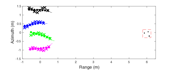
Figure 6: A distributed radar acquisition system with position ambiguity. The round dots indicate the assumed but erroneous antenna positions, while the $\times$’s indicate the true positions.

We generate ten different simulation layouts by randomly perturbing the positions of the antennas in the four arrays and constructing the five different target layouts shown in Figure 7. We compute the reconstructed images using the fused Lasso regularized least squares problem for both the ground truth and erroneous antenna positions. We also generate the imaging result from the measurement-domain blind deconvolution model in (6) by implementing a solver for a sparsity regularized version of the linear least squares problem of [38, 42]. Figure 7 shows the reconstructed images using the four methods above when the measurements are contaminated with 15dB PSNR noise. The figure illustrates that both the measurement-domain blind deconvolution method and our proposed image-domain blind deconvolution method are successful at recovering the target image. However, it can also be seen that our proposed method is much more robust to noise. For further validation, we present target detection receiver-operating-characteristic (ROC) curves in Figure 8 that demonstrate the superior performance of our method under the different noise levels.

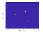
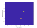
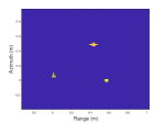
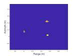
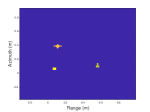
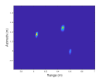
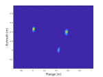
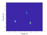
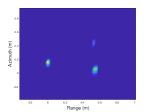
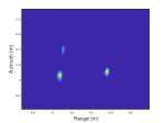
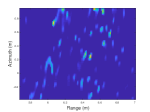
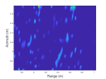
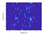
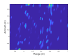
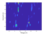
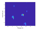
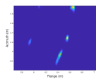
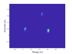
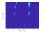
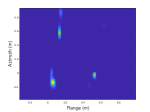
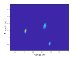
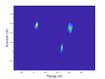
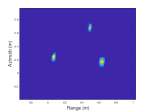
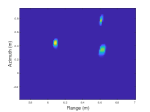
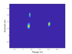
Figure 7: Ground truth and reconstructed images from noisy measurements at 15dB PSNR. First row shows an illustration of the five different target layouts used in our simulations. Second row uses fused Lasso reconstruction with the true antenna positions. Third row uses fused Lasso reconstruction with wrong antenna positions. Fourth row is the solution to the measurement-domain blind deconvolution problem. Last row is the solution of our proposed method for the image-domain blind deconvolution problem.

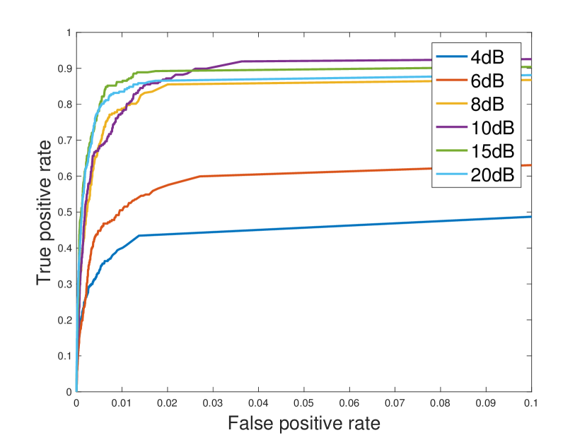
(a)

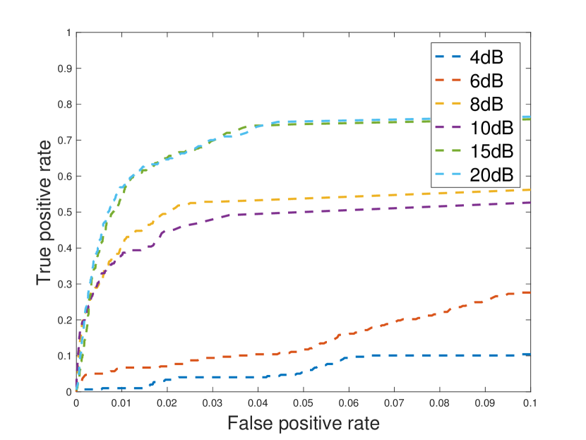
(b)

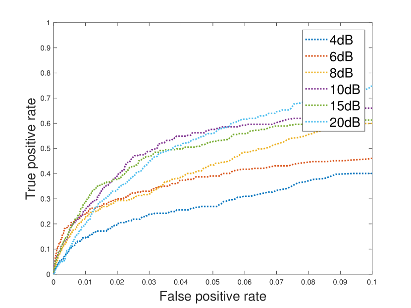
(c)

Figure 8: Target detection ROC curves of the reconstructed images using (a) the proposed method, (b) solving the measurement-domain blind deconvolution problem, and (c) fused Lasso recovery without compensating for position ambiguity.

Next, we compare the robustness of our proposed approach to the state of the art iterative perturbation estimation scheme of [17]. The method in [17] leverages the sparsity of the radar scene as well as the proximity between consecutive antenna positions in order to estimate the antenna perturbations and consequently improve the reconstructed image quality. Since the scheme in [17] relies on the antenna proximity to perform coherence analysis, we use additional measurements at antenna positions that interpolate the gaps between the $\times$’s for a total of 52 antenna positions per array. We compare the reconstruction performance in terms of the receiver operating characteristic (ROC) curves as shown in Figure 9. To generate the ROC curves, we simulate five different target positions as well as five different antenna perturbations and noise realizations. It can be seen from the figure that our proposed method is significantly more robust to measurement noise even at extreme noise levels. Finally, we recognize that the detection performance appears to be best for both methods at the 15dB PSNR level. We attribute this behavior to the limited number of noise realizations that have been used in our simulations which happened to be more favorable in the 15dB PSNR case.

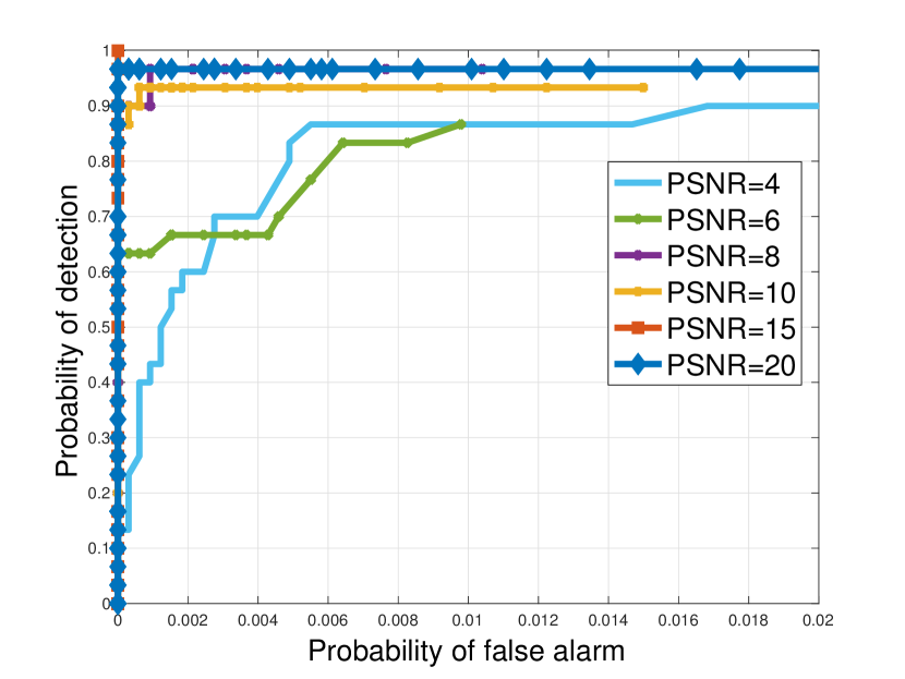
(a)

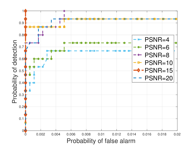
(b)

Figure 9: ROC curves of the reconstructed images using (a) our proposed sparse blind deconvolution scheme, and (b) the iterative perturbation estimation scheme of [17].

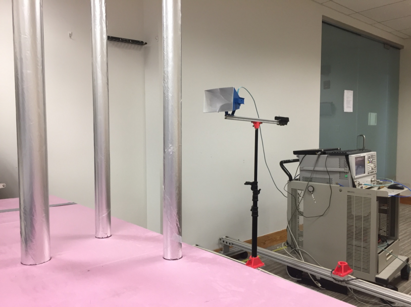
(a)

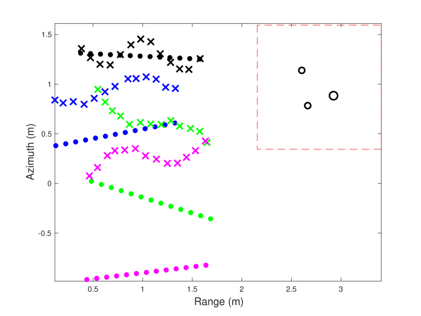
(b)

Figure 10: (a) Photograph of the horn antenna and three cylindrical targets used in our experimental setup. (b) Layout of the experimental distributed radar acquisition setup. The round dots indicate the assumed but erroneous antenna positions, while the $\times$’s indicate the true positions. The back circles in the top right corner indicate the target positions.

IV-B Experimental data

We built a radar setup using one horn antenna mounted on a platform that scans a scene that includes three cylindrical metal reflectors of diameter 6cm, 6cm, and 8.2 cm each, as shown in Figure 10 (a). The horn antenna was connected to a signal source, in this case an Agilent 2-Port PNA model 5230A, which measured the scattering parameters of the scene. The PNA was set to sweep over a frequency range from $1-10$ GHz with a 30 MHz frequency step and the port output power was set to 5 dBm. Over this range of frequencies the horn antennas have approximately a 40 degree main lobe beam width and a gain near 7 dBi. By moving the antenna positions and repeating the same experiment, we were able to collect radar measurements corresponding to four 13-element virtual arrays for a total of 52 antenna positions. A schematic of the experimental layout is shown in Figure 10 (b). The true antenna positions are indicated by the $\times$’s whereas the erroneous assumed positions are indicated by the dots. The horn of the antenna faces in the direction of the erroneous uniform linear array. With a 6 GHz center frequency and corresponding wavelength $\lambda_{c}=5$cm, the maximum position error was equal to $1.28\lambda_{c}$ in the horizontal (range) direction and $3.43\lambda_{c}$ in the vertical (azimuth) direction for array 1. On the other hand, the position error for arrays 2, 3, and 4 was over $10.8\lambda_{c}$ in the vertical direction. The target locations are indicated by the black circles inside the region of interest marked by the dashed red line.

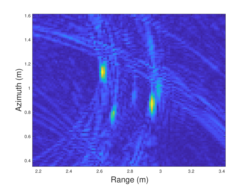
(a)

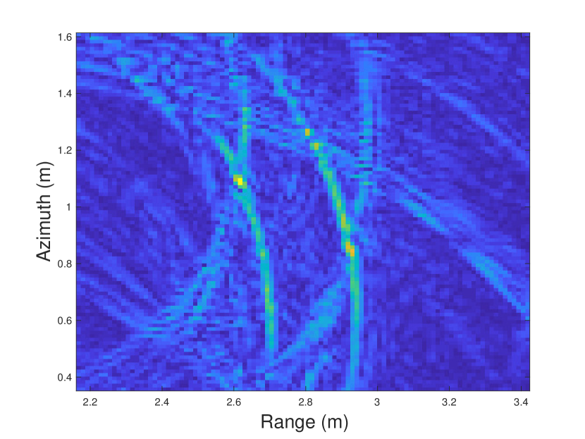
(b)

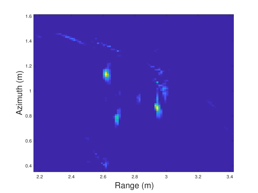
(c)

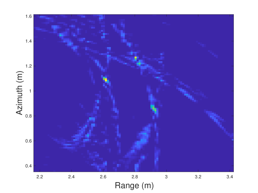
(d)

Figure 11: Imaging results for the experimental data obtained from applying backprojection using (a) the correct imaging operator corresponding to the true antenna positions, and (b) the wrong imaging operator corresponding to the erroneous uniformly spaced positions. Results obtained using fused Lasso regularized reconstruction with (c) the correct operator, and (d) the wrong operator.

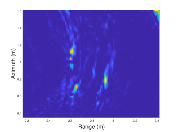
Figure 12: Reconstructed image from the experimental data using the proposed blind deconvolution approach.

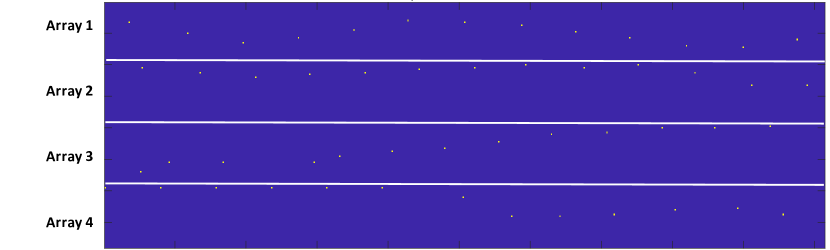
Figure 13: Recovered convolution filters using the proposed blind deconvolution autofocus algorithm.

We applied our blind deconvolution method to recover the radar image with parameters $\gamma=0.5$, $\mu=0.07$ and $\sigma=1.2$. The radar image is discretized into a $101\times 101$ image with pixel resolution equal to $\lambda_{c}/4=1.25$cm. We also set the size of the convolution filters equal to $39\times 39$ pixels which is larger than the perturbations of array 1 but smaller than the perturbation of arrays 2, 3, and 4. Figure 11 (a)–(d) shows the reconstructed images produced by the conventional backprojection scheme and a standard fused Lasso regularized reconstruction which do not compensate for the position ambiguity. Notice that when the wrong antenna positions are used to build the radar operator, the quality of the reconstructed imaged degrades significantly. On the other hand, our proposed framework is capable of generating a focused radar image in Figure 12 and compensates for the antenna perturbation by computing the spatial convolution filters shown in Figure 13. It is quite remarkable how the shift kernels for arrays 1 and 2 are consistent with the true antenna perturbations. The shift kernels of arrays 3 and 4 are only mildly following the antenna perturbation due to the large perturbation in the true antenna position compared to the erroneous assumed positions.

V Conclusion

We developed a novel image-domain blind deconvolution framework for recovering focused images from radar measurements that suffer from position ambiguity. Contrary to existing convex approaches to blind deconvolution, the proposed image-domain convolution model places the linear measurement operator after applying the convolution operation. We showed that this resulting model is exact in the setting when the transmitter and receiver antennas are affected by the same position error. To recover the scene, in the context of this framework, we also developed a block coordinate descent algorithm that alternates between recovering the target image under fused Lasso penalty constraints, and estimating the sparse convolution kernels of the antennas. The performance of the proposed formulation was shown to be superior to state-of-the-art methods that have addressed the radar autofocus problem. Future efforts will address deriving a convex formulation of the image-domain blind deconvolution problem.

References

- [1] H. Mansour, U. S. Kamilov, D. Liu, and P. T. Boufounos, “Radar autofocus using sparse blind deconvolution,” in IEEE International Conference on Acoustics, Speech and Signal Processing (ICASSP), April 2018, p. pp.
- [2] M. A. Herman and T. Strohmer, “High-resolution radar via compressed sensing,” IEEE Transactions on Signal Processing, vol. 57, no. 6, pp. 2275–2284, June 2009.
- [3] Y. Yu, A. P. Petropulu, and H. V. Poor, “Mimo radar using compressive sampling,” IEEE Journal of Selected Topics in Signal Processing, vol. 4, no. 1, pp. 146–163, Feb 2010.
- [4] C. R. Berger and J. M. F. Moura, “Noncoherent compressive sensing with application to distributed radar,” in 2011 45th Annual Conference on Information Sciences and Systems, March 2011, pp. 1–6.
- [5] D. Liu, U. S. Kamilov, and P. T. Boufounos, “Sparsity-driven distributed array imaging,” in 2015 IEEE 6th International Workshop on Computational Advances in Multi-Sensor Adaptive Processing (CAMSAP), Dec 2015, pp. 441–444.
- [6] L. Wang, B. Yazıci, and H. C. Yanik, “Antenna motion errors in bistatic SAR imagery,” Inverse Problems, vol. 31, no. 6, p. 065001, 2015. [Online]. Available: http://stacks.iop.org/0266-5611/31/i=6/a=065001
- [7] D. E. Wahl, P. H. Eichel, D. C. Ghiglia, and C. V. Jakowatz, “Phase gradient autofocus-a robust tool for high resolution SAR phase correction,” IEEE Transactions on Aerospace and Electronic Systems, vol. 30, no. 3, pp. 827–835, Jul 1994.
- [8] L. Xi, L. Guosui, and J. Ni, “Autofocusing of ISAR images based on entropy minimization,” IEEE Transactions on Aerospace and Electronic Systems, vol. 35, no. 4, pp. 1240–1252, Oct 1999.
- [9] W. Ye, T. S. Yeo, and Z. Bao, “Weighted least-squares estimation of phase errors for SAR/ISAR autofocus,” IEEE Transactions on Geoscience and Remote Sensing, vol. 37, no. 5, pp. 2487–2494, Sep 1999.
- [10] H. J. Cho and D. C. Munson, “Overcoming polar-format issues in multichannel SAR autofocus,” in 2008 42nd Asilomar Conference on Signals, Systems and Computers, Oct 2008, pp. 523–527.
- [11] K. H. Liu and D. C. Munson, “Fourier-domain multichannel autofocus for synthetic aperture radar,” IEEE Transactions on Image Processing, vol. 20, no. 12, pp. 3544–3552, Dec 2011.
- [12] M. P. Nguyen and S. B. Ammar, “Second order motion compensation for squinted spotlight synthetic aperture radar,” in Conference Proceedings of 2013 Asia-Pacific Conference on Synthetic Aperture Radar (APSAR), Sept 2013, pp. 202–205.
- [13] N. O. Onhon and M. Cetin, “A sparsity-driven approach for joint SAR imaging and phase error correction,” IEEE Transactions on Image Processing, vol. 21, no. 4, pp. 2075–2088, April 2012.
- [14] X. Du, C. Duan, and W. Hu, “Sparse representation based autofocusing technique for ISAR images,” IEEE Transactions on Geoscience and Remote Sensing, vol. 51, no. 3, pp. 1826–1835, March 2013.
- [15] S. Kelly, M. Yaghoobi, and M. Davies, “Sparsity-based autofocus for undersampled synthetic aperture radar,” IEEE Transactions on Aerospace and Electronic Systems, vol. 50, no. 2, pp. 972–986, April 2014.
- [16] J. Yang, X. Huang, J. Thompson, T. Jin, and Z. Zhou, “Compressed sensing radar imaging with compensation of observation position error,” IEEE Transactions on Geoscience and Remote Sensing, vol. 52, no. 8, pp. 4608–4620, Aug 2014.
- [17] D. Liu, U. S. Kamilov, and P. T. Boufounos, “Coherent distributed array imaging under unknown position perturbations,” in 4th International Workshop on Compressed Sensing Theory and its Applications to Radar, Sonar and Remote Sensing (CoSeRa), Sept 2016, pp. 105–109.
- [18] L. Zhao, L. Wang, G. Bi, S. Li, L. Yang, and H. Zhang, “Structured sparsity-driven autofocus algorithm for high-resolution radar imagery,” Signal Processing, vol. 125, pp. 376 – 388, 2016. [Online]. Available: http://www.sciencedirect.com/science/article/pii/S0165168416000426
- [19] M. J. Hasankhan, S. Samadi, and M. Çetin, “Sparse representation-based algorithm for joint SAR image formation and autofocus,” Signal, Image and Video Processing, vol. 11, no. 4, pp. 589–596, May 2017. [Online]. Available: https://doi.org/10.1007/s11760-016-0998-y
- [20] K. H. Liu, A. Wiesel, and D. C. Munson, “Synthetic aperture radar autofocus based on a bilinear model,” IEEE Transactions on Image Processing, vol. 21, no. 5, pp. 2735–2746, May 2012.
- [21] S. X. Zhang, M. D. Xing, X. G. Xia, Y. Y. Liu, R. Guo, and Z. Bao, “A robust channel-calibration algorithm for multi-channel in azimuth HRWS SAR imaging based on local maximum-likelihood weighted minimum entropy,” IEEE Transactions on Image Processing, vol. 22, no. 12, pp. 5294–5305, Dec 2013.
- [22] S. Ugur, O. Arıkan, and A. C. Gürbüz, “SAR image reconstruction by expectation maximization based matching pursuit,” Digital Signal Processing, vol. 37, pp. 75 – 84, 2015. [Online]. Available: http://www.sciencedirect.com/science/article/pii/S1051200414003182
- [23] A. Evers, N. Zimmerman, and J. A. Jackson, “Semidefinite relaxation autofocus for bistatic backprojection SAR,” in 2017 IEEE Radar Conference (RadarConf), May 2017, pp. 1332–1337.
- [24] R. L. Morrison, M. N. Do, and D. C. Munson, “SAR image autofocus by sharpness optimization: A theoretical study,” IEEE Transactions on Image Processing, vol. 16, no. 9, pp. 2309–2321, Sept 2007.
- [25] F. Berizzi, M. Martorella, A. Cacciamano, and A. Capria, “A contrast-based algorithm for synthetic range-profile motion compensation,” IEEE Transactions on Geoscience and Remote Sensing, vol. 46, no. 10, pp. 3053–3062, Oct 2008.
- [26] L. t. Zeng, Y. Liang, M. d. Xing, Z. y. Li, and Y. y. Huai, “Two-dimensional autofocus technique for high-resolution spotlight synthetic aperture radar,” IET Signal Processing, vol. 10, no. 6, pp. 699–707, 2016.
- [27] K. H. Liu, A. Wiesel, and D. C. Munson, “Synthetic aperture radar autofocus via semidefinite relaxation,” IEEE Transactions on Image Processing, vol. 22, no. 6, pp. 2317–2326, June 2013.
- [28] G. Xu, H. Liu, L. Tong, and T. Kailath, “A least-squares approach to blind channel identification,” IEEE Transactions on Signal Processing, vol. 43, no. 12, pp. 2982–2993, Dec 1995.
- [29] E. Moulines, P. Duhamel, J. F. Cardoso, and S. Mayrargue, “Subspace methods for the blind identification of multichannel fir filters,” IEEE Transactions on Signal Processing, vol. 43, no. 2, pp. 516–525, Feb 1995.
- [30] M. I. Gurelli and C. L. Nikias, “Evam: an eigenvector-based algorithm for multichannel blind deconvolution of input colored signals,” IEEE Transactions on Signal Processing, vol. 43, no. 1, pp. 134–149, Jan 1995.
- [31] K. Abed-Meraim, W. Qiu, and Y. Hua, “Blind system identification,” Proceedings of the IEEE, vol. 85, no. 8, pp. 1310–1322, Aug 1997.
- [32] L. Tong and S. Perreau, “Multichannel blind identification: from subspace to maximum likelihood methods,” Proceedings of the IEEE, vol. 86, no. 10, pp. 1951–1968, Oct 1998.
- [33] A. Ahmed, B. Recht, and J. Romberg, “Blind deconvolution using convex programming,” IEEE Transactions on Information Theory, vol. 60, no. 3, pp. 1711–1732, March 2014.
- [34] S. Ling and T. Strohmer, “Self-calibration and biconvex compressive sensing,” Inverse Problems, vol. 31, no. 11, p. 115002, 2015. [Online]. Available: http://stacks.iop.org/0266-5611/31/i=11/a=115002
- [35] Y. Li, K. Lee, and Y. Bresler, “Optimal sample complexity for blind gain and phase calibration,” IEEE Transactions on Signal Processing, vol. 64, no. 21, pp. 5549–5556, Nov 2016.
- [36] ——, “Identifiability in bilinear inverse problems with applications to subspace or sparsity-constrained blind gain and phase calibration,” IEEE Transactions on Information Theory, vol. 63, no. 2, pp. 822–842, Feb 2017.
- [37] A. Ahmed and L. Demanet, “Leveraging diversity and sparsity in blind deconvolution,” arXiv:1610.06098, 2016.
- [38] L. Balzano and R. Nowak, “Blind calibration of sensor networks,” in 2007 6th International Symposium on Information Processing in Sensor Networks, April 2007, pp. 79–88.
- [39] ——, Blind Calibration of Networks of Sensors: Theory and Algorithms. Boston, MA: Springer US, 2008, pp. 9–37. [Online]. Available: https://doi.org/10.1007/978-0-387-68845-9_1
- [40] R. Gribonval, G. Chardon, and L. Daudet, “Blind calibration for compressed sensing by convex optimization,” in 2012 IEEE International Conference on Acoustics, Speech and Signal Processing (ICASSP), March 2012, pp. 2713–2716.
- [41] Ç. Bilen, G. Puy, R. Gribonval, and L. Daudet, “Convex optimization approaches for blind sensor calibration using sparsity,” IEEE Transactions on Signal Processing, vol. 62, no. 18, pp. 4847–4856, Sept 2014.
- [42] S. Ling and T. Strohmer, “Self-calibration and bilinear inverse problems via linear least squares,” arXiv:1611.04196, 2016.
- [43] L. Wang and Y. Chi, “Blind deconvolution from multiple sparse inputs,” IEEE Signal Processing Letters, vol. 23, no. 10, pp. 1384–1388, Oct 2016.
- [44] X. Li, S. Ling, T. Strohmer, and K. Wei, “Rapid, robust, and reliable blind deconvolution via nonconvex optimization,” arXiv:1606.04933, 2016.
- [45] K. Lee, N. Tian, and J. Romberg, “Fast and guaranteed blind multichannel deconvolution under a bilinear system model,” arXiv:1610.06469, 2016.
- [46] V. Cambareri and L. Jacques, “A non-convex blind calibration method for randomised sensing strategies,” in 2016 4th International Workshop on Compressed Sensing Theory and its Applications to Radar, Sonar and Remote Sensing (CoSeRa), June 2016, pp. 16–20.
- [47] ——, “Through the haze: A non-convex approach to blind calibration for linear random sensing models,” arXiv:1610.09028, 2016.
- [48] D. Liu, G. Kang, L. Li, Y. Chen, S. Vasudevan, W. Joines, Q. H. Liu, J. Krolik, and L. Carin, “Electromagnetic time-reversal imaging of a target in a cluttered environment,” IEEE Transactions on Antennas and Propagation, vol. 53, no. 9, pp. 3058–3066, Sept 2005.
- [49] H. Mansour, U. Kamilov, D. Liu, P. Orlik, P. Boufounos, K. Parsons, and A. Vetro, “Online blind deconvolution for sequential through-the-wall-radar-imaging,” in 2016 4th International Workshop on Compressed Sensing Theory and its Applications to Radar, Sonar and Remote Sensing (CoSeRa), Sept 2016, pp. 61–65.
- [50] R. Tibshirani, M. Saunders, S. Rosset, J. Zhu, and K. Knight, “Sparsity and smoothness via the fused lasso,” Journal of the Royal Statistical Society: Series B (Statistical Methodology), vol. 67, no. 1, pp. 91–108, 2005. [Online]. Available: http://dx.doi.org/10.1111/j.1467-9868.2005.00490.x
- [51] A. Beck and M. Teboulle, “A fast iterative shrinkage-thresholding algorithm for linear inverse problems,” SIAM Journal on Imaging Sciences, vol. 2, no. 1, pp. 183–202, 2009. [Online]. Available: https://doi.org/10.1137/080716542
- [52] E. van den Berg and M. P. Friedlander, “Probing the pareto frontier for basis pursuit solutions,” SIAM Journal on Scientific Computing, vol. 31, no. 2, pp. 890–912, 2008. [Online]. Available: http://link.aip.org/link/?SCE/31/890
- [53] ——, “Sparse optimization with least-squares constraints,” SIAM J. Optimization, vol. 21, no. 4, pp. 1201–1229, 2011.
- [54] U. S. Kamilov, H. Mansour, and B. Wohlberg, “A plug-and-play priors approach for solving nonlinear imaging inverse problems,” IEEE Signal Processing Letters, vol. 24, no. 12, pp. 1872–1876, Dec 2017.
- [55] J. Douglas and H. H. Rachford, “On the numerical solution of heat conduction problems in two and three space variables,” Transaction of the American Mathematical Society, vol. 82, pp. 421–489, 1956.
- [56] S. Boyd, N. Parikh, E. Chu, B. Peleato, and J. Eckstein, “Distributed optimization and statistical learning via the alternating direction method of multipliers,” Found. Trends Mach. Learn., vol. 3, no. 1, pp. 1–122, Jan. 2011. [Online]. Available: http://dx.doi.org/10.1561/2200000016