A Fixed Mesh Method With Immersed Finite Elements
for Solving Interface Inverse Problems

Abstract

We present a new fixed mesh algorithm for solving a class of interface inverse problems for the typical elliptic interface problems. These interface inverse problems are formulated as shape optimization problems whose objective functionals depend on the shape of the interface. Regardless of the location of the interface, both the governing partial differential equations and the objective functional are discretized optimally, with respect to the involved polynomial space, by an immersed finite element (IFE) method on a fixed mesh. Furthermore, the formula for the gradient of the descritized objective function is derived within the IFE framework that can be computed accurately and efficiently through the discretized adjoint procedure. Features of this proposed IFE method based on a fixed mesh are demonstrated by its applications to three representative interface inverse problems: the interface inverse problem with an internal measurement on a sub-domain, a Dirichlet-Neumann type inverse problem whose data is given on the boundary, and a heat dissipation design problem.

Keywords: Inverse problems, Interface problems, Shape optimization, Discontinuous coefficients, Immersed finite element methods.

1 Introduction

In this article, we present a numerical method for solving a class of interface inverse problems with a fixed mesh by an immersed finite element (IFE) method. Without loss of generality, let $\Omega$ be a domain separated by an interface $\Gamma$ into two subdomains $\Omega^{-}$ and $\Omega^{+}$ each occupied by a different material represented by a piecewise constant function $\beta$ discontinuous across $\Gamma$. We consider a group of $K$ forward interface boundary problems posed on the domain $\Omega$ for the typical second order elliptic equation:

$$\begin{split}&-\nabla\cdot(\beta\nabla u^{k})=f^{k},~{}~{}\textrm{in}\;\Omega^{-}\cup\Omega^{+},\\ &u^{k}=g_{D}^{k},~{}~{}\textrm{on}\;\partial\Omega_{D}^{k}\subseteq\partial\Omega,~{}~{}\frac{\partial u^{k}}{\partial\mathbf{n}}=g_{N}^{k},~{}~{}\textrm{on}\;\partial\Omega_{N}^{k}\subseteq\partial\Omega,\end{split}~{}~{}~{}~{}~{}~{}\text{for~{}~{}}k=1,2,\cdots,K,$$ (1.1)

where $\overline{\partial\Omega_{N}^{k}}\cup\overline{\partial\Omega_{D}^{k}}=\partial\Omega$ and ${\bf n}$ is the outward normal of $\partial\Omega$, together with the jump conditions on the interface $\Gamma$:

$$\begin{split}&[u^{k}]|_{\Gamma}:=u^{k,+}-u^{k,-}=0,\\ &[\beta\nabla u^{k}\cdot\mathbf{n}]|_{\Gamma}:=\big{(}\beta^{+}\nabla u^{k,+}-\beta^{-}\nabla u^{k,-}\big{)}\cdot\mathbf{n}=0,\text{~{}~{}${\bf n}$ is the normal of $\Gamma$},\end{split}~{}~{}~{}~{}~{}~{}1\leq k\leq K,$$ (1.2)

$$\text{in which~{}~{}~{}}u^{k,s}=u^{k}|_{\Omega^{s}},~{}\beta(X)=\beta^{s}\text{~{}~{}for~{}~{}}X\in\Omega^{s},~{}s=-,+.$$ (1.3)

An important inverse problem related to the typical second order elliptic equation is to identify the coefficient $\beta$ where one needs to either identify the physical properties of materials, i.e., the values (the parameter estimation problem) and/or detect the location and shape of inclusions/interfaces (the inverse geometric problem) using the data measured for $u^{k},~{}1\leq k\leq K$ on a subset of the domain or on a subset of the boundary $\partial\Omega$ [20, 35, 40]. This type of inverse problems arise from many applications in engineering and sciences, such as the electrical impedance tomography (EIT) [12, 37] and groundwater or oil reservoir simulation [23, 73]. In the former case, $u^{k}$s and $\beta$ represent the electrical potential and the conductivity, respectively, whereas in the latter case $u^{k}$s and $\beta$ are the piezometric head and transmissivity, respectively. Similar inverse problems related to other partial differential equations also appear in applications, we refer readers to [36, 42] for medical imaging problems, [46, 68] for elasticity problems, and references therein. It is well known that these inverse problems are usually ill-posed especially when the available data is rather limited. Numerical methods based on the output-least-squares formulation are commonly used to handle these types of inverse problems, see [15, 18, 20, 35, 39] and references therein.

In many engineering and science applications, the values of material properties or parameters are known or chosen such as the elastic properties of tissue and bone in medical problems [55, 63] and the electrical properties in EIT problems [2, 8] to mention just a couple of applications. Thus, the focus of this article is to develop an efficient numerical method based on a fixed mesh for the inverse geometric problem related to the forward interface problem described by (LABEL:inter_prob_0) and (LABEL:jump_cond_0) in which we assume that the material values $\beta^{s}=\beta|_{\Omega^{s}},s=-,+$ are known priori and we need to use given measurements about $u$ to recover the location and geometry of the material interface $\Gamma$.

A widely used approach for an inverse geometric problem is the shape optimization method [32, 61] by which we seek for the interface $\Gamma^{*}$ from an optimization problem:

$$\Gamma^{*}=\textrm{argmin}\;\mathcal{J}(u^{1}(\Gamma),u^{1}(\Gamma),\cdots,u^{K}(\Gamma),\Gamma),$$ (1.4)

where

$$\mathcal{J}(u^{1}(\Gamma),u^{2}(\Gamma),\cdots,u^{K}(\Gamma),\Gamma)=\int_{\Omega_{0}}J(u^{1}(\Gamma),u^{2}(\Gamma),\cdots,u^{K}(\Gamma);X,\Gamma)dX,$$ (1.5)

and $u^{k}(\Gamma)$s are the solutions to the forward interface problems (LABEL:inter_prob_0) and (LABEL:jump_cond_0), but $\Omega_{0}\subseteq\Omega$ and
$J(u^{(1)}(\Gamma),u^{(2)}(\Gamma),\cdots,u^{(K)}(\Gamma);X,\Gamma)$ are application dependent, a few specific formulations of $J$ are given in Section 4 for a chosen group of representative applications. We note that the shape optimization approach has been applied to numerous applications, see for example [8, 11, 38, 47, 56].

The movement of the structure, boundary or interface is a critical issue in a shape optimization process challenging a solver chosen for the related forward problems. Traditional finite element methods can be used to obtain accurate solutions to the forward interface problems provided that they use a body fitting (or interface conforming) mesh [3, 14]; otherwise, their performance may not be satisfactory [6, 17]. The shape optimization methods based on body fitting mesh are referred as the Lagrangian approach [19] which, however, has a few drawbacks. The first concerns the mesh updating process from one iteration to the next in the optimization. As the geometry changes, to guarantee the accuracy, the mesh used by a chosen solver for the forward problem needs to be updated to fit the new shape of the boundary or interface [9, 70], which not only consumes time but also generates unsatisfactory meshes in many situations, see the illustrations in Figure 1.1 where the two plots on the left demonstrate an inappropriate mesh movement strategy leading to a mesh with less desirable qualities, especially near the right edge.

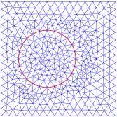
(a) The initial body fitting mesh

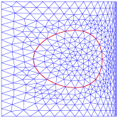
(b) The body fitting mesh after movement

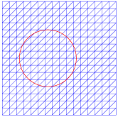
(c) The interface independent mesh

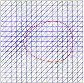
(d) The interface independent mesh

Figure 1.1: The body-fitting and interface independent mesh

The sensitivity analysis in a shape optimization is about the derivatives of an objective function with respect to the design variables, i.e., parameters describing the geometry of the domain [9, 32], and this leads to the gradient of the objective function which is a necessary ingredient in common numerical optimization algorithms such as descent direction methods and trust region methods [21, 59]. A velocity field defined as derivatives of node coordinates with respect to the design variables [19, 65] is usually employed in the sensitivity analysis. Several approaches for computing the velocity in a Lagrangian framework are summarized in [19], which either require computations to be carried out over the whole domain or need some special numerical methods for generating the velocity approximately.

Alternatively, the Eulerian approaches based on fixed meshes have been widely used in the shape optimization algorithms [43, 44], which allow the material interface/boundary to cut elements as illustrated in the two plots on the right in Figure 1.1. For example, the extended finite element methods (XFEM) based on a fixed mesh are used to solve optimal design problems problems [74, 69, 54, 57] and the inverse geometric problems related to crack detection [58, 64, 71]; the immersed interface methods (IIM) based on a Cartesian mesh is employed to solve an cavity (rigid inclusion) detection problem in [40]. Various techniques for improving the accuracy of the evaluation of either the stiffness matrix or sensitivity on those boundary/interface elements in Eulerian methods have been discussed in [4, 22, 41].

The goal of this article is to develop a fixed mesh method based on the partially penalized immersed finite element (PPIFE) method [51] for solving the inverse geometric problems/optimal design problems described by (LABEL:inter_prob_0)-(1.5). A key motivation is that IFE methods can solve interface forward problems with interface independent meshes optimally with respect to the degree of the involved polynomial spaces. In an IFE method, the interface shape/location and the jump conditions across the interface are utilized in the local IFE shape functions on interface elements, while the standard local finite element spaces are used on non-interface elements. Consequently, the convergence rates, optimal in the sense of the polynomials employed in the involved IFE spaces, have been established for IFE methods on interface independent meshes. We refer readers to IFE spaces constructed with linear polynomials [48, 49], with bilinear polynomial [33, 50], and with rotated-$Q_{1}$ polynomials [30, 75]. Applications of IFE methods to other types of equations or jump conditions can be found in [1, 34, 52, 16].

The advantages of the proposed IFE method for the inverse geometric problem are multifold. Because it is based on an interface independent fixed mesh in the shape optimization process, the issues caused by the mesh regeneration/movement, mesh distortion caused by large geometry changes, as well as some practical and theoretical issues for the construction of the velocity field [19] are circumvented, see the plots (c) and (d) in Figure 1.1 for an illustration. When the numerical interface curve $\Gamma$ is expressed as a parametric curve whose control points are the design variables for the shape optimization, the fixed mesh used in the proposed IFE method allows us to develop velocity fields and shape derivatives of IFE shape functions that are advantageous for efficient implementation because they all vanish outside interface elements whose total number is of the order $O(h^{-1})$ on a shape regular mesh compared to the total number of elements in the order of $O(h^{-2})$. In addition, the formulas for the velocity fields and shape derivatives in the propose IFE method can be implemented precisely without any further approximation procedures. Also, the IFE discretization for the related forward problem leads to an objective function that is optimal with respect to the polynomials employed in the underline finite element space regardless of the location of the interface to be optimized. Furthermore, using the IFE discretization we are able to derive formulas for the gradient with respect to the design variables for the objective function and these formulas can be efficiently executed within the IFE framework. These benefits together with the fact that no need to remesh again and again in the shape optimization demonstrate a very strong potential of the proposed IFE method.

This article is organized as follows. The next section recalls the linear IFE space and the related PPIFE scheme for the interface forward problems. Section 3 presents the shape optimization algorithm based on the IFE discretization on a fixed mesh of $\Omega$ for the inverse geometric problem described by (LABEL:inter_prob_0)-(1.5) and the computation procedure for its sensitivity. In Section 4, we demonstrate the strength and versatility of the proposed IFE method by applying it to three representative interface inverse problems.

2 An IFE Method for the Interface Forward Problems

In this section we recall the linear IFE method [29, 48] for the discretizatoin of the interface forward problem described by (LABEL:inter_prob_0) and (LABEL:jump_cond_0) with an interface independent mesh. The following notations will be used throughout this article. We let $\Gamma(t,{\boldsymbol{\alpha}}),t\in[0,1]$ be a parametrization of the interface $\Gamma$ with design variables as entries in the vector ${\boldsymbol{\alpha}}=(\alpha_{i})_{i\in\mathcal{D}}$ where $\mathcal{D}$ is the index set of the chosen design variables. For example, when $\Gamma(t,{\boldsymbol{\alpha}})$ is a cubic spline, ${\boldsymbol{\alpha}}$ is the vector of all the coordinates of control points [25]. Let $\mathcal{T}_{h}$ be an interface independent triangular mesh of the domain $\Omega$. An element $T\in\mathcal{T}_{h}$ will be called an interface element if its interior intersects the interface $\Gamma(t,{\boldsymbol{\alpha}})$; otherwise we call it a non-interface element. Let $\mathcal{T}^{i}_{h}$ ($\mathcal{E}^{i}_{h}$) and $\mathcal{T}^{n}_{h}$ ($\mathcal{E}^{n}_{h}$) be the sets of interface and non-interface elements (edges), respectively. Denote the set of the interior interface edges by $\mathring{\mathcal{E}}^{i}_{h}$. And let $\mathcal{N}_{h}=\{X_{1},X_{2},\cdots,X_{|\mathcal{N}_{h}|}\}$ and $\mathring{\mathcal{N}}_{h}$ be the sets of all the nodes in the mesh and the interior nodes, respectively.

For each element $T=\triangle A_{1}A_{2}A_{3}\in\mathcal{T}_{h}$, we let $\mathcal{I}=\{1,2,3\}$ and let $\psi^{non}_{i,T},i=1,2,3$ be the standard linear shape functions [10] such that $\psi^{non}_{i,T}(A_{j})=\delta_{ij},~{}i,j\in\mathcal{I}$. The local IFE space on each $T\in\mathcal{T}_{h}^{n}$ is

$$S_{h}(T)=\textrm{Span}\{\psi^{non}_{i,T},~{}i\in\mathcal{I}\}=\mathbb{P}_{1}.$$ (2.1)

On an interface element $T=\triangle A_{1}A_{2}A_{3}\in\mathcal{T}^{i}_{h}$, we let $P=(x_{P},y_{P})^{T}$ and $Q=(x_{Q},y_{Q})^{T}$ be the two interface-mesh intersection points, and let $l$ be the line connecting $P$ and $Q$. The normal vector for the line $l$ is $\bar{\mathbf{n}}=\frac{1}{||P-Q||}(y_{P}-y_{Q},-(x_{P}-x_{Q}))^{T}$ and the equation for the line $l$ is $L(X)=0$ with $L(X)=\bar{\mathbf{n}}\cdot(X-P).$ The line $l$ cuts the element into two sub-elements $\overline{T}^{+}$ and $\overline{T}^{-}$, see the sketch on the left in Figure 2.1, and we use them to introduce another two index sets $\mathcal{I}^{-}=\{i:A_{i}\in\overline{T}^{-}\}$ and $\mathcal{I}^{+}=\{i:A_{i}\in\overline{T}^{+}\}$.

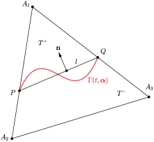
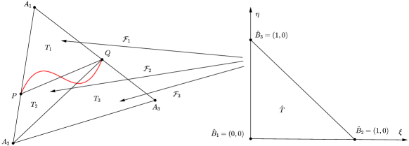
Figure 2.1: An interface element and its partitions.

According to [29], the linear IFE function constructed according to the interface jump condition (LABEL:jump_cond_0) and nodal values $\mathbf{v}=(v_{1},v_{2},v_{3})$ has the following formula

$$\psi^{int}_{T}(X)=\begin{cases}\psi^{int,-}_{T}(X)=\psi^{int,+}_{T}(X)+c_{0}L(X)&\text{if}\;\;X\in\overline{T}^{-},\\ \psi^{int,+}_{T}(X)=\sum_{i\in\mathcal{I}^{-}}c_{i}\psi^{non}_{i,T}(X)+\sum_{i\in\mathcal{I}^{+}}v_{i}\psi^{non}_{i,T}(X)&\text{if}\;\;X\in\overline{T}^{+},\end{cases}$$ (2.2)

with $$c_{0}=\left(\frac{\beta^{+}}{\beta^{-}}-1\right)\left(\sum_{i\in\mathcal{I}^{-}}c_{i}\nabla\psi^{non}_{i,T}\cdot\bar{\mathbf{n}}+\sum_{i\in\mathcal{I}^{+}}v_{i}\nabla\psi^{non}_{i,T}\cdot\bar{\mathbf{n}}\right),~{}~{}~{}~{}{\bf c}={\bf b}-\mu\frac{(\boldsymbol{\gamma}^{T}{\bf b})\boldsymbol{\delta}}{1+\mu\boldsymbol{\gamma}^{T}\boldsymbol{\delta}},$$ (2.3)

in which $$\boldsymbol{\gamma}=\left(\nabla\psi^{non}_{i,T}\cdot\bar{\mathbf{n}}\right)_{i\in\mathcal{I}^{-}},\boldsymbol{\delta}=\left(L(A_{i})\right)_{i\in\mathcal{I}^{-}},\;\;\;{\bf b}=\left(v_{i}-\mu L(A_{i})\sum_{j\in\mathcal{I}^{+}}\nabla\psi^{non}_{j,T}\cdot\bar{\mathbf{n}}~{}v_{j}\right)_{i\in\mathcal{I}^{-}}.$$ (2.4)

Then, using $\mathbf{v}=\mathbf{e}_{i},i\in\mathcal{I}$, the standard basis vectors of $\mathbb{R}^{3}$ in (2.2)-(2.4), we obtain the IFE shape functions $\psi^{int}_{i,T}(X),i\in\mathcal{I}$ satisfying $\psi^{int}_{i,T}(A_{j})=\delta_{ij}$ for $i,j\in\mathcal{I}$. The local IFE space on each $T\in\mathcal{T}_{h}^{i}$ is defined as

$$S_{h}(T)=\textrm{Span}\{\psi^{int}_{i,T}\,:\,i\in\mathcal{I}\}.$$ (2.5)

Local IFE spaces defined on all elements $\mathcal{T}_{h}$ are then used to define the IFE space globally as follows

$$S_{h}(\Omega)=\big{\{}v\in L^{2}(\Omega):v|_{T}\in S_{h}(T);v|_{T_{1}}(A)=v|_{T_{2}}(A),~{}\forall A\in\mathcal{N}_{h},\forall\,T_{1},T_{2}\in\mathcal{T}_{h}\text{~{}with~{}}A\in T_{1}\cap T_{2}\big{\}}.$$ (2.6)

With this IFE space and its associated space $S^{0}_{h}(\Omega)=\left\{v\in S_{h}(\Omega)~{}:~{}v(X)=0,~{}\forall X\in\mathcal{N}_{h}\cap\partial\Omega_{D}\right\}$, the interface forward problem (LABEL:inter_prob_0) and (LABEL:jump_cond_0) can be disretized by the symmetric PPIFE (SPPIFE) method [51] as follows: find $u_{h}^{k}\in S_{h}(\Omega),k=1,2,\cdots,K$ such that

$$\begin{split}&a_{h}(u_{h}^{k},v_{h})=L_{f}^{k}(v_{h}),~{}~{}~{}~{}\forall v_{h}\in S^{0}_{h}(\Omega),~{}~{}u_{h}^{k}(X)=g_{D}^{k}(X),~{}~{}~{}\forall X\in\mathcal{N}_{h}\cap\partial\Omega_{D}^{k},\end{split}$$ (2.7)

where the bilinear form $a_{h}$ and linear functional $L_{f}^{k}$ are given by

$$\begin{split}a_{h}(u_{h},v_{h})=&\sum_{T\in\mathcal{T}_{h}}\int_{T}\beta\nabla u_{h}\cdot\nabla v_{h}dX-\sum_{e\in\mathcal{E}^{i}_{h}\backslash\partial\Omega_{N}^{k}}\int_{e}\{\beta\nabla u_{h}\}_{e}\cdot[v_{h}]_{e}ds\\ &-\sum_{e\in\mathcal{E}^{i}_{h}\backslash\partial\Omega_{N}^{k}}\int_{e}\{\beta\nabla v_{h}\}_{e}\cdot[u_{h}]_{e}ds+\sum_{e\in\mathcal{E}^{i}_{h}}\frac{\sigma^{0}_{e}}{|e|}\int_{e}[u_{h}]_{e}\cdot[v_{h}]_{e}ds,~{}~{}\forall u_{h},v_{h}\in S_{h}(\Omega),\end{split}$$ (2.8)

$$\begin{split}L_{f}^{k}(v_{h})=&\int_{\Omega}f^{k}v_{h}dX+\int_{\partial\Omega_{N}^{k}}g_{N}^{k}v_{h}ds+\epsilon\sum_{e\in\mathcal{E}^{i}_{h}\cap\partial\Omega_{D}^{k}}\int_{e}\beta g_{D}^{k}\nabla v_{h}\cdot\mathbf{n}_{e}ds\\ &+\sum_{e\in\mathcal{E}^{i}_{h}\cap\partial\Omega_{D}^{k}}\frac{\sigma^{0}_{e}}{|e|}\int_{e}g_{D}^{k}v_{h}ds,~{}~{}\forall v_{h}\in S_{h}(\Omega).\end{split}$$ (2.9)

In the bilinear form $a_{h}(\cdot,\cdot)$, the operators $[\cdot]_{e}$ and $\{\cdot\}_{e}$ on each interior interface edge $e\in\mathring{\mathcal{E}}^{i}_{h}$ shared by $T_{1}$ and $T_{2}$ are such that $[v]_{e}=(v|_{T_{1}}\mathbf{n}^{1}_{e}+v|_{T_{2}}\mathbf{n}^{2}_{e})$, and $\{\beta\nabla v\}_{e}=\frac{1}{2}(\beta\nabla v|_{T_{1}}+\beta\nabla v|_{T_{2}}),~{}\forall v\in S_{h}(\Omega)$, where the normal vector $\mathbf{n}^{1}_{e}=-\mathbf{n}^{2}_{e}$ is from $T^{1}$ to $T^{2}$. For $e\in\mathcal{E}^{i}_{h}\cap\partial\Omega$, we define the operators $[\cdot]_{e}$ and $\{\cdot\}_{e}$ as $[v]_{e}=v|_{T}\mathbf{n}_{e},~{}\{\beta\nabla v\}_{e}=\beta\nabla v|_{T},~{}\forall v\in S_{h}(\Omega)$, where $T$ is the element that contains $e$ and $\mathbf{n}_{e}$ is the outward normal vector to $\partial\Omega$. In our applications, we choose $\sigma^{0}_{E}=10\max\{\beta^{-},\beta^{+}\}$. It has been proven [51] that the PPIFE solutions $u^{k}_{h}$ from (2.7) approximate the true solutions $u^{k}$, $1\leqslant k\leqslant K$, with an optimal accuracy with respect to the involved polynomials regardless of the interface location and shape, i.e.,

$$\|u^{k}_{h}-u^{k}\|_{L^{2}(\Omega)}+h|u^{k}_{h}-u^{k}|_{H^{1}(\Omega)}\leqslant Ch^{2}\|u\|_{H^{2}(\Omega)}.$$ (2.10)

We now put the SPPIFE method described by (2.7)-(2.9) in the matrix form. We assume that $S_{h}(\Omega)=\textrm{Span}\{\phi_{i}(X)~{}|~{}X_{i}\in\mathcal{N}_{h}\}$ in which $\phi_{i}(X)$ is the global IFE basis function associated with the node $X_{i}\in\mathcal{N}_{h}$. When the $k$-th ($1\leq k\leq K$) interface forward problem has a mixed boundary condition, we let $\mathcal{N}^{m}_{h}=\{X_{i}~{}|~{}X_{i}\in\mathring{\mathcal{N}}_{h}\cup\partial\Omega_{N}\}$ such that we can denote the SPPIFE solution $u_{h}^{k}(X)\in S_{h}(\Omega)$ determined by (2.7)-(2.9) as follows:

$$u_{h}^{k}(X)=\sum^{|\mathcal{N}^{m}_{h}|}_{i=1}u_{i}^{k}\phi_{i}(X)+\sum^{|\mathcal{N}_{h}|}_{i=|\mathcal{N}^{m}_{h}|+1}g_{D}^{k}(X_{i})\phi_{i}(X),$$ (2.11)

where, without loss of generality, we have assumed that nodes in $\mathcal{N}^{m}_{h}$ are ordered first. The stiffness matrix $\tilde{\mathbf{A}}=(a_{i,j})_{i,j=1}^{\left|\mathcal{N}_{h}\right|}$ associated with the bilinear form defined in (2.8) can be assembled from the following local matrices on elements and edges of $\mathcal{T}_{h}$:

$$\mathbf{K}_{T}=\left(\int_{T}\beta\nabla\psi_{p,T}\cdot\nabla\psi_{q,T}dX\right)_{p,q\in\mathcal{I}},~{}~{}~{}~{}~{}~{}~{}~{}~{}~{}~{}~{}~{}~{}~{}~{}~{}~{}~{}\forall T\in\mathcal{T}_{h},$$ (2.12a)

$$\mathbf{E}^{r_{1}r_{2}}_{e}=\left(\int_{e}\beta\nabla\psi_{p,T^{r_{1}}}\cdot(\psi_{q,T^{r_{2}}}\mathbf{n}^{r_{2}}_{e})ds\right)_{p,q\in\mathcal{I}},~{}~{}~{}~{}~{}~{}~{}~{}~{}~{}\forall e\in\mathcal{E}^{i}_{h},$$ (2.12b)

$$\mathbf{G}^{r_{1}r_{2}}_{e}=\left(\frac{\sigma^{0}_{e}}{|e|}\int_{e}(\psi_{p,T^{r_{1}}}\mathbf{n}^{r_{1}}_{e})\cdot(\psi_{q,T^{r_{2}}}\mathbf{n}^{r_{2}}_{e})ds\right)_{p,q\in\mathcal{I}},~{}~{}~{}~{}\forall e\in\mathcal{E}^{i}_{h},$$ (2.12c)

where the index $r_{1},r_{2}=1,2$ and the edge $e\in\mathring{\mathcal{E}}^{i}_{h}$ shared by the elements $T^{1}$ and $T^{2}$. But in the case $e\in\mathcal{E}^{i}_{h}\cap\partial\Omega$, we let $r_{1}=r_{2}=0$, $\mathbf{n}^{0}_{e}=\mathbf{n}_{e}$ is the outward normal vector and $T^{0}=T$ is the element that contains $e$. Let $\tilde{\mathbf{A}}_{b}^{m,k}=(a_{b,i}^{k})_{i=1}^{\left|\mathcal{N}_{h}\right|}=\tilde{\mathbf{A}}\begin{bmatrix}\bf{0}&\mathbf{g}_{D}^{k}\end{bmatrix}^{T},$ where $\bf{0}$ is the $\left|\mathcal{N}^{m}_{h}\right|$-dimensional zero vector and $\mathbf{g}_{D}^{k}=(g_{D}^{k}(X_{|\mathcal{N}^{m}_{h}|+1}),\cdots,g_{D}^{k}(X_{|\mathcal{N}_{h}|}))^{T}$. Similarly, the load vector $\tilde{\mathbf{F}}^{k}=(f_{i}^{k})_{i=1}^{\left|\mathcal{N}_{h}\right|}$ associated with the linear form defined in (2.9) can be assembled from the following vectors:

$$\mathbf{F}_{T}^{k}=\left(\int_{T}f^{k}\psi_{p,T}dX\right)_{p\in\mathcal{I}}, \forall T\in\mathcal{T}_{h},$$ (2.13a)

$$\mathbf{B}_{e}^{k}=\left(\int_{e}\beta g_{D}^{k}\nabla\psi_{p,T}\cdot\mathbf{n}_{e}ds\right)_{p\in\mathcal{I}},~{}~{}~{}\mathbf{C}_{e}^{k}=\frac{\sigma^{0}_{e}}{|e|}\left(\int_{e}\beta g_{D}^{k}\psi_{p,T}ds\right)_{p\in\mathcal{I}}, \forall e\in\mathcal{E}^{i}_{h}\cap\partial\Omega_{D},$$ (2.13b)

$$\mathbf{N}_{e}^{k}=\left(\int_{e}g_{N}^{k}\psi_{p,T}ds\right)_{p\in\mathcal{I}}, \forall e\in\mathcal{E}^{i}_{h}\cap\partial\Omega_{N}.$$ (2.13c)

Letting $\mathbf{u}_{h}^{m,k}=(u_{1}^{k},u_{2}^{k},\cdots,u_{|\mathcal{N}^{m}_{h}|}^{k})^{T}$, we can see that the unknown coefficient vector $\mathbf{u}_{h}^{m,k}$ of the SPPIFE solution $u_{h}^{k}(X)$ described by (2.11) is determined by the following linear system:

$$\mathbf{A}^{m,k}\mathbf{u}_{h}^{m,k}=\mathbf{F}^{m,k},$$ (2.14)

where $\mathbf{A}^{m,k}=(a_{i,j})_{i,j=1}^{\left|\mathcal{N}^{m}_{h}\right|}$, $\mathbf{F}^{m,k}=(f_{i}^{k})_{i=1}^{\left|\mathcal{N}^{m}_{h}\right|}-(a_{b,i}^{k})_{i=1}^{\left|\mathcal{N}^{m}_{h}\right|}$, and the superscript $m$ in (2.14) means that the boundary condition in the $k$-th interface forward problem is of a mixed type.

When the $k$-th ($1\leq k\leq K$) interface forward problem has Neumann boundary condition such that $\partial\Omega_{N}^{k}=\partial\Omega$, we know that $\left|\mathcal{N}_{h}^{m}\right|=\left|\mathcal{N}_{h}\right|$, $u_{h}^{k}(X)$ given in (2.11) does not have the second term and the related load vector $\tilde{\mathbf{F}}^{k}=(f_{i}^{k})_{i=1}^{\left|\mathcal{N}_{h}\right|}$ is assembled by the local vectors only in (2.13a) and (2.13c). Since the solution to the interface problem is not unique, as a common practice, the normalization condition $\int_{\Omega}u^{k}dX=u_{0}^{k}$ is imposed such that the SPPIFE solution $u_{h}^{k}(X)$ described by (2.11) is determined by the following linear system:

$$\mathbf{A}^{n}\mathbf{u}_{h}^{n,k}=\mathbf{F}^{n,k},~{}~{}~{}\text{with}~{}~{}\mathbf{A}^{n}=\begin{bmatrix}\tilde{\mathbf{A}}&\mathbf{R}\\ \mathbf{R}^{T}&0\end{bmatrix},~{}~{}\begin{cases}\mathbf{u}_{h}^{n,k}=[u_{1}^{k},u_{2}^{k},\cdots,u_{\left|\mathcal{N}_{h}\right|}^{k},\lambda]^{T},\\ \mathbf{F}^{n,k}=[f_{1}^{k},f_{2}^{k},\cdots,f_{\left|\mathcal{N}_{h}\right|}^{k},u_{0}^{k}]^{T},\end{cases}$$ (2.15)

where the superscript $n$ refers to a pure Neuman boundary condition, $\lambda$ is the Lagrange multiplier, and $\mathbf{R}$ is the vector assembled with the following local vector constructed on each element:

$$\mathbf{R}_{T}=\left(\int_{T}\psi_{p,T}dX\right)_{p\in\mathcal{I}},~{}~{}\forall T\in\mathcal{T}_{h}.$$ (2.16)

In summary, according to (2.14) and (2.15), the SPPIFE discretization for the $K$ interface forward problems described in (LABEL:inter_prob_0) and (LABEL:jump_cond_0) can be written in the following unified matrix form:

$$\mathbf{A}^{k}\mathbf{u}_{h}^{k}=\mathbf{F}^{k},~{}~{}\mathbf{u}_{h}^{k}=\begin{cases}\mathbf{u}_{h}^{m,k}\\ \mathbf{u}_{h}^{n,k}\end{cases}\mathbf{A}^{k}=\begin{cases}\mathbf{A}^{m}\\ \mathbf{A}^{n}\end{cases}\mathbf{F}^{k}=\begin{cases}\mathbf{F}^{m,k}&\text{for a mixed boundary condition},\\ \mathbf{F}^{n,k}&\text{for a Neumann boundary condition}.\end{cases}$$ (2.17)

We note that the matrices $\mathbf{A}^{k}$s in (2.17) are symmetric positive definite and their size and algebraic structure remain the same as the interface $\Gamma(t,{\boldsymbol{\alpha}}),t\in[0,1]$ evolves in a fixed mesh when the design variable ${\boldsymbol{\alpha}}$ varies.

3 An IFE Method for the Interface Inverse Problem

We now discuss the discretization of the inverse geometric problem (1.4) subject to the governing equations (LABEL:inter_prob_0) and (LABEL:jump_cond_0) by the SPPIFE method on a fixed mesh. When the design variable ${\boldsymbol{\alpha}}$ varies, the parametric interface $\Gamma=\Gamma(t,{\boldsymbol{\alpha}}),t\in[0,1]$ moves, and the two sub-domains $\Omega^{-}$ and $\Omega^{+}$ have to change their shapes correspondingly. Consequently, according to [19, 65], the spacial variables $X\in\Omega$ is considered as a mapping from the design variables ${\boldsymbol{\alpha}}$ to $\Omega$, i.e., $X=X({\boldsymbol{\alpha}})$, of which the derivative $\frac{\partial X}{\partial{\boldsymbol{\alpha}}}$ is the so called velocity field. This consideration implies that the local matrices (2.12a)-(2.12c), local vectors (2.13a)-(2.13c) and (2.16) should be influenced by this shape variation; hence, we write the matrix $\mathbf{A}^{k}$ and vector $\mathbf{F}^{k}$ in the SPPIFE equation (2.17) as $\mathbf{A}^{k}=\mathbf{A}^{k}(X({\boldsymbol{\alpha}}),{\boldsymbol{\alpha}}),~{}~{}\mathbf{F}^{k}=\mathbf{F}^{k}(X({\boldsymbol{\alpha}}),{\boldsymbol{\alpha}}),~{}~{}k=1,2,\cdots,K$, which further imply the solution ${\bf u}_{h}^{k}$ to the IFE equation (2.17) depends on $\alpha$ so we will denote it as ${\bf u}_{h}^{k}({\boldsymbol{\alpha}})$ from now on. Therefore, the IFE solution $u_{h}^{k}(X)$ to the $k$-th ($1\leq k\leq K$) governing interface forward problem in the form of (2.11) depends on ${\boldsymbol{\alpha}}$ through the IFE solution vector $\mathbf{u}_{h}^{k}({\boldsymbol{\alpha}})$, the spacial variable $X({\boldsymbol{\alpha}})$, and the IFE basis functions as follows

$$\begin{split}u_{h}^{k}(X)=u_{h}^{k}({\boldsymbol{\alpha}})=u_{h}^{k}(\mathbf{u}_{h}^{k}({\boldsymbol{\alpha}}),X({\boldsymbol{\alpha}}),{\boldsymbol{\alpha}})=&\sum^{|\mathcal{N}^{m}_{h}|}_{i=1}u_{i}^{k}({\boldsymbol{\alpha}})\phi_{i}(X({\boldsymbol{\alpha}}),{\boldsymbol{\alpha}})+\sum^{|\mathcal{N}_{h}|}_{i=|\mathcal{N}^{m}_{h}|+1}g_{D}^{k}(X_{i})\phi_{i}(X({\boldsymbol{\alpha}}),{\boldsymbol{\alpha}})\end{split}$$ (3.1)

where the second variable in $\phi_{i}(X({\boldsymbol{\alpha}}),{\boldsymbol{\alpha}})$ emphasizes the fact that ${\boldsymbol{\alpha}}$ also effects the IFE solution $u_{h}^{k}(X)$ through the coefficients of the IFE shape functions by the formulas (2.3)-(2.4).

The IFE solutions $u_{h}^{k}(X)\approx u^{k}(X),~{}1\leq k\leq K$ naturally suggest the following discretization of the integrand in the objective functional defined by (1.5):

$$J(u_{h}^{1}({\boldsymbol{\alpha}}),u_{h}^{2}({\boldsymbol{\alpha}}),\cdots,u_{h}^{K}({\boldsymbol{\alpha}});X,\Gamma(\cdot,{\boldsymbol{\alpha}}))\approx J(u^{1}({\boldsymbol{\alpha}}),u^{2}({\boldsymbol{\alpha}}),\cdots,u^{K}({\boldsymbol{\alpha}});X,\Gamma(\cdot,{\boldsymbol{\alpha}})).$$

Following explanations similar to those in the previous paragraph, the design variable ${\boldsymbol{\alpha}}$ can influence the approximate integrand $J(u_{h}^{1}({\boldsymbol{\alpha}}),u_{h}^{2}({\boldsymbol{\alpha}}),\cdots,u_{h}^{K}({\boldsymbol{\alpha}});X,\Gamma(\cdot,{\boldsymbol{\alpha}}))$ through $\mathbf{u}_{h}^{k}({\boldsymbol{\alpha}}),1\leq k\leq K$, $X({\boldsymbol{\alpha}})$, and ${\boldsymbol{\alpha}}$ itself; hence, we can denote these dependencies as

$$J_{h}(\mathbf{u}_{h}^{1}({\boldsymbol{\alpha}}),\mathbf{u}_{h}^{2}({\boldsymbol{\alpha}}),\cdots,\mathbf{u}_{h}^{K}({\boldsymbol{\alpha}}),X({\boldsymbol{\alpha}}),{\boldsymbol{\alpha}})\coloneqq J(u_{h}^{1}({\boldsymbol{\alpha}}),u_{h}^{2}({\boldsymbol{\alpha}}),\cdots,u_{h}^{K}({\boldsymbol{\alpha}});X,\Gamma(\cdot,{\boldsymbol{\alpha}})).$$ (3.2)

Therefore, we propose an IFE method for solving the inverse geometric problem described in (LABEL:inter_prob_0)-(1.5) on a fixed mesh of $\Omega$ by carrying out a shape optimization as follows: look for the design variable ${\boldsymbol{\alpha}}^{*}$ that can minimize the following objective function

$$\begin{split}&\mathcal{J}_{h}(\mathbf{u}_{h}^{1}({\boldsymbol{\alpha}}),\mathbf{u}_{h}^{2}({\boldsymbol{\alpha}}),\cdots,\mathbf{u}_{h}^{K}({\boldsymbol{\alpha}}),{\boldsymbol{\alpha}}):=\int_{\Omega_{0}}J_{h}(\mathbf{u}_{h}^{1}({\boldsymbol{\alpha}}),\mathbf{u}_{h}^{2}({\boldsymbol{\alpha}}),\cdots,\mathbf{u}_{h}^{K}({\boldsymbol{\alpha}}),X({\boldsymbol{\alpha}}),{\boldsymbol{\alpha}})dX,\\ \textrm{subject to}~{}~{}~{}~{}&\mathbf{A}^{k}(X({\boldsymbol{\alpha}}),{\boldsymbol{\alpha}})\mathbf{u}_{h}^{k}({\boldsymbol{\alpha}})-\mathbf{F}^{k}(X({\boldsymbol{\alpha}}),{\boldsymbol{\alpha}})=\mathbf{0},~{}~{}k=1,2,\cdots,K.\end{split}$$ (3.3)

The fact that the IFE solution $u_{h}^{k}(X),~{}1\leq k\leq K$ is an optimal approximation to $u^{k}(X),~{}1\leq k\leq K$ regardless of the location of the interface $\Gamma(t,{\boldsymbol{\alpha}}),~{}t\in[0,1]$ to be optimized in a chosen fixed mesh [51] implies that the objective function $\mathcal{J}_{h}(\mathbf{u}_{h}^{1}({\boldsymbol{\alpha}}),\mathbf{u}_{h}^{2}({\boldsymbol{\alpha}}),\cdots,\mathbf{u}_{h}^{K}({\boldsymbol{\alpha}}),{\boldsymbol{\alpha}})$ in this IFE method is an optimal approximation to the objective functional given in (1.5) regardless of the interface location in a chosen fixed mesh for common inverse geometric problems such as those to be presented in Section 4. For example, when the shape functional $J(u^{1},u^{2},\cdots,u^{K};X,\Gamma)$ is in the popular output-least-squares form such that:

$$J(u^{1},u^{2},\cdots,u^{K};X,\Gamma)=\sum_{k=1}^{K}|u^{k}-\bar{u}^{k}|^{2},$$ (3.4)

where $u^{1},u^{2},\cdots,u^{K}$ are the true solutions and $\bar{u}^{1},\bar{u}^{2},\cdots,\bar{u}^{K}$ are the given data functions in $L^{2}(\Omega)$, then, according to (3.2) and (LABEL:discrt_obj_2), we have

$$\begin{split}&\left|\mathcal{J}(u^{1},\cdots,u^{K},\Gamma)-\mathcal{J}_{h}({\bf u}_{h}^{1},\cdots,{\bf u}_{h}^{K},\Gamma)\right|\leqslant\int_{\Omega}|J(u^{1},\cdots,u^{K};X,\Gamma)-J(u^{1}_{h},\cdots,u^{K}_{h};X,\Gamma)|dX\\ =&\sum_{k=1}^{K}\int_{\Omega}|u^{k}-u^{k}_{h}|~{}|u^{k}+u^{k}_{h}-2\bar{u}^{k}|dX\\ \leqslant&\sum_{k=1}^{K}(\|u^{k}\|_{L^{2}(\Omega)}+\|u^{k}_{h}\|_{L^{2}(\Omega)}+2\|\bar{u}^{k}\|_{L^{2}(\Omega)})\|u^{k}-u^{k}_{h}\|_{L^{2}(\Omega)}\leqslant C(\|u^{k}\|^{2}_{H^{2}(\Omega)}+\|\bar{u}^{k}\|^{2}_{L^{2}(\Omega)})h^{2},\end{split}$$ (3.5)

where in the last step, we have applied the optimal estimation in the $L^{2}$ norm for the PPIFE solutions [51]: $\|u^{k}-u^{k}_{h}\|_{L^{2}(\Omega)}\leqslant Ch^{2}\|u^{k}\|_{H^{2}(\Omega)}$ which also implies $\|u^{k}_{h}\|\leqslant C\|u^{k}\|_{H^{2}(\Omega)}$. Therefore, it holds that

$$|\mathcal{J}(u^{1},u^{2},\cdots,u^{K},\Gamma)-\mathcal{J}_{h}({\bf u}_{h}^{1},{\bf u}_{h}^{2},\cdots,{\bf u}_{h}^{K},\Gamma)|\leqslant Ch^{2}$$ (3.6)

in which the constant $C$ depend on the solutions $u^{k}$ and data $\bar{u}^{k}$, $1\leqslant k\leqslant K$.

Furthermore, as discussed in the following subsections, we have formulas that can be efficiently executed in the IFE framework for accurately computing the gradient of this discrete objective function. These features are advantageous for implementing this IFE method with a typical numerical optimization algorithm, such as those based on the descent direction, for efficiently and accurately solving an inverse geometric problem described by (LABEL:inter_prob_0)-(1.5).

3.1 Velocity at Intersection Points

By (2.2), an IFE function on an interface element $T=\bigtriangleup A_{1}A_{2}A_{3}\in\mathcal{T}_{h}$ depends on the interface-mesh intersection points $P$ and $Q$, see the first sketch in Figure 2.1. Obviously, points $P$ and $Q$ change their locations when interface $\Gamma(t,{\boldsymbol{\alpha}}),~{}t\in[0,1]$ evolves due to the change in the design variables ${\boldsymbol{\alpha}}=(\alpha_{i})_{i\in\mathcal{D}}$. Hence, the objective function in (LABEL:discrt_obj_2) essentially depends on how the interface-mesh intersection points $P$ and $Q$ change when the design variable ${\boldsymbol{\alpha}}$ varies such that the derivatives of $P$ and $Q$ with respect to ${\boldsymbol{\alpha}}$ are critical ingredients for the sensitivity analysis of the proposed IFE method, and this motivates us to derive their formulas in this subsection. According to [57], these derivatives are the velocity defined at those intersection points and they will be used to develop the velocity field on the whole domain $\Omega$.

Assume that $\Gamma(t,{\boldsymbol{\alpha}})$ intersects with the edge of $T$ at points $P=(x_{P},y_{P})$ and $Q=(x_{Q},y_{Q})$ corresponding to certain parameters $\hat{t}_{P},\hat{t}_{Q}\in[0,1]$, see the illustration in Figure 2.1. Obviously, these two interface-mesh intersection points and their corresponding parameters $\hat{t}_{P}$ and $\hat{t}_{Q}$ all vary with respect to the design variable ${\boldsymbol{\alpha}}$; hence, we can express them as functions of ${\boldsymbol{\alpha}}$ as follows:

$$P=P({\boldsymbol{\alpha}})=(x_{P},y_{P})=(x(\hat{t}_{P}),y(\hat{t}_{P}))=(x(\hat{t}_{P}({\boldsymbol{\alpha}}),{\boldsymbol{\alpha}}),y(\hat{t}_{P}({\boldsymbol{\alpha}}),{\boldsymbol{\alpha}})),$$

$$Q=Q({\boldsymbol{\alpha}})=(x_{Q},y_{Q})=(x(\hat{t}_{Q}),y(\hat{t}_{Q}))=(x(\hat{t}_{Q}({\boldsymbol{\alpha}}),{\boldsymbol{\alpha}}),y(\hat{t}_{Q}({\boldsymbol{\alpha}}),{\boldsymbol{\alpha}})).$$

In the following discussions, we use $D_{\alpha_{j}}$ to denote the total derivative operator with respect to the $j$-th design variable $\alpha_{j}$, $j\in\mathcal{D}$, and $D_{{\boldsymbol{\alpha}}}$ is the corresponding gradient operator. But we use $\frac{\partial}{\partial\alpha_{j}}$ and $\frac{\partial}{\partial{\boldsymbol{\alpha}}}$ to denote the standard partial differential operators and the gradient operator with respect to $\alpha_{j}$ and ${\boldsymbol{\alpha}}$.

Without loss of generality, we assume that the interface-mesh intersection points are such that $P\in\overline{A_{1}A_{2}}$ and $Q\in\overline{A_{1}A_{3}}$ as illustrated in Figure 2.1. Then the following lemma establishes explicit formulas for computing the total derivatives of interface-mesh intersection points with respect to ${\boldsymbol{\alpha}}$.

Lemma 3.1.

Assume $\Gamma(t,{\boldsymbol{\alpha}})$ is not tangent to $A_{1}A_{2}$ at $P$. Then the function $P=P(\hat{t}_{P}({\boldsymbol{\alpha}}),{\boldsymbol{\alpha}})$ is differentiable and its velocity defined as the total derivatives $D_{\alpha_{j}}P$ with respect to $\alpha_{j}$, $j\in\mathcal{D}$ are determined by the following linear system:

$$M_{P}(\hat{t}_{P})~{}D_{\alpha_{j}}P=b_{P,j}(\hat{t}_{P}),~{}~{}\forall~{}j\in\mathcal{D},$$ (3.7)

with $$M_{P}(\hat{t}_{P})=\begin{bmatrix}y_{2}-y_{1}&-(x_{2}-x_{1})\\ \frac{\partial y}{\partial t}(\hat{t}_{P})&-\frac{\partial x}{\partial t}(\hat{t}_{P})\end{bmatrix}~{}~{}\textrm{and}~{}~{}b_{P,j}(\hat{t}_{P})=\begin{bmatrix}0\\ \frac{\partial y}{\partial t}(\hat{t}_{P})\frac{\partial x}{\partial\alpha_{j}}(\hat{t}_{P})-\frac{\partial x}{\partial t}(\hat{t}_{P})\frac{\partial y}{\partial\alpha_{j}}(\hat{t}_{P})\end{bmatrix}.$$

Proof.

First, differentiating $x_{P}=x(\hat{t}_{P}({\boldsymbol{\alpha}}),{\boldsymbol{\alpha}})$ and $y_{P}=y(\hat{t}_{P}({\boldsymbol{\alpha}}),{\boldsymbol{\alpha}})$ with respect to $\alpha_{j}$, we have $D_{\alpha_{j}}x_{P}=\frac{\partial x}{\partial t}\frac{\partial\hat{t}_{P}}{\partial\alpha_{j}}+\frac{\partial x}{\partial\alpha_{j}},~{}D_{\alpha_{j}}y_{P}=\frac{\partial y}{\partial t}\frac{\partial\hat{t}_{P}}{\partial\alpha_{j}}+\frac{\partial y}{\partial\alpha_{j}},$ which leads to

$$\frac{\partial y}{\partial t}D_{\alpha_{j}}x_{P}-\frac{\partial x}{\partial t}D_{\alpha_{j}}y_{P}=\frac{\partial y}{\partial t}\frac{\partial x}{\partial\alpha_{j}}-\frac{\partial x}{\partial t}\frac{\partial y}{\partial\alpha_{j}}.$$ (3.8)

On the other hand, since $P$ is on the edge $A_{1}A_{2}$, we have the equation $(y_{2}-y_{1})x_{P}-(x_{2}-x_{1})y_{P}=x_{2}y_{1}-x_{1}y_{2}.$ Differentiating it with respect to $\alpha_{j}$ yields

$$(y_{2}-y_{1})D_{\alpha_{j}}x_{P}-(x_{2}-x_{1})D_{\alpha_{j}}y_{P}=0.$$ (3.9)

Combining (3.9) and (3.8) yields the linear system for $D_{\alpha_{j}}P$ in (3.7). Let $\mathbf{n}_{e}$ be the normal vector to the edge $A_{1}A_{2}$. Then we have $\textrm{det}(M_{P}(\hat{t}_{P}))=\mathbf{n}_{e}\cdot\nabla\Gamma(\hat{t}_{P}({\boldsymbol{\alpha}}),{\boldsymbol{\alpha}})$ which is non zero by the assumption that $A_{1}A_{2}$ is not tangent to $\Gamma(t,{\boldsymbol{\alpha}})$ at $P$.

Similar results hold for the interface-mesh intersection point $Q$. Assume that $\Gamma(t,{\boldsymbol{\alpha}})$ is not tangent to $A_{1}A_{3}$ at $Q$, then the function $Q=Q(\hat{t}_{Q}({\boldsymbol{\alpha}}),{\boldsymbol{\alpha}})$ is differentiable and for $j\in\mathcal{D}$, $D_{\alpha_{j}}Q$ is determined by

$$M_{Q}(\hat{t}_{Q})~{}D_{\alpha_{j}}Q=b_{Q,j}(\hat{t}_{Q}),~{}~{}\forall~{}j\in\mathcal{D},$$ (3.10)

with $$M_{Q}(\hat{t}_{Q})=\begin{bmatrix}y_{3}-y_{1}&-(x_{3}-x_{1})\\ \frac{\partial y}{\partial t}(\hat{t}_{Q})&-\frac{\partial x}{\partial t}(\hat{t}_{Q})\end{bmatrix}~{}~{}~{}\textrm{and}~{}~{}~{}b_{Q,j}(\hat{t}_{Q})=\begin{bmatrix}0\\ \frac{\partial y}{\partial t}(\hat{t}_{Q})\frac{\partial x}{\partial\alpha_{j}}(\hat{t}_{Q})-\frac{\partial x}{\partial t}(\hat{t}_{Q})\frac{\partial y}{\partial\alpha_{j}}(\hat{t}_{Q})\end{bmatrix}.$$

Note that $\partial x/\partial t,\partial y/\partial t,\partial x/\partial\alpha_{j}$ and $\partial y/\partial\alpha_{j}$ required in formulas (3.7) and (3.10) depend on the chosen parametrization for the interface $\Gamma(t,{\boldsymbol{\alpha}})$, but they are usually easy to derive by standard calculus procedures.

Remark 3.1.

Let $\mathbf{n}_{e}$ be the normal of $\overline{A_{1}A_{2}}$, then we can directly verify that $D_{\alpha_{j}}P\cdot\mathbf{n}_{e}=\mathbf{n}_{e}M_{P}^{-1}b_{P}=0$ which means that $D_{\alpha_{j}}P$ is parallel to the edge $A_{1}A_{2}$ for any $\alpha_{j}$, $j\in\mathcal{D}$. Geometrically, this property implies that every intersection point can only move along the corresponding interface edge.

3.2 A Velocity Field for Sensitive Computations

In the inverse geometric problem, the two sub-domains $\Omega^{-}$ and $\Omega^{+}$ separated from each other by the interface $\Gamma=\Gamma(t,{\boldsymbol{\alpha}}),t\in[0,1]$ change their shapes when the parametric interface moves because of a variation in the design variable ${\boldsymbol{\alpha}}$. Hence, $\Omega^{-}$ and $\Omega^{+}$ can be considered as functions of ${\boldsymbol{\alpha}}$. Consequently, since $\Omega^{-}\cup\Omega^{+}=\Omega\backslash\Gamma$, we can consider the spacial variable $X\in\Omega$ as a mapping from the design variables ${\boldsymbol{\alpha}}$ to $\Omega$, i.e., $X=X({\boldsymbol{\alpha}})$, and its derivative $\frac{\partial X}{\partial{\boldsymbol{\alpha}}}$ is the so called velocity field [65], a key ingredient in the sensitivity analysis in shape optimizations. Therefore, in this subsection, we develop and analyze a velocity field for the IFE-based shape optimization to solve the inverse geometric problem.

Since the IFE method proposed in (LABEL:discrt_obj_2) is based on a fixed interface independent mesh, all the points located in non-interface elements can be considered as constant functions of the design variable ${\boldsymbol{\alpha}}$. Therefore, on such a fixed mesh used by the proposed IFE method, the velocity field vanish on all non-interface elements because $\frac{\partial X}{\partial{\boldsymbol{\alpha}}}=0$, and this suggests we need to discuss the velocity field only on interface elements.

As before, we consider a typical interface element $T=\bigtriangleup A_{1}A_{2}A_{3}\in\mathcal{T}_{h}^{i}$, without loss of generality, we assume that the parameterized interface $\Gamma(t,{\boldsymbol{\alpha}})=(x(t,{\boldsymbol{\alpha}}),y(t,{\boldsymbol{\alpha}})),~{}t\in[0,1]$ intersects with $T$ at $P({\boldsymbol{\alpha}})\in\overline{A_{1}A_{2}}$ and $Q({\boldsymbol{\alpha}})\in\overline{A_{1}A_{3}}$, see the first sketch in Figure 2.1, but neither $P$ nor $Q$ coincides with vertices of $T$. All results derived from now on are readily extended to the case in which one of the interface-mesh intersection points $P$ and $Q$ is a vertex of $T$.

Inspired by the ideas from [32, 57], we partition $T$ into three sub-elements as follows: $T_{1}=\bigtriangleup A_{1}PQ,~{}~{}T_{2}=\bigtriangleup A_{2}QP,~{}~{}T_{3}=\bigtriangleup A_{3}QA_{2},$ and let $\hat{T}=\bigtriangleup\hat{B}_{1}\hat{B}_{2}\hat{B}_{3}$ be the usual reference element with vertices $\hat{B}_{1}=(0,0)^{T},~{}~{}\hat{B}_{2}=(1,0)^{T},~{}~{}\hat{B}_{1}=(0,1)^{T},$ see the 2nd and the 3rd sketches in Figure 2.1. Then, the standard affine mappings from the reference element $\hat{T}=\bigtriangleup\hat{B}_{1}\hat{B}_{2}\hat{B}_{3}$ to $T_{m},m=1,2,3$ provide a relation between the points in $T$ and the design variable ${\boldsymbol{\alpha}}$ as follows:

$$X({\boldsymbol{\alpha}})=\mathcal{F}_{m}({\boldsymbol{\alpha}},\xi,\eta)=\mathbf{J}_{m}({\boldsymbol{\alpha}})\left(\begin{array}[]{c}\xi\\ \eta\end{array}\right)+A_{m},~{}~{}\text{for~{}~{}}\begin{pmatrix}\xi\\ \eta\end{pmatrix}\in\hat{T},~{}~{}m=1,2,3,$$ (3.11)

where the matrix $\mathbf{J}_{m}({\boldsymbol{\alpha}})$ is the Jacobian matrix of $\mathcal{F}_{m}$ such that $\mathbf{J}_{1}({\boldsymbol{\alpha}})=\left(P({\boldsymbol{\alpha}})-A_{1},Q({\boldsymbol{\alpha}})-A_{1}\right),~{}\mathbf{J}_{2}({\boldsymbol{\alpha}})=\left(Q({\boldsymbol{\alpha}})-A_{2},P({\boldsymbol{\alpha}})-A_{2}\right),~{}\mathbf{J}_{3}({\boldsymbol{\alpha}})=\left(Q({\boldsymbol{\alpha}})-A_{3},A_{2}-A_{3}\right).$ For every $X\in T$, the function $X({\boldsymbol{\alpha}})$ given in (3.11) is a piecewise differentiable function such that for every $j\in\mathcal{D}$

$$D_{\alpha_{j}}X({\boldsymbol{\alpha}})=(D_{\alpha_{j}}\mathbf{J}_{m}({\boldsymbol{\alpha}}))\mathbf{J}^{-1}_{m}({\boldsymbol{\alpha}})(X({\boldsymbol{\alpha}})-A_{m})~{}~{}~{}\text{for~{}}X({\boldsymbol{\alpha}})\in T_{m}\subseteq T,~{}m=1,2,3,$$ (3.12)

with $$D_{\alpha_{j}}\mathbf{J}_{1}({\boldsymbol{\alpha}})=\left(D_{\alpha_{j}}P,D_{\alpha_{j}}Q\right),~{}~{}D_{\alpha_{j}}\mathbf{J}_{2}({\boldsymbol{\alpha}})=\left(D_{\alpha_{j}}Q,D_{\alpha_{j}}P\right),~{}~{}D_{\alpha_{j}}\mathbf{J}_{3}({\boldsymbol{\alpha}})=\left(D_{\alpha_{j}}Q,\mathbf{0}\right),$$ (3.13)

in which $D_{\alpha_{j}}P$ and $D_{\alpha_{j}}Q$ are provided by the formulas (3.7) and (3.10). Therefore, by the formula for $X({\boldsymbol{\alpha}})\in T\in\mathcal{T}_{h}^{i}$ given in (3.11) and its derivatives given in (3.12), we introduce a piecewise velocity field $\mathbf{V}^{j}$ with respect to the $j$-th design variable $\alpha_{j}$, $j\in\mathcal{D}$ as follows:

$$\mathbf{V}^{j}(X)=\begin{cases}\mathbf{V}^{j}_{T}(X)=\mathbf{0},&\text{if $T\notin\mathcal{T}^{i}_{h}$ },\\ \mathbf{V}^{j}_{T}(X)=(D_{\alpha_{j}}\mathbf{J}_{m}({\boldsymbol{\alpha}}))\mathbf{J}^{-1}_{m}({\boldsymbol{\alpha}})(X({\boldsymbol{\alpha}})-A_{m}),&\text{if $T\in\mathcal{T}^{i}_{h}$ and $X\in T_{m}$},m=1,2,3.\end{cases}$$ (3.14)

We now present the properties of the velocity field by the following theorem.

Theorem 3.1.

For any $j\in\mathcal{D}$, the velocity $\mathbf{V}^{j}(X)$ defined in (3.14) has the properties:

• on each interface element $T=\bigtriangleup A_{1}A_{2}A_{3}\in\mathcal{T}_{h}^{i}$, there holds

  $$\mathbf{V}^{j}_{T}|_{A_{i}P}=\frac{\left\|X-A_{i}\right\|}{\left\|P-A_{i}\right\|}D_{\alpha_{j}}P,~{}i=1,2,~{}~{}~{} ~{}~{}~{}\mathbf{V}^{j}_{T}|_{A_{i}Q}=\frac{\left\|X-A_{i}\right\|}{\left\|Q-A_{i}\right\|}D_{\alpha_{j}}Q,~{}i=1,3,$$ (3.15a)

  $$\mathbf{V}^{j}_{T}|_{PQ}=\frac{\left\|X-Q\right\|}{\left\|P-Q\right\|}D_{\alpha_{j}}P+\frac{\left\|X-P\right\|}{\left\|P-Q\right\|}D_{\alpha_{j}}Q, ~{}~{}\mathbf{V}^{j}_{T}|_{A_{2}Q}=\frac{\left\|X-A_{2}\right\|}{\left\|Q-A_{2}\right\|}D_{\alpha_{j}}Q,~{}~{}\mathbf{V}^{j}_{T}|_{A_{2}A_{3}}=\mathbf{0},$$ (3.15b)

  $$\emph{div}(\mathbf{V}^{j}_{T_{m}})=\emph{tr}\left((D_{\alpha_{j}}\mathbf{J}_{m})\mathbf{J}^{-1}_{m}\right) ,~{}~{}m=1,2,3;$$ (3.15c)

• $\mathbf{V}^{j}\in H^{1}(\Omega)$ and $supp(\mathbf{V}^{j})\subseteq\bigcup_{T\in\mathcal{T}_{h}^{i}}T$;

• when restricted on each interface edge e, $\mathbf{V}^{j}(X)$ has the same direction as the edge e.

Proof.

P1 can be verified by calculation and the definition (3.14). P2 is the consequence of P1 and the definition (3.14). P3 is based on (3.15a) and Remark 3.1.

3.3 Shape Derivatives of IFE Shape Functions

In the proposed IFE method described by (LABEL:discrt_obj_2), the IFE basis functions $\phi_{i},1\leq i\leq\left|\mathcal{N}_{h}\right|$ on the chosen fixed interface independent mesh are directly employed in the objective function $\mathcal{J}_{h}$ according to (3.1) and (3.2). By their construction described in (2.2)-(2.4), the IFE basis functions change when the interface $\Gamma(t,{\boldsymbol{\alpha}}),t\in[0,1]$ moves because of the variations in the design variable ${\boldsymbol{\alpha}}$. Hence, the gradient of the objective function $\mathcal{J}_{h}$ in this IFE method inevitably involves the derivatives of the IFE basis functions with respect to ${\boldsymbol{\alpha}}$. By definition, each IFE basis function is a piecewise polynomial that is a linear combination of the IFE shape functions on each element described by (2.5) or (2.1) depending on whether the element is an interface element or not. Consequently, the derivative of an IFE basis function $\phi_{i}$ with respect to ${\boldsymbol{\alpha}}$ is zero on each non-interface element where all the shape functions are independent of ${\boldsymbol{\alpha}}$, and our focus in this subsection will be the derivative of IFE shape functions with respect to ${\boldsymbol{\alpha}}$ on interface elements. We note that [57, 74] presented similar approaches to calculate the shape derivative for special finite element shape functions.

Consider a typical interface element $T=\bigtriangleup A_{1}A_{2}A_{3}$ configured as in Figure 2.1. By (2.2) and the discussions at the beginning of this section and Section 3.1, we express an IFE shape function $\psi_{T}^{int}(X)$ on $T$ as $\psi_{T}^{int}(X)=\psi_{T}^{int}(X({\boldsymbol{\alpha}}),{\boldsymbol{\alpha}})$ to emphasize that the design variable ${\boldsymbol{\alpha}}$ influences the value of $\psi_{T}^{int}$ not only through the spatial variable $X$ which is a function of ${\boldsymbol{\alpha}}$ according to (3.11), but also directly through its coefficients $c_{0},{\bf c}$ and the coefficients of $L(X)$. However, the rate of change for an IFE shape function $\psi_{T}^{int}$ with respect to $\alpha_{j},j\in\mathcal{D}$ through $X({\boldsymbol{\alpha}})$ is readily known by the simple chain rule for differentiation because $\psi_{T}^{int}(X({\boldsymbol{\alpha}}),{\boldsymbol{\alpha}})$ depends on $X$ linearly and $\frac{\partial X}{\partial\alpha_{j}}$ is a velocity field already discussed in Section 3.2. Therefore, we only need to discuss the rate of change for an IFE shape function $\psi_{T}^{int}$ with respect to $\alpha_{j},j\in\mathcal{D}$ not through $X({\boldsymbol{\alpha}})$, and this rate of change is referred as a shape derivative in the shape optimization literature [32].

First, by their formulas given in Section 2, both $L(X)$ and $\bar{\mathbf{n}}$ depend on the design variable ${\boldsymbol{\alpha}}$ because of their dependence on the interface-mesh intersection points $P=(x_{P},y_{P})$ and $Q=(x_{Q},y_{Q})$ that are functions of ${\boldsymbol{\alpha}}$. By direct calculations, we have

$$\frac{\partial L}{\partial P}=\frac{(X-P)^{T}\bar{\mathbf{t}}\bar{\mathbf{n}}^{T}}{\left\|P-Q\right\|}+\bar{\mathbf{n}},~{}~{}\frac{\partial L}{\partial Q}=-\frac{(X-Q)^{T}\bar{\mathbf{t}}\bar{\mathbf{n}}^{T}}{\left\|P-Q\right\|},~{}~{}\frac{\partial\bar{\mathbf{n}}}{\partial P}=\frac{\bar{\mathbf{t}}\mathbf{\bar{n}}^{T}}{\left\|P-Q\right\|},~{}~{}\frac{\partial\bar{\mathbf{n}}}{\partial Q}=-\frac{\bar{\mathbf{t}}\mathbf{\bar{n}}^{T}}{\left\|P-Q\right\|},$$ (3.16)

where $\frac{\partial L}{\partial P}=(\frac{\partial L}{\partial x_{P}},\frac{\partial L}{\partial y_{P}})$, $\frac{\partial L}{\partial Q}=(\frac{\partial L}{\partial x_{Q}},\frac{\partial L}{\partial y_{Q}})$ are $1$-by-$2$ matrices, and $\bar{\mathbf{t}}=\frac{1}{\left\|P-Q\right\|}(x_{P}-x_{Q},y_{P}-y_{Q})^{T}$ is the tangential vector of $l$, $\frac{\partial\bar{\mathbf{n}}}{\partial P}=(\frac{\partial\bar{\mathbf{n}}}{\partial x_{P}},\frac{\partial\bar{\mathbf{n}}}{\partial y_{P}})$, $\frac{\partial\bar{\mathbf{n}}}{\partial Q}=(\frac{\partial\bar{\mathbf{n}}}{\partial x_{Q}},\frac{\partial\bar{\mathbf{n}}}{\partial y_{Q}})$ are $2$-by-$2$ matrices. Then, by the chain rule, we can use (3.16) to calculate $\frac{\partial L(X,{\boldsymbol{\alpha}})}{\partial\alpha_{j}}$ and $\frac{\partial\bar{\mathbf{n}}}{\partial\alpha_{j}}$ as follows:

$$\frac{\partial L(X,{\boldsymbol{\alpha}})}{\partial\alpha_{j}}=\frac{\partial L}{\partial P}~{}D_{\alpha_{j}}P+\frac{\partial L}{\partial Q}~{}D_{\alpha_{j}}Q,~{}~{}\frac{\partial\bar{\mathbf{n}}}{\partial\alpha_{j}}=\frac{\partial\bar{\mathbf{n}}}{\partial P}~{}D_{\alpha_{j}}P+\frac{\partial\bar{\mathbf{n}}}{\partial Q}~{}D_{\alpha_{j}}Q,$$ (3.17)

in which $D_{\alpha_{j}}P$ and $D_{\alpha_{j}}Q$ are given by formulas in (3.7), and (3.10).

Then, by (2.3) and (2.4), we have

$$\frac{\partial c_{0}}{\partial\alpha_{j}}=\mu\left(\sum_{i\in\mathcal{I}^{-}}\frac{\partial c_{i}}{\partial\alpha_{j}}\nabla\psi^{non}_{i,T}\cdot\bar{\mathbf{n}}+c_{i}\nabla\psi^{non}_{i,T}\cdot\frac{\partial\bar{\mathbf{n}}}{\partial\alpha_{j}}+\sum_{i\in\mathcal{I}^{+}}v_{i}\nabla\psi^{non}_{i,T}\cdot\frac{\partial\bar{\mathbf{n}}}{\partial\alpha_{j}}\right),$$ (3.18a)

$$\frac{\partial\boldsymbol{\gamma}}{\partial\alpha_{j}}=\left(\nabla\psi^{non}_{i,T}\cdot\frac{\partial\bar{\mathbf{n}}}{\partial\alpha_{j}}\right)_{i\in\mathcal{I}^{-}},\;\;\;\;\;\;\;\frac{\partial\boldsymbol{\delta}}{\partial\alpha_{j}}=\left(\frac{\partial L(A_{i})}{\partial\alpha_{j}}\right)_{i\in\mathcal{I}^{-}},$$ (3.18b)

$$\frac{\partial{\bf b}}{\partial\alpha_{j}}=\left(-\mu\frac{\partial L(A_{i})}{\partial\alpha_{j}}\sum_{j\in\mathcal{I}^{+}}\nabla\psi^{non}_{j,T}\cdot\bar{\mathbf{n}}~{}v_{j}-\mu L(A_{i})\sum_{j\in\mathcal{I}^{+}}\nabla\psi^{non}_{j,T}\cdot\frac{\partial\bar{\mathbf{n}}}{\partial\alpha_{j}}~{}v_{j}\right)_{i\in\mathcal{I}^{-}}.$$ (3.18c)

Furthermore, by (2.3) again, we can compute $\frac{\partial\mathbf{c}}{\partial\alpha_{j}},j\in\mathcal{D}$ from (3.18b), (3.18c) as follows:

$$\frac{\partial\mathbf{c}}{\partial\alpha_{j}}=\frac{\partial\mathbf{b}}{\partial\alpha_{j}}-\mu\frac{\left[\left(\frac{\partial\boldsymbol{\gamma}}{\partial\alpha_{j}}\right)^{T}\mathbf{b}\boldsymbol{\delta}+\boldsymbol{\gamma}^{T}\frac{\partial\mathbf{b}}{\partial\alpha_{j}}\boldsymbol{\delta}+\boldsymbol{\gamma}^{T}\mathbf{b}\frac{\partial\boldsymbol{\delta}}{\partial\alpha_{j}}\right](1+\mu\boldsymbol{\gamma}^{T}\boldsymbol{\delta})-\mu\boldsymbol{\gamma}^{T}\mathbf{b}\boldsymbol{\delta}\left[\left(\frac{\partial\boldsymbol{\gamma}}{\partial\alpha_{j}}\right)^{T}\boldsymbol{\delta}+\boldsymbol{\gamma}^{T}\frac{\partial\boldsymbol{\delta}}{\partial\alpha_{j}}\right]}{(1+\mu\boldsymbol{\gamma}^{T}\boldsymbol{\delta})^{2}}.$$ (3.19)

Finally, we use (3.17), (3.18a), and (3.19) to obtain the formula for the shape derivatives of an IFE shape function defined by (2.2) by the following formula: for every $j\in\mathcal{D}$,

$$\frac{\partial\psi^{int}_{T}(X,{\boldsymbol{\alpha}})}{\partial\alpha_{j}}=\begin{cases}\frac{\textstyle\partial\psi^{int,-}_{T}(X,{\boldsymbol{\alpha}})}{\textstyle\partial\alpha_{j}}=\frac{\textstyle\partial\psi^{int,+}_{T}(X,{\boldsymbol{\alpha}})}{\textstyle\partial\alpha_{j}}+\frac{\textstyle\partial c_{0}}{\textstyle\partial\alpha_{j}}L(X,{\boldsymbol{\alpha}})+c_{0}\frac{\textstyle L(X,{\boldsymbol{\alpha}})}{\textstyle\partial\alpha_{j}}&\text{if}\;\;X\in\overline{T}^{-},\\ \\ \frac{\textstyle\partial\psi^{int,+}_{T}(X,{\boldsymbol{\alpha}})}{\textstyle\partial\alpha_{j}}=\sum_{i\in\mathcal{I}^{-}}\frac{\textstyle\partial c_{i}}{\textstyle\partial\alpha_{j}}\psi^{non}_{i,T}(X)&\text{if}\;\;X\in\overline{T}^{+}.\end{cases}$$ (3.20)

3.4 The Gradient of the Discretized Objective Function

The gradient of the objective function $\mathcal{J}_{h}$ is necessary for implementing the proposed IFE method with a common minimization algorithm based on a decent direction or trust region. We now put all the preparations in the previous subsections together to derive the formula for the gradient of the objective function $\mathcal{J}_{h}$ that can be executed efficiently within the IFE framework. This formula involves the total derivatives of $\mathcal{J}_{h}$ with respect to ${\boldsymbol{\alpha}}_{j},~{}j\in\mathcal{D}$ depending on the velocity field and these total derivatives are also referred as the material derivatives of $\mathcal{J}_{h}$ in the shape optimization literature [32]. For the simplicity of presentation, we assume that the boundary condition functions $g^{k}_{N}$, $g^{k}_{D}$ and the force term $f^{k}$ are fixed and independent with interface change, $1\leqslant k\leqslant K$. In the following this discussion, we use $\nabla$ to denote the standard gradient operator with respect to $X$. We start from the material derivatives with respect to $\alpha_{j},j\in\mathcal{D}$ of the local matrices and vectors which are used to construct $\mathbf{A}^{k}(X({\boldsymbol{\alpha}}),{\boldsymbol{\alpha}})$ and $\mathbf{F}^{k}(X({\boldsymbol{\alpha}}),{\boldsymbol{\alpha}})$. Their formulas are presented in the two theorems below, of which the derivation is based on Lemma 3.3 of [32] in the direction of the velocity field developed in Section 3.2 together with the properties in Theorem 3.1 and the shape derivatives of the IFE shape functions given by the formula (3.20)

Theorem 3.2.

On each interface element $T\in\mathcal{T}_{h}^{i}$ and each interface edge $e\in\mathcal{E}_{h}^{i}$, we have the following formulas for the material derivatives of $\mathbf{K}_{T},\mathbf{E}_{e}^{r_{1},r_{2}},\mathbf{G}_{e}^{r_{1},r_{2}}$ and $\mathbf{R}_{T}$ with respect to $\alpha_{j},j\in\mathcal{D}$:

$$D_{\alpha_{j}}\mathbf{K}_{T} =\left(\int_{T}\beta\nabla\frac{\partial\psi_{p,T}}{\partial\alpha_{j}}\cdot\nabla\psi_{q,T}dX\right)_{p,q\in\mathcal{I}}+\left(\int_{T}\beta\nabla\frac{\partial\psi_{p,T}}{\partial\alpha_{j}}\cdot\nabla\psi_{q,T}dX\right)_{p,q\in\mathcal{I}}^{T}$$

$$~{}~{}~{}~{}~{}~{}+\left(\sum_{i=1}^{3}\int_{T_{i}}\beta\nabla\psi_{p,T}\cdot\nabla\psi_{q,T}~{}dX~{}\emph{tr}\left((D_{\alpha_{j}}\mathbf{J}_{i})\mathbf{J}^{-1}_{i}\right)\right)_{p,q\in\mathcal{I}},$$ (3.21a)

$$D_{\alpha_{j}}\mathbf{E}^{r_{1}r_{2}}_{e} =\left(\int_{e}\beta\nabla\frac{\partial\psi_{p,T^{r_{1}}}}{\partial\alpha_{j}}\cdot(\psi_{q,T^{r_{2}}}\mathbf{n}^{r_{2}}_{e})ds\right)_{p,q\in\mathcal{I}}+\left(\int_{e}\beta\nabla\psi_{p,T^{r_{1}}}\cdot(\frac{\partial\psi_{q,T^{r_{2}}}}{\partial\alpha_{j}}\mathbf{n}^{r_{2}}_{e})ds\right)_{p,q\in\mathcal{I}}$$

$$~{}~{}+\Bigg{(}\beta^{-}\nabla\psi^{-}_{p,T^{r_{1}}}\cdot(\psi^{-}_{q,T^{r_{2}}}\mathbf{n}^{r_{2}}_{e})|_{P}-\beta^{+}\nabla\psi^{+}_{p,T^{r_{1}}}\cdot(\psi^{+}_{q,T^{r_{2}}}\mathbf{n}^{r_{2}}_{e})|_{P}\Bigg{)}_{p,q\in\mathcal{I}}\frac{D_{\alpha_{j}}P\cdot(A_{2}-A_{1})}{\left\|A_{2}-A_{1}\right\|},$$ (3.21b)

$$D_{\alpha_{j}}\mathbf{G}^{r_{1}r_{2}}_{e} =\frac{\sigma^{0}_{e}}{|e|}\left(\int_{e}(\frac{\partial\psi_{p,T^{r_{1}}}}{\partial\alpha_{j}}\mathbf{n}^{r_{1}}_{e})\cdot(\psi_{q,T^{r_{2}}}\mathbf{n}^{r_{2}}_{e})ds+\int_{e}(\psi_{p,T^{r_{1}}}\mathbf{n}^{r_{1}}_{e})\cdot(\frac{\partial\psi_{q,T^{r_{2}}}}{\partial\alpha_{j}}\mathbf{n}^{r_{2}}_{e})ds\right)_{p,q\in\mathcal{I}},$$ (3.21c)

$$D_{\alpha_{j}}\mathbf{R}_{T} =\left(\int_{T}\frac{\partial\psi_{p,T}}{\partial\alpha_{j}}dX+\int_{T}\nabla\psi_{p,T}\cdot\mathbf{V}^{j}dX\right)_{p\in\mathcal{I}}+\left(\sum_{i=1}^{3}\int_{T_{i}}\psi_{p,T}~{}dX~{}\emph{tr}\left((D_{\alpha_{j}}\mathbf{J}_{i})\mathbf{J}^{-1}_{i}\right)\right)_{p\in\mathcal{I}}.$$ (3.21d)

Theorem 3.3.

On each interface element $T\in\mathcal{T}_{h}^{i}$ and each interface edge $e\in\mathcal{E}_{h}^{i}$, we have the following formulas for the material derivatives of $\mathbf{F}_{T},\mathbf{B}_{e},\mathbf{C}_{e}$ and $\mathbf{N}_{e}$ with respect to $\alpha_{j},j\in\mathcal{D}$:

$$D_{\alpha_{j}}\mathbf{F}_{T}^{k} =\left(\int_{T}f^{k}\frac{\partial\psi_{p,T}}{\partial\alpha_{j}}dX\right)_{p\in\mathcal{I}}+\left(\int_{T}\nabla(f^{k}\psi_{p,T})\cdot\mathbf{V}^{j}_{T}dX\right)_{p\in\mathcal{I}}$$

$$+\left(\sum_{i=1}^{3}\int_{T_{i}}f^{k}\psi_{p,T}~{}dX~{}\emph{tr}\left((D_{\alpha_{j}}\mathbf{J}_{i})\mathbf{J}^{-1}_{i}\right)\right)_{p\in\mathcal{I}},$$ (3.22a)

$$D_{\partial_{j}}\mathbf{B}_{e}^{k} =\left(\int_{e}\beta g_{D}^{k}\nabla\frac{\partial\psi_{p,T}}{\partial\alpha_{j}}\cdot\mathbf{n}_{e}ds\right)_{p\in\mathcal{I}}$$

$$~{}~{}~{}~{}~{}~{}~{}~{}+\Bigg{(}\beta^{-}g_{D}^{k}\nabla\psi^{-}_{p,T}\cdot\mathbf{n}_{e}|_{P}-\beta^{+}g_{D}^{k}\nabla\psi^{+}_{p,T}\cdot\mathbf{n}_{e}|_{P}\Bigg{)}_{p\in\mathcal{I}}\frac{D_{\alpha_{j}}P\cdot(A_{2}-A_{1})}{\left\|A_{2}-A_{1}\right\|},$$ (3.22b)

$$D_{\partial_{j}}\mathbf{C}_{e}^{k} =\frac{\sigma^{0}_{e}}{|e|}\left(\int_{e}\beta g_{D}^{k}\frac{\partial\psi_{p,T}}{\partial\alpha_{j}}ds\right)_{p\in\mathcal{I}}+\frac{\sigma^{0}_{e}}{|e|}\Bigg{(}\beta^{-}g_{D}^{k}\psi^{-}_{p,T}|_{P}-\beta^{+}g_{D}^{k}\psi^{+}_{p,T}|_{P}\Bigg{)}_{p\in\mathcal{I}}\frac{D_{\alpha_{j}}P\cdot(A_{2}-A_{1})}{\left\|A_{2}-A_{1}\right\|},$$ (3.22c)

$$D_{\partial_{j}}\mathbf{N}_{e}^{k} =\left(\int_{e}g_{N}^{k}\frac{\partial\psi_{p,T}}{\partial\alpha_{j}}ds\right)_{p\in\mathcal{I}}+\Bigg{(}g_{N}^{k}\psi^{-}_{p,T}|_{P}-g_{N}^{k}\psi^{+}_{p,T}|_{P}\Bigg{)}_{p\in\mathcal{I}}\frac{D_{\alpha_{j}}P\cdot(A_{2}-A_{1})}{\left\|A_{2}-A_{1}\right\|}.$$ (3.22d)

Now, by Lemma 3.3 in [32] again, we have the following standard formula for the material derivative associated to the $j$-th design variable $\alpha_{j}$:

$$D_{\alpha_{j}}\mathcal{J}_{h}=\sum_{k=1}^{K}\left(\frac{\partial\mathcal{J}_{h}}{\partial\mathbf{u}_{h}^{k}}\cdot D_{\alpha_{j}}\mathbf{u}_{h}^{k}\right)+\int_{\Omega_{0}}\frac{\partial J_{h}}{\partial\alpha_{j}}dX+\int_{\Omega_{0}}\nabla J_{h}\cdot\mathbf{V}^{j}dX+\int_{\Omega_{0}}J_{h}~{}\textrm{div}\left(\mathbf{V}^{j}\right)dX$$ (3.23)

in which we have used the fact that $\frac{\partial\mathcal{J}_{h}}{\partial\mathbf{u}_{h}^{k}}=\int_{\Omega_{0}}\frac{\partial J_{h}}{\partial\mathbf{u}_{h}^{k}}dX$, and, as demonstrated by examples presented in the next section, $\frac{\partial\mathcal{J}_{h}}{\partial\mathbf{u}_{h}^{k}},\nabla J_{h},\frac{\partial J_{h}}{\partial\alpha_{j}}$ and $J_{h}$ itself are problem dependent, but they are usually easy to calculate for many applications. Also, we note that $\mathbf{V}^{j}$ is given in (3.14) and $\textrm{div}\left(\mathbf{V}^{j}\right)$ is given in (3.15c); hence, we proceed to derive formula for $\left(\frac{\partial\mathcal{J}_{h}}{\partial\mathbf{u}_{h}^{k}}\right)\cdot D_{\alpha_{j}}\mathbf{u}_{h},~{}j\in\mathcal{D}$ which can be directly used in (3.23).

For $D_{\alpha_{j}}\mathbf{u}_{h}^{k},1\leq k\leq K,j\in\mathcal{D}$, by differentiating the IFE system in (2.17) with respect to $\alpha_{j}$, we have the following linear system for $D_{\alpha_{j}}\mathbf{u}_{h}^{k}$: $\mathbf{A}^{k}(X({\boldsymbol{\alpha}}),{\boldsymbol{\alpha}})~{}D_{\alpha_{j}}\mathbf{u}_{h}^{k}=D_{\alpha_{j}}\mathbf{F}^{k}(X({\boldsymbol{\alpha}}),{\boldsymbol{\alpha}})-D_{\alpha_{j}}\mathbf{A}^{k}(X({\boldsymbol{\alpha}}),{\boldsymbol{\alpha}})~{}\mathbf{u}_{h}^{k}({\boldsymbol{\alpha}})$, $1\leq k\leq K.$ Then, by the standard process in the discretized adjoint method [27], we can compute $\left(\frac{\partial\mathcal{J}_{h}}{\partial\mathbf{u}_{h}^{k}}\right)\cdot D_{\alpha_{j}}\mathbf{u}_{h}^{k}$ efficiently (especially when $\left|\mathcal{D}\right|$ is large) by solving for $\mathbf{Y^{k}}$ from $\big{(}\mathbf{A}^{k}\big{)}^{T}\mathbf{Y}^{k}=\frac{\partial\mathcal{J}_{h}}{\partial\mathbf{u}_{h}^{k}}$, and then

$$\begin{split}\left(\frac{\partial\mathcal{J}_{h}}{\partial\mathbf{u}_{h}^{k}}\right)\cdot D_{\alpha_{j}}\mathbf{u}_{h}&=\mathbf{Y}^{k}\cdot\left(D_{\alpha_{j}}\mathbf{F}^{k}(X({\boldsymbol{\alpha}}),{\boldsymbol{\alpha}})-D_{\alpha_{j}}\mathbf{A}^{k}(X({\boldsymbol{\alpha}}),{\boldsymbol{\alpha}})~{}\mathbf{u}_{h}^{k}({\boldsymbol{\alpha}})\right),~{}~{}1\leq k\leq K,\end{split}$$ (3.24)

where $\mathbf{A}^{k}$ is the matrix for the $k$-th IFE equation described in (2.17). As summarized in the next section, one advantage of the proposed IFE method is that computations for the material derivatives (3.23) can be very efficiently implemented in the IFE framework.

3.5 Implementation

In this subsection, we discuss the implementation of the proposed IFE-based shape optimization method. First, we summarize the discretization of forward/inverse problems and the sensitivity computation discussed in the previous subsections into the following algorithm.

Algorithm The IFE Shape Optimization Algorithm

1:Generate a fixed mesh and choose an initial design variable ${\boldsymbol{\alpha}}$.

2:Loop until convergence.

3:Prepare data:

4:a: use the design variables to generate the parametric curve as the numerical interface;

5:b: find the interface-mesh intersection points, interface edges and interface elements.

6:Prepare matrices and vectors for the IFE systems and compute the cost function:

7:a: use (2.12) and (2.13) and the IFE shape functions given in (2.1) and (2.5) to assemble matrices and vectors $\mathbf{A}^{k},\mathbf{F}^{k},1\leq k\leq K$ for the IFE systems (2.17);

8:b: compute the PPIFE solutions $\mathbf{u^{k}},1\leq k\leq K$ by (2.17) and compute the objective function $\mathcal{J}_{h}(\mathbf{u}_{h}^{1}({\boldsymbol{\alpha}}),\mathbf{u}_{h}^{2}({\boldsymbol{\alpha}}),\cdots,\mathbf{u}_{h}^{K}({\boldsymbol{\alpha}}),{\boldsymbol{\alpha}})$ in (LABEL:discrt_obj_2).

9:Compute the shape sensitivities:

10:a: prepare the velocity fields $\mathbf{V}^{j}$, $j\in\mathcal{D}$, and shape derivatives of IFE shape functions according to (3.14) and (3.20), respectively;

11:b: form the material derivatives of local matrices and vectors according to Theorem 3.2 and Theorem 3.3, and use them to assemble the global matrices $D_{\alpha_{j}}\mathbf{A}^{k}(X({\boldsymbol{\alpha}}),{\boldsymbol{\alpha}})$ and vectors $D_{\alpha_{j}}\mathbf{F}^{k}(X({\boldsymbol{\alpha}}),{\boldsymbol{\alpha}})$;

12:c: compute $\frac{\partial\mathcal{J}_{h}}{\partial\mathbf{u}_{h}^{k}}\cdot D_{\alpha_{j}}\mathbf{u}_{h}^{k}$ for $k=1,\cdots,K$, according to (3.24);

13:d: compute the terms $\int_{\Omega_{0}}\frac{\partial J_{h}}{\partial\alpha_{j}}dX$, $\int_{\Omega_{0}}\nabla J_{h}\cdot\mathbf{V}^{j}dX$ and $\int_{\Omega_{0}}J_{h}\text{div}(\mathbf{V}^{j})dX$ according to the given shape functional;

14:e: compute the material derivatives of the objective function according to (3.23).

15:Update the design variable ${\boldsymbol{\alpha}}$ by a chosen gradient-based optimization algorithm.

16:End loop

In this proposed IFE Shape Optimization Algorithm, we note that the mesh is fixed during the optimization process, and the only mesh information needed to be updated are those interface-mesh intersection points and interface elements/edges. Consequently, the global matrices $\mathbf{A}^{k}$ and vectors $\mathbf{F}^{k}$ in step 4 remain the same size and algebraic structure on this fixed mesh, which is beneficial for implementation. Also, they do not need to be completely re-assembled in each iteration, because only those global basis functions whose supports overlap with the interface elements/edges in two consecutive iterations are changed. As a result, their assemblage can be done very efficiently by just updating those entries corresponding to the global basis functions whose supports overlap with the interface elements/edges in the previous and the current iteration.

In step 5 above (computing the shape sensitivities), we emphasize that the velocity fields and the shape derivatives of IFE shape functions are only needed on interface elements, which can be implemented according to the analytical formulas (3.14) and (3.20). These two quantities vanishing over all the non-interface elements make the whole procedure of shape sensitivity computation remarkably efficient. Firstly the integration of the terms $\int_{\Omega_{0}}\nabla J_{h}\cdot\mathbf{V}^{j}dX$ and $\int_{\Omega_{0}}J_{h}\text{div}(\mathbf{V}^{j})dX$ in the material derivative of the objective functional (3.23) only needs to be done on interface elements intersecting $\Omega_{0}$ because the involved integrands all vanish on the non-interface elements. Secondly assembling the matrices $D_{\alpha_{j}}\mathbf{F}^{k}(X({\boldsymbol{\alpha}}),{\boldsymbol{\alpha}})$ and $D_{\alpha_{j}}\mathbf{A}^{k}(X({\boldsymbol{\alpha}}),{\boldsymbol{\alpha}})$, i.e., the material derivatives of global matrices $\mathbf{A}^{k}$ and $\mathbf{F}^{k}$, is also a very efficient process since it is only performed over the interface elements/edges by the explicit formulas given in Theorems 3.2 and 3.3. In summary, the shape sensitivity in this algorithm is done by computations only need to be carried out over interface elements whose number is in the order of $O(h^{-1})$ versus the number of all elements in the order of $O(h^{-2})$ in the mesh. In contrast, preparing $D_{\alpha_{j}}\mathbf{F}^{k}(X({\boldsymbol{\alpha}}),{\boldsymbol{\alpha}})$ and $D_{\alpha_{j}}\mathbf{A}^{k}(X({\boldsymbol{\alpha}}),{\boldsymbol{\alpha}})$ is usually expensive within the Lagrange framework where a global velocity field requires to carry out the assemblages over all elements in a mesh [19], and $D_{\alpha_{j}}\mathbf{F}^{k}(X({\boldsymbol{\alpha}}),{\boldsymbol{\alpha}})$ and $D_{\alpha_{j}}\mathbf{A}^{k}(X({\boldsymbol{\alpha}}),{\boldsymbol{\alpha}})$ are usually prepared approximately in methods in the Eullerian framework, see related discussions in [22, 72, 74].

In addition, whenever necessary, one could refine the mesh easily at any point of the optimization process. Because of the Cartesian grid used by the IFE method, information in the previous mesh can be easily transformed to a new mesh through an interpolation operator. As demonstrated by examples presented in the last section, we note that the mesh refinement actually enables us to obtain better reconstruction of interface in some challenging inverse geometric problems.

Finally, we note that the proposed IFE shape optimization algorithm is highly parallelizable because computing the velocity fields $\mathbf{V}^{j}$ (3.14), shape derivatives of IFE shape functions $\frac{\partial\phi_{T}}{\partial\alpha_{j}}$ (3.20) and the material derivatives of stiffness matrices and vectors $D_{\alpha_{j}}\mathbf{A}^{k}(X({\boldsymbol{\alpha}}),{\boldsymbol{\alpha}})$ and $D_{\alpha_{j}}\mathbf{F}^{k}(X({\boldsymbol{\alpha}}),{\boldsymbol{\alpha}})$, i.e., the material derivatives of objective functions (3.23) with respect to each individual design variable $\alpha_{j}$, are independent with each other. Hence these computations can be done very efficiently with an easy implementation on modern parallel computers.

Therefore, we believe these properties together with the optimal accuracy of PPIFE solutions (2.10) and the resulted optimal accuracy of discretized objective functions, regardless of the interface location, make the proposed IFE shape optimization algorithm advantageous compared with those in the literature.

4 Some Applications

In this section, we demonstrate how the general IFE method proposed in the previous section can use a fixed mesh to solve a wide spectrum of interface inverse problems posed in the format of (LABEL:inter_prob_0)-(1.5) by applying this method to, but not limited to, three representative interface inverse/design problems: (1). the output-least-squares problem [13, 15, 28]; (2). the Dirichlet-Neumann problem [8, 37, 67]; and (3). the heat dissipation minimization problem [24, 47, 76]. The first problem uses the interior data available on the whole or a portion of $\Omega$ to reconstruct/design the interface, the second one recovers the interface from the data only available on $\partial\Omega$, and the last one is an application for optimal design of heat conduction fields. These examples also provide additional hints/suggestions about how to implement the proposed IFE method efficiently.

All numerical examples to be presented are posed on the domain $\Omega=(-1,1)\times(-1,1)$ on which Cartesian meshes for these numerical examples are formed by cutting $\Omega$ into $N\times N$ congruent small squares and then cutting each small square into two triangles along a diagonal line of this small square. In the following discussion, we will specify the mesh size $N$ for each example and the numerical interface curve is parameterized by a cubic spline. This choice of parametrization is based on the accuracy, versatility, and popularity of the cubic spline, and we emphasize that the fixed mesh method developed here can be readily extended to other parameterizations.

4.1 An Output-Least-Squares Problem

In this example, we consider an interface inverse/design problem associated to the interface forward problem described by (LABEL:inter_prob_0) and (LABEL:jump_cond_0) with $K=1$, in which, we assume an observation data $\bar{u}$ for the solution $u^{1}$ to the forward problem (or a target function in optimal design application) is available on a sub-domain $\Omega_{0}\subseteq\Omega$, and we need to recover/design the location and the shape of the interface from $\bar{u}$ by solving an output-least-squares problem [15, 40], i.e., by optimizing the following shape functional

$$\mathcal{J}(u^{1}(\Gamma),\Gamma)=\int_{\Omega_{0}}(u^{1}-\bar{u})^{2}dx$$ (4.1)

where $u^{1}$ is the solution to the interface forward problem described by (LABEL:inter_prob_0), (LABEL:jump_cond_0) and (1.3) with a pure Dirichlet boundary condition $g^{1}_{D}$ on the whole $\partial\Omega$. This problem appears in oil/underwater reservoirs [23, 73] and optimal designing of cooling elements in battery systems [62]. And a related time dependent problem is discussed in [31]. Applying the IFE method proposed in (LABEL:discrt_obj_2) to the inverse problem formulated in (4.1) suggests to seek the design variable ${\boldsymbol{\alpha}}^{*}$ that minimizes the following discrete objective functional

$$\begin{split}&\mathcal{J}_{h}({\bf u}_{h}^{1}({\boldsymbol{\alpha}}),{\boldsymbol{\alpha}})=\int_{\Omega_{0}}J_{h}({\bf u}_{h}^{1}({\boldsymbol{\alpha}}),X({\boldsymbol{\alpha}}),{\boldsymbol{\alpha}})dX,\\ \text{subject to}~{}~{}~{}~{}~{}~{}&\mathbf{A}^{1}(X({\boldsymbol{\alpha}}),{\boldsymbol{\alpha}}){\bf u}_{h}^{1}(\alpha)-{\bf F}^{1}(X({\boldsymbol{\alpha}}),{\boldsymbol{\alpha}})=\mathbf{0},\end{split}$$ (4.2)

where, expressing the IFE solution $u_{h}^{1}({\boldsymbol{\alpha}})=u_{h}^{1}(\mathbf{u}_{h}^{1}({\boldsymbol{\alpha}}),X({\boldsymbol{\alpha}}),{\boldsymbol{\alpha}})$ in the format given in (3.1), we have

$$\begin{split}J_{h}({\bf u}_{h}^{1}({\boldsymbol{\alpha}}),X({\boldsymbol{\alpha}}),{\boldsymbol{\alpha}})&=\big{(}{\tilde{J}}_{h}({\bf u}_{h}^{1}({\boldsymbol{\alpha}}),X({\boldsymbol{\alpha}}),{\boldsymbol{\alpha}})\big{)}^{2},\\ \text{with~{}~{}}{\tilde{J}}_{h}({\bf u}_{h}^{1}({\boldsymbol{\alpha}}),X({\boldsymbol{\alpha}}),{\boldsymbol{\alpha}})&=\sum^{|\mathring{\mathcal{N}}_{h}|}_{i=1}u_{i}^{1}({\boldsymbol{\alpha}})\phi_{i}(X({\boldsymbol{\alpha}}),{\boldsymbol{\alpha}})+\sum^{|\mathcal{N}_{h}|}_{i=|\mathring{\mathcal{N}}_{h}|+1}g^{1}_{D}(X_{i})\phi_{i}(X({\boldsymbol{\alpha}}),{\boldsymbol{\alpha}})-\bar{u}.\\ \end{split}$$ (4.3)

We have shown in (3.6) that this discretized objective function has the optimal second order accuracy to approximate the continuous one regardless of the interface location and shape. According to (4.3), the evaluation of $J_{h}({\bf u}_{h}^{1}({\boldsymbol{\alpha}}),X({\boldsymbol{\alpha}}),{\boldsymbol{\alpha}})$ is straightforward and it is obvious that

$$\begin{split}&\nabla J_{h}=2{\tilde{J}}_{h}({\bf u}_{h}^{1}({\boldsymbol{\alpha}}),X({\boldsymbol{\alpha}}),{\boldsymbol{\alpha}})\left(\sum^{|\mathring{\mathcal{N}}_{h}|}_{i=1}u_{i}^{1}({\boldsymbol{\alpha}})\nabla\phi_{i}(X({\boldsymbol{\alpha}}),{\boldsymbol{\alpha}})+\sum^{|\mathcal{N}_{h}|}_{i=|\mathring{\mathcal{N}}_{h}|+1}g^{1}_{D}(X_{i})\nabla\phi_{i}(X({\boldsymbol{\alpha}}),{\boldsymbol{\alpha}})-\nabla\bar{u}\right),\\ &\frac{\partial J_{h}}{\partial\alpha_{j}}=2{\tilde{J}}_{h}({\bf u}_{h}^{1}({\boldsymbol{\alpha}}),X({\boldsymbol{\alpha}}),{\boldsymbol{\alpha}})\left(\sum^{|\mathring{\mathcal{N}}_{h}|}_{i=1}u_{i}^{1}({\boldsymbol{\alpha}})\frac{\partial\phi_{i}(X({\boldsymbol{\alpha}}),{\boldsymbol{\alpha}})}{\partial\alpha_{j}}+\sum^{|\mathcal{N}_{h}|}_{i=|\mathring{\mathcal{N}}_{h}|+1}g^{1}_{D}(X_{i})\frac{\partial\phi_{i}(X({\boldsymbol{\alpha}}),{\boldsymbol{\alpha}})}{\partial\alpha_{j}}\right),\end{split}$$ (4.4)

where $\bar{u}$ is assumed to be optimization independent and the shape derivatives of the global IFE basis $\phi_{i}(X({\boldsymbol{\alpha}}),{\boldsymbol{\alpha}})$ are zero on all the non-interface elements, but on every interface element $T$, $\nabla\phi_{i}(X({\boldsymbol{\alpha}}),{\boldsymbol{\alpha}})$ and $\frac{\phi_{i}(X({\boldsymbol{\alpha}}),{\boldsymbol{\alpha}})}{\partial\alpha_{j}},j\in\mathcal{D}$ can be computed according to (2.2) and (3.20), respectively. Furthermore, a direct calculation leads to

$$\mathcal{J}_{h}=\left(\begin{array}[]{c}\mathbf{u}_{h}^{1}\\ \mathbf{g}^{1}_{D}\end{array}\right)^{T}\mathbf{M}\left(\begin{array}[]{c}\mathbf{u}_{h}^{1}\\ \mathbf{g}^{1}_{D}\end{array}\right)-2\left(\begin{array}[]{c}\mathbf{u}_{h}^{1}\\ \mathbf{g}^{1}_{D}\end{array}\right)^{T}\bar{\mathbf{u}}+\bar{\mathbf{u}}^{T}\bar{\mathbf{u}},~{}~{}~{}\frac{\partial\mathcal{J}_{h}}{\partial\mathbf{u}_{h}^{1}}=\mathbf{M}_{0}\left(\begin{array}[]{c}\mathbf{u}_{h}^{1}\\ \mathbf{g}^{1}_{D}\end{array}\right)-\bar{\mathbf{u}}_{0},$$ (4.13)

where $$\mathbf{M}=\left(\int_{\Omega_{0}}\phi_{i}\phi_{j}dX\right)_{i=1,j=1}^{|\mathcal{N}_{h}|,|\mathcal{N}_{h}|}\in\mathbb{R}^{|\mathcal{N}_{h}|\times|\mathcal{N}_{h}|},~{}~{}~{}~{}\bar{\mathbf{u}}=\left(\int_{\Omega_{0}}\bar{u}\phi_{i}dX\right)_{i=1}^{|\mathcal{N}_{h}|}\in\mathbb{R}^{|\mathcal{N}_{h}|\times 1},$$ (4.14)

and $\mathbf{M}_{0}$, $\bar{\mathbf{u}}_{0}$ are formed by the first $|\mathring{\mathcal{N}}_{h}|$ columns of $\mathbf{M}$ and $\bar{\mathbf{u}}$, respectively. Formulas above confirm the observation that the computations for $\frac{\partial\mathcal{J}_{h}}{\partial\mathbf{u}_{h}^{k}},\nabla J_{h},\frac{\partial J_{h}}{\partial\alpha_{j}}$ and $J_{h}$ itself are problem dependent but they are usually straightforward to calculate within the IFE framework. These preparations can then be utilized in the proposed IFE Shape Optimization Algorithm presented in Section 3.5.

Cases	$\beta$	Interface $S$ and initial guess	Data $\bar{u}$
Case 1	$\left.\begin{array}[]{c}\beta^{-}=1\\ \beta^{+}=20\end{array}\right.$	$\left.\begin{array}[]{c}S=(x^{2}+y^{2})^{2}(1+0.8\sin{(6\arctan{(y/x)})})-0.1\\ S_{0}=(x+0.6)^{2}+(y+0.2)^{2}-(\pi/9)^{2}\end{array}\right.$	$\begin{aligned} \bar{u}=&S/\beta^{s}~{}\textrm{in}~{}\Omega^{s}\\ &s=\pm\end{aligned}$
Case 2	$\left.\begin{array}[]{c}\beta^{1}=1~{}~{}\beta^{2}=10\\ \beta^{3}=100\end{array}\right.$	$\left.\begin{array}[]{c}S=4\sin(\pi x)\cos(\pi y+\pi/2)-2\\ S^{1}_{0}=64x^{2}+144(y+0.5)^{2}-\pi^{2}\\ S^{2}_{0}=64x^{2}+144(y-0.5)^{2}-\pi^{2}\end{array}\right.$	$\begin{aligned} \bar{u}=&S/\beta^{i}~{}\textrm{in}~{}\Omega^{i}\\ &i=1,2,3\end{aligned}$
Case 3	$\left.\begin{array}[]{c}\beta^{-}=1\\ \beta^{+}=10\end{array}\right.$	$\left.\begin{array}[]{c}S=r-1,~{}\textrm{where}~{}r=(16x^{2}+64(y-0.4)^{2})/\pi^{2}\\ S_{0}=(x-0.4)^{2}+(y-0.2)^{2}-(\pi/6.28)^{2}\end{array}\right.$	$\begin{aligned} &\bar{u}=\frac{1024}{\pi^{4}\beta^{s}}(r^{\frac{5}{2}}-1)\\ &+\frac{1024}{\pi^{4}\beta^{-}}~{}\textrm{in}~{}\Omega_{0}^{s},~{}s=\pm.\end{aligned}$

Table 4.1: Configuration for the Output-Least-Squares Problem

We now present three specific cases for this interface inverse/design problem whose key data are described in Table 4.1. In this table, $S(x,y)=0$ is the target curve $\Gamma$ to be recovered that is plotted as a dotted curve (in red color) in the related figures. We use the BFGS optimization algorithm [59] in step 6 of the IFE Shape Optimization Algorithm presented in Section 3.5, for which, $S_{0}(x,y)=0$ is the initial curve that is plotted as a solid curve (in blue color) in the related figures as all other presented approximate curves in the BFGS iterations.

Case 1: The data ${\bar{u}}(X)$ is given on the whole $\Omega$. The numerical curve is a parametric cubic spline with 20 control points, the initial curve is a simple circle but the target curve has a star shape representing a certain complexity. In order to capture the complicated geometry, especially the six petals, we implement the algorithm on a $120\times 120$ mesh. Some approximate curves generated in the BFGS iterations are presented in Figure 4.1 from which we can see a quick evolution of the numerical curve towards to the target curve for this inverse/design problem even with a complicated geometry, and this suggests a benefit of the accurate gradient formula available for the proposed IFE method.

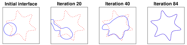
Figure 4.1: Optimization process for case 1

Case 2: We demonstrate how the proposed algorithm can handle an interface inverse/design problem whose target interface consists of multiple closed curves. For this purpose and for simplicity, we consider the case in which interface $\Gamma$ is formed by the two simple curves such that $S(x,y)=0$. We denote the sub-domain inside the upper-left dotted curve (in red color) by $\Omega^{1}$, the sub-domain inside the lower-right dotted curve (in red color) by $\Omega^{2}$, and denote sub-domain outside these two closed dotted curve by $\Omega^{3}$, see Figure 4.2. The interface problem described by (LABEL:inter_prob_0) and (LABEL:jump_cond_0) and its corresponding IFE discretization can be readily modified to suit the present interface configuration in which the parameter $\beta$ is a piecewise constant function such that its value on $\Omega_{i}$ is $\beta^{i}$, $i=1,2,3$. The data $\bar{u}$ for this problem is given on the whole domain $\Omega$ on which a $80\times 80$ mesh is utilized. Each numerical curve component is a parametric cubic spline with 15 control points and 30 control points in total. As demonstrated in Figure 4.2, the approximate curves by the proposed IFE method evolve from the initial approximate curve components $S_{0}^{1}$ and $S_{0}^{2}$ to the target curve components after 110 iterations. We notice that the numerical curve component started from $S_{0}^{1}$ converges to the exact curve component much faster than that started from $S_{0}^{2}$. After 10 iterations, the first numerical curve component is already quite close to the target curve, while the evolution of the second numerical curve component is obviously less. We believe the objective function is more sensitive to the design variables for the first numerical curve component than the second because the jump $\beta^{3}/\beta^{1}$ is much larger than $\beta^{3}/\beta^{2}$ in this example, and the gradient in the proposed IFE method is capable to capture this kind of subtle dependence of the objective function on the design variables.

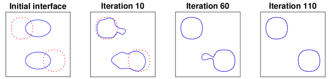
Figure 4.2: Optimization process for case 2

Case 3: The data function $\bar{u}$ is given in proper sub-domain $\Omega_{0}=[-0.5,1]\times[0,1]$ in the upper-right of $\Omega$ illustrated in Figure 4.3, with $\Omega_{0}^{s}=\Omega_{0}\cap\Omega^{s},s=\pm$. We also implement the algorithm on a $80\times 80$ mesh for this example. The numerical curve is a parametric cubic spline with 20 control points. As presented in Figure 4.3, the numerical curve converges in about 80 iterations. We observe that the converged numerical curve is a much better approximation to the target interface curve $\Gamma$ inside $\Omega_{0}$ than outside, and we believe this is a reasonable consequence of the available data function $\bar{u}$ given only on $\Omega_{0}$, and we think this example suggests again that the gradient in the proposed IFE method can capture the nature of the interface inverse problem in accordance with the available data.

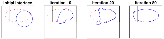
Figure 4.3: Optimization process for case 3

4.2 The Dirichlet-Neumann Problem with a Single Measurement

In this group of numerical examples, we apply the propose IFE method to the popular but challenging inverse Dirichlet-Neumann problem in which we try to recover the interface $\Gamma$ from one Neumann data $g_{N}$ provided on the boundary for an interface forward problem of the elliptic equation described by (LABEL:inter_prob_0)-(1.3) with a pure Dirichlet boundary condition. This type of inverse problems have a wide range of applications in electronic impendence tomography (EIT) [8, 37, 53] where one wishes to detect a material interface by injecting the voltage potential $g_{D}$ on $\partial\Omega$ and measuring the current density $g_{N}$ on (or a portion of) $\partial\Omega$. When the charge source $f=0$, it is referred as the Calderón’s inverse conductivity problem [12] which is well-known ill-conditioned since only the data on the boundary $\partial\Omega$ is available for the reconstruction of $\Gamma$.

We formulate this inverse problem as a shape optimization problem with a Kohn-Vogelius type functional [45, 60]:

$$\mathcal{J}(u^{1}(\Gamma),u^{2}(\Gamma),\Gamma)=\int_{\Omega}|u^{1}-u^{2}|^{2}dX,$$ (4.15)

where as in [8], $u^{1}$ and $u^{2}$ are the solutions of the following interface forward problems:

$$\begin{aligned} &\begin{cases}-\nabla\cdot(\beta\nabla u^{1})=f,\\ [u^{1}]|_{\Gamma}=0,\\ [\beta\nabla u\cdot\mathbf{n}]|_{\Gamma}=0,\\ u^{1}=g^{1}_{D}=g_{D},~{}~{}~{}\textrm{on}\;\partial\Omega,\\ \end{cases}\\ \end{aligned} \begin{aligned} &\begin{cases}-\nabla\cdot(\beta\nabla u^{2})=f,\\ [u^{2}]|_{\Gamma}=0,\\ [\beta\nabla u^{2}\cdot\mathbf{n}]|_{\Gamma}=0,\\ u^{2}=g^{2}_{D}=g_{D},~{}~{}~{}\textrm{on}\;\partial\Omega_{D},~{}~{}\frac{\partial u^{2}}{\partial\mathbf{n}}=g_{N}^{2},~{}~{}~{}\textrm{on}\;\partial\Omega_{N},\end{cases}\end{aligned}$$

and $\int_{\Omega}u^{2}dx=u_{0}$ needs to be imposed when $\partial\Omega_{N}=\partial\Omega$. Again, we employ the IFE method proposed in (LABEL:discrt_obj_2) to solve this interface inverse problem by seeking the design variable ${\boldsymbol{\alpha}}^{*}$ that minimizes the following objective function

$$\begin{split}&\mathcal{J}_{h}({\bf u}_{h}^{1}({\boldsymbol{\alpha}}),{\bf u}_{h}^{2}({\boldsymbol{\alpha}}),{\boldsymbol{\alpha}})=\int_{\Omega_{0}}J_{h}({\bf u}_{h}^{1}({\boldsymbol{\alpha}}),{\bf u}_{h}^{2}({\boldsymbol{\alpha}}),X({\boldsymbol{\alpha}}),{\boldsymbol{\alpha}})dX,\\ \text{subject to}~{}~{}~{}~{}~{}~{}&\mathbf{A}^{k}(X({\boldsymbol{\alpha}}),{\boldsymbol{\alpha}}){\bf u}_{h}^{k}(\alpha)-{\bf F}^{k}(X({\boldsymbol{\alpha}}),{\boldsymbol{\alpha}})=\mathbf{0},~{}~{}k=1,2,\end{split}$$ (4.16)

where $J_{h}({\bf u}_{h}^{1}({\boldsymbol{\alpha}}),{\bf u}_{h}^{2}({\boldsymbol{\alpha}}),X({\boldsymbol{\alpha}}),{\boldsymbol{\alpha}})=\big{(}{\tilde{J}}_{h}({\bf u}_{h}^{1}({\boldsymbol{\alpha}}),{\bf u}_{h}^{2}({\boldsymbol{\alpha}}),X({\boldsymbol{\alpha}}),{\boldsymbol{\alpha}})\big{)}^{2}$ with

$${\tilde{J}}_{h}({\bf u}_{h}^{1}({\boldsymbol{\alpha}}),{\bf u}_{h}^{2}({\boldsymbol{\alpha}}),X({\boldsymbol{\alpha}}),{\boldsymbol{\alpha}})=\sum^{|\mathring{\mathcal{N}}_{h}|}_{i=1}u^{1}_{i}\phi_{i}(X)+\sum^{|\mathcal{N}_{h}^{m}|}_{i=|\mathring{\mathcal{N}}_{h}|+1}g_{D}(X_{i})\phi_{i}(X)-\sum^{|\mathcal{N}^{m}_{h}|}_{i=1}u^{2}_{i}\phi_{i}(X).$$ (4.17)

By a similar argument to (LABEL:optimal_shape_fun_eq_3), we can show this discretized shape functional still has the optimal second order accuracy for approximating the original one on an fixed mesh. Also, similar to (4.4)-(4.14) in the output-least-squares problem discussed in Section 4.1, formulas for $\nabla J_{h}$, $\frac{\partial J_{h}}{\partial\alpha_{j}},j\in\mathcal{D}$ as well as $\frac{\partial\mathcal{J}_{h}}{\partial\mathbf{u}^{1}_{h}}$ and $\frac{\partial\mathcal{J}_{h}}{\partial\mathbf{u}^{2}_{h}}$ can be readily derived and implemented in the IFE framework, and these preparations can then be used in the proposed IFE Shape Optimization Algorithm presented in Section 3.5.

For the Dirichlet-Neumann inverse problem, we report $3$ experiments that are configured with the target curve $S(x,y)=0$ and exact solution to the interface forward problem $u(x,y)$ given in Table 4.2. We note that $u(x,y)$ given in this table is used only to generate the Dirichlet and Neumann boundary data for the related inverse problem. As before, the BFGS algorithm [59] is employed to carry out the shape optimization described by (LABEL:J_2_h) according to the proposed IFE Shape Optimization Algorithm, for which, $S_{0}(x,y)=0$ given in Table 4.2 is the initial curve that is plotted as a solid curve (in blue color) in the related figures as all other presented approximate curves in the BFGS iterations. In addition, we refine the mesh once the optimization has stalled at a certain numerical curve, i.e., the reconstructed interface curve is not moving, to obtain better reconstruction.

Cases	$\beta$	Interface $S$ and initial guess	Exact $u$
Case 1	$\left.\begin{array}[]{c}\beta^{-}=1\\ \beta^{+}=10\end{array}\right.$	$\left.\begin{array}[]{c}S=r-1,~{}\textrm{where}~{}r=(100(x-0.4)^{2}+36(y+0.3)^{2})/\pi^{2}\\ S_{0}=(x-0.1)^{2}+y^{2}-(\pi/4)^{2}\end{array}\right.$	$\begin{aligned} &u=\frac{3600}{\pi^{4}\beta^{s}}(r^{\frac{5}{2}}-1)\\ &+\frac{3600}{\pi^{4}\beta^{-}}~{}\textrm{in}~{}\Omega^{s}~{}s=\pm\end{aligned}$
Case 2	$\left.\begin{array}[]{c}\beta^{-}=1\\ \beta^{+}=2\end{array}\right.$	$\left.\begin{array}[]{c}S=(2((x+0.5)^{2}+y^{2})-x-0.2)^{2}-((x+0.5)^{2}+y^{2})+0.3\\ S_{0}=64(x-0.5)^{2}+16y^{2}-\pi^{2}\end{array}\right.$	$\begin{aligned} u=&S/\beta^{s}~{}\textrm{in}~{}\Omega^{s},\\ &s=\pm\end{aligned}$
Case 3	$\left.\begin{array}[]{c}\beta^{-}=1,\\ \beta^{+}=2\end{array}\right.$	$\left.\begin{array}[]{c}S=\sin{(\pi x)}+\frac{\pi}{1.5}y+0.1\\ S_{0}=y+0.15/\pi\end{array}\right.$	$\begin{aligned} u=&S/\beta^{s}~{}\textrm{in}~{}\Omega^{s},\\ &s=\pm\end{aligned}$

Table 4.2: Configuration for the Dirichlet-Neumann Problem

Case 1: The Neumann data is given on the whole $\partial\Omega$. The numerical curve is a parametric cubic spline with 20 control points. Some representative approximate curves generated in the optimization are plotted as solid curves (with blue color) in Figure 4.4 in which the dotted curve (in red color) is the target curve to be recovered. These numerical results demonstrate that the propose IFE method can handle a large shape change, as illustrated in Figure 4.4 from the initial interface to the one generated by the third iteration. We note that such a large shape change often causes mesh distortion when body fitting mesh is used, but the proposed IFE method totally avoid this issue by the using a fixed interface independent mesh. The first 30 iterations are generated on a $80\times 80$ mesh. The final result is generated on a $320\times 320$ mesh. Clearly, with a finer mesh we can obtain more accurate reconstruction. The numerical curve quickly converges to the target curve after about $80$ iterations, and this demonstrates again the benefit of the fact that the objective function in the proposed algorithm is a good approximation of the continuous objective functional defined by (4.15) and the gradient of the objective function in the proposed algorithm provides a good sensitivity with respect to design variables in the numerical curve.

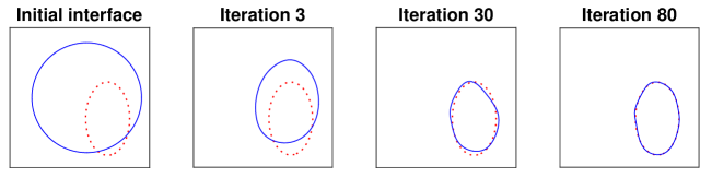
Figure 4.4: Reconstruction process for case 1

Case 2: We now consider a more difficult Dirichlet-Neumann interface inverse problem whose exact solution interface curve $\Gamma$ is non-conical and non-convex with a kidney-like shape plotted as dotted curve (in red color) in Figure 4.5, and, to the best of our knowledge, there is no general theory to guaranty the uniqueness of the solution to this inverse problem with only one single pair of Dirichelt and Neumann data. The Neumann data is given on the whole $\partial\Omega$. The numerical curve is a parametric cubic spline with 20 control points. In this case, we present 4 plots in Figure 4.5: the first one is the initial guess, and the 2nd, 3rd and 4th plots are obtained on a $80\times 80$, $160\times 160$ and $320\times 320$ mesh, respectively. Even on a relatively coarse $80\times 80$ mesh, our algorithm can capture the basic feature of the target curve to be recovered. Again, we can observe that finer mesh can push the numerical curve to the exact target curve, but this process takes far more iterations than Case 1. We believe this is caused by the challenging nature of this interface inverse problem whose exact solution is non-convex; nevertheless, the proposed IFE method still produces an approximate solution quite satisfactory to a certain extend.

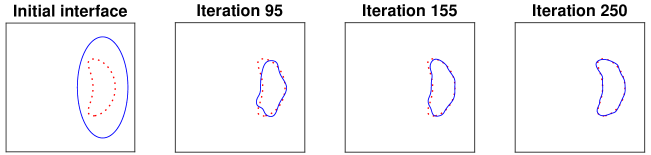
Figure 4.5: Reconstruction process for case 2

Case 3: In this case, the Neumann data is provided only on a proper subset of the boundary $\partial\Omega$. Specifically, the true interface $\Gamma$ is the level set $S(x,y)=0$ plotted as the dotted curve (in red color) in Figure 4.6 that separates $\Omega$ into two sub-domains $\Omega^{-}$ and $\Omega^{+}$ below and above $\Gamma$, and the Neumann data function $g_{N}$ is given only on the lower and upper edge of the square domain $\Omega$. The numerical interface is a 1-D cubic spline $y=y(t)$, $t\in[-1,1]$ with 10 control points whose end points match the exact interface. The first plot in Figure 4.6 shows the initial guess and the 2nd, 3rd and 4th plots are obtained on a $80\times 80$, $160\times 160$ and $320\times 320$ mesh, respectively. Again, the algorithm can produce a quite good reconstruction even on a coarse mesh ($80\times 80$) to a certain extend. The last plot in Figure 4.6 shows that the numerical curve after $140$ iterations matches the exact curve well, and this demonstrates that the proposed IFE method can treat a Dirichlet-Naumann interface inverse problem that has a limited Neumann data measured on part of the boundary of $\Omega$. We also test the case in which the Neumann data is on the left and right boundary of $\Omega$ instead of the lower and upper edges, but the result is not as satisfactory as the one presented here.

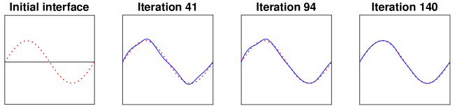
Figure 4.6: Reconstruction process for case 3

4.3 The Heat Dissipation Problem

We now consider an application of the proposed IFE method to an optimal design problem for a heat system in which the goal is to minimize the overall heat dissipation by optimally distributing two materials in a domain [24, 26, 76]. This thermal design problem has wide applications such as cooling fins [5, 66] and high-conductivity channel of electronic components [7].

In the steady heat conduction situation, this design problem is to find an optimal curve $\Gamma^{*}$ separating two chosen materials that can minimize the following objective functional [24]:

$$\mathcal{J}(u^{1}(\Gamma),\Gamma)=\int_{\Omega}\nabla u^{1}\cdot(\beta\nabla u^{1})dx\text{~{}~{}~{}subject to~{}~{}~{}}|\Omega^{1}|\leqslant\theta|\Omega|,$$ (4.18)

where $u^{1}$ is the solution to the interface problem described by (LABEL:inter_prob_0)-(LABEL:jump_cond_0) with $K=1$ with a Dirichlet boundary condition, $\Omega^{1}$ is the sub-domain filled with the high conductivity material, and $\theta\in(0,1)$ is prescribed design parameter. By the proposed IFE method (LABEL:discrt_obj_2), we seek a design variable ${\boldsymbol{\alpha}}^{*}$ that minimizes the following objective function

$$\begin{split}&\mathcal{J}_{h}({\bf u}_{h}^{1}({\boldsymbol{\alpha}}),{\boldsymbol{\alpha}})=\int_{\Omega_{0}}J_{h}({\bf u}_{h}^{1}({\boldsymbol{\alpha}}),X({\boldsymbol{\alpha}}),{\boldsymbol{\alpha}})dX,\\ \text{subject to}~{}~{}~{}~{}~{}~{}&\mathbf{A}^{1}(X({\boldsymbol{\alpha}}),{\boldsymbol{\alpha}}){\bf u}_{h}^{1}(\alpha)-{\bf F}^{1}(X({\boldsymbol{\alpha}}),{\boldsymbol{\alpha}})=\mathbf{0},\text{~{}~{}and~{}~{}}|\Omega^{1}|\leqslant\theta|\Omega|,\end{split}$$ (4.19)

where

$$J_{h}({\bf u}_{h}^{1}({\boldsymbol{\alpha}}),X({\boldsymbol{\alpha}}),{\boldsymbol{\alpha}})=\beta\left|\sum^{|\mathring{\mathcal{N}}_{h}|}_{i=1}u_{i}^{1}\nabla\phi_{i}(X)+\sum^{|\mathcal{N}_{h}|}_{i=|\mathring{\mathcal{N}}_{h}|+1}g_{D}(X_{i})\nabla\phi_{i}(X)\right|^{2}.$$ (4.20)

Since the objective functional involves gradients, following the idea in derivation (LABEL:optimal_shape_fun_eq_3), we can show that the discretized functional can approximate the true shape functional with an optimal first order accuracy independent of the interface shape and location. Also, similar to (4.4)-(4.14) again, formulas can be derived for $\mathcal{J}_{h}({\bf u}_{h}^{1}({\boldsymbol{\alpha}}),{\boldsymbol{\alpha}})$, $\frac{\partial J_{h}}{\partial\alpha_{j}},j\in\mathcal{D}$ and $\frac{\partial\mathcal{J}_{h}}{\partial\mathbf{u}_{h}^{1}}$ within the IFE framework. In particular, we have $\nabla J_{h}={\bf 0}$. These preparations can then be employed in the proposed IFE Shape Optimization Algorithm together with the SQP (sequential quadratic programming) method [59] to carry out the constrained optimization numerically.

We test the proposed IFE method on a specific design problem configured in the domain $\Omega$ that contains a design independent heat source $f=-1$ on a center square $[-0.1,0.1]\times[-0.1,0.1]$, the boundary temperature is fixed to be $u=0$ and $\theta=0.5$, see the illustration in Figure 4.7. The two materials separated by the curve $\Gamma$ are such that $\beta^{-}=1$ and $\beta^{+}=10^{-3}$. We start the SQP iteration from a circle $x^{2}+y^{2}=0.82^{2}$ plotted as a solid curve (in blue color) in Figure 7(b)(a), and the numerical curve in the optimization is a parametric cubic spline with 20 control points. We use the $160\times 160$ mesh in this example. After 28 iterations, the proposed algorithm generates a design shown in Figure 4.7(b) whose patten is very similar to the one reported in [24].

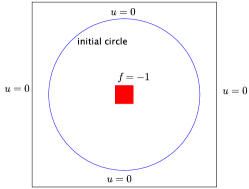
(a) The heating conditions and initial guess

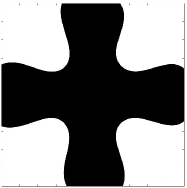
(b) The optimal design

Figure 4.7: The heat dissipation problem

References

- [1] Slimane Adjerid, Nabil Chaabane, and Tao Lin. An immersed discontinuous finite element method for stokes interface problems. Comput. Methods Appl. Mech. Engrg., 293:170–190, 2015.
- [2] G. Alessandrini, V. Isakov, and J. Powell. Local uniqueness in the inverse conductivity problem with one measurement. Transactions of the American Mathematical Society, 347(8):3031–3041, 1995.
- [3] G. Allaire, C. Dapogny, and P. Frey. Shape optimization with a level set based mesh evolution method. Comput. Methods Appl. Mech. Engrg., 282:22–53, 2014.
- [4] Grégoire Allaire, François Jouve, and Anca-Maria Toader. Structural optimization using sensitivity analysis and a level-set method. J. Comput. Phys., 194(1):363–393, 2004.
- [5] A. V. Attetkov, I. K. Volkov, and E. S. Tverskaya. The optimum thickness of a cooled coated wall exposed to local pulse‐periodic heating. J. Eng. Phys. Thermophys., 74(6):1467–1474, 2001.
- [6] Ivo Babuška and John E. Osborn. Can a finite element method perform arbitrarily badly? Math. Comp., 69(230):443–462, 2000.
- [7] Adrian Bejan. Constructal-theory network of conducting paths for cooling a heat generating volume. Int. J. Heat Mass Transfer, 40(4):799,813–811,816, 1997.
- [8] Z. Belhachmi and H. Meftahi. Shape sensitivity analysis for an interface problem via minimax differentiability. Appl. Math. Comput., 219(12):6828, 2013.
- [9] Martin P. Bendsøe. Optimization of structural topology, shape, and material. Springer-Verlag, Berlin, 1995.
- [10] Susanne C. Brenner and L. Ridgway Scott. The mathematical theory of finite element methods, volume 15 of Texts Appl. Math. Springer, New York, third edition, 2008.
- [11] Martin Burger and Stanley J. Osher. A survey on level set methods for inverse problems and optimal design. European J. Appl. Math., 16(2):263–301, 2005.
- [12] Alberto P. Calderón. On an inverse boundary value problem. Comput. Appl. Math, 25(2-3), 2006.
- [13] Alejandro Cantarero and Tom Goldstein. A fast method for interface and parameter estimation in linear elliptic pdes with piecewise constant coefficients. 2013.
- [14] G. Carpentieri, B. Koren, and M. J. L. van Tooren. Adjoint-based aerodynamic shape optimization on unstructured meshes. J. Comput. Phys., 224(1):267–287, 2007.
- [15] Tony F. Chan and Xue-Cheng Tai. Identification of discontinuous coefficients in elliptic problems using total variation regularization. SIAM J. Sci. Comput, 25(3):881–904, 2003.
- [16] Zhiming Chen, Zedong Wu, and Yuanming Xiao. An adaptive immersed finite element method with arbitrary lagrangian-eulerian scheme for parabolic equations in time variable domains. Int. J. Numer. Anal. Mod., pages 567–591, 2015.
- [17] Zhiming Chen and Jun Zou. Finite element methods and their convergence for elliptic and parabolic interface problems. Numer. Math., 79(2):175–202, 1998.
- [18] Zhiming Chen and Jun Zou. An augmented lagrangian method for identifying discontinuous parameters in elliptic systems. SIAM J. Control Optim., 37(3), 1999.
- [19] Kyung K. Choi and Kuang-Hua Chang. A study of design velocity field computation for shape optimal design. Finite Elem. Anal. Des., 15(4):317–341, 1994.
- [20] S. Chow and R. S. Anderssen. Determination of the transmissivity zonation using a linear functional strateg. Inverse Problems, 7:841, 1991.
- [21] J.E. Dennis and Robert B. Schnabel. Numerical Methods for Unconstrained Optimization and Nonlinear Equations, volume 16 of Classics Appl. Math. SIAM, 1996.
- [22] Peter D. Dunning, H. A. Kim, and Glen Mullineux. Investigation and improvement of sensitivity computation using the area-fraction weighted fixed grid fem and structural optimization. Finite Elem. Anal. Des., 47(8):933–941, 2011.
- [23] Richard E. Ewing, Society for Industrial, and Applied Mathematics. The Mathematics of reservoir simulation, volume 1. SIAM, Philadelphia, 1983.
- [24] T. Gao, W. H. Zhang, J. H. Zhu, Y. J. Xu, and D. H. Bassir. Topology optimization of heat conduction problem involving design-dependent heat load effect. Finite Elem. Anal. Des., 44(14):805–813, 2008.
- [25] Walter Gautschi. Numerical analysis. Springer / Birkhäuser, New York, 2nd edition, 2012.
- [26] A. Gersborg-Hansen, M. P. Bendsøe, and O. Sigmund. Topology optimization of heat conduction problems using the finite volume method. Struct. Multidiscip. Optim., 31(4):251–259, 2006.
- [27] Michael B. Giles and Niles A. Pierce. An introduction to the adjoint approach to design. Flow Turbul. Combust., 65(3):393–415, 2000.
- [28] Mark S. Gockenbach and Akhtar A. Khan. An abstract framework for elliptic inverse problems: Part 2. an augmented lagrangian approach. Math. Mech. Solids, 14(6):517–539, 2009;2008;.
- [29] Ruchi Guo and Tao Lin. A group of immersed finite element spaces for elliptic interface problems. arXiv:1612.01862, 2016.
- [30] Ruchi Guo, Tao Lin, and Xu Zhang. Nonconforming immersed finite element spaces for elliptic interface problems. arXiv:1612.01862, 2016.
- [31] Helmut Harbrecht and Johannes Tausch. On the numerical solution of a shape optimization problem for the heat equation. SIAM J. Sci. Comput., 35(1):A.104–A121, 2013.
- [32] J. Haslinger and R. A. E. Mäkinen. Introduction to shape optimization: theory, approximation, and computation. SIAM, Society for Industrial and Applied Mathematics, Philadelphia, 2003.
- [33] Xiaoming He, Tao Lin, and Yanping Lin. Approximation capability of a bilinear immersed finite element space. Numer. Methods Partial Differential Equations, 24(5):1265–1300, 2008.
- [34] Xiaoming He, Tao Lin, and Yanping Lin. Immersed finite element methods for elliptic interface problems with non-homogeneous jump conditions. Int. J. Numer. Anal. Model., 8(2):284–301, 2011.
- [35] Jan Hegemann, Alejandro Cantarero, Casey L. Richardson, and Joseph M. Teran. An explicit update scheme for inverse parameter and interface estimation of piecewise constant coefficients in linear elliptic pdes. SIAM J. Sci. Comput., 35(2), 2013.
- [36] Cosmina Hogea, Christos Davatzikos, and George Biros. An image-driven parameter estimation problem for a reaction–diffusion glioma growth model with mass effects. J. Math. Biol., 56(6):793–825, 2008.
- [37] David Holder and Institute of Physics (Great Britain). Electrical impedance tomography: methods, history, and applications. Institute of Physics Pub, 2005.
- [38] X. Huang and Y. M. Xie. Evolutionary topology optimization of continuum structures: methods and applications. Wiley, Hoboken, NJ;Chichester, West Sussex, U.K;, 2010.
- [39] Kazufumi Ito and Karl Kunisch. The augmented lagrangian method for parameter estimation in elliptic systems. SIAM J. Control Optim., 28(1):113–136, 1990.
- [40] Kazufumi Ito, Karl Kunisch, and Zhilin Li. Level-set function approach to an inverse interface problem. Inverse Problems, 17:1225, 2001.
- [41] Gang-Won Jang and Yoon Y. Kim. Sensitivity analysis for fixed-grid shape optimization by using oblique boundary curve approximation. Int J Solids Struct., 42(11):3591–3609, 2005.
- [42] Lin Ji, Joyce R. McLaughlin, Daniel Renzi, and Jeong-Rock Yoon. Interior elastodynamics inverse problems: shear wave speed reconstruction in transient elastography. Inverse Problems, 19(6):S1–S29, 2003.
- [43] H. Kim, O. M. Querin, G. P. Steven, and Y. M. Xie. Improving efficiency of evolutionary structural optimization by implementing fixed grid mesh. Struct. Multidiscip. Optim., 24(6):441–448, 2002.
- [44] Nam H. Kim and Youngmin Chang. Eulerian shape design sensitivity analysis and optimization with a fixed grid. Comput. Methods Appl. Mech. Engrg., 194(30):3291–3314, 2005.
- [45] Robert V. Kohn and Michael Vogelius. Relaxation of a variational method for impedance computed tomography. Commun. Pure Appl. Anal., 40(6):745–777, 1987.
- [46] Hae S. Lee, Cheon J. Park, and Hyun W. Park. Identification of geometric shapes and material properties of inclusions in two-dimensional finite bodies by boundary parameterization. Comput. Methods Appl. Mech. Engrg., 181(1):1–20, 2000.
- [47] Qing Li, Grant P. Steven, Y. M. Xie, and Osvaldo M. Querin. Evolutionary topology optimization for temperature reduction of heat conducting fields. Int. J. Heat Mass Transfer, 47(23):5071–5083, 2004.
- [48] Zhilin Li, Tao Lin, Yanping Lin, and Robert C. Rogers. An immersed finite element space and its approximation capability. Numer. Methods Partial Differential Equations, 20(3):338–367, 2004.
- [49] Zhilin Li, Tao Lin, and Xiaohui Wu. New Cartesian grid methods for interface problems using the finite element formulation. Numer. Math., 96(1):61–98, 2003.
- [50] Tao Lin, Yanping Lin, Robert Rogers, and M. Lynne Ryan. A rectangular immersed finite element space for interface problems. In Scientific computing and applications (Kananaskis, AB, 2000), volume 7 of Adv. Comput. Theory Pract., pages 107–114. Nova Sci. Publ., Huntington, NY, 2001.
- [51] Tao Lin, Yanping Lin, and Xu Zhang. Partially penalized immersed finite element methods for elliptic interface problems. SIAM J. Numer. Anal., 53(2):1121–1144, 2015.
- [52] Tao Lin and Xu Zhang. Linear and bilinear immersed finite elements for planar elasticity interface problems. J. Comput. Appl. Math., 236(18):4681–4699, 2012.
- [53] W. R. B. Lionheart. Boundary shape and electrical impedance tomography. Inverse Problems, 14:139, 1998.
- [54] Zhen Luo, Michael Y. Wang, Shengyin Wang, and Peng Wei. A level set-based parameterization method for structural shape and topology optimization. International Journal for Numerical Methods in Engineering, 76(1):1–26, 2008.
- [55] Joyce R. McLaughlin, Ning Zhang, and Armando Manduca. Calculating tissue shear modulus and pressure by 2d log-elastographic methods. Inverse Problems, 26, 2010.
- [56] Bijan Mohammadi and Olivier Pironneau. Shape optimization in fluid mechanics. Annu. Rev. Fluid Mech., 36(1):255–279, 2004.
- [57] Ahmad R. Najafi, Masoud Safdari, Daniel A. Tortorelli, and Philippe H. Geubelle. A gradient-based shape optimization scheme using an interface-enriched generalized fem. Comput. Methods Appl. Mech. Engrg., 296:1–17, 2015.
- [58] S. S. Nanthakumar, T. Lahmer, and T. Rabczuk. Detection of flaws in piezoelectric structures using extended fem. International Journal for Numerical Methods in Engineering, 96(6):373–389, 2013.
- [59] J. Nocedal and S. Wright. Numerical optimization. Springer Series in Operations Research. Springer, second edition, 2006.
- [60] Antonio André Novotny, Alfredo Canelas, and Antoine Laurain. A non-iterative method for the inverse potential problem based on the topological derivative. In Technical Report for Mini-Workshop: Geometries, Shapes and Topologies in PDE-based Applications, 57/2012, edited by Michael Hintermüller and Günter Leugering and Jan Sokołowski, pages 3383–3387, Mathematisches Forschungsinstitut Oberwolfach, Oberwolfach, Germany, 2012.
- [61] Antonio André Novotny and Jan Sokołowski. Topological derivatives in shape optimization. Springer, Heidelberg, 2013.
- [62] X. Peng, K. Niakhai, and B. Protas. A method for geometry optimization in a simple model of two-dimensional heat transfer. SIAM J. Sci. Comput., 35(5):B.1105–B1131, 2013.
- [63] Mauro Perego, Alessandro Veneziani, and Christian Vergara. A variational approach for estimating the compliance of the cardiovascular tissue: An inverse fluid-structure interaction problem. SIAM J. Sci. Comput., 33(3):1181–1211, 2011.
- [64] Daniel Rabinovich, Dan Givoli, and Shmuel Vigdergauz. Xfem-based crack detection scheme using a genetic algorithm. International Journal for Numerical Methods in Engineering, 71(9):1051–1080, 2007.
- [65] J. J. Ródenas, F. J. Fuenmayor, and J. E. Tarancón. A numerical methodology to assess the quality of the design velocity field computation methods in shape sensitivity analysis. Internat. J. Numer. Methods Engrg., 59(13):1725–1747, 2004.
- [66] M. Sasikumar and C. Balaji. Optimization of convective fin systems: a holistic approach. Heat Mass Transf., 39(1):57–68, 2002.
- [67] David H. Sattinger, C. A. Tracy, and S. Venakides. Inverse scattering and applications, volume 122. American Mathematical Society, Providence, R.I, 1991.
- [68] D. S. Schnur and Nicholas Zabaras. An inverse method for determining elastic material properties and a material interface. Internat. J. Numer. Methods Engrg., 33(10):2039–2057, 1992.
- [69] Soheil Soghrati, Alejandro M. Aragón, C. Armando Duarte, and Philippe H. Geubelle. An interface‐enriched generalized fem for problems with discontinuous gradient fields. Internat. J. Numer. Methods Engrg., 89(8):991–1008, 2012.
- [70] Katsuyuki Suzuki and Noboru Kikuchi. A homogenization method for shape and topology optimization. Comput. Methods Appl. Mech. Engrg., 93(3):291–31, 1991.
- [71] Haim Waisman, Eleni Chatzi, and Andrew W. Smyth. Detection and quantification of flaws in structures by the extended finite element method and genetic algorithms. International Journal for Numerical Methods in Engineering, 2009.
- [72] Peng Wei, Michael Y. Wang, and Xianghua Xing. A study on x-fem in continuum structural optimization using a level set model. Comput. Aided Des., 42(8):708–719, 2010.
- [73] William W. Yeh. Review of parameter identification procedures in groundwater hydrology: The inverse problem. Water Resources Research, 22(2):95–108, 1986.
- [74] J. Zhang, W. H. Zhang, J. H. Zhu, and L. Xia. Integrated layout design of multi-component systems using xfem and analytical sensitivity analysis. Comput. Methods Appl. Mech. Engrg., 245-246:75–89, 2012.
- [75] Xu Zhang. Nonconforming Immersed Finite Element Methods for Interface Problems. 2013. Thesis (Ph.D.)–Virginia Polytechnic Institute and State University.
- [76] Yongcun Zhang, Shutian Liu, and Heting Qiao. Design of the heat conduction structure based on the topology optimization. Dev. Heat Transf., 2011.