Constraining the coherence scale of the interstellar magnetic field using TeV gamma-ray observations of supernova remnants

Abstract

Galactic cosmic rays (CRs) are believed to be accelerated at supernova remnant (SNR) shocks. In the hadronic scenario the TeV gamma-ray emission from SNRs originates from decaying pions that are produced in collisions of the interstellar gas and CRs. Using CR-magnetohydrodynamic simulations, we show that magnetic obliquity-dependent shock acceleration is able to reproduce the observed TeV gamma-ray morphology of SNRs such as Vela Jr. and SN1006 solely by varying the magnetic morphology. This implies that gamma-ray bright regions result from quasi-parallel shocks (i.e., when the shock propagates at a narrow angle to the upstream magnetic field), which are known to efficiently accelerate CR protons, and that gamma-ray dark regions point to quasi-perpendicular shock configurations. Comparison of the simulated gamma-ray morphology to observations allows us to constrain the magnetic coherence scale $\lambda_{B}$ around Vela Jr. and SN1006 to $\lambda_{B}\simeq 13_{-4.3}^{+13}$ pc and $\lambda_{B}>200_{-10}^{+80}$ pc, respectively, where the ambient magnetic field of SN1006 is consistent with being largely homogeneous. We find consistent pure hadronic and mixed hadronic-leptonic models that both reproduce the multi-frequency spectra from the radio to TeV gamma rays and match the observed gamma-ray morphology. Finally, to capture the propagation of a SNR shock in a clumpy interstellar medium, we study the interaction of a shock with a dense cloud with numerical simulations and analytics. We construct an analytical gamma-ray model for a core collapse SNR propagating through a structured interstellar medium, and show that the gamma-ray luminosity is only biased by 30% for realistic parameters.

1 Introduction

SNR shocks energize Galactic CRs via diffusive shock acceleration. This converts about $5-10\%$ of the kinetic energy into a non-thermal, power-law momentum distribution of CRs (Bell, 1978; Blandford & Ostriker, 1978). The most direct observational evidence for this is the GeV and TeV gamma-ray emission from SNRs. There are two competing models: in the leptonic model, CR electrons Compton upscatter (interstellar) radiation fields whereas in the hadronic model inelastic collisions between the interstellar medium (ISM) and CRs produce neutral pions that decay into gamma rays (Hinton & Hofmann, 2009; Zirakashvili & Aharonian, 2010). The latter process produces a kinematic spectral feature below GeV energies, as recently observed by the Fermi gamma-ray telescope (Ackermann et al., 2013). However, the steep high-energy spectral slope raises questions whether this represents an unambiguous proof of CR hadron acceleration at this SNR (Cardillo et al., 2016).

The hadronic model requires efficient CR hadrons acceleration, which must be accompanied by substantial magnetic field amplification via the hybrid non-resonant instability (Bell, 2004). This finding received strong observational support with the detection of thin X-ray synchrotron filaments at several SNR shocks. Those filaments exhibit fast (year-scale) variability and likely result from cooling of freshly accelerated electrons in magnetic fields of $\approx 1\,$mG (Uchiyama et al., 2007). Spatial correlations between gamma-ray brightness and gas column density are another consequence of the hadronic model and are expected for core-collapse supernovae, which explode inside molecular clouds due to the fast evolution of their massive progenitor stars. Combining synchrotron and inverse Compton emission in the leptonic model yields volume-filling magnetic field strengths of $\approx 10\,\mu$G (Gabici & Aharonian, 2016), which are compatible with mG-field strengths inferred from X-ray synchrotron filaments only when assuming a clumpy medium. It has also been argued that a rising gamma-ray energy spectrum with increasing photon energy provides evidence for leptonic models. However, such a spectrum can also be obtained in the hadronic model when considering a clumpy ISM because of proton propagation effects that substantially harden the proton spectrum inside dense clumps in comparison to the acceleration spectrum in the diffuse ISM (Gabici & Aharonian, 2014; Celli et al., 2019). The absence of thermal X–rays from the remnant provides additional support for this scenario because the shock will considerably slow down while penetrating into dense clumps and thus cannot heat them up to X-ray emitting temperatures (Inoue et al., 2012).

Alternatively, leptonic scenarios have been proposed to explain the gamma-ray emission from young SNRs in an ISM model with homogeneous density (e.g., Pohl, 1996) in order to overcome the lack of thermal X-ray emission. This results in a low upper limit on the ISM density. Leptonic models evoke inverse Compton (IC) scattering of CR electrons with a photon field that is provided by the ubiquitous cosmic microwave background in combination with (dust-processed) stellar light. For example, Xing et al. (2016) uses leptonic models to explain the emission from the South-Western limb of SN1006 while this explanation is extended to the entire remnant (Petruk et al., 2011; Araya & Frutos, 2012). The leptonic scenario naturally explains the correlation between X-ray synchrotron and IC gamma-ray emitting regions such as in Vela Jr. (Aharonian et al., 2007) and matches the observed broadband spectrum. On the other hand, this model implies low magnetic field strengths, which are in contradiction to the narrow filamentary structures detected in X-rays. Hence, we need to understand the detailed spatial structure of SNRs across different wave lengths to unambiguously identify emission and particle acceleration processes.

The high angular resolution ($<0.1^{\circ}$) of imaging air Čerenkov telescopes H.E.S.S., VERITAS, and MAGIC enables detailed morphological gamma-ray studies of SNRs and to separate or exclude contributions by compact sources such as pulsars. In particular, TeV gamma-ray observations have delivered a rich morphology of shell-type SNRs, ranging from the bi-lobed emission of SN1006 (H.E.S.S. Collaboration, 2010) to the filamentous, patchy appearances of Vela Jr. (H.E.S.S. Collaboration, 2018b) and RX-J1713 (H.E.S.S. Collaboration, 2018a), to the young, type Ia SNR Tycho G120.1+01.4 (Archambault et al., 2017). In principle, the patchy gamma-ray morphology could result from density inhomogeneities (Berezhko & Völk, 2008; Atoyan et al., 2000) of the ambient ISM. It yet remains to be seen whether the fluctuation amplitude necessary for the observed gamma-ray patchiness does not introduce a corrugated shock surface (Ji et al., 2016) that is inconsistent with the observed spherical blast wave.

Here, we propose a different model in which the acceleration process imprints a rich gamma-ray morphology due to the global magnetic morphology (Pais et al., 2018). Hybrid particle-in-cell simulations of non-relativistic, strong shocks show that diffusive shock acceleration of hadrons efficiently operates for quasi-parallel configurations (i.e., when the shock propagates along the upstream magnetic field or moves at a narrow angle to it) and converts around 15% of the available energy to CRs (Caprioli & Spitkovski, 2014). In contrast, a shock that propagates perpendicular to the magnetic field (or at a large angle to it, i.e., a quasi-perpendicular configuration) is an inefficient accelerator without strong pre-existing turbulence at the CR gyroscale (Giacalone et al., 1992) because charged particles are bound to gyrate around the flux-frozen magnetic field. As the magnetized plasma sweeps past the shock, so are the gyrating particles, which cannot return back upstream.

We aim to explain the apparently disparate TeV morphologies of SNR 1006 and Vela Jr. within a single physical model assuming a hadronic model linking gamma-ray morphology and local orientation of the magnetic field. To this end, we run a suite of simulations modeling a point explosion that encounters a range in magnetic field morphologies, from a homogeneous field to a mixture of homogeneous and turbulent fields to fully turbulent fields with varying coherence lengths in Section 2. We rescale our simulation parameters within observational limits to reproduce the observed gamma-ray spectra and flux (Section 3). Comparing simulated to observed morphologies in Section 4 allows to constrain the magnetic coherence length that the unperturbed ISM had before it encountered the SNR blast wave. Assuming statistical homogeneity, we thus constrain the magnetic coherence scale in the immediate vicinity of the SNR. We explore how the gamma-ray signal is modified by launching the SNR into stellar wind profiles instead of a homogeneous ISM environment in Section 5 and conclude in Section 6. In Appendix A, we study the interaction of a shock with a dense cloud with numerical simuations and analytics and construct an analytical model for the gamma-ray luminosity from a core collapse SNR that interacts with a structured ISM with a large population of dense, cold clouds.

2 Simulation setup

2.1 Rationale

We aim to produce realistically looking TeV gamma-ray maps with the least amount of necessary physical complexity but including all the required processes for drawing transparent and robust conclusions from our three-dimensional MHD simulations. To this end we follow the following rationale:

• The general numerical setup consists of simulating the Sedov-Taylor phase of SNRs by injecting energy at the initial time into our simulation domain that is filled with magnetized plasma with different correlation lengths. We identify the shock during the run-time of the simulations, inject CR energy at the shock with an efficiency that is in agreement with the results of ab initio particle-in-cell plasma simulations, and advect the CR energy density with the thermal plasma.

• In order to explain the TeV gamma-ray morphology for two famous shell-type SNR, SN1006 and Vela Jr., we have to realistically model the external medium that the remnant shocks are propagating into. Because the thermonuclear supernova SN1006 (of type Ia) is located at a Galactic height of 0.4 kpc, the shock propagates into low-density medium and encounters mostly homogeneous magnetic field that was potentially stretched due to a galactic outflow or the Parker instability.

• In contrast, the Vela Jr. SNR is thought to be associated with a core-collapse supernova explosion (Wang & Chevalier, 2002), which results from the collapse of a massive star. Hence, in the post-processing, we account for the free expansion phase preceeding the Sedov-Taylor phase and rescale the final radii accordingly. The Vela Jr. SNR encounters a highly structured, multiphase ISM that is typical of star forming regions. This is modelled with a population of dense gaseous clumps embedded in a nearly homogeneous background medium, which simultaneously explains the absence of thermal X-ray emission and hard TeV gamma-ray spectra in the hadronic model (Celli et al., 2019). Finally, we additionally simulate the expansion of the SNR into two different stellar wind profiles that bracket the uncertainty in the progenitor model and study its impact on the TeV gamma-ray morphology.

2.2 Simulation setup

We perform our simulations with the second-order accurate, adaptive moving-mesh code AREPO (Springel, 2010; Pakmor et al., 2016), using standard parameters for mesh regularization. Magnetic fields are treated with ideal magnetohydrodynamics (Pakmor & Springel, 2013), using the Powell scheme for divergence control (Powell et al., 1999). CRs are modelled as a relativistic fluid with adiabatic index $4/3$ in a two-fluid approximation (Pfrommer et al., 2017).

We localize and characterize shocks during the simulation (Schaal & Springel, 2015) to inject CRs into the downstream (Pfrommer et al., 2017) with an efficiency that depends on the upstream magnetic obliquity (Pais et al., 2018). We adopt a maximum acceleration efficiency for CRs at quasi-parallel shocks of $15\%$ that approaches zero for quasi-perpendicular shocks (Caprioli & Spitkovski, 2014). We only model the dominant advective CR transport and neglect CR diffusion and streaming. This is justified since diffusively shock accelerated CRs experience efficient Bohm diffusion with a coefficient $\kappa_{\mathrm{Bohm}}$ at the shock (Stage et al., 2006), which implies a CR precursor ($L_{\mathrm{prec}}$) that is smaller than our grid cells, $L_{\mathrm{prec}}\sim\sqrt{\kappa_{\mathrm{Bohm}}t}\sim 0.1~{}\mathrm{pc}\times(pc/10\,\mathrm{TeV})^{1/2}\,(B/100\,\mu\mathrm{G})^{-1/2}\,(t/10^{3}\,\mathrm{yr})^{1/2}$. We neglect slow non-adiabatic CR cooling processes in comparison to the fast Sedov expansion.

Each simulation follows a point explosion that results from depositing $E_{\mathrm{SN}}=10^{51}~{}{\rm erg}$ in a homogeneous periodic box (Pfrommer et al., 2017). This leads to an energy-driven, spherically-symmetric strong shock expanding in a low-pressure ISM with mean molecular weight $\mu=1.4$. Our initial conditions are constructed by first generating a Voronoi mesh with randomly distributed mesh-generating points in our three-dimensional simulation box with $200^{3}$ cells that we then relax via Lloyd’s algorithm (Lloyd, 1982) to obtain a glass-like configuration.

To simulate a realistic star forming environment for Vela Jr. we inserted $7\times 10^{3}$ uniformly distributed small, dense clumps with a number density of $n_{\mathrm{c}}=10^{3}~{}{\rm c}{\rm m}^{-3}$ and a diameter of $0.1~{}{\rm pc}$ (McKee & Ostriker, 1977). More details about the clumps can be found in Appendix A.

Our turbulent magnetic fields exhibit magnetic power spectra of Kolmogorov type with different coherence lengths. The three magnetic field components are treated independently so that the resulting field has a random phase. To fulfill the constraint $\boldsymbol{\nabla}\boldsymbol{\cdot}\textbf{{B}}=0$ we project out the radial field component in Fourier space. We assume a low ISM pressure of 0.44 eV cm^-3 and scale the field strength to an average plasma beta factor of unity. To ensure pressure equilibrium in the initial conditions, we adopt temperature fluctuations of the form $nk_{\mathrm{B}}\delta{}T=-\delta\textbf{{B}}^{2}/(8\pi)$ (for details, see Pais et al. 2018).

In our physical set-up, there are two different processes driving turbulence. The process of diffusive shock acceleration excites non-linear (turbulent) Bell modes on scales below the CRs’ gyroradii (Bell, 2004). Because we adopt the obliquity-dependent CR acceleration efficiency from self-consistent plasma simulations (Caprioli & Spitkovski, 2014) in our sub-grid model, we implicitly account for the full kinetic physics.

On the contrary, the magnetic turbulence that we explicitly model in our simulations reflects the supernovae-driven ISM turbulence with varying injection scales from 4 to 200 pc. The magnetic fluctuations cascade down to levels of $\delta B/B\approx 10^{-3}$ at resonant length scales of TeV CRs so that they do not interfere with the large-scale field topology at the shock. To derive this result, we assumed Alfvénic turbulence for parallelly propagating Alfvén waves according to theory of magnetohydrodynamical turbulence Goldreich & Sridhar (1995) in a mean magnetic field of $10\,\mu$G. Hence, the small fluctuation amplitude and the enormous scale separation of injection-to-gyroscale of $\approx 10^{5}$ justifies our separate treatment of these two processes.

2.3 Observational modeling

In order to connect our simulations to gamma-ray observations, we need to take into account all observational constraints on ISM properties. For practical reasons, here we derive approximate scaling laws of the gamma-ray flux in the Sedov-Taylor regime and adopt the simplified assumption of a CR spectrum with index $\alpha_{\mathrm{p}}=2$, which yields an equal contribution to the total CR energy for each decade in CR momentum. These scaling relations enable us to find parameter combinations of the SNR and surrounding ISM, which match observed gamma-ray fluxes in the hadronic model. We will vary those parameter combinations in a detailed multi-frequency analysis in Section 3 study how they vary if the SNR shock propagates in a stellar wind profile in Section 5.

2.3.1 SN1006

SN1006 represents a good case study of a SNR with a unique gamma-ray morphology. Moreover, its exactly known age allows to tightly constrain other environmental ISM parameters. Low-resolution HI measurements of the density around SN1006 suggest a diffuse density of $n=0.3~{}{\rm c}{\rm m}^{-3}$ and an interaction of the SNR with a dense cloud of $n=0.5~{}{\rm c}{\rm m}^{-3}$ (Dubner et al., 2002). Studies based on X-ray spectroscopy estimate the density of the North-Western rim of the SNR to be $n=(0.15-0.25)~{}{\rm c}{\rm m}^{-3}$ (Long et al., 2003) which is consistent with hydrodynamic simulations of an explosion energy of $10^{51}~{}{\rm erg}$ in a homogeneous medium (Wang & Chevalier, 2001). More recent papers suggest an even lower ambient density for the North-Western rim of $n=0.085~{}{\rm c}{\rm m}^{-3}$, which is estimated based on X-ray proper motion measurements (Katsuda et al., 2009), down to a density of $n=0.05~{}{\rm c}{\rm m}^{-3}$ for the South-Eastern rim, which is based on X-ray observations in combination with a shock-plasma model (Acero et al., 2007). Such low densities, however, would require an uncomfortably high explosion energy in order to explain the gamma-ray emission of SN1006 in the hadronic model. Assuming a CR proton acceleration efficiency of $10\%$ yields $E_{\mathrm{SN}}=3\times 10^{51}~{}{\rm erg}$ (H.E.S.S. Collaboration, 2010).

Integrating the differential gamma-ray flux (equation (1) of Gabici & Aharonian, 2016) yields an estimate of the TeV gamma-ray flux, $\mathcal{F}_{\gamma}$, of a SNR in the hadronic model:

$$\mathcal{F}_{\gamma}\simeq\int_{1~{}{\rm T}{\rm eV}}^{100~{}{\rm T}{\rm eV}}F_{\gamma}\mathrm{d}E_{\gamma}=\int_{1~{}{\rm T}{\rm eV}}^{100~{}{\rm T}{\rm eV}}\dfrac{4W_{\mathrm{p}}~{}E_{\gamma}^{-2}\mathrm{d}E_{\gamma}}{\ln(E_{\mathrm{max}}/E_{\mathrm{min}})\tau_{\pi^{0}}4\pi D^{2}}$$ (1)

where $\tau_{\pi^{0}}\simeq 1.6\times 10^{9}\left(n/0.1~{}{\rm c}{\rm m}^{-3}\right)^{-1}~{}{\rm yr}$ is the energy loss time due to neutral pion production, $n$ is the ISM number density assuming cosmic abundances ($\mu=1.4$), $D$ is the distance to the SNR, $W_{\mathrm{p}}$ is the total proton energy and $E_{\gamma}$ is the gamma-ray energy. Here, we assume that the CR spectrum extends from $E_{\mathrm{min}}=1~{}{\rm G}{\rm eV}$ to $E_{\mathrm{max}}=4~{}{\rm P}{\rm eV}$, which corresponds to the energy of the knee. The factor of $4$ accounts for the compression of the density at the shock. The integration yields

$$\mathcal{F}_{\gamma}\simeq 2.7\times 10^{-12}\left(\dfrac{W_{\mathrm{p}}}{10^{50}\,{\rm erg}}\right)\left(\dfrac{n}{0.1\,{\rm c}{\rm m}^{-3}}\right)\left(\dfrac{D}{1\,{\rm k}{\rm pc}}\right)^{-2}\!\!\dfrac{\mathrm{ph}}{{\rm c}{\rm m}^{2}~{}{\rm s}}.$$ (2)

The self-similar solution for a strong shock in the Sedov-Taylor regime (Sedov, 1959) states that the shock radius $r_{\rm ST}$ evolves as

$$r_{\rm ST}(t)=\left(\dfrac{E_{\mathrm{SN}}}{\alpha\rho}\right)^{1/5}t^{2/5}_{\rm age},$$ (3)

where $\rho$ is the ISM mass density, $t_{\rm age}$ is the age of the remnant and $\alpha$ a dimensionless factor depending on the adiabatic index of the fluid. For a mixture of thermal gas and freshly accelerated CRs with a maximum efficiency of $15\%$ we find $\alpha=0.52$ (Pais et al., 2018). The resulting shock radius for typical ISM parameters is

$$r_{\rm ST}=7.82~{}{\rm pc}\left(\dfrac{E_{\mathrm{SN}}}{10^{51}~{}{\rm erg}}\right)^{1/5}\left(\dfrac{n}{0.1~{}{\rm c}{\rm m}^{-3}}\right)^{-1/5}\left(\dfrac{t_{\rm age}}{1000~{}{\rm yr}}\right)^{2/5}.$$ (4)

The shock radius can be expressed by the angle it subtends on the sky (assuming the small-angle approximation)

$$r_{\rm ST}=D\sin\left(\dfrac{\theta}{2}\right)\simeq 8.7~{}{\rm pc}\left(\dfrac{D}{1~{}{\rm k}{\rm pc}}\right)\left(\dfrac{\theta}{{\rm deg}}\right).$$ (5)

Combining Eq. (4) with Eq. (5) we derive the following formula for the density of SN1006:

$$n=0.1~{}{\rm c}{\rm m}^{-3}\left(\dfrac{t_{\rm age}}{1~{}{\rm kyr}}\right)^{2}\left(\dfrac{D}{1.79~{}{\rm k}{\rm pc}}\right)^{-5}\left(\dfrac{\theta}{0.5~{}{\rm deg}}\right)^{-5}.$$ (6)

Substituting Eq. (6) for $n$ in Eq. (2) and solving for $W_{\mathrm{p}}$ yields

$$W_{\mathrm{p}}=4.5\times 10^{49}~{}{\rm erg} \left(\dfrac{t_{\rm age}}{1~{}{\rm kyr}}\right)^{-2}\left(\dfrac{\mathcal{F}_{\gamma}}{3.9\times 10^{-13}~{}\mathrm{ph}~{}{\rm c}{\rm m}^{-2}{\rm s}^{-1}}\right)$$ (7)

$$\times\left(\dfrac{D}{1.79~{}{\rm k}{\rm pc}}\right)^{7}\left(\dfrac{\theta}{0.5~{}{\rm deg}}\right)^{5}.$$

Here, we use the observed gamma-ray flux of SN1006, $\mathcal{F}_{\gamma}(>1~{}\mathrm{TeV})\approx 3.9\times 10^{-13}~{}\mathrm{ph}~{}{\rm c}{\rm m}^{-2}{\rm s}^{-1}$, the angle it subtends over the sky, $\theta\approx 0.5$, and the canonical energy of a SNR, $E_{\mathrm{SN}}=10^{51}~{}{\rm erg}$. Estimates for the distance range from $1.45~{}{\rm k}{\rm pc}$, calculated using the SNR peak brightness, to $2.2~{}{\rm k}{\rm pc}$, based on the comparison of the optical proper motion with the shock velocity derived from optical thermal line broadening (Winkler et al., 2003). More recently, Katsuda (2017) derived a distance of $1.57\pm 0.07~{}{\rm k}{\rm pc}$ combining the shock speed with the proper motion of the North-Western filament. We chose to adopt an intermediate distance of 1.79 kpc for our model.

2.3.2 Vela Junior

The unknown age of Vela Junior increases the uncertainty for the parameter estimates of Vela Junior in comparison to SN1006. Estimates on the age vary from a very young remnant of $\sim 700$ yrs (Aschenbach et al., 1999) to an older object of more than 4000 yrs (Katsuda et al., 2008). Distance estimates are also uncertain. The SNR can be a nearby object at $D=0.2~{}{\rm k}{\rm pc}$, as inferred from studies of the decay of ${}^{44}\mathrm{Ti}$ nuclei (Iyudin et al., 1998), or a more distant one at $D=0.75~{}{\rm k}{\rm pc}$, as inferred from the slow expansion of X-ray filaments (Katsuda et al., 2008).

Regarding the density estimates, the lack of thermal X-ray emission places a very low limit at $n=0.03~{}{\rm c}{\rm m}^{-3}$ while assuming a homogeneous environmental density (Slane et al., 2001). However the interaction with dense clumps lowers the resulting thermal X-ray emission and allows a higher average density. A conventional approach in the hadronic model is to use a density of the order of $n\sim 1~{}{\rm c}{\rm m}^{-3}$ (Aharonian et al., 2006), while hydrodynamic models suggest values of less than $0.4~{}{\rm c}{\rm m}^{-3}$ (Allen et al., 2015). More recently HI and CO measurements even suggest an extremely high average ISM density of the order of $n\sim 100~{}{\rm c}{\rm m}^{-3}$ (Fukui & Sano et al., 2017).

Adopting the observed flux above $1~{}{\rm T}{\rm eV}$ for Vela Jr. of $2.3\times 10^{-11}\mathrm{ph}~{}{\rm c}{\rm m}^{-2}~{}{\rm s}^{-1}$ (H.E.S.S. Collaboration, 2018b), we obtain for $W_{\mathrm{p}}$ (using Eqs. (2) and (7), respectively):

$$W_{\mathrm{p}} =4.5\times 10^{49}~{}{\rm erg}\left(\dfrac{n}{0.5~{}{\rm c}{\rm m}^{-3}}\right)^{-1}\left(\dfrac{D}{500~{}{\rm pc}}\right)^{2}$$

$$=4.5\times 10^{49}~{}{\rm erg}\left(\dfrac{t_{\rm age}}{2.9~{}{\rm kyr}}\right)^{-2}\left(\dfrac{D}{500~{}{\rm pc}}\right)^{7}\left(\dfrac{\theta}{2~{}{\rm deg}}\right)^{5}.$$ (8)

For an explosion energy of $10^{51}~{}{\rm erg}$, the efficiency adopted by Fukui & Sano et al. (2017) only amounts to $\sim 0.1\%$ (i.e. $W_{\mathrm{p}}=10^{48}~{}{\rm erg}$) at $D=750~{}{\rm pc}$. Although this low efficiency is compensated by an extremely high ISM density, in order to maintain a fixed angular size in the sky at $750~{}{\rm pc}$, from Eq. (8) we notice that the age of the remnant would exceed $100$ kyr, far beyond the observational estimates, even for the extreme case discussed in Telezhinsky (2009). The choice for the distance is determined by the constraints on the age. An SNR age in the range $(680-5100)~{}{\rm yr}$ corresponds to distance ranging between $0.3~{}{\rm k}{\rm pc}$ and $0.6~{}{\rm k}{\rm pc}$ and a density ranging from $0.2~{}{\rm c}{\rm m}^{-3}$ to $0.66~{}{\rm c}{\rm m}^{-3}$. Following the recent estimates on the distance reported in Allen et al. (2015) we decided to place the remnant at $D=0.5~{}{\rm k}{\rm pc}$, which would correspond to an age of $2900$ yrs, assuming that the expansion is solely in the Sedov-Taylor stage and in a uniform medium.

However, a more accurate modeling of the evolution of a core collapse SNR includes an initial phase in which the SNR is freely expanding with constant velocity in a wind-blown environment driven only by the initial kinetic energy and the ejected mass $M_{\rm ej}$. Consequently the resulting radius is larger than the value obtained via Eq. (4). Following Truelove & McKee (1999), the expanding shock radius that combines the radii in the free expansion ($r_{\rm free}$) and Sedov-Taylor phases reads:

$$r_{s}(t) =[(r^{\ast}_{{\rm ST}})^{5/2}+r^{5/2}_{{\rm free}}]^{2/5}$$ (9)

$$=\left[\left(\dfrac{E_{\mathrm{SN}}}{\alpha\rho}\right)^{1/2}(t_{\rm age}-t_{\rm ST})+\left(\dfrac{3M_{\rm ej}}{4\pi\rho}\right)^{5/6}\right]^{2/5},$$

where $r^{\ast}_{{\rm ST}}$ is the modified Sedov radius starting at the end of the free expansion phase, and

$$t_{\rm ST}=\dfrac{1}{2}\left(\dfrac{9}{2\pi^{2}}\right)^{1/6}M_{\rm ej}^{5/6}E_{\rm SN}^{-1/2}\rho^{-1/3}$$ (10)

is the transition time between the free expansion and the Sedov-Taylor regime corresponding to the moment when the mass swept up by the explosion equals the ejected mass (Truelove & McKee, 1999). Combining Eqs. (5) and (9) and solving for $t_{\rm age}$ we find a more precise estimate for the age of Vela Jr.

In order to reliably model the circum-stellar medium of Vela Jr., we include a population of dense gaseous clumps (Maxted et al., 2018) with a typical size of 0.1 pc and a number density of $\sim 10^{3}{\rm c}{\rm m}^{-3}$ (Inoue et al., 2012). The detection of these molecular clouds is linked to the rotational CO lines often observed in these systems (Fukui, 2013). However, it is questionable whether future telescopes will have enough resolution to resolve the emission from a single clump. To include the effect of the clumpy ISM, we redefine Eq. (2) as:

$$\mathcal{F}_{\gamma}\simeq ~{}2.7\times 10^{-12}(1+\chi)$$ (11)

$$\times\left(\dfrac{W_{\mathrm{p}}}{10^{50}\,{\rm erg}}\right)\left(\dfrac{n}{0.1\,{\rm c}{\rm m}^{-3}}\right)\left(\dfrac{D}{1\,{\rm k}{\rm pc}}\right)^{-2}\!\!\dfrac{\mathrm{ph}}{{\rm c}{\rm m}^{2}~{}{\rm s}},$$

where $\chi$ is the ratio between the swept-up mass of the clumps within the SNR volume $V_{{\rm SNR}}$ and the diffuse ISM mass swept up by the shock. It reads:

$$\chi =\bar{\eta}\dfrac{M^{{\rm swept}}_{\mathrm{c}}}{M^{{\rm swept}}_{\mathrm{ISM}}}=\bar{\eta}\dfrac{\langle\rho_{\mathrm{c}}\rangle V_{{\rm SNR}}}{\rho_{\mathrm{ISM}}V_{{\rm SNR}}}$$ (12)

$$=0.2\left(\dfrac{\bar{\eta}(t)}{30\%}\right)\left(\dfrac{\langle\rho_{\mathrm{c}}\rangle}{1.6\times 10^{-2}~{}M_{\odot}{\rm pc}^{-3}}\right)\left(\dfrac{n}{0.42~{}{\rm c}{\rm m}^{-3}}\right)^{-1},$$

where $\bar{\eta}(t)=30\%$ is the average percentage of clumped mass penetrated and accelerated by the shock and $\langle\rho_{\mathrm{c}}\rangle$ is the average density of dense gas contained in the clumps. More details about the behavior of $\bar{\eta}(t)$ can be found in Appendix A. Inserting Eq. (12) into Eq. (11) and solving for the ISM density $n$, we find:

$$n=0.42~{}{\rm c}{\rm m}^{-3} \biggl{[}1.2\left(\dfrac{\mathcal{F}_{\gamma}}{2.3\times 10^{-11}~{}\mathrm{ph}~{}{\rm c}{\rm m}^{-2}~{}{\rm s}^{-1}}\right)$$ (13)

$$\times\left(\dfrac{W_{\mathrm{p}}}{4.5\times 10^{49}~{}{\rm erg}}\right)^{-1}\left(\dfrac{D}{0.5~{}{\rm k}{\rm pc}}\right)^{2}$$

$$-0.2\left(\dfrac{\bar{\eta}(t)}{30\%}\right)\left(\dfrac{\langle\rho_{\mathrm{c}}\rangle}{1.6\times 10^{-2}~{}M_{\odot}{\rm pc}^{-3}}\right)\biggl{]}.$$

In our setup for Vela Jr. we set $\langle\rho_{\mathrm{c}}\rangle=1.6\times 10^{-2}~{}M_{\odot}{\rm pc}^{-3}$ and we assume a distance of $D=0.5$ kpc so that the dense-cloud mass in within the supernova remnant volume is similar to the value assumed by Celli et al. (2019) for the cloud mass in RX-J1713,

$$M^{{\rm swept}}_{\mathrm{c}}=\dfrac{4}{3}\pi r^{3}_{s}\langle\rho_{\mathrm{c}}\rangle= 45M_{\odot}\left(\dfrac{D}{0.5~{}{\rm k}{\rm pc}}\right)^{3}\left(\dfrac{\theta}{2~{}{\rm deg}}\right)^{3}$$ (14)

$$\times\left(\dfrac{\langle\rho_{\mathrm{c}}\rangle}{1.6\times 10^{-2}~{}M_{\odot}{\rm pc}^{-3}}\right)$$

where we expressed $r_{s}$ by Eq. (5).

Thus, the corresponding diffuse inter-clump density for the ISM is lowered to $n=0.42~{}{\rm c}{\rm m}^{-3}$ (see Eq. 13) and the corresponding age as a function of the ejected mass is

$$t_{\rm age}=2.68~{}{\rm kyr}+0.12~{}{\rm kyr}\left(\dfrac{M_{\rm ej}}{M_{\odot}}\right)^{5/6}.$$ (15)

If we assume an ejected mass of $3~{}M_{\odot}$, the resulting age for Vela Jr. is $3000$ yrs, slightly higher than that inferred from considering a Sedov-Taylor phase only in a non-clumpy medium. We adopt this more accurate estimate in our analysis re-scale the distances of our Sedov-Taylor simulations according to Eq. (9). We defer a detailed simulation of this combined free expansion and Sedov-Taylor phases to future work, since the dominating CR pressure inside the remnant should also cause the Rayleigh-Taylor instabilities at the contact discontinuity of shocked ISM and shocked ejecta to develop differently.

Table 1: Comparison of simulation and observational parameters

SNR	SN1006			Vela Jr.
Parameter	Simulation	Observation	Reference	Simulation	Observation	Reference
diameter $\theta_{\mathrm{s}}$ [deg]	0.5	0.5	7	2	2	7
spectral index $\Gamma_{\mathrm{HE}}$	1.95	$1.79\pm 0.44$	2, 8	1.81	$1.85\pm 0.24$	14
spectral index $\Gamma_{\mathrm{TeV}}$	2.15	$2.30\pm 0.15$	2, 8	2.11	$2.24\pm 0.19$	2
$\mathcal{F}_{\gamma}(>1\mathrm{TeV})~{}[10^{-12}\mathrm{ph}~{}\mathrm{cm}^{-2}~{}\mathrm{s}^{-1}]$	$0.39$	$0.39\pm 0.08$	9	$23.4$	$23.4\pm 5.6$	9
$n$ $[\mathrm{cm}^{-3}]$	$0.1^{\mathbf{H}}$, $0.07^{\mathbf{M}}$	$0.05-0.3$	1, 5	$0.42^{\mathbf{H}}$, $0.38^{\mathbf{M}}$	$0.03-100$	3, 6, 13
$M_{c}~{}[M_{\odot}]$	$-$	$-$	$-$	$45^{\mathbf{H,M}}$	$-$	$-$
$D$ [pc]	$1790^{\mathbf{H}}$, $1930^{\mathbf{M}}$	$1450-2200$	2, 11	$500^{\mathbf{H}}$, $500^{\mathbf{M}}$	$200-750$	4, 10
diameter $d_{\mathrm{s}}$ [pc]	$13.3^{\mathbf{H}}$, $14.3^{\mathbf{M}}$	$12.6-19.2$	$-$	$17.3^{\mathbf{H}}$, $17.3^{\mathbf{M}}$	$7-26$	$-$
$t_{\rm age}$ [yrs]	1012	1012	$-$	$3000^{\mathbf{H}}$ , $2860^{\mathbf{M}}$	$680-5100$	4, 10, 12
$v$ [km s-1]	$3000^{\mathbf{H}}$ , $3200^{\mathbf{M}}$	2100 - 4980	1, 11, 15	$1800^{\mathbf{H}},2000^{\mathbf{M}}$	$>1000$	3
$B$ [$\mu{\rm G}$]	$200^{\mathbf{H}},80^{\mathbf{M}}$	$-$	$-$	$40^{\mathbf{H}},10^{\mathbf{M}}$	$-$	$-$
$E_{\mathrm{p},\mathrm{cut}}[{\rm T}{\rm eV}]$	200	$-$	$-$	100	$-$	$-$
$E_{\mathrm{e},\mathrm{cut}}[{\rm T}{\rm eV}]$	$1.7^{\mathbf{H}}$, $3^{\mathbf{M}}$	$-$	$-$	$0.25^{\mathbf{H}}$, $0.4^{\mathbf{M}}$	$-$	$-$
$\beta_{\mathrm{p}}$	2	$-$	$-$	2	$-$	$-$
$\beta_{\mathrm{e}}$	0.7	$-$	$-$	0.4	$-$	$-$

Notes: $n$ denotes the diffuse ISM number density, $M_{\mathrm{c}}$ is the target clump mass hit by the remnant, $D$ is the distance to the SNR, $\theta_{\mathrm{s}}$ and $d_{\mathrm{s}}$ are the angular and proper extent of the blast wave, $v$ denotes the shock velocity, $t_{\rm age}$ is the SNR age, $B$ the magnetic field and $\mathcal{F}_{\gamma}$ is the gamma-ray flux. The last four lines represent the parameters used for the spectral models described in Sec. 3. The superscripts H and M denote the parameters of the pure hadronic and mixed hadronic/leptonic models, respectively.
References: (1) Acero et al. (2007) ; (2) Acero et al. (2015); (3) Allen et al. (2015); (4) Aschenbach et al. (1999); (5) Dubner et al. (2002); (6) Fukui & Sano et al. (2017); (7) Green (2014); (8) H.E.S.S. Collaboration (2010); (9) H.E.S.S. Collaboration (2018b); (10) Katsuda et al. (2008); (11) Katsuda (2017); (12) Ming et al. (2019); (13) Slane et al. (2001); (14) Tanaka et al. (2011); (15) Winkler et al. (2003).

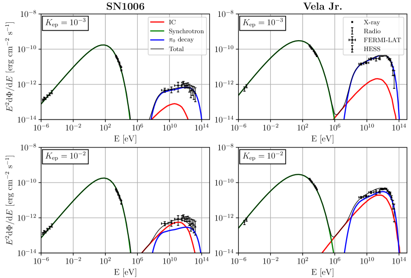
Figure 1: Multi-frequency spectra of SN1006 (left-hand panels) and Vela Jr. (right-hand panels). The top panels show a hadronic scenario for both remnants assuming an electron-to-proton ratio of $K_{\mathrm{ep}}=10^{-3}$. The bottom panels show a mixed hadronic-leptonic scenario with $K_{\mathrm{ep}}=10^{-2}$. For SN1006, we use data in the radio (Reynolds, 1996), X-rays (Bamba et al., 2008), from FERMI (Abdo et al., 2010) and H.E.S.S. (H.E.S.S. Collaboration, 2010) (sum of the two regions). For Vela Jr., we adopt data in the radio (Duncan & Green, 2000), X-rays (Aharonian et al., 2007), from FERMI (Tanaka et al., 2011) and H.E.S.S. (H.E.S.S. Collaboration, 2018b). We account for the following processes: synchrotron radiation from primary electrons (green lines), IC scattering on the CMB for SN1006 and additionally on starlight for Vela Jr. (red lines) and hadronic interactions (blue lines).

3 Multi-frequency spectral modelling

In order to improve the order of magnitude limits as presented in Sect. 2.3, we derive multi-wavelength spectra from radio to TeV gamma-rays. This enables us to carefully investigate the nature of the gamma-ray emission from both SNRs. The data are then compared to a one-zone model in which the integrated particle populations (electrons and protons, denoted by subscripts $i=\{\mathrm{e},\mathrm{p}\}$) are described by a power law with exponential cutoff of the form:

$$f^{\mathrm{1D}}(p_{i})=\dfrac{\mathrm{d}^{2}N_{i}}{\mathrm{d}p_{i}\mathrm{d}V}\propto p_{i}^{-\alpha_{i}}\exp\left[-\left(\dfrac{p_{i}}{p_{i,\mathrm{cut}}}\right)^{\beta_{i}}\right]$$ (16)

where $f^{\mathrm{1D}}(p_{i})=4\pi\,p_{i}^{2}f^{\mathrm{3D}}(p_{i})$, $\alpha_{i}$ is the spectral index, $p_{i,\mathrm{cut}}$ is the cutoff momentum and $\beta_{i}$ describes the sharpness of the cutoff; with values reported in Table 1.

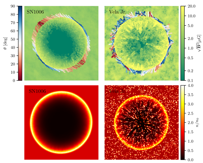
Figure 2: Two-dimensional cross-sections of our SNR simulations. Top row: slices of the magnetic field strengths of SN1006 and Vela Jr.Ḃottom row: 2D slices of the number density $n$ normalized to the background density $n_{0}$. The outwards pointing arrows in the top panels show the orientation of the magnetic field at the shock, color-coded by the magnetic obliquity (red/blue for quasi-parallel/-perpendicular shocks). Both simulation models adopt a constant-density ISM and differ only in the assumed magnetic morphology: SN1006 has a homogeneous magnetic field pointing to the top-left augmented with a mildly turbulent field while Vela Jr. adopts a fully turbulent magnetic field with correlation length $\lambda_{B}=L/2=13$ pc.

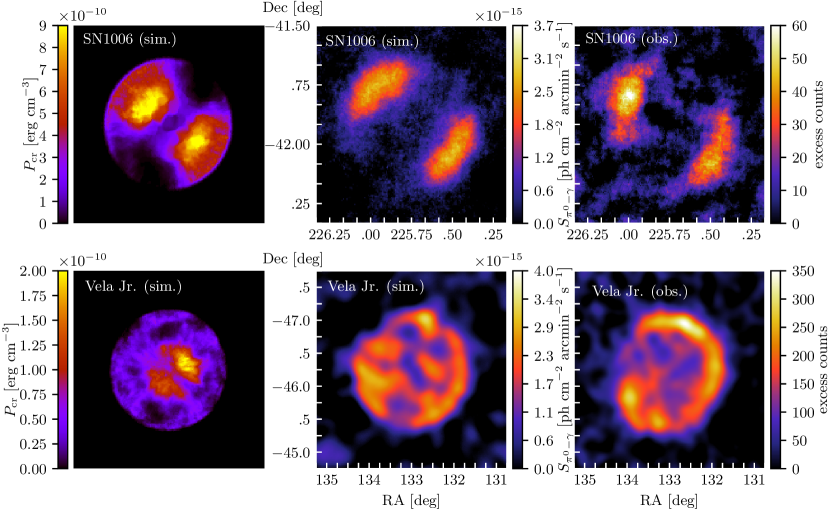
Figure 3: Two-dimensional projected gamma-ray maps of our SNR simulations. Top row, featuring SN1006: CR pressure (left), simulated pion-decay gamma-ray surface brightness resulting from hadronic CR interactions convolved to the observational resolution (middle) and acceptance-corrected excess map for SN1006 with a Gaussian PSF of width $R_{68}=0.064^{\circ}$, corresponding to $\sigma=R_{68}/1.515=0.042^{\circ}$ (H.E.S.S. Collaboration, 2010). Bottom row, featuring the same quantities for Vela Jr. with an acceptance-corrected excess map that was convolved with a Gaussian PSF of width $\sigma=0.08^{\circ}$ (H.E.S.S. Collaboration, 2018b). We add Gaussian noise at the observed level and power spectrum and convolve both simulated gamma-ray maps to the observational angular resolution.

Radio synchrotron and inverse Compton emission (including the Klein-Nishina cross section) are calculated following Blumenthal & Gould (1970). The hadronic gamma-ray emission is calculated from parametrisations of the cross-section of neutral pion production at low and high proton energies, respectively (Yang et al., 2018; Kelner et al., 2006). Because our simulations only follow CR protons, we assume an electron-to-proton ratio $K_{\mathrm{ep}}$ at 10 GeV for the normalization of the electron population. For our hadronic model we set $K_{\mathrm{ep}}=10^{-3}$. Since there are parameter degeneracies, we also show a mixed hadronic/leptonic model for the gamma-ray emission with $K_{\mathrm{ep}}=10^{-2}$.

Results for the pure hadronic and the mixed hadronic-leptonic models are shown in Fig. 1 for both SNRs. The model parameters are reported in the lower section of Tab. 1. Note that the magnetic field entering here is the radio synchrotron emission-weighted magnetic field, which is situated in the post-shock region, interior to the SNR shell. In the case of SN1006, because of its position above the galactic plane, we assume an inverse-Compton (IC) scattering mainly on CMB photons. The location of Vela Jr. in a star forming region suggests that a combination of IC scattering on starlight with an energy density of $5u_{\mathrm{CMB}}$ and CMB photons is more appropriate. In particular, we assume that the starlight is reprocessed by warm dust with a temperature of 100 K, which is typical for conditions in star forming regions (Morlino & Caprioli, 2012). Note that we adopt hard CR proton spectral indices of $\alpha_{\mathrm{p}}<2$ in all models, which naturally emerge as a result of streaming CRs inside dense clumps of a clumpy ISM (Celli et al., 2019).

4 Morphological gamma-ray modelling

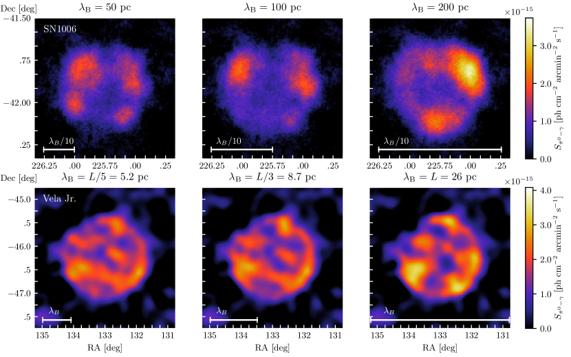
Figure 4: Synthetic gamma-ray maps of SN1006 (first row) and Vela Jr. (second row) for a purely turbulent magnetic field with different coherence lengths (see panels). The sequence towards larger correlation lengths starts to approach more homogeneous magnetic field geometries with the characteristic bi-lobed shell morphology (top right for SN1006) whereas smaller coherence lengths approach the isotropic limit (lower left for Vela Jr.). Clearly, the observed gamma-ray map of Vela Jr. falls in between the cases $\lambda_{B}=8.7$ and $26$ pc (bottom left and middle panels), justifying our choice of $\lambda_{B}=13$ pc.

Our simulation models for the two SNRs are described by the energy-conserving Sedov-Taylor solution (Ostriker & McKee, 1988). The solution also remains self similar for obliquity-dependent CR acceleration (Pais et al., 2018). We assume a power-law CR momentum distribution for calculating the pion-decay gamma-ray emissivity (Pfrommer & Enßlin, 2004; Pfrommer et al., 2008). After line-of-sight integrating the gamma-ray emissivity and adding Gaussian noise (so that the synthetic map matches the observational noise properties in amplitude and scale, see Pais & Pfrommer in prep.), we convolve the maps with the observational point-spread function.

First, we perform exploratory simulations with parameter choices guided by the self-similar scaling of the Sedov-Taylor solution. We find parameter combinations that approximately reproduce all observational characteristics (with box size $L=20$ pc for SN1006 and $L=26$ pc for Vela Jr.). Fixing angular size, explosion energy, and employing the self-similar solution, we then re-scale the solution by varying the ambient density within observational bounds to match the observed gamma-ray fluxes. In case of the core collapse supernova remnant Vela Jr. we must take into account the free expansion phase, while assuming an ejected mass of $3~{}\mathrm{M}_{\odot}$. Thus, we evolve the simulation of the Sedov explosion so that the combination of free expansion and Sedov phase matches its angular size at a given distance following Eq. (9), and we re-scale the shock radius accordingly to account for the free expansion phase. The final set of parameters is reported in Table 1.

To model SN1006 we assume a dominant homogeneous magnetic field that points to the top-left as supported by studies of radio polarization signatures (Reynoso et al., 2013). We superpose a turbulent magnetic field with a correlation length $\lambda_{B}=L=20~{}{\rm pc}$ ($\approx 0.74^{\circ}$ at $D=1.53~{}{\rm k}{\rm pc}$) that contains 1/9 of the energy density of the homogeneous field. For Vela Jr. we perform a range of fully turbulent simulations with magnetic coherence lengths $\lambda_{B}=L/f$ ($f\in\{1,2,3,4,5\}$). We find that our simulation model with $\lambda_{B}=L/2=13$ pc ($\approx 2.3^{\circ}$ at $0.5$ kpc) statistically matches the gamma-ray maps best.

We present different physical properties of our simulation models for SN1006 and Vela Jr. in Fig. 2 and 3. While both simulation models adopt a constant background density, their magnetic structure differs (Fig. 2). This results in a significantly different CR pressure distribution owing to the obliquity-dependent shock acceleration (left column of Fig. 3).

The hadronically induced gamma-ray maps echo this difference as they depend on the CR pressure distribution multiplied with the target gas density, which peaks at the shock surface (middle column of Fig. 3). The bi-lobed gamma-ray morphology of SN1006 is a direct consequence of quasi-parallel shock configuration at the polar caps. This contrasts with the patchy filamentary, limb-brightened gamma-ray morphology of our model for Vela Jr., which results from the small-scale coherent magnetic patches with a quasi-parallel shock geometry.

A direct comparison with observational images is shown in the right column of Fig. 3. In the case of SN1006, we convolve the simulated map with a Gaussian of width $\sigma=0.042^{\circ}$ (equal to $\sigma=R_{68}/1.515$ where $R_{68}=0.064^{\circ}$), in the case of Vela Jr. we use $\sigma=0.08^{\circ}$ (the observational point spread function, PSF). The obliquity-dependent shock acceleration model is able to accurately match the TeV gamma-ray morphologies of SN1006 and Vela Jr. solely by changing the magnetic coherence scale (with a homogeneous field representing the limit of an infinite coherence scale). Clearly, in the case of Vela Jr. this match is on a statistical basis as the phases of turbulent fields are random. We emphasize that all our simulations assumed a constant-density ISM that the SNR has expanded into. Note that we also obtain filamentary gamma-ray morphologies due to obliquity dependent shock acceleration in SNRs that are expanding into a stellar wind environment (see Sec. 5).

The success of our models enables us to estimate $\lambda_{B}$ of the ISM surrounding SN1006 and Vela Jr. by comparing the observed gamma-ray maps to simulations with different values of $\lambda_{B}$. While the morphology of SN1006 is best matched by a homogeneous ambient field (possibly with the addition of a small-amplitude turbulent field), we need to perform an analysis similar to Vela Jr. in order to formally place a lower limit on the magnetic coherence length. To this end, we perform three different simulations that have a purely turbulent field with coherence scales of $\lambda_{B}=50$, 100 and 200 pc. Figure 4 shows gamma-ray maps of three different magnetic coherence scales for both SNRs, respectively. For SN1006, the number of gamma-ray patches decreases with increasing coherence scale (left to right) to the point where there are two patches visible ($\lambda_{B}=200~{}{\rm pc}$). Since the alignment of these two patches is not symmetric with respect to the centre, we conclude that the true coherence scale must be larger and in fact is consistent with a nearly homogeneous field across the SNR. For Vela Jr., the sequence of gamma-ray maps with decreasing coherence scale leads to smaller-scale gamma-ray patches that asymptotically approach an isotropic distribution. We find that the correlation length of Vela Jr. ranges in between the box size $L$ and $L/3$, suggesting $\lambda_{B}\approx L/2=13_{-4.3}^{+13}$ pc, allowing for uncertainties in distance and $\lambda_{B}$.

5 SNR expanding into a stellar wind

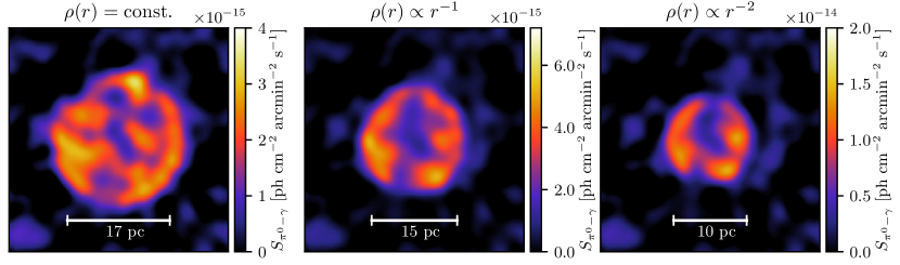
Figure 5: Synthetic $\gamma$-ray maps of Vela Jr., which result from simulations of a blast wave expanding into a stellar wind profile. To account for the uncertainties, we adopt different wind density profiles and a purely turbulent magnetic field of coherence scale $\lambda_{B}=13$ pc. The panels show SNRs that propagate in a constant density medium (left), in a density profile $\rho\propto r^{-1}$ (middle) and $\rho\propto r^{-2}$ (right) at the same age and same mean density. As expected, the higher central density slows down the expanding shock, modifies the morphology into a more compact emission region, which however maintains the shell-type morphology.

Here, we study how different assumptions of the circumstellar medium (CSM) affect the evolution of a SNR and its morphological appearance at gamma-ray energies. Studies of SNR evolution into stellar-wind-blown environments range from the initial free-expansion phase (Soderberg et al., 2010; Kamble et al., 2014; Fransson et al., 2015) to the self-similar Sedov phase (Landecker et al., 1999).

The Vela Jr. SNR is thought to be associated with a core-collapse supernova explosion (Wang & Chevalier, 2002), which results from the collapse of a massive star of mass $M\geq 8M_{\odot}$. The particularities of the progenitor are responsible for the evolution of the SNR in a highly modified wind-blown CSM shell, causing a substantially different evolution from the classical sequence of free expansion followed by a Sedov and a radiative stage (Dwarkadas, 2005). As pointed out by Chevalier (1982) and Ostriker & McKee (1988), a SNR that interacts with a CSM density profile $\rho(r)\propto r^{-q}$ has a self-similar analytical solution for the evolution of shock radius and velocity:

$$r_{\mathrm{s}}(t) =A^{\frac{1}{5-q}}t^{\frac{2}{5-q}},$$ (17)

$$v_{\mathrm{s}}(t) =\dfrac{2}{5-q}A^{\frac{1}{5-q}}t^{\frac{q-3}{5-q}},$$ (18)

where $A$ is a constant depending on the ambient average density, the SN energy and the adiabatic index. Here, $q=2$ corresponds to the case of constant mass loss from the progenitor star.

We simulate supernova explosions in three different power-law wind profiles with $q\in\{0,1,2\}$. To ease comparison we adopt the same average number density for all simulations as reported in Table 1. All other initial simulation parameters for the energy and the turbulent magnetic field remain unchanged. We evaluate the SNR simulations at the same age, which emphasizes the effect of a denser central CSM for steeper power-law indices. In order to avoid a non-vanishing magnetic divergence during the generation of the initial density profile, we cap the density in the central cells with a Plummer-type softening length of $r_{\mathrm{c}}=0.3$ pc.

The wind speed $v_{w}$ ranges from values of order $(1000-3000)~{}{\rm k}{\rm m}\ {\rm s}^{-1}$ for very young SNRs (Abbott, 1978) to $100\ {\rm k}{\rm m}\ {\rm s}^{-1}$ or less for red-giant stars. Hence, we can neglect $v_{w}$ in comparison to the shock velocity during the early Sedov phase (Ostriker & McKee, 1988), which means that the approximation of assuming a point explosion in the various density profiles is fully justified and does not affect the final simulation result. This causes the remnant to directly enter the Sedov stage and to bypass the earlier phase of a swept-up wind-blown shell.

In Fig. 5 we show simulated gamma-ray maps of Vela Jr. for the three different CSM environments. The primary effect of a stratified wind density profile consists of slowing down the propagating blast wave. This results in a more compact and brighter gamma-ray morphology. Many of the general morphological features of the patchy gamma-ray map previously found for the constant density solution carry over to the stratified density profiles. However, the higher central number density in comparison to the flat profile increases the gamma-ray brightness, with a flux enhancement by a factor of six for the $q=2$ profile, as expected for the evolution of these profiles at early times (Kirk et al., 1995). Thus, comparing our simulated maps to the observed shell-type morphologies at these ages, this argues for more shallow density profiles $|q|<1$, with slight preferences for a constant density medium for the SNRs studied here.

6 Discussion and Conclusions

We have presented the first global simulations and gamma-ray maps of SNRs in the hadronic model, which account for magnetic obliquity-dependent CR acceleration. We show that the multi-frequency spectrum in the hadronic and mixed hadronic/leptonic models match observational data for our simulation parameters of the ISM, which are motivated by observations. Our synthetic gamma-ray maps match the apparently disparate TeV morphologies and total gamma-ray fluxes of SNR 1006 and Vela Jr. within a single physical model extremely well: SN1006 expands into a homogeneous magnetic field that is reminiscent of conditions for a galactic outflow or a large-scale Parker loop as supported by its Galactic height of $z=0.6$ kpc (at $D\simeq 1.8~{}$kpc) above the midplane (Stephenson & Green, 2002). On the contrary, Vela Jr. is embedded in a small-scale turbulent field typical of spiral arms. This suggests that the diversity of shell-type TeV SNRs originates in the obliquity dependence of the acceleration process rather than in density inhomogeneities.

Comparing our simulations of different $\lambda_{B}$ to observed TeV maps of shell-type SNRs enables us to estimate $\lambda_{B}$ of the unperturbed ISM before it encountered the SNR blast wave. Assuming statistical homogeneity, we constrain $\lambda_{B}$ in the vicinity of SN1006 and Vela Jr. to $>200_{-10}^{+80}$ pc and $13_{-4.3}^{+13}$ pc, respectively. Simulating the SN explosion that expands into a stratified density profile caused by a stellar wind produces similarly patchy gamma-ray maps and hence does not alter our conclusions that magnetic obliquity-dependent CR acceleration is responsible for this patchy morphology. However, at the same mean density, the blast wave will encounter a denser CSM at small radii, which slows down the propagating blast wave and results in a more compact and brighter gamma-ray map at the same age.

If obliquity-dependent diffusive shock acceleration also applies to electrons, we could produce similar synthetic TeV maps in the leptonic model to constrain the magnetic coherence length. If electron acceleration were independent of magnetic obliquity then this work would provide strong evidence for the hadronic scenario in shell-type SNRs as the necessary element to explain the patchy TeV emission. In any case, we conclude that the inferred coherence scales are robust to specific assumptions of the gamma-ray emission scenario (hadronic vs. leptonic models).

Moreover, here we show that the hadronic model is able to explain shell-type SNR morphologies, which naturally emerge in our simulations due to the peaked density at the shock in combination with the slowly decreasing CR pressure profile (Pais et al., 2018). In the leptonic model, fast electron cooling would have to confine the emission regions close to the shock. However, this would imply strong spectral softening towards the SNR interior, which is not observed in Vela Jr., seriously questioning the leptonic model for this SNR (H.E.S.S. Collaboration, 2018b). Our work opens up the possibility of mapping out the magnetic coherence scale across the Milky Way and other nearby galaxies at the locations of TeV shell-type SNRs, and to study how it varies depending on its vertical height or its location with respect to a spiral arm. Thus, our work represents an exciting new science case for gamma-ray astronomy, in particular for the Cherenkov Telescope Array.

Appendix A Analytical model for the gamma-ray luminosity in a clumped medium

Here, we study the interaction of a shock with a dense cloud with numerical simuations and analytics and construct an analytical model for the gamma-ray luminosity from a core collapse SNR. We assume that the shock propagates through a highly structured ISM with a large population of dense clouds, which plays an important role for the resulting multi-frequency emission (Wang & Chevalier, 2002).

A.1 Numerical setup

To capture the clumpy structure of the ISM in these regions we generated $7\times 10^{3}$ dense gaseous clumps with a radius of $R_{\mathrm{c}}=0.05~{}{\rm pc}$ each and uniformly distributed in a box of size $L=25~{}{\rm pc}$, subset of the simulation box of size $L=26~{}{\rm pc}$. We used a margin of $0.5~{}{\rm pc}$ for each side of the cube to avoid any incidental misplacement of the clumps. We deposit a total mass of dense clumps of $M^{\mathrm{tot}}_{\mathrm{c}}=255~{}M_{\odot}$ within the selected box so that each clump has a mass of $M_{\mathrm{c}}=0.036~{}M_{\odot}$ and the volume-averaged $\mathrm{H}_{2}$ density is $\langle\rho_{\mathrm{c}}\rangle=1.6\times 10^{-2}~{}M_{\odot}{\rm pc}^{-3}$. Following a setup similar to Celli et al. (2019), we assume spherical clumps with a number density $n_{\mathrm{c}}=1.4\times 10^{3}~{}{\rm c}{\rm m}^{-3}$ and a molecular weight $\mu=2$ (associated to the clumps) so that the density contrast with respect to the background is $\delta=n_{\mathrm{c}}/n_{0}\sim 3\times 10^{3}$. Note that we neglect radiative cooling in these simulations, which is negligible over the propagation time of the SNR shocks considered while it is crucial for understanding the (thermo-)dynamics of the system on longer time scales (McCourt et al., 2018; Gronke & Oh, 2018; Sparre et al., 2019).

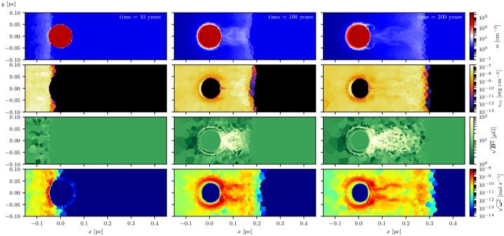
Figure 6: Snapshots of the shock-cloud interaction at $t=10,100$ and $200$ yrs after the collision for a density contrast of $\delta=10^{3}$. For each time we show slices of the gas density (top row), CR energy density (second row), magnetic field strength (third row) and magnitude of the vorticity (fourth row).

We use the code AREPO, which employs an unstructured mesh that is defined as the Voronoi tessellation of a set of mesh-generating points. If they move with the local fluid speed, the scheme inherits the advantages of Lagrangian fluid methods that keep the mass per cell approximately fixed. AREPO allows for super-Lagrangian resolution capabilities by inserting new mesh points. Hence, in order to accurately describe the dynamics of the dense clouds, each small clump is resolved with $10^{3}$ cells that are uniformly distributed within a spherical volume. To ensure a smooth transition between the larger cell size in the low-density diffuse ISM and the well-resolved clumps, we initially place a buffer shell of thickness $0.01~{}{\rm pc}$ with the density of the diffuse ISM and the high resolution of the clump cells. Despite the high post-shock vorticity caused by the impact of shock front on the clumps, the volume fraction occupied by the dense bullets is small enough to maintain the shock front practically self similar throughout its evolution in the medium.

A.2 Interaction of a shock with a dense clump

Because of momentum conservation, the SNR shock penetrates much slower in the dense clump in comparison to the shock velocity in the dilute medium outside the clump and thus, only a fraction of dense gas inside these objects is accelerated at a given time. To investigate the mass fraction $\eta$ that is processed by the shock, we conduct simulations with clumps of different density ($n_{\mathrm{c}}=\{10^{2},10^{3},10^{4}\}~{}{\rm c}{\rm m}^{-3}$). To accurately describe the dynamics, we resolve the cloud with $1.5\times 10^{5}$ particles within a radius of $0.05~{}{\rm pc}$. We place the cloud in a shock-tube of length $2~{}{\rm pc}$ and density of $n_{0}=1~{}{\rm c}{\rm m}^{-3}$. The shock is set to propagate in the $x$ direction with initial density and pressure jumps so that the initial shock velocity is $v_{\mathrm{s}}=5000~{}{\rm k}{\rm m}~{}{\rm s}^{-1}$. Different snapshots of the shock-cloud interaction for a density contrast of $\delta=10^{3}$ are reported in Fig. 6.

When the supernova blast wave impacts a dense structure at some constant (oblique) angle, it experiences the same “shock deflection” and amount of entropy injection along the shock front because only the parallel velocity component is reduced by the compression ratio while the perpendicular component is conserved. If the blast wave encounters a dense, curved structure, the incoming velocity experiences a different amount of deflection along the shock surface (perpendicular to the shock normal), which injects voriticty according to Crocco’s theorem (1937). This vorticity is injected at the length scale of the clump and cascades to smaller scales with increasing distance from the shock. The shock in the dilute phase closes in after passing the clump and eventually straightens up as it closes the dip at the location of the clump after about 100 years (see Fig. 6). While the shock front propagates seemingly undisturbed at larger distances from the clump, it has dramatically slowed down inside the clump as a result of momentum conservation. The relic of such a complex history of the shock evolution is a highly turbulent tail in the downstream of the clump, which is able to drive a small-scale turbulent dynamo that amplifies the magnetic field there. This behavior is consistent with the lower resolution simulation of the entire SNR presented in top right panel of Fig. 2, where a system of uniformly distributed clumps leave several magnetized finger-like structures after the collision with the blast wave.

The interaction of a shock with a spherical object has been previously studied by Pfrommer & Jones (2011) for a low-density bubble, the results of which can also be applied to the case of a dense clump by exchanging the rarefaction wave with a reverse shock characteristics that propagates in the opposite direction of the original shock. Solving the Riemann problem in this case, we can relate the initial shock speed $v_{\mathrm{s0}}$ in the dilute phase to the shock speed $v_{\mathrm{sc}}$ propagating inside the clump. The dilute and the clump phases have the same initial pressure $P_{0}$ while the sound speeds of the dense and dilute media are related by $c_{\mathrm{c}}=\sqrt{\gamma P_{0}/\rho_{\mathrm{c}}}=c_{0}/\sqrt{\delta}$. The equation for a left reverse shock condition (Toro, 2009) reads:

$$v_{\ast}=v_{\mathrm{L}}+(P_{\mathrm{L}}-P_{\ast})\sqrt{\dfrac{2}{\gamma_{\mathrm{L}}+1}}\left[\rho_{\mathrm{L}}\left(P_{\ast}+\dfrac{\gamma_{\mathrm{L}}-1}{\gamma_{\mathrm{L}}+1}P_{\mathrm{L}}\right)\right]^{-1/2}$$ (19)

where the subscript “$\ast$” denotes the state behind the reverse shock while the subscript L represents the state ahead of the reverse shock. Introducing the Mach number ratio $\mu=\mathcal{M}_{\mathrm{c}}/\mathcal{M}_{0}=\sqrt{\delta}\,v_{\mathrm{sc}}/v_{\mathrm{s0}}$, assuming $\gamma_{0}=\gamma_{\mathrm{c}}=5/3$, and combining the various jump conditions (see eq. (B1) in Appendix B of Pfrommer & Jones 2011 with subscript $\mathrm{L}=3$) we find an equation for $\mu$ as a function of the Mach number $\mathcal{M}_{0}$ in the dilute phase and the density contrast $\delta$:

$$1= \sqrt{\delta}\mu-\mu\mathcal{M}_{0}^{2}\left(\sqrt{\delta}-\mu\right)$$ (20)

$$+\mu\left(\mu^{2}-1\right)\mathcal{M}_{0}^{2}\sqrt{\frac{\delta\left(\mathcal{M}_{0}^{2}+3\right)}{\left(4\mu^{2}+1\right)\mathcal{M}_{0}^{2}-1}},$$

which has a numerical solution for $\mu$ given $\mathcal{M}_{0}$ and $\delta$. In the regime of strong shocks (i.e., $\mathcal{M}_{0}\gg 1$) Eq. (20) is reduced to the simpler form:

$$\mu=(1-\mu^{2})\sqrt{\frac{\delta}{4\mu^{2}+1}}+\sqrt{\delta}$$ (21)

For $\delta\gg 1$ Eq. (21) can be easily solved and has the positive root $\mu=\sqrt{6}$. In order to account for multi-dimensional effects of order unity, we introduce a factor $f_{\mathrm{d}}$ that we calibrate on our three-dimensional (3D) simulations and write the solutions as $\mu=f_{\mathrm{d}}\sqrt{6}$. Because $\mu=\sqrt{\delta}\,v_{\mathrm{sc}}/v_{\mathrm{s0}}$ we conclude that $v_{\mathrm{sc}}\propto\delta^{-1/2}v_{\mathrm{s0}}$. We confirm the applicability of this scaling behavior in 3D simulations by fitting the appropriate power law to the shock tube simulation of the three different density contrasts (see Fig. 7). The theoretically expected scaling matches the simulations within the variance of the shock velocity, however the pre-factor found in our 3D simulations is closer to 1.2 rather than 2, which means that $f_{\mathrm{d}}\simeq 1/2$. A comparison between 1D runs and 3D runs for density contrasts of $10^{2}$, $10^{3}$ and $10^{4}$ is shown in Fig. 8. In the following formulas to construct the analytical model for the gamma-ray luminosity we will apply the 3D pre-factor rather than the 1D prediction.

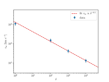
Figure 7: Simulated shock velocity $v_{\mathrm{sc}}$ inside a dense clump as a function of the density contrast for the cases $\delta=[10^{2},10^{3},10^{4}]$. The point for $\delta=1$ represents the shock velocity in the dilute phase. Within the uncertainty, the simulation points follow the $\delta^{-1/2}$ scaling behaviour derived in Eq. (21).

A.3 Constructing the analytical model

To calculate the mass fraction of the clump that is processed by the shock, we proceed as follows. We follow the shock-wave propagation inside the clump and calculate the amount of shocked gas inside the clump as a function of time. We define the shock-processed clump mass fraction $\eta(t)$ as the ratio between the shocked gas mass of the dense clump and its total mass as a function of time.

A shock propagates in a shock-tube with the velocity $\propto t^{-1/3}$ as predicted by the 1D Sedov problem while a 3D blast wave evolves according to $t^{-3/5}$. In the latter case we integrate the velocity to obtain the shock propagation length inside the clump as a function of time:

$$r(t,t_{0}) =f_{\mathrm{d}}\sqrt{\frac{6}{\delta}}\int_{t_{0}}^{t}v_{\mathrm{s0}}(t^{\prime})\mathrm{d}t^{\prime}$$ (22)

$$=f_{\mathrm{d}}\sqrt{\frac{6}{\delta}}\left(\dfrac{E_{\mathrm{SN}}}{\alpha\rho_{0}}\right)^{1/5}[t^{2/5}-t_{0}^{2/5}]$$

which is valid for $t_{0}<t<t_{\mathrm{c}}(t_{0})$, where $t_{0}$ is the time of the supernova shock impacting the clump and $t_{\mathrm{c}}$ is the crossing time of the shock inside the clump, which can be obtained from the requirement that the shock propagation length has to be smaller than the size of the clump,

$$t_{\mathrm{c}}(t_{0})=\left[\dfrac{2R_{\mathrm{c}}}{f_{\mathrm{d}}\sqrt{6}}\delta^{1/2}\left(\dfrac{E_{\mathrm{SN}}}{\alpha\rho_{0}}\right)^{-1/5}+t_{0}^{2/5}\right]^{5/2}.$$ (23)

This means that for typical values, the shock propagation length in the clump is

$$r(t,t_{0})=0.064~{}{\rm pc}~{}\left(\frac{\delta}{10^{3}}\right)^{-1/2}\left(\dfrac{n}{0.1~{}{\rm c}{\rm m}^{-3}}\right)^{-1/5}$$ (24)

for $t=1~{}{\rm kyr}$ and $t_{0}=500~{}{\rm yr}$. We can determine the volume of the shocked material inside the clump using Eq. (22) as the height of a polar cap as a function of time, while neglecting the curvature of the shock inside the clump. The ratio between the shocked polar cap volume of the clump and its total volume reads

$$\eta(t,t_{0})=\dfrac{V_{\mathrm{cap}}}{V_{\mathrm{tot}}}=\dfrac{\pi/3\times r^{2}(3R_{\mathrm{c}}-r)}{4\pi/3\times R^{3}_{\mathrm{c}}}=\dfrac{r^{2}(3R_{\mathrm{c}}-r)}{4R^{3}_{\mathrm{c}}},$$ (25)

where $r=r(t,t_{0})$ and we used the fact that the clump density is constant. Eq. (25) represents the mass fraction accelerated by the shock as a function of time. For $r(t,t_{0})=2R_{\mathrm{c}}$ we set $\eta(t,t_{0})=0$ to indicate that the clump is either destroyed by MHD instabilities or emptied of CRs.

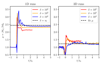
Figure 8: Mach number ratio evolution after the interaction with a dense region for various density contrasts. Left: the 1D shocktube runs show a good agreement with the theoretical value reported in Eq. (21) (dashed line). Right: the 3D runs show a lower pre-factor with respect to the 1D theoretical estimate. The case with $\delta=10^{2}$ is interrupted in both case by the finite size of the clumpy region.

Assuming that a uniform spatial distribution of clumps is overrun by a self-similar quasi-spherical blast wave, it is clear that the shock interacts at different times with individual clumps. This implies that the innermost clumps close to the explosion site have a higher fraction of shocked mass in comparison to clumps at the periphery. For this reason we have to weight Eq. (25) with a distribution of clumps that interact with the shock per unit time. Assuming that the number of clumps is large so that the continuum limit applies, the number of clumps that start to interact with the SNR shock is given by

$$\dot{N}(t) =\dfrac{\mathrm{d}N(t)}{\mathrm{d}t}=\dfrac{\langle\rho_{c}\rangle}{M_{\mathrm{c}}}\dfrac{\mathrm{d}V_{s}(t)}{\mathrm{d}t}=\dfrac{4}{3}\pi\dfrac{\langle\rho_{c}\rangle}{M_{\mathrm{c}}}\dfrac{\mathrm{d}[r_{s}^{3}(t)]}{\mathrm{d}t}$$ (26)

$$=\dfrac{1.7}{{\rm yr}}\left(\dfrac{t}{1~{}{\rm kyr}}\right)^{1/5}\left(\dfrac{\langle\rho_{c}\rangle}{M_{\odot}{\rm pc}^{-3}}\right)\left(\dfrac{M_{\mathrm{c}}}{M_{\odot}}\right)^{-1}$$

In the last step, we assume the Sedov-Taylor regime for the SNR because the fraction of volume swept-up in the free expansion phase is only about $0.3\%$ of the final volume and it encompasses only less than $20$ clumps for our setup. Using Eqs. (25) and (26) the average efficiency $\eta(t)$ weighted by the number of interacting clumps per unit time for a SNR reads

$$\bar{\eta}(t) =\dfrac{\displaystyle\int_{0}^{t}\dot{N}(t^{\prime})\eta(t,t^{\prime})\mathrm{d}t^{\prime}}{\displaystyle\int_{0}^{t}\dot{N}(t^{\prime})\mathrm{d}t^{\prime}}$$ (27)

$$\simeq\left\{\dfrac{1}{52\tilde{r}^{9/4}(t,\delta,n)}+7\tilde{r}^{2/3}(t,\delta,n)\right\}^{-1},$$

where

$$\tilde{r}(t,\delta,n)=0.25\left(\dfrac{\delta}{10^{3}}\right)^{-1/2}\left(\dfrac{n}{0.1~{}{\rm c}{\rm m}^{-3}}\right)^{-1/5}\left(\dfrac{t}{1~{}{\rm kyr}}\right)^{2/5}.$$ (28)

Results for different values of $\delta$ are plotted in Fig. 9. For $\delta=3\times 10^{3}$ and $t=2.5~{}{\rm kyr}$ we find $\eta(t)\simeq 32\%$, which is slightly higher than the value found in the simulation (around $30\%$).

Figure 9: Evolution of $\bar{\eta}(t)$ for different values of $\delta=3\times[10^{2},10^{3},10^{4}]$ for $n=0.42~{}{\rm c}{\rm m}^{-3}$. The lines represent the theoretical values calculated via Eq. (27). Although an increasing number of clumps are hit by the shock the slowdown of the blast wave transfers a decreasing amount of momentum to the clumps leading to an ideal asymptotic value for $\bar{\eta}(t)$. The dashed lines represent the case where the clumps are not destroyed and continue to be active sources of CRs.

To obtain the gamma-ray luminosity $\mathcal{L}_{\gamma}=4\pi D^{2}\mathcal{F}_{\gamma}$ due to hadronic CR proton interactions, we separately calculate the contributions from the dilute phase and the clouds and then add them together:

$$\mathcal{L}_{\gamma}=\int s_{\pi^{0}\rightarrow\gamma}\mathrm{d}V=\mathcal{L}_{\gamma,\mathrm{d}}+\mathcal{L}_{\gamma,\mathrm{c}},$$ (29)

where $s_{\pi^{0}\rightarrow\gamma}$ is the neutral pion-decay source function (Pfrommer & Enßlin, 2004). The contribution from the dilute phase is given by

$$\mathcal{L}_{\gamma,\mathrm{d}}=5.3\times 10^{32}\left(\dfrac{W_{\mathrm{p}}}{10^{50}~{}{\rm erg}}\right)\left(\dfrac{\langle n\rangle}{0.1~{}{\rm c}{\rm m}^{-3}}\right)\dfrac{\mathrm{ph}}{{\rm s}},$$ (30)

where $W_{\mathrm{p}}$ the total proton energy integrated over the whole SNR volume and $\langle n\rangle$ is the volume averaged number density, which approximately coincides with the number density on the dilute phase due to the negligible volume filling factor of the dense clumps, $f_{V}=V_{\mathrm{c}}/V=2.4\times 10^{-4}$ for our parameters. The gamma-ray luminosity associated to the clumped gas is:

$$\mathcal{L}_{\gamma,\mathrm{c}}=\int s_{\pi^{0}\rightarrow\gamma}\mathrm{d}V_{\mathrm{c}}=\int s_{\pi^{0}\rightarrow\gamma}f_{V}\mathrm{d}V$$ (31)

$$=1.6\times 10^{32}\left(\dfrac{\bar{\eta}(t)}{30\%}\right)\left(\dfrac{f_{V}}{10^{-4}}\right)\left(\dfrac{n_{\mathrm{c}}}{10^{3}~{}{\rm c}{\rm m}^{-3}}\right)\left(\dfrac{W_{\mathrm{p}}}{10^{50}~{}{\rm erg}}\right)\dfrac{\mathrm{ph}}{{\rm s}}$$

where $V_{\mathrm{c}}$ is the volume occupied by the clumps and $\bar{\eta}(t)$ is the average fraction of the shocked clump volume fraction inside the remnant volume. In our setup we set $n_{\mathrm{c}}=1.4\times 10^{3}{\rm c}{\rm m}^{-3}$. Combining Eqs. (30) and (31) we get

$$\mathcal{L}_{\gamma} =\mathcal{L}_{\gamma,\mathrm{s}}+\mathcal{L}_{\gamma,\mathrm{c}}$$ (32)

$$=5.3\times 10^{32}(1+\chi)\left(\dfrac{W_{\mathrm{p}}}{10^{50}~{}{\rm erg}}\right)\left(\dfrac{n}{0.1~{}{\rm c}{\rm m}^{-3}}\right)\dfrac{\mathrm{ph}}{{\rm s}}$$

where

$$\chi=0.3\left(\dfrac{\bar{\eta}(t)}{30\%}\right)\left(\dfrac{f_{V}}{10^{-4}}\right)\left(\dfrac{n_{\mathrm{c}}}{10^{3}~{}{\rm c}{\rm m}^{-3}}\right)\left(\dfrac{n}{0.1~{}{\rm c}{\rm m}^{-3}}\right)^{-1}.$$ (33)

It is easy to verify that Eq. (12) is equivalent to Eq. (33) because of the following identity:

$$f_{V}n_{\mathrm{c}}=\dfrac{f_{V}\rho_{\mathrm{c}}}{\mu_{\mathrm{H}}m_{\mathrm{p}}}=\dfrac{\langle\rho_{\mathrm{c}}\rangle}{\mu_{\mathrm{H}}m_{\mathrm{p}}}$$ (34)

In terms of normalized quantities the previous equation becomes:

$$\left(\dfrac{f_{V}}{2.4\times 10^{-4}}\right)\left(\dfrac{n_{\mathrm{c}}}{1.4\times 10^{3}~{}{\rm c}{\rm m}^{-3}}\right)=\left(\dfrac{\langle\rho_{\mathrm{c}}\rangle}{1.6\times 10^{-2}M_{\odot}{\rm pc}^{-3}}\right).$$ (35)

References

- Abbott (1978) Abbott D. C., 1978, ApJ, 225, 893
- Abdo et al. (2010) Abdo A. A., et al., 2010, Astrophys. J. Suppl. Ser., 188, 405
- Acero et al. (2007) Acero F., Ballet J., Decourchelle A., 2007, Astron. Astrophys., 475, 883
- Acero et al. (2015) Acero F., Lemoine-Goumard M., Renaud M., Ballet J., Hewitt J. W., Rousseau R., Tanaka T., 2015, Astron. Astrophys., 580, A74
- Ackermann et al. (2013) Ackermann et al. M., 2013, Science, 339, 807
- Aharonian et al. (2006) Aharonian et al. F., 2006, Astron. Astrophys., 449, 223
- Aharonian et al. (2007) Aharonian et al. F., 2007, ApJ, 661, 236
- Allen et al. (2015) Allen G. E., Chow K., DeLaney T., Filipović M. D., Houck J. C., Pannuti T. G., Stage M. D., 2015, ApJ, 798, 82
- Araya & Frutos (2012) Araya M., Frutos F., 2012, Mon. Not. R. Astron. Soc., 425, 2810
- Archambault et al. (2017) Archambault et al. S., 2017, ApJ, 836, 23
- Aschenbach et al. (1999) Aschenbach B., Iyudin A. F., Schönfelder V., 1999, Astron. Astrophys., 350, 997
- Atoyan et al. (2000) Atoyan A. M., Aharonian F. A., Tuffs R. J., Völk H. J., 2000, Astron. Astrophys., 355, 211
- Bamba et al. (2008) Bamba et al. A., 2008, Publications of the Astronomical Society of Japan, 60, S153
- Bell (1978) Bell A. R., 1978, Mon. Not. R. Astron. Soc., 182, 147
- Bell (2004) Bell A. R., 2004, Mon. Not. R. Astron. Soc., 353, 550
- Berezhko & Völk (2008) Berezhko E. G., Völk H. J., 2008, Astron. Astrophys., 492, 695
- Blandford & Ostriker (1978) Blandford R. D., Ostriker J. P., 1978, Astrophys. J. Lett., 221, L29
- Blumenthal & Gould (1970) Blumenthal G. R., Gould R. J., 1970, Reviews of Modern Physics, 42, 237
- Caprioli & Spitkovski (2014) Caprioli D., Spitkovski A., 2014, ApJ, 783, 91
- Cardillo et al. (2016) Cardillo M., Amato E., Blasi P., 2016, Astron. Astrophys., 595, A58
- Celli et al. (2019) Celli S., Morlino G., Gabici S., Aharonian F. A., 2019, Mon. Not. R. Astron. Soc., 487, 3199
- Chevalier (1982) Chevalier R. A., 1982, ApJ, 258, 790
- Crocco (1937) Crocco L., 1937, Zeitschrift Angewandte Mathematik und Mechanik, 17, 1
- Dubner et al. (2002) Dubner G. M., Giacani E. B., Goss W. M., Green A. J., Nyman L. Å., 2002, Astron. Astrophys., 387, 1047
- Duncan & Green (2000) Duncan A. R., Green D. A., 2000, Astron. Astrophys., 364, 732
- Dwarkadas (2005) Dwarkadas V. V., 2005, ApJ, 630, 892
- Fransson et al. (2015) Fransson et al. C., 2015, Astrophys. J. Lett., 806, L19
- Fukui (2013) Fukui Y., 2013, in Torres D. F., Reimer O., eds, Astrophysics and Space Science Proceedings Vol. 34, Cosmic Rays in Star-Forming Environments. p. 249 (arXiv:1304.1261), doi:10.1007/978-3-642-35410-6˙17
- Fukui & Sano et al. (2017) Fukui Y., Sano et al. H., 2017, ApJ, 850, 71
- Gabici & Aharonian (2014) Gabici S., Aharonian F. A., 2014, Mon. Not. R. Astron. Soc., 445, L70
- Gabici & Aharonian (2016) Gabici S., Aharonian F., 2016, in European Physical Journal Web of Conferences. p. 04001, doi:10.1051/epjconf/201612104001
- Giacalone et al. (1992) Giacalone J., Burgess D., Schwartz S. J., Ellison D. C., 1992, Geophys. Res. Lett., 19, 433
- Goldreich & Sridhar (1995) Goldreich P., Sridhar S., 1995, ApJ, 438, 763
- Green (2014) Green D. A., 2014, Bulletin of the Astronomical Society of India, 42, 47
- Gronke & Oh (2018) Gronke M., Oh S. P., 2018, Mon. Not. R. Astron. Soc., 480, L111
- H.E.S.S. Collaboration (2010) H.E.S.S. Collaboration 2010, Astron. Astrophys., 516, A62
- H.E.S.S. Collaboration (2018a) H.E.S.S. Collaboration 2018a, Astron. Astrophys., 612, A6
- H.E.S.S. Collaboration (2018b) H.E.S.S. Collaboration 2018b, Astron. Astrophys., 612, A7
- Hinton & Hofmann (2009) Hinton J. A., Hofmann W., 2009, ARA&A, 47, 523
- Inoue et al. (2012) Inoue T., Yamazaki R., Inutsuka S.-i., Fukui Y., 2012, ApJ, 744, 71
- Iyudin et al. (1998) Iyudin et al. A., 1998, Nature, 396, 142
- Ji et al. (2016) Ji S., Oh S. P., Ruszkowski M., Markevitch M., 2016, Mon. Not. R. Astron. Soc., 463, 3989
- Kamble et al. (2014) Kamble et al. A., 2014, ApJ, 797, 2
- Katsuda (2017) Katsuda S., 2017, Supernova of 1006 (G327.6+14.6). (arXiv:1702.02054), doi:10.1007/978-3-319-21846-5˙45
- Katsuda et al. (2008) Katsuda S., Tsunemi H., Mori K., 2008, Astrophys. J. Lett., 678, L35
- Katsuda et al. (2009) Katsuda S., Petre R., Long K. S., Reynolds S. P., Winkler P. F., Mori K., Tsunemi H., 2009, Astrophys. J. Lett., 692, L105
- Kelner et al. (2006) Kelner S. R., Aharonian F. A., Bugayov V. V., 2006, Phys. Rev. D, 74, 034018
- Kirk et al. (1995) Kirk J. G., Duffy P., Ball L., 1995, Astron. Astrophys., 293
- Landecker et al. (1999) Landecker T. L., Routledge D., Reynolds S. P., Smegal R. J., Borkowski K. J., Seward F. D., 1999, ApJ, 527, 866
- Lloyd (1982) Lloyd S. P., 1982, IEEE Trans. Information Theory, 28, 129
- Long et al. (2003) Long K. S., Reynolds S. P., Raymond J. C., Winkler P. F., Dyer K. K., Petre R., 2003, ApJ, 586, 1162
- Maxted et al. (2018) Maxted N. I., et al., 2018, ApJ, 866, 76
- McCourt et al. (2018) McCourt M., Oh S. P., O’Leary R., Madigan A.-M., 2018, Mon. Not. R. Astron. Soc., 473, 5407
- McKee & Ostriker (1977) McKee C. F., Ostriker J. P., 1977, ApJ, 218, 148
- Ming et al. (2019) Ming J., et al., 2019, Phys. Rev. D, 100, 024063
- Morlino & Caprioli (2012) Morlino G., Caprioli D., 2012, Astron. Astrophys., 538, A81
- Ostriker & McKee (1988) Ostriker J. P., McKee C. F., 1988, Reviews of Modern Physics, 60, 1
- Pais et al. (2018) Pais M., Pfrommer C., Ehlert K., Pakmor R., 2018, Mon. Not. R. Astron. Soc., 478, 5278
- Pakmor & Springel (2013) Pakmor R., Springel V., 2013, Mon. Not. R. Astron. Soc., 432, 176
- Pakmor et al. (2016) Pakmor R., Springel V., Bauer A., Mocz P., Munoz D. J., Ohlmann S. T., Schaal K., Zhu C., 2016, Mon. Not. R. Astron. Soc., 455, 1134
- Petruk et al. (2011) Petruk O., Beshley V., Bocchino F., Miceli M., Orlando S., 2011, Mon. Not. R. Astron. Soc., 413, 1643
- Pfrommer & Enßlin (2004) Pfrommer C., Enßlin T. A., 2004, Astron. Astrophys., 413, 17
- Pfrommer & Jones (2011) Pfrommer C., Jones T. W., 2011, ApJ, 730, 22
- Pfrommer et al. (2008) Pfrommer C., Enßlin T. A., Springel V., 2008, Mon. Not. R. Astron. Soc., 385, 1211
- Pfrommer et al. (2017) Pfrommer et al. C., 2017, Mon. Not. R. Astron. Soc., 465, 4500
- Pohl (1996) Pohl M., 1996, Astron. Astrophys., 307, L57
- Powell et al. (1999) Powell K. G., Roe P. L., Linde T. J., Gombosi T. I., De Zeeuw D. L., 1999, J. Comput. Phys., 154, 284
- Reynolds (1996) Reynolds S. P., 1996, ApJ, 459, L13
- Reynoso et al. (2013) Reynoso E. M., Hughes J. P., Moffett D. A., 2013, Astronom. J., 145, 104
- Schaal & Springel (2015) Schaal K., Springel V., 2015, Mon. Not. R. Astron. Soc., 446, 3992
- Sedov (1959) Sedov L. I., 1959, Similarity and Dimensional Methods in Mechanics
- Slane et al. (2001) Slane P., Hughes J. P., Edgar R. J., Plucinsky P. P., Miyata E., Tsunemi H., Aschenbach B., 2001, ApJ, 548, 814
- Soderberg et al. (2010) Soderberg A. M., Brunthaler A., Nakar E., Chevalier R. A., Bietenholz M. F., 2010, ApJ, 725, 922
- Sparre et al. (2019) Sparre M., Pfrommer C., Vogelsberger M., 2019, Mon. Not. R. Astron. Soc., 482, 5401
- Springel (2010) Springel V., 2010, Mon. Not. R. Astron. Soc., 401, 791
- Stage et al. (2006) Stage M. D., Allen G. E., Houck J. C., Davis J. E., 2006, Nature Physics, 2, 614
- Stephenson & Green (2002) Stephenson F. R., Green D. A., 2002, Historical supernovae and their remnants, by F. Richard Stephenson and David A. Green. International series in astronomy and astrophysics, vol. 5. Oxford: Clarendon Press, 2002, ISBN 0198507666, 5
- Tanaka et al. (2011) Tanaka T., et al., 2011, Astrophys. J. Lett., 740, L51
- Telezhinsky (2009) Telezhinsky I., 2009, Astroparticle Physics, 31, 431
- Toro (2009) Toro E., 2009, Riemann Solvers and Numerical Methods for Fluid Dynamics: A Practical Introduction, doi:10.1007/b79761.
- Truelove & McKee (1999) Truelove J. K., McKee C. F., 1999, Astrophys. J. Suppl. Ser., 120, 299
- Uchiyama et al. (2007) Uchiyama Y., Aharonian F. A., Tanaka T., Takahashi T., Maeda Y., 2007, Nature, 449, 576
- Wang & Chevalier (2001) Wang C.-Y., Chevalier R. A., 2001, ApJ, 549, 1119
- Wang & Chevalier (2002) Wang C.-Y., Chevalier R. A., 2002, ApJ, 574, 155
- Winkler et al. (2003) Winkler P. F., Gupta G., Long K. S., 2003, ApJ, 585, 324
- Xing et al. (2016) Xing Y., Wang Z., Zhang X., Chen Y., 2016, ApJ, 823, 44
- Yang et al. (2018) Yang R.-z., Kafexhiu E., Aharonian F., 2018, preprint, (arXiv:1803.05072)
- Zirakashvili & Aharonian (2010) Zirakashvili V. N., Aharonian F. A., 2010, ApJ, 708, 965