Cm-wavelength observations of MWC 758: resolved dust trapping in a vortex

Abstract

The large crescents imaged by ALMA in transition disks suggest that azimuthal dust trapping concentrates the larger grains, but centimetre-wavelengths continuum observations are required to map the distribution of the largest observable grains. A previous detection at $\sim$1 cm of an unresolved clump along the outer ring of MWC 758 (Clump 1), and buried inside more extended sub-mm continuum, motivates followup VLA observations. Deep multiconfiguration integrations reveal the morphology of Clump 1 and additional cm-wave components which we characterize via comparison with a deconvolution of recent 342 GHz data ($\sim$1 mm). Clump 1, which concentrates $\sim 1/3$ of the whole disk flux density at $\sim$1 cm, is resolved as a narrow arc with a deprojected aspect ratio $\chi>5.6$, and with half the azimuthal width than at 342 GHz. The spectral trends in the morphology of Clump 1 are quantitatively consistent with the Lyra-Lin prescriptions for dust trapping in an anticyclonic vortex, provided with porous grains ($f\sim 0.2\pm 0.2$) in a very elongated ($\chi\sim 14\pm 3$) and cold ($T\sim 23\pm 2\,$K) vortex. The same prescriptions constrain the turbulence parameter $\alpha$ and the gas surface density $\Sigma_{g}$ through $\log_{10}\left(\alpha\times\Sigma_{g}/\mathrm{g\,cm}^{-2}\right)\sim-2.3\pm 0.4$, thus requiring values for $\Sigma_{g}$ larger than a factor of a few compared to that reported in the literature from the CO isotopologues, if $\alpha\lesssim 10^{-3}$. Such physical conditions imply an appreciably optically thick continuum even at cm-wavelengths ($\tau_{33\,\mathrm{GHz}}\sim 0.2$). A secondary and shallower peak at 342 GHz is about twice fainter relative to Clump 1 at 33 GHz. Clump 2 appears to be less efficient at trapping large grains.

1 Introduction

A pathway to the formation of planetesimals, and eventually giant planets, may occur in compact concentrations of dust grains trapped in pressure maxima (Weidenschilling, 1977; Cuzzi et al., 2008). The pile-up of the larger grains (Barge & Sommeria, 1995; Birnstiel et al., 2013; Lyra & Lin, 2013; Zhu & Stone, 2014; Mittal & Chiang, 2015; Baruteau & Zhu, 2016), which would otherwise rapidly migrate inwards due to aerodynamic drag (Weidenschilling, 1977), could lead to the genesis of planet embryos (Lyra et al., 2009; Sándor et al., 2011).

The observational identification of so-called dust traps in the form of large-scale crescents of mm-wavelength-emitting dust grains (Casassus et al., 2013; van der Marel et al., 2013; Pérez et al., 2014, mm-grains for short), suggests that azimuthal dust trapping has major structural consequences in protoplanetary disks. In the dust trapping paradigm to explain the large crescents, the origin of the pressure maximum itself is unknown, and could for example be due to anticyclonic vortices, which could be induced by the formation of a planetary gap (Zhu & Stone, 2014; Koller et al., 2003; de Val-Borro et al., 2007), or by discontinuities in the disk viscosity (e.g. at the edge of a dead zone, Varnière & Tagger, 2006; Regály et al., 2012). Simulations with consistent disk self-gravity (Zhu & Baruteau, 2016), suggest that the contrast ratio between the maximum and minimum along the outer ring gas surface density can reach $\sim$3, at most, for either a planetary gap or a dead zone. Recent advances in hydrodynamic simulations of circumbinary disks have, however, produced very lopsided gas rings with contrast ratios of $\gtrsim$10, and negligible azimuthal dust trapping for mm-grains (Ragusa et al., 2017).

Thus the more pronounced contrast ratios seen in the continuum, of $\sim$30 in HD 142527 (Casassus et al., 2013, 2015; Muto et al., 2015; Boehler et al., 2017) and $\sim$ 100 in IRS 48 (van der Marel et al., 2013, 2015b), have been interpreted as likely due to dust trapping in a vortex (e.g. Lyra & Lin, 2013; Baruteau & Zhu, 2016; Sierra et al., 2017). But, while in HD 142527 the evidence from the multi-frequency dust continuum alone would suggest that trapping likely occurs for larger cm-sized grains, and not for mm-sized grains (Casassus et al., 2015), the required lopsided gas ring is not observed in CO isotopologues (Muto et al., 2015; Boehler et al., 2017). Crescents with extreme contrasts such as in HD 142527 and IRS 48 are however rarely observed, these two sources being examples of the very brightest protoplanetary disks (and HD 142527 can be seen as a circumbinary disk, e.g. Biller et al., 2012; Christiaens et al., 2018). Large crescents with smaller contrast ratios are nonetheless common in the sub-mm continuum from the outer rings of protoplanetary disks with large central cavities (i.e. so-called transition disks), as in LkH$\alpha$330 (Isella et al., 2013), SR 21, HD135344B (Pérez et al., 2014; van der Marel et al., 2015a; van der Marel et al., 2016b), DoAr 44 (van der Marel et al., 2016a), and HD 34282 (van der Plas et al., 2017).

Smaller clumps of cm-wavelength continuum emission are another type of azimuthal structure observed in transition disks. Clumpy rings have been seen in, for example, HL Tau, HD 169142, and LkCa 15 (Carrasco-González et al., 2016; Macías et al., 2017; Isella et al., 2014), although further observations are required to ascertain the significance of the clumpy structure. However, an example stands out as an intriguing radio continuum clump atop more extended emission: the unresolved 34 GHz signal detected by Marino et al. (2015) in MWC 758 using the NSF’s Karl G. Jansky Very Large Array (VLA), in B array. This clump encloses a few Earth masses in dust. The clump recently reported in HD 34282 by van der Plas et al. (2017) bears similarities with MWC 758, considering that it is more extended as seen in the sub-mm continuum.

MWC 758, at a distance of $160.2\pm 1.7$ pc (Gaia Collaboration et al., 2016), is also a Herbig disk viewed close to face-on, as is HD 142527, although its cavity is not as deep in scattered light (Grady et al., 2013; Benisty et al., 2015). The preliminary VLA observations (Marino et al., 2015, VLA/13B-273), with 1 h on-source, revealed an unresolved clump to the North. The VLA emission is more concentrated compared to the higher frequency band 7 data obtained with the Atacama Large Millimeter/submillimeter Array (ALMA). Even after convolution to the coarser ALMA beam, the area inside the 0.85 intensity maximum contour in the VLA map is 0.09″², while it is 0.23″² in the ALMA map. It would thus seem that either azimuthal dust trapping is at work in MWC 758, so the larger cm-wavelength emitting grains (cm-grains for short) are trapped more efficiently, or that the VLA continuum pierces through an optically thick 850 $\mu$m continuum. Indeed, Boehler et al. (2018) reported higher angular resolution ALMA observations that confirm this two-clump structure, which they model with significant increases in the dust-to-gas mass ratio, consistent with the dust trap origin. Band 7 continuum observations with finer yet angular resolutions have recently been reported by Dong et al. (2018)

Here we followup the preliminary detection of a compact dust concentration in MWC 758 with deep integrations in VLA A, B and C configurations (Sec. 2). A comparison with re-processed archival ALMA observations suggests that the VLA clump lies embedded within a sub-mm arc-like structure (Sec. 2.3). We quantify spectral trends in terms of the arc lengths and aspect ratios, and show that they are quantitatively consistent with the dust trapping scenario (Sec. 3). We conclude on the main features observed in MWC 758, and on their connection with the dust trapping scenario (Sec. 4).

2 New VLA observations

2.1 Instrumental setup

The new VLA data were acquired in array configurations C, B (project ID 16A-314), and A (project ID 16B-065), and were executed in a total of 10 scheduling blocks (SBs, Table 1). The correlator setup was common to all projects, and covered from 28.976 GHz to 37.024 GHz in 64 spectral windows, each divided into 64 channels, and with a center frequency of 33.0 GHz. This corresponds to the Ka band of the VLA. The bandpass and amplitude calibrators are also listed in Table 1. The phase calibrator was J0559+2353 and common to all SBs. We typically integrated for 3m18s on target in A and B array configurations, and for 3m03s in C-configuration, before switching to the phase calibrator for 1m03s. All datasets were processed by the VLA pipeline (CASA 4.3.1), and required only a small amount of posterior flagging to eliminate particularly noisy combinations of baselines and spectral windows.

The absolute astrometric accuracy of the data may be affected by a faulty atmospheric delay correction while the A-configuration data were acquired. This small error was subsequently fixed by the observatory with a new pipeline processing, and this work is based on the reprocessed data. Nonetheless, the point source at the stellar position was offset by $\sim$43 mas to the North from the nominal stellar position after correction for proper motion. This offset is much larger than the positional error inferred from the Gaia catalogue, and it is comparable to the clean beam in A-configuration, we therefore assumed that the astrometric calibration of these VLA data are not reliable, and proceeded to fix the origin of coordinates to the centroid of an elliptical Gaussian fit to the central point source. Interestingly, this choice also improved the centering of the stellar signal in B-configuration, which should not be appreciably affected by the faulty atmospheric delays picked up by the observatory.

Table 1: VLA observations of MWC 758.

Array	starta	$\Delta T$b	$\Delta T_{\mathrm{on}}$c	$\tau_{34}^{d}$	fluxcale
C	02-14 04:41	1h10m	30m	0.029	3C48
B	08-25 11:44	2h04m	1h02m	0.047	3C138
B	08-27 11:12	2h04m	1h02m	0.049	3C138
B	08-27 14:45	2h04m	1h02m	0.049	3C138
B	08-29 10:37	2h04m	1h02m	0.047	3C138
B	08-30 09:35	2h04m	1h02m	0.049	3C138
B	08-30 11:41	2h04m	1h02m	0.048	3C138
A	10-20 11:47	3h14m	1h55m	0.038	3C138
A	10-22 11:49	3h14m	1h55m	0.038	3C138
A	10-24 11:14	3h14m	1h55m	0.036	3C138

^a Start UTC date of each integration, year 2016

^b Total execution time

^c On-source integration

^d Sky optical depth at 34 GHz

^e Source for bandpass and amplitude calibration

2.2 Imaging

A summary of the VLA observations is given in Fig. 1a,b,c,e. These images were obtained with an application of the multi-scale Clean algorithm (Rau & Cornwell, 2011), using task tclean from the CASA package. As expected, progressively longer baselines highlight the smaller angular scales in the source. In VLA B-configuration (Fig. 1b), we confirm the detection of the compact 33 GHz signal at a position angle (PA) of $\sim$345 deg East of North (i.e. $\sim$1 h on the clock), hereafter Clump 1, initially reported by Marino et al. (2015), and which also coincides with the peak sub-mm emission (Marino et al., 2015, ALMA Band 7 at 337 GHz). However, the second clump at 195 deg (i.e. 5 h), Clump 2, which is clearly detected in Band 7 (Marino et al., 2015), does not appear to coincide with an equally compact signal at 33 GHz. In VLA A-configuration (Fig. 1c), we see that most of the disk signal is resolved out, and Clump 1 stands out as an arc-like feature, which is unresolved in the radial direction. The combination of all array configurations (Fig. 1d) recovers extended emission absent in the longer baselines, at the expense of a coarser clean beam. Since imaging from a combination of different array configurations depends on their relative weights, we tested different combination schemes, and found that the visibility weights as delivered by the pipeline produced the best results (compared to reinitialising weights or replacing them by the observed visibility dispersions).

The peak signal in these Ka maps is the point source at the center, which likely corresponds to the central star, with a 33 GHz flux density of $43.6\pm 2.0\,\mu$Jy as given by an elliptical Gaussian fit using the map shown in Fig.  1e. This flux coincides with the peak in the map of $46.4\pm 2.0\,\mu$Jy beam^-1, within the errors, as expected for a point source. Indeed, the best fit major and minor axis for an elliptical fit to the central point source in the A-configuration map coincide exactly with the beam. In the previous B-configuration observations at 33 GHz, from Oct. and Nov. 2013, the stellar flux amounted to $63\pm 5\mu$Jy. Thus there seems to be a small measure of stellar variability at 33 GHz, at 3.6 $\sigma$. The spectral index of the point source cannot be determined within the Ka spectral windows in this new dataset, given the available noise levels, but Marino et al. (2015) estimate $\alpha^{33{\rm\,GHz}}_{15{\rm\,GHz}}=0.36\pm 0.20$ between Ku and Ka, comparable to the theoretical value of $0.6$ expected from free-free emission in stellar winds from early-type stars (Wright & Barlow, 1975).

Figure 1: Summary of VLA observations and comparison with 342 GHz. $x-$ and $y-$ axis show offset in arcsec along RA and DEC, with an origin on the star. a,b,c,e,f: Clean images obtained using Briggs weights (robustness parameter of 1.0) in CASA multi-scale tclean reconstructions, for each VLA array configuration, with the following clean beams and 1 $\sigma$ noise levels: a, C-configuration, $(0.70\arcsec\times 0.69\arcsec)$ beam, along a beam position angle BPA=166 deg East of North, and 7.6$\mu$Jy beam^-1 noise; b, B-configuration, $(0.22\arcsec\times 0.20\arcsec)$ beam, BPA=149 deg, 2.9 $\mu$Jy beam^-1 noise; c, A-configuration, $(0.08\arcsec\times 0.06\arcsec)$ beam, BPA=64 deg, 3.0 $\mu$Jy beam^-1 noise; e, f, combination of all three configurations, $(0.115\arcsec\times 0.102\arcsec)$ beam, BPA=65 deg, 2.04 $\mu$Jy beam^-1 noise. The wedges gives the range in specific intensity, in units of $\mu$Jy beam^-1. d: Non-parametric model image of the ALMA observations, in units of $\mu$Jy pixel^-1, and a pixel size of $0.01\arcsec^{2}$, with an effective resolution $(0.11\arcsec\times 0.08\arcsec)$, in the direction BPA=38 deg. f: The grey scale corresponds to the same VLA dataset as e), but after subtraction of the central point source, and also shown in a single red contour at 60% peak. The ALMA 342 GHz image from e) is overlaid in a single black contour, also at 60% peak intensity. Beam ellipses are shown in matching colours.

2.3 Comparison with the sub mm continuum

In the dust trap interpretation for Clump 1 (Marino et al., 2015), we expect the larger grains to be progressively more concentrated, until they reach a dimensionless stopping time (Stokes number) $S_{t}\sim 1$, when the grains start to decouple aerodynamically. Since the smaller grains emit more efficiently at higher frequencies, we compare the VLA data with the ALMA observations at 342 GHz recently published by Boehler et al. (2018). These ALMA data have coarser angular resolution than the VLA observations presented here. However, their very high dynamic range suggests to attempt super-resolution with a deconvolved model image.

We used the uvmem package (Cárcamo et al., 2018) to fit a model image $\{I^{m}_{i}\}$ to the data by minimising the following objective function:

$$L=\chi^{2}+\lambda\sum_{i}p_{i}\ln\left(p_{i}/M\right),$$ (1)

where

$$\chi^{2}=\frac{1}{2}\sum_{k=0}^{N}\omega_{k}\left\|V^{\circ}_{k}-V^{m}_{k}\right\|^{2}.$$ (2)

The free parameters are related to the sky intensity by $p_{i}=I_{i}/\sigma_{D}$, where $\sigma_{D}$ is the thermal noise in the natural-weights dirty map. $M$ is the minimum dimensionless intensity value; here we set $M=10^{-3}$, and $\lambda=10^{-3}$. These choices represent a small amount of image regularization, which results in slightly less noise compared to the case with $\lambda=0$. The model image $\{I^{m}_{i}\}$ is shown in Fig. 1d. The dirty map of the residual visibilities, in natural weights, are essentially thermal (with an rms noise of 0.08 mJy beam^-1).

The effective angular resolution of the uvmem model image can be estimated by simulating the same $uv-$coverage on a spike, whose flux is comparable to that of the structures of interest. In the case of the 342 GHz data, an elliptical Gaussian fit gives $(0.11\arcsec\times 0.08\arcsec)$, in the direction BPA=38.3 deg, which is between 1/3 and 1/2 the natural-weights beam $(0.33\arcsec\times 0.21\arcsec)$. The uvmem effective resolution is comparable to that of the super-uniform image from Boehler et al. (2018, their Fig. 2) of $0.119\times 0.105$ (BPA=66.2 deg), but it is more elongated. As a result of the more elongated beam obtained with uvmem, Clump 2 seems to vary in radial width, from a broad peak at PA 190 deg, to a narrower tail at PA 270 deg. In turn, the super-uniform restored image is noisier than the uvmem image (probably because uniform weights do not propagate the measurement accuracies).

The resolution of the A+B+C image at 33 GHz is very close to that of the 342 GHz model image, as shown by the beam ellipses in Fig. 1f. Even though both images are not comparable on exactly the same footing, their similar angular resolutions allow a discussion of trends in the brightest structures. Fig. 1f shows that Clump 1 is markedly more concentrated at 33 GHz than at 342 GHz. In turn, Clump 2 is almost absent at 33 GHz, where only faint and extended signal is seen at these resolutions. We also see that Clump 1 aligns fairly well at both frequencies, using the default ALMA astrometry, and after the correction of the VLA astrometry (as described above). Note, however, that the pointing accuracy of the ALMA data is typically 1/10 of the clean beam, or $\sim$0.03″, so any differences less than 0.1″are not significant.

2.4 Clump 2 at 33 GHz and imaging at coarse angular resolution

The absence of a 33 GHz counterpart to Clump 2 in A-configuration resolutions, while it appears to be detected in B-configuration (Fig. 1b), suggests that Clump 2 may be more extended than Clump 1 at 33 GHz. In order to quantify the inter-Clump spectral trends discussed in Sec. 3.3, we combined the multi-configuration A+B+C data into a single non-parametric model, $I^{m}_{33{\rm\,GHz}}$, without regularisation except for image positivity (i.e. we minimised $\chi^{2}$ in Eq. 2), as the inclusion of an entropy term (so with $\lambda>0$ in Eq. 1) eliminates the fainter signal from the model. We made sure that the dirty maps of the residual visibilities, in natural weights, were indeed thermal for each configuration independently. We then proceeded to subtract the star and Clump 1 using elliptical Gaussians, and degraded this model image to the natural-weights beam of the 342 GHz data. Fig. 2 compares this coarse A+B+C 33 GHz image, $I^{c}_{33{\rm\,GHz}}$, against $I^{c}_{342{\rm\,GHz}}$, the model image at 342 GHz from Fig. 1d also smoothed by the same beam.

The coarse map $I^{c}_{33{\rm\,GHz}}$ in Fig. 2, reveals an intriguing signal inside the sub mm ring, at a PA of $\sim$5 deg. Its peak intensity is $14\pm 5\mu$ Jy beam^-1, which constitutes a tentative detection, at just about 3 $\sigma$.

Figure 2: Counterpart of Clump 2 at 33 GHz. In colour stretch we show a restoration of the VLA A+B+C dataset based on a non-parametric model image convolved with the clean beam of the ALMA data in natural weights, $(0.33\arcsec\times 0.21\arcsec)$ along BPA=40 deg, after subtraction of the star and Clump 1. The red contours follow the VLA signal at [0.6, 0.9] times the peak, which for a (thermal) noise level of $\sigma=1.6\,\mu$Jy beam^-1 corresponds to $[7.2\sigma,10\sigma]$. For a higher noise level of $5\mu$Jy beam^-1 (the peak signal outside the disk), the VLA levels would correspond to $[2.3\sigma,3.5\sigma]$. Wedge units are $\mu$Jy beam^-1. The same restoration for the ALMA 342 GHz data from Fig. 1d, but without subtraction of Clump 1, is shown in black and grey contours at [0.2,0.4,0.6,0.8] times the peak.

2.5 Radial extent of Clump 1 and aspect ratio

Interestingly, Clump 1 appears to be unresolved in the radial direction, even in A-configuration. At the time of writing no facility exists that could provide a finer angular resolution at 33 GHz than the VLA in A-configuration, so we have recourse to deconvolution of the A-configuration dataset by itself. We use only image positivity for regularization, i.e. with $\lambda=0$ in Eq. 1 (same as Sec. 2.4), as this choice optimizes angular resolution (at the expense of a noisier model image). The discussion on the physical processes in Clump 1 depends on its intrinsic width and aspect ratio $\chi$, so we stretched this deconvolved image to compensate for the projection at finite inclination. The resulting model image, shown in Fig. 3, is slightly noisier than the model for the combined A+B+C dataset, but has a finer effective angular resolution: the elliptical Gaussian fit to the star is $(0.057\arcsec\times 0.048\arcsec)$ (a simulation on a spike gave a similar result). Another Gaussian fit to Clump 1 gives $(0.248\arcsec\times 0.060\arcsec)$, with a major axis lying within 7 deg of the elongation for the stellar signal. Since the orientation of Clump 1 is approximately parallel to the beam major axis, we limit its aspect ratio $\chi$ by subtracting the beam in quadrature, after which the ellipsoidal fit to Clump 1 is $(0.241\arcsec\pm 0.006\arcsec\times 0.036\arcsec\pm 0.004\arcsec)$, where the uncertainties correspond to the typical deviations from the Gaussian profile, and do not include systematics. The aspect ratio of Clump 1 in these deconvolved maps would thus be $\chi=5.94\pm 0.11$. However, we have not considered the systematics in the error budget, and since Clump 1 is but marginally resolved in the radial direction, in these optimistic errors, we report a $3\sigma$ lower limit of $\chi>5.6$.

Figure 3: Zoom on the star and Clump 1 in a deconvolution of the VLA A-configuration dataset, after deprojection to account for the disk inclination. The field has been rotated so that the disk major axis lies in the $y$ direction. The red ellipses correspond to elliptical Gaussian fits to both the star and Clump 1. $x-$ and $y-$axis indicate offset in arcsec.

3 Discussion

3.1 Azimuthal dust trapping in Clump 1: spectral trends

At 33 GHz the emission from the disk is essentially confined to Clump 1, with a barely detectable counterpart from the more extended emission at 342 GHz, as predicted by Marino et al. (2015) using the Lyra-Lin steady-state trapping prescriptions (Lyra & Lin, 2013, hereafter LL13). Thanks to the new VLA observations, we can now place constraints on the azimuthal extent of Clump 1. We expanded in polar coordinates the images shown in Fig. 1e and Fig. 1e. The 342 GHz ring appeared to be significantly off-centre, so we manually searched for an adequate origin, in which the ring is the closest match to a projected circle (using the orientation parameters from Boehler et al., 2018, i.e. an inclination of 21 deg along a disk PA of 62 deg). Placing the origin offset by 60 mas from the star, towards 28 deg East of North, produced the polar maps shown in Fig. 4. Clump 1 is essentially an arc, whose radius is 0.530″at 342 GHz and 0.522″at 33 GHz. The peaks at both frequencies are remarkably coincident, within the 30 mas pointing uncertainty of the ALMA data. We note that this pointing accuracy is 1 $\sigma$, so with these ALMA data we cannot constrain the small offsets between the cm and mm-grains suggested by Baruteau & Zhu (2016).

Figure 4: Comparison of the azimuthal profiles for Clump 1 at 342 GHz and 33 GHz. a: Polar map of the VLA A+B+C image from Fig. 2, so after subtraction of the star and Clump 1, and with a single light green contour at 0.7 times the peak (this level corresponds to 8.4$\sigma$, for a 1$\sigma$ noise of $1.6\,10^{-6}$ $\mu$Jy beam^-1). The black and grey contours correspond to the ALMA image from Fig. 2, i.e. in the natural-weights beam, with levels at 0.2, 0.3, 0.4, 0.5, 0.6 times the peak. The origin of coordinates for the polar expansion is offset from the star by 60 mas towards 28 deg, so that the star would be found at $\sim$125 deg,0.06″in polar coordinates. b: Polar map of the VLA A+B+C image from Fig. 1e. The contours correspond to the deconvolved ALMA image from Fig. 1d, with levels at 0.2, 0.3, 0.4, 0.5, 0.6 times the peak. The origin of coordinates is offset from the star by 60 mas towards 28 deg. c: Intensity profiles, in thick lines, extracted at constant radii along the thin dotted lines in b). The 33 GHz profile is shown in green, while the 342 GHz profile is shown in grey. The thin black lines correspond to Gaussian fits with polynomial baselines. The legends indicate the size of the beam major axis at 33 GHz and 342 GHz.

A Gaussian fit to the intensity profiles extracted at constant radii gives a fairly good representation of the azimuthal extent of Clump 1 (Fig. 4c). For the 342 GHz uvmem model image, we obtain a FWHM of $w_{\phi}(342{\rm\,GHz})=47.5\pm 1$ deg (we also included a polynomial baseline). After subtraction of the effective angular resolution, of 12 deg in azimuthal angle, the length of the arc is $s_{\phi}(342{\rm\,GHz})=0.42\pm 0.01$ arcsec. For the A+B+C deconvolved uvmem model, so at 33 GHz, we obtain $w_{\phi}(33{\rm\,GHz})=20.6\pm 0.7$ deg (this width is slightly different from that reported in Sec. 2.5 because here we are using all three array configurations in the uvmem model to improve dynamic range). After correction for the effective resolution (of 6.6 deg in azimuth), the arc length is $s_{\phi}(33{\rm\,GHz})=0.18\pm 0.006$ arcsec. Clump 1 is broader at 342 GHz compared to 33 GHz by a factor $Q_{\phi}=s_{\phi}(342{\rm\,GHz})/s_{\phi}(33{\rm\,GHz})=2.26\pm 0.04$, when using the uvmem deconvolution at both frequencies.

We caution that the trends for a more compact dust trap at 33 GHz are affected by the finite continuum optical depth at 342 GHz, as in HD 142527 (Casassus et al., 2015). Boehler et al. (2018) quote a maximum optical depth of 0.7 in the continuum. Indeed, with their midplane temperature of 35 K at 80 au (so under Clump 1), the peak intensity at 342 GHz in our deconvolved image, of 112 $\mu$Jy pix^-1 in Fig. 1f, gives an optical depth of $\tau(342{\rm\,GHz})=0.66$. At 33 GHz, the peak in Clump 1, of 0.43 $\mu$Jy pix^-1, gives $\tau(33{\rm\,GHz})=0.17$. The corresponding grain emissivity index is $\beta=0.57$, a value typical of large grains. However, the arguments below (Sec. 3.2.2) suggest that the midplane gas temperature could be lower, and perhaps closer to 20 K. If so, the sub mm emission would be completely optically thick. A higher-frequency image is required to estimate the continuum temperature and convert these spectral trends in terms of variations of the dust emissivity spectral index.

3.2 Dust trapping predictions

3.2.1 Two-grain-size trapping model in Clump 1

Here we compare the observed size ratio $Q_{\phi}=s_{\phi}(342{\rm\,GHz})/s_{\phi}(33{\rm\,GHz})$ with the steady state vortex dust trapping prescriptions from LL13. We assume that each frequency $\nu_{i}$ can be approximately ascribed to a single effective gran radius $a_{i}$, as is the case for compact grains with a narrow peak in their absorption opacity as a function of grain size at $a_{i}=\lambda_{i}/(2\pi)$ (e.g. Kataoka et al., 2014, their Fig. 11 also shows that fluffy grains, with a volume filling factor $f<1$, lack a narrow peak). The optical depth at ALMA frequency is likely to be fairly high (Sec. 3.1), but for simplicity we assume optically thin emission at both frequencies, so that the spatial distribution of grains can be inferred directly from the continuum images.

The aerodynamic coupling of gas and dust is described by the dimensionless stopping time, or Stokes number:

$${\rm St}(a) = \sqrt{\frac{\pi}{8}}\frac{a}{H}\frac{\rho_{\bullet}}{\rho_{g}},$$ (3)

$$= \frac{\pi}{2}\frac{a\rho_{\bullet}}{\Sigma_{g}}$$ (4)

which depends on the internal density of the solids $\rho_{\bullet}$, on the gas temperature via the disk scale height $H$, and on the gas volume density $\rho_{g}$, or on the total gas surface density $\Sigma_{g}$. In the limit of small Stokes numbers $\rm{St}\ll 1$ (to be checked a posteriori), the vortex scale length is

$$H_{V}(a)=\frac{H}{f(\chi)}\sqrt{\frac{1}{(S(a)+1)}},$$ (5)

where $H$ is the disk scale height, $S(a)={\rm St}(a)/\delta$, and where $\delta$ is a diffusion parameter taken to be equal to $\alpha$ (the gas viscosity parameter Shakura & Sunyaev, 1973). $f(\chi)$ is a function of the vortex aspect ratio $\chi$,

$$f(\chi)=\sqrt{2\omega_{V}\chi-(2\omega_{V}^{2}+3)/(1+\chi^{2})}.$$ (6)

LL13 consider two vortex solutions, GNG and Kida, that determine the vorticity $\omega_{V}$ and hence the function $f(\chi)$: $\omega_{V}=3/(2(\chi-1))$ for Kida, and $\omega_{V}=\sqrt{3/(\chi^{2}-1)}$ for GNG.

The azimuthal extension of the dust distribution for size $a$ is $s_{\phi}(a)\sim\chi H_{V}(a)$. As shown in LL13, $\chi$ does not depend on grain size. The steady state prediction is

$$Q_{\phi}=\frac{s_{\phi}(a_{342{\rm\,GHz}})}{s_{\phi}(a_{33{\rm\,GHz}})}=\sqrt{\frac{S(a_{33{\rm\,GHz}})+1}{S(a_{342{\rm\,GHz}})+1}},$$ (7)

where $a_{342{\rm\,GHz}}$ and $a_{33{\rm\,GHz}}$ are average grain sizes accounting for the continuum emission at each frequency. We assume that these sizes are proportional to the central wavelengths of each multifrequency dataset, so $\zeta=a_{33{\rm\,GHz}}/a_{342{\rm\,GHz}}\approx 10.06$.

Because $S\propto{\rm St}\propto(a\rho_{\bullet})$, we have that $S(a_{\rm 33{\rm\,GHz}})=\zeta\,S(a_{342{\rm\,GHz}})$, if $\rho_{\bullet}(a)$ is constant, and thus

$$Q_{\phi}=\sqrt{\frac{\zeta S(a_{342{\rm\,GHz}})+1}{S(a_{342{\rm\,GHz}})+1}}.$$ (8)

Given the observed value of $Q_{\phi}=2.26\pm 0.04$, we have $S(a_{342{\rm\,GHz}})=0.83\pm 0.16$, and $S(a_{33{\rm\,GHz}})=8.34\pm 1.58$.

Since this analysis is restricted to compact grains, the effective grain size corresponding to 33 GHz is $a_{\rm 33{\rm\,GHz}}=0.14$ cm, and the typical internal density is $\sim$1–3 g cm^-3 (corresponding to full spheres with an interstellar medium (ISM) mix of water ice, graphite and astronomical silicates). We thus obtain from Eq. 4 that

$$\alpha\Sigma_{g}=\frac{\pi}{2}\frac{a_{\rm 33{\rm\,GHz}}\rho_{\bullet}}{S(a_{\rm 33{\rm\,GHz}})}\approx(2.6\pm 0.5)\times 10^{-2}\,{\rm g\,cm}^{-2}\\ ~{}\rm{to}~{}(7.9\pm 1.5)\times 10^{-2}\,{\rm g\,cm}^{-2}.$$ (9)

The turbulent velocities for vortices from Lyra & Klahr (2011), with Mach numbers of $M_{s}\sim 0.05$, correspond to $\alpha=M_{s}^{2}\sim 2.5\times 10^{-3}$ (which gives ${\rm St}(a_{342{\rm\,GHz}})=2.1\times 10^{-3}$ and ${\rm St}(a_{33{\rm\,GHz}})=2.1\times 10^{-2}$). We thus expect that $\Sigma_{g}\sim 10.5\pm 2.0\,$g cm^-2 to $31.6\pm 6.0\,$g cm^-2, which is at least a factor of 5 larger than the peak gas surface density inferred from the CO isotopologues by Boehler et al. (2018), of 1.8 g cm^-2.

We reach the conclusion that to explain the observed spectral trends with compact grains of two representative sizes, and under the optically thin approximation, either the turbulence levels or the gas surface density are larger than expected by a factor $\sim 3$ to 10. Returning to the caveat on optical depths, we note that a lower observed value of $Q_{\phi}$, as would result after correction for the optical depth at ALMA frequencies, would further emphasize these discrepancies.

3.2.2 Continuous grain size population

The two-size model shows that the Lyra-Lin prescriptions require a more massive disk, or higher levels of turbulence, for hard spheres and optically thin emission. Here we consider a model that relaxes these constraints with the incorporation of finite optical depths and a distribution of grain sizes, including also a grain volume filling factor $f$. We can discard dust models based on fractal aggregates, at least with dimension 2, as then the Stokes numbers would be independent of grain size, and any spectral trend would be solely accounted for by optical depth effects without segregation of grain sizes. We thus restrict to a constant filling factor $f$, and estimate the physical conditions required to account for the spectral trends of Clump 1 in terms of the Lyra-Lin dust trapping prescriptions, using the opacity laws from Kataoka et al. (2014).

The observed constraints are:

• the peak intensities,

  $$\ln(I_{342{\rm\,GHz}}/\mathrm{Jy\,sr}^{-1})=\ln\left(4.75\times 10^{10}\right)\pm 0.1,\hfill$$ (10)

  $$\ln(I_{33{\rm\,GHz}}/\mathrm{Jy\,sr}^{-1})=\ln\left(1.84\times 10^{8}\right)\pm 0.05,\hfill$$ (11)

  where the uncertainty at 342 GHz reflects the absolute calibration uncertainty,

• the deconvolved arc azimuthal widths, $w_{\phi}(342{\rm\,GHz})=45.9\pm 1$ deg and $w_{\phi}(33{\rm\,GHz})=20.3\pm 0.7$ deg, at a radius of $83.5$ au from the ring centroid, and

• the inverse contrasts at each frequency, given by

  $$\mathrm{min}(I_{342{\rm\,GHz}})/\mathrm{max}(I_{342{\rm\,GHz}}) = 0.089\pm 0.027,\hfill$$ (12)

  $$\mathrm{min}(I_{33{\rm\,GHz}})/\mathrm{max}(I_{33{\rm\,GHz}}) < 0.198,\hfill$$ (13)

  where the inverse contrast at 33 GHz is a $3\,\sigma$ upper limit. The 342 GHz contrast is measured against the minimum in the Gaussian and polynomial fit in azimuth (see Sec. 3.1), so that the details of the polynomial baseline are not involved in the optimization.

The quoted uncertainties for the arc widths are optimistic as they do not consider systematics. Our choice of constraining the model with the Gaussian widths after correction for the effective angular resolutions allows us to avoid convolution of the models, and thus report our best fit result in native angular resolutions (see Fig. 6 below). We note that the choice of using the Gaussian widths also minimizes the impact of the different $uv$ coverages, as even if the two maps at 33 GHz and 342 GHz have a similar angular resolution, their exact $uv$ coverage is different.

The dust mass surface density fields per unit grain size is given by (Marino et al., 2015, their Eq. 11, which we reproduce here because of a typographical error),

$$\Sigma(r,\phi,a)=\Sigma_{\circ}(a)\Lambda(r,\phi,a),~{}\text{with}\\ \Lambda(r,\phi,a)=\left(1+(c-1)\exp\left[-\frac{(r-r_{\circ})^{2}}{2H_{V}^{2}}-\frac{(r_{\circ}\phi)^{2}}{2H_{V}^{2}\chi^{2}}\right]\right),\,\text{and}\\ c=\exp\left[\frac{r^{2}_{S}H^{2}}{\chi^{2}\omega_{V}^{2}}\frac{1}{2H_{V}^{2}}\right].\hfill$$ (14)

The dimensionless parameter $r_{S}\sim 1$ is meant to adjust the boundary of the vortex solution relative to the sonic radius, which would be $H/(\chi\omega_{V})$ along $r$. Here we choose to set $r_{S}=1$. The stellocentric radius of the vortex centre is $r_{\circ}$. At this fixed radius $r_{\circ}$, the surface density of dust with size $a$ is normalised to the azimuthally averaged gas surface density $\langle\Sigma_{g}\rangle$ at $r_{\circ}$ and gas-to-dust ratio $\epsilon$,

$$\Sigma_{\circ}(a)=\frac{2\pi\langle\Sigma_{g}\rangle(4+q)a^{3+q}}{\left(a_{\mathrm{max}}^{4+q}-a_{\mathrm{min}}^{4+q}\right)\epsilon\int d\phi\Lambda(r_{\circ},\phi,a)},$$ (15)

for a population of spherical grains whose size distribution is a power law with index $q<0$ from $a_{\mathrm{min}}$ to $a_{\mathrm{max}}$. The surface density of the gas background follows from $a=0$,

$$\Sigma_{g}(r,\phi)=\hat{\Sigma}_{g}\Lambda(r,\phi,a=0),~{}\text{and for $r=r_{\circ}$,}\hfill\\ \hat{\Sigma}_{g}=\frac{2\pi\langle\Sigma_{g}\rangle}{\int d\phi\Lambda(r_{\circ},\phi,a=0)}.\hfill$$ (16)

The total optical depth is defined as

$$\tau(\nu,\phi)=\tau_{\mathrm{abs}}(\nu,\phi)+\tau_{\mathrm{sca}}(\nu,\phi)\\ \hfill=\int da\Sigma(r=r_{\circ},\phi,a)(\kappa_{\mathrm{abs}}(\nu,a)+\kappa_{\mathrm{sca}}(\nu,a)),\hfill$$ (17)

where the absorption and scattering mass opacities, $\kappa_{\mathrm{abs}}$ and $\kappa_{\mathrm{sca}}$, are given by the analytical approximations from Kataoka et al. (2014). We assume optical constants corresponding to a mix of astrosilicates (60%) and amorphous carbon(40%). In addition, we also allow for the grains to be porous, with filling factor $f$, by modifying the optical constants using the Garnett rule, as proposed by Kataoka et al. (2014), which also leads to an internal density of $\rho_{\bullet}=2.77f$ g cm^-3.

The emergent continuum is treated as that of an isothermal and uniform slab viewed at normal incidence (i.e. with $\mu=\cos(\theta)=1$, in spherical coordinates). We assume isotropic scattering, and use the solution proposed by Miyake & Nakagawa (1993) and D’Alessio et al. (2001, their Eqs. 2, 3 and 4) for the emergent intensity (see also Sierra et al., 2017), with grain albedos given by

$$\omega(\nu,\phi)=\frac{\tau_{\mathrm{sca}}(\nu,\phi)}{\tau_{\mathrm{sca}}(\nu,\phi)+\tau_{\mathrm{sca}}(\nu,\phi)}.$$ (18)

Provided with 1-D model profiles $I^{m}_{\nu i}(\phi)$ as functions of azimuth for each frequency $\nu_{i}$, we subtract a flat baseline and fit a Gaussian to $I^{m}_{\nu i}(\phi)-{\rm min}(I^{m}_{\nu i}(\phi))$, so as to yield the observables: the Gaussian widths, the peak intensities and the contrasts.

With only two frequencies, our simplified observational constraints number a total of 6 independent data points, while there are 8 free parameters in the model: $\langle\Sigma_{g}\rangle$, $T$, $f$, $\alpha$, $\epsilon$, $a_{\mathrm{max}}$, $q$, and $\chi$. The model is therefore under-constrained. We nonetheless explored parameter space in search of suitable combinations with a Markov chain Monte Carlo ensemble sampler (Goodman & Weare, 2010). We used the emcee package (Foreman-Mackey et al., 2013), with flat priors, and with 6000 iterations and 1500 walkers, burning-in the first 1500 iterations when the chains no longer followed systematic drifts. Both of the Kida and GNG vortex solutions resulted in very similar optimisations, so for simplicity we quote results for Kida only.

Suitable combinations of parameters occur for a very broad range in $\langle\Sigma_{g}\rangle$, which is thus essentially unconstrained. There is a very tight degeneracy between $\langle\Sigma_{g}\rangle$ and $\epsilon$, as the ratio determines the dust mass and densities, and also with $\alpha$, as the product determines the Stokes number, suggesting that with such few data points, fixing $\langle\Sigma_{g}\rangle$ will be compensated by $\epsilon$ and $\alpha$. This 8-parameter optimization nonetheless provided constraints on some key parameters, as shown in Fig. 5. In particular the allowed temperature values are narrowly peaked around the median value $T=23.5^{+2.8}{-1.9}$ K, where the errors indicate 68% confidence intervals (i.e. 1$\sigma$). The vortex aspect ratio is also tightly constrained to $\chi=13.8^{+4.3}_{-1.7}$. Filling factors of order unity are preferred, $\log_{10}(f)=-0.7^{+0.40}_{-0.4}$ (or $f=0.2^{+0.30}_{-0.13}$). The median exponent for the grain size distribution turned out to be fairly flat, $q=-3.0^{+0.2}_{-0.2}$, although the errors span the whole range of typical values (from $-3$ to $-3.5$, also consistent with the slopes found by Sierra et al., 2017, inside the vortex).

The model also constrains the product of the average gas surface density and the turbulence parameter,

$$\log_{10}\left(\frac{\langle\Sigma_{g}\rangle\times\alpha}{\mathrm{g~{}cm}^{-2}}\right)=-2.3^{+0.3}_{-0.6}.$$ (19)

With the limits that we have arbitrarily placed on $\langle\Sigma_{g}\rangle/\rm{g\,cm}^{-2}~{}\in[0.1,100]$, we can constrain $\log_{10}(\alpha)<-2.1$, at 99.7% confidence (so at 3 $\sigma$).

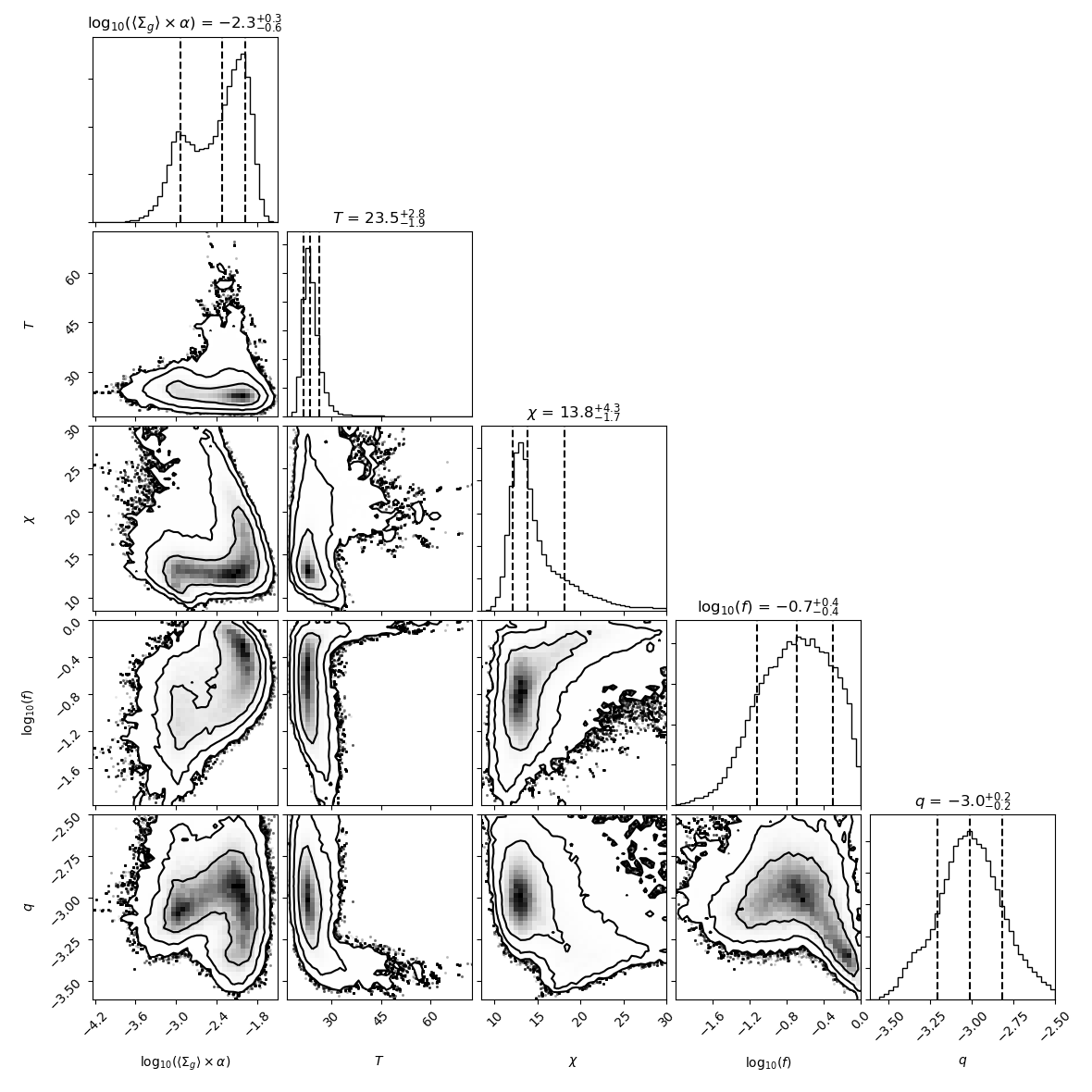
Figure 5: Optimization of the isothermal model with continuous grain sizes, with all 8 parameters. This corner plot shows the posterior probability distributions for 5 selected parameters, the other 3 being essentially unconstrained. The histograms plot the 1D probability density functions of the parameters indicated in titles along with their median values and 1$\sigma$ confidence intervals (i.e. at 16% and 84%), which are also shown by the vertical dashed lines. The contour plots show the marginalized 2D distributions (i.e. the 2D projection of the 8D posterior probability distribution), for the corresponding pairs of parameters. Contour levels are chosen at 0.68, 0.95 and 0.997.

Fig. 6 shows the predicted azimuthal intensity profiles corresponding to the maximum likelihood parameters: $\langle\Sigma_{g}\rangle=7.6$ g cm^-2, $\log_{10}(\alpha)=-2.7$, $a_{\rm max}=8.2$ cm, $\epsilon=10.4$, $T=22.7$ K, $\chi=14.9$, $f=0.25$, $q=-3.1$. Models without scattering, so with an albedo $\omega(\nu,\phi)=0$, yield similar results, i.e. the largest differences are found for $T=23.6$ K and $\chi=16.3$, and are all within the uncertainties. The model is, unsurprisingly, exactly coincident with the observations: widths, peak intensities, and the contrast at 342GHz are reproduced within 1%. The optical depth profiles reach optically thick values in the sub-mm, with a peak absorption optical depth of 2.9 at 342 GHz. Perhaps more suprising is the high absorption optical depth in cm-wavelengths, with a peak of 0.3, which, given the observed flux density, reflects the low temperatures and the small solid angle subtended by the elongated vortex. Such fairly high optical depths have also been predicted by Sierra et al. (2017).

Figure 6: Model azimuthal profiles predicted with a continuous grain population and the Lyra-Lin trapping prescriptions, and comparison with the Gaussian fits to the observed profiles, with flat baselines. Top: Intensity profiles. The maximum likelihood models at each each frequency are shown in thick solid lines. The optimization involves the comparison of a Gaussian fit to the model profiles (dashed) against the Gaussian fits to the observed profiles corrected for the effective angular resolutions (thin solid lines, see text for details). The almost perfect match reflects the reduced number of independent data points compared to the free parameters. Middle: Model optical depth profiles, normalized to the peak values indicated in the legend. Bottom: Corresponding grain albedos at each frequency.

The best fit parameters are all within the expected range, given the limits, except for the temperature $T=23.5^{+2.8}_{-1.9}$ K, which is significantly colder than the 35 K from the RT predictions in Boehler et al. (2018). This difference may be related to the dust population in the trap being heavily weighted to large grains compared to that originating the bulk of the sub-mm emission. Additional multi-frequency data are required to test this result for low temperatures, which could be due to the simplifications in this model, or in missing physical processes in the Lyra-Lin prescriptions (which are isothermal). An inadequate model would result in deviations from sufficiently detailed observations.

Another interesting result from the optimization of the isothermal model and steady-state model is the prediction of a very elongated vortex, $\chi=13.8^{+4.3}_{-1.7}$. This is in agreement with hydrodynamical simulations taylored to MWC 758, which resulted in $\chi=15\pm 2$. In a companion article (Baruteau et al. 2018), we reproduce the dust emission in Clumps 1 and 2 by means of dust+gas hydrodynamical simulations, using a 5$M_{\rm jup}$ body at 132 AU, which drives Clump 1, and a 1$M_{\rm jup}$ body at 33 AU, which drives Clump 2. The external companion is also required to account for the prominent spiral structure (as in Dong et al., 2015). Its mass is limited by recent $L^{\prime}$ high-contrast data to less than 10 M_jup assuming “hot start” conditions Reggiani et al. (2014). The internal companion is close to the thermal-IR point-source reported by Reggiani et al. (2014), whose $L^{\prime}$ magnitude is compatible with a 5 $M_{\mathrm{jup}}$ planet accreting at a rate of $10^{-6}M_{\mathrm{jup}}\mathrm{yr}^{-1}$.

3.3 The contrast between Clump 1 and Clump 2

In Figs. 1d and f, the peak intensity ratio $R$ between Clump 1 and Clump 2 at 342 GHz is $R_{342{\rm\,GHz}}=1.51\pm 0.01$. Yet, at 33 GHz, and at a similar angular resolution as the 342 GHz data, this ratio is $R_{33{\rm\,GHz}}>4.8$ at 3 $\sigma$, since the peak in Clump 1 is $29\pm 2.0$ $\mu$Jy beam^-1 in Fig. 1f.

From the smooted image $I^{c}_{33{\rm\,GHz}}$ shown in Fig. 2, we see that Clump 2 is indeed detected at 33 GHz, at the same location as at 342 GHz, and with a local peak intensity of $19\pm 5$ $\mu$Jy beam^-1, where the 1 $\sigma$ noise corresponds to the intensity of the spurious features in the field. Since the peak of $I^{c}_{33{\rm\,GHz}}$ without subtraction of Clump 1 is 51 $\mu$Jy beam^-1, we have an inter-clump contrast $R^{c}_{33{\rm\,GHz}}=2.7\pm 0.3$. In the natural-weights map $I^{c}_{342{\rm\,GHz}}$, this contrast is $R^{c}_{342{\rm\,GHz}}=1.55\pm 0.004$.

Some dust trapping may be at work also for Clump 2, since the 33 GHz signal in Fig. 2 appears somewhat more lopsided than at 342 GHz (the azimuthal contrast at the radius of Clump 2 is $\sim$1.5 in $I^{c}_{342{\rm\,GHz}}$ and $\sim$2.3 in $I^{c}_{33{\rm\,GHz}}$). However, the concentration of the cm-grains is not as effective as for Clump 1. We see that Clump 2 is likely more extended than Clump 1, explaining its non-detection in A-configuration angular resolutions. We note that even in the coarse maps, the inter-clump contrast is a factor $\sim$2 greater at 33 GHz than at 342 GHz, suggesting a deficit of cm-grains in Clump 2 when compared with Clump 1.

Since Clump 2 is found closer to the cavity edge than Clump 1, it is possible that the gas background is denser for Clump 2, such that the Stokes numbers are reduced. In the parametric model of Boehler et al. (2018), the mid-plane gas densities could be more than twice denser at 60 au compared to 80 au, with correspondingly lower Stokes number for Clump 2, which would result in less efficient trapping. Alternatively, the companion paper by Baruteau et al. (2018) models Clump 2 as a decaying vortex.

The continuum optical depths under Clump 2 are markedly lower than for Clump 1. Using the midplane temperature at a stellocentric radius of 50 au from Boehler et al. (2018), of 70 K, we obtain $\tau(33{\rm\,GHz})=0.006$ and $\tau(342{\rm\,GHz})=0.09$, with an index $\beta=1.17$. The non-detection of Clump 2 in A-configuration suggests that it is extended, so it is likely that this high $\beta$ index is intrinsic and not just due to the coarse beam. In the same coarse beam, the $\beta$ index for Clump 1 is 0.95, but Clump 1 is very compact and a meaningful $\beta$ index can only be obtained in the finest angular resolutions (for which $\beta=0.57$, see Sec. 3.1).

4 Conclusions

We presented new VLA observations at 33 GHz of MWC 758 that revealed disk emission concentrated in three regions, which present interesting differences with reprocessed 342 GHz ALMA data:

• Clump 1, originally detected by Marino et al. (2015), is an arc with a deprojected length of $0.24\arcsec\pm 0.006\arcsec$, FWHM. Clump 1 is $2.26\pm 0.04$ times more compact in azimuth at 33 GHz than at 342 GHz. Its radial width is $64$ mas$\pm$4 mas, and marginally resolved in our deconvolved model of the VLA A-configuration data, with an effective resolution of $\sim$48 mas. Correction for the finite angular resolution yields linear dimensions of $(37\pm 0.95\times 6.7\pm 0.64)\,\text{au}$, for a distance of 160 pc, and where the uncertainties do not account for systematics. The resulting aspect ratio is $\chi>5.3$ (at 3$\sigma$).

• Clump 2, which is the second local maximum at 342 GHz (Marino et al., 2015) in the outer disk, is also detected at 33 GHz, but is not as compact as Clump 1. Its intensity ratio relative to Clump 1 is $\sim$2 times less at 33 GHz.

The spectral trends in Clump 1 are quantitatively consistent with an isothermal model for dust trapping in an anticyclonic vortex using the Lyra-Lin prescription from Lyra & Lin (2013). The required physical conditions are all consistent with the body of information on MWC 758. This model makes a robust predictions for the vortex aspect ratio $\chi=13.8^{+4.3}_{-1.7}$ and temperature $T=23.5^{+2.8}_{-1.9}$ K. An elongated vortex is consistent with hydrodynamical simulations taylored to MWC 758 (Baruteau et al. 2018, submitted). This result suggests that the very long arc seen in the ALMA Band 4 observations reported by Cazzoletti et al. (2018) in HD 135344B also correspond to a very elongated vortex. The large optical depths required by such low temperatures and narrow aspect ratios, of order $\sim 1$ even in cm-wavelengths, have also been predicted in the generic models of Sierra et al. (2017), and could be tested with further multi-frequency observations of MWC 758. The model also constrains the gas surface densities $\Sigma_{g}$ and the turbulence parameter through $\log_{10}\left(\alpha\times\Sigma_{g}/\mathrm{g\,cm}^{-2}\right)\sim-2.3^{+0.3}_{-0.6}$. For a standard $\alpha\lesssim 10^{-3}$, $\Sigma_{g}$ is required to be larger by a factor of 3 to 10 compared to that inferred by Boehler et al. (2018) from the CO isotopologues.

The low signal from Clump 2 at 33 GHz may be due to a factor $\gtrsim 2$ larger gas density. This would result in less efficient aerodynamic coupling than in Clump 1. Alternatively Clump 2 may correspond to trapping in a decaying vortex, as suggested in Baruteau et al. (2018, submitted).

References

- Barge & Sommeria (1995) Barge P., Sommeria J., 1995, A&A, 295, L1
- Baruteau & Zhu (2016) Baruteau C., Zhu Z., 2016, MNRAS, 458, 3927
- Benisty et al. (2015) Benisty M., et al., 2015, A&A, 578, L6
- Biller et al. (2012) Biller B., et al., 2012, ApJ, 753, L38
- Birnstiel et al. (2013) Birnstiel T., Dullemond C. P., Pinilla P., 2013, A&A, 550, L8
- Boehler et al. (2017) Boehler Y., Weaver E., Isella A., Ricci L., Grady C., Carpenter J., Perez L., 2017, ApJ, 840, 60
- Boehler et al. (2018) Boehler Y., et al., 2018, ApJ, 853, 162
- Cárcamo et al. (2018) Cárcamo M., Román P. E., Casassus S., Moral V., Rannou F. R., 2018, Astronomy and Computing, 22, 16
- Carrasco-González et al. (2016) Carrasco-González C., et al., 2016, ApJ, 821, L16
- Casassus et al. (2013) Casassus S., et al., 2013, Nature, 493, 191
- Casassus et al. (2015) Casassus S., et al., 2015, ApJ, 812, 126
- Cazzoletti et al. (2018) Cazzoletti P., et al., 2018, preprint, (arXiv:1809.04160)
- Christiaens et al. (2018) Christiaens V., et al., 2018, A&A, 617, A37
- Cuzzi et al. (2008) Cuzzi J. N., Hogan R. C., Shariff K., 2008, ApJ, 687, 1432
- D’Alessio et al. (2001) D’Alessio P., Calvet N., Hartmann L., 2001, ApJ, 553, 321
- Dong et al. (2015) Dong R., Zhu Z., Rafikov R. R., Stone J. M., 2015, ApJ, 809, L5
- Dong et al. (2018) Dong R., et al., 2018, ApJ, 860, 124
- Foreman-Mackey et al. (2013) Foreman-Mackey D., Hogg D. W., Lang D., Goodman J., 2013, PASP, 125, 306
- Gaia Collaboration et al. (2016) Gaia Collaboration et al., 2016, A&A, 595, A1
- Goodman & Weare (2010) Goodman J., Weare J., 2010, Communications in Applied Mathematics and Computational Science, Vol.~5, No.~1, p.~65-80, 2010, 5, 65
- Grady et al. (2013) Grady C. A., et al., 2013, ApJ, 762, 48
- Isella et al. (2013) Isella A., Pérez L. M., Carpenter J. M., Ricci L., Andrews S., Rosenfeld K., 2013, ApJ, 775, 30
- Isella et al. (2014) Isella A., Chandler C. J., Carpenter J. M., Pérez L. M., Ricci L., 2014, ApJ, 788, 129
- Kataoka et al. (2014) Kataoka A., Okuzumi S., Tanaka H., Nomura H., 2014, A&A, 568, A42
- Koller et al. (2003) Koller J., Li H., Lin D. N. C., 2003, ApJ, 596, L91
- Lyra & Klahr (2011) Lyra W., Klahr H., 2011, A&A, 527, A138
- Lyra & Lin (2013) Lyra W., Lin M.-K., 2013, ApJ, 775, 17
- Lyra et al. (2009) Lyra W., Johansen A., Zsom A., Klahr H., Piskunov N., 2009, A&A, 497, 869
- Macías et al. (2017) Macías E., Anglada G., Osorio M., Torrelles J. M., Carrasco-González C., Gómez J. F., Rodríguez L. F., Sierra A., 2017, ApJ, 838, 97
- Marino et al. (2015) Marino S., Casassus S., Perez S., Lyra W., Roman P. E., Avenhaus H., Wright C. M., Maddison S. T., 2015, ApJ, 813, 76
- Mittal & Chiang (2015) Mittal T., Chiang E., 2015, ApJ, 798, L25
- Miyake & Nakagawa (1993) Miyake K., Nakagawa Y., 1993, Icarus, 106, 20
- Muto et al. (2015) Muto T., et al., 2015, PASJ, 67, 122
- Pérez et al. (2014) Pérez L. M., Isella A., Carpenter J. M., Chandler C. J., 2014, ApJ, 783, L13
- Ragusa et al. (2017) Ragusa E., Dipierro G., Lodato G., Laibe G., Price D. J., 2017, MNRAS, 464, 1449
- Rau & Cornwell (2011) Rau U., Cornwell T. J., 2011, A&A, 532, A71
- Regály et al. (2012) Regály Z., Juhász A., Sándor Z., Dullemond C. P., 2012, MNRAS, 419, 1701
- Reggiani et al. (2014) Reggiani M., et al., 2014, ApJ, 792, L23
- Sándor et al. (2011) Sándor Z., Lyra W., Dullemond C. P., 2011, ApJ, 728, L9
- Shakura & Sunyaev (1973) Shakura N. I., Sunyaev R. A., 1973, A&A, 24, 337
- Sierra et al. (2017) Sierra A., Lizano S., Barge P., 2017, ApJ, 850, 115
- Varnière & Tagger (2006) Varnière P., Tagger M., 2006, A&A, 446, L13
- Weidenschilling (1977) Weidenschilling S. J., 1977, MNRAS, 180, 57
- Wright & Barlow (1975) Wright A. E., Barlow M. J., 1975, MNRAS, 170, 41
- Zhu & Baruteau (2016) Zhu Z., Baruteau C., 2016, MNRAS, 458, 3918
- Zhu & Stone (2014) Zhu Z., Stone J. M., 2014, ApJ, 795, 53
- de Val-Borro et al. (2007) de Val-Borro M., Artymowicz P., D’Angelo G., Peplinski A., 2007, A&A, 471, 1043
- van der Marel et al. (2013) van der Marel N., et al., 2013, Science, 340, 1199
- van der Marel et al. (2015a) van der Marel N., van Dishoeck E. F., Bruderer S., Pérez L., Isella A., 2015a, A&A, 579, A106
- van der Marel et al. (2015b) van der Marel N., Pinilla P., Tobin J., van Kempen T., Andrews S., Ricci L., Birnstiel T., 2015b, ApJ, 810, L7
- van der Marel et al. (2016a) van der Marel N., van Dishoeck E. F., Bruderer S., Andrews S. M., Pontoppidan K. M., Herczeg G. J., van Kempen T., Miotello A., 2016a, A&A, 585, A58
- van der Marel et al. (2016b) van der Marel N., Cazzoletti P., Pinilla P., Garufi A., 2016b, ApJ, 832, 178
- van der Plas et al. (2017) van der Plas G., Ménard F., Canovas H., Avenhaus H., Casassus S., Pinte C., Caceres C., Cieza L., 2017, A&A, 607, A55