Orbital Angular Momentum Induced by Nonabsorbing Optical Elements through Space-variant Polarization-state Manipulations

Abstract

To manipulate orbital angular momentum (OAM) carried by light beams, there is a great interest in designing various optical elements from the deep-ultraviolet to the microwave. Normally, the OAM variation introduced by optical elements can be attributed to two terms, namely the dynamic and geometric phases. Up till now, the dynamic contribution induced by optical elements has been clearly recognized. However, the contribution of geometric phase still seems obscure, especially considering the vector vortex beams. In this work, an analytical formula is derived to fully describe the OAM variation introduced by the nonabsorbing optical elements, which perform space-variant polarization-state manipulations. It is found that the geometric contribution can be further divided into two parts: one is directly related to optical elements and the other one explicitly relies solely on the vortices before and after the transformations. Based on this result, the same OAM variation can be achieved with different combinations of the dynamic and/or geometric contributions. With numerical simulations, it is shown that transformation of the optical vortices can be fully and flexibly designed with a family of optical elements. We believe that these results are helpful to understand the effect of optical elements and offer a new perspective to design the optical elements for manipulating the OAM carried by light beams.

I Introduction

Light can carry both spin and orbital angular momentum (SAM and OAM), which are corresponding to the polarization and spatial degrees of freedom, respectively Padgett et al. (2004); Franke-Arnold et al. (2008); Barnett (2002). Under the paraxial approximation, the SAM and OAM are separable within isotropic homogeneous media Yao and Padgett (2011). The SAM per photon has a value of $\pm\hbar$ (the reduced Planck’s constant) corresponding to left-/right-handed circular polarization, while the OAM would be more intriguing even under paraxial approximation. For a scalar vortex beam, the OAM would be $l\hbar$ per photon for the optical field with a spiral wavefront of $\exp(il\phi)$, where $l$ can be any integer Allen et al. (1992). However, for vector vortex beams, it would be more complicated since the space-variant state of polarization (SOP) would attribute to the OAM charge Wang et al. (2010); Niv et al. (2006). To address it, several approaches have been proposed to extract the geometric contribution through the high-order Poincaré spheres Milione et al. (2011, 2012) or introducing the topological Pancharatnam charge Zhang et al. (2015). However, when the light beam is transformed, there are no explicit formulas to describe the corresponding variation of OAM charge due to the geometric contribution. Such an explicit formula would be significant while analyzing the OAM evolution in an optical system and tailoring the OAM carried by vortex beams, since the spin-orbit interactions (SOIs) are inevitable.

The SOI is a general basic phenomenon in manipulations of light beams and photons, which has been observed in light propagating Bliokh et al. (2008, 2017), scattering O’Connor et al. (2014), focusing Zhao et al. (2007), etc. The SOIs have evoked some interesting investigations of physical phenomena such as the spin-Hall effect Onoda et al. (2004); Hosten and Kwiat (2008); Bliokh et al. (2015), extraordinary momentum states Bliokh et al. (2014) and even extended to cavity-quantum electrodynamics (CQEDs) Deng et al. (2014). In the new reality of nano-optics, SOI is essential in both the physical conception and device design and should be also taken into account for nano-optical systems. Recently, several nano-optics platforms have been employed to replicate the functionality of common optical elements such as polarizers, wave retarders, etc., which have shown promising abilities to manipulate both polarization and phase distributions of optical beams Arbabi et al. (2015). In particular, SOI has emerged as a powerful mean to tailor the OAM carried by scalar vortex beams, which can be achieved by optical elements to perform space-variant polarization-state manipulations (e.g. spiral phase plates Yu et al. (2011), q-plates Marrucci et al. (2006); Bomzon et al. (2002), J-plates Devlin et al. (2017)). In these transformations, the desired spiral wavefronts of light beams are introduced by steering dynamic phase and/or geometric phase. However, the SOIs would be much more complicated while considering vector vortex beams passing through optical elements, where the geometric phase has to be seriously considered to evaluate the OAM of light beams Souza et al. (2007); Ma et al. (2016). Furthermore, more interesting phenomena and flexible manipulations of optical vortices can be achieved with SOIs in inhomogeneous or anisotropic media. The manipulation of SOIs can release the full potential of information processing through an effective utilization of both SAM and OAM. Thus the generation, measurement, and control of optical vortices via SOIs have attracted a considerable amount of attentions recently. Definitely, two cruxes, namely OAM variation and geometric phase, are inevitable in the SOIs of optical vortices. Thus, there are two questions that should be addressed. First, whether the OAM variation introduced by optical element is distinguishable in terms of dynamic and geometric phases for arbitrary vortex beams? And second, whether there are various designs of optical elements to tailor OAM as steering SAM? These issues are quite appealing for both the theoretical understanding and practical application.

In this work, we have tackled both issues. An explicit formula is deduced to describe the OAM variation introduced by the nonabsorbing optical elements, which perform space-variant polarization-state manipulations. It is found that the geometric contribution can be further divided into two parts: one is directly related to optical elements and the other one explicitly relies solely on the optical vortices before and after the transformations. Specifically, an intuitive picture is presented to obtain deeper insight into how the dynamic and geometric phases are involved. As a concrete example, we present the design rule for transformations from one scalar vortex to another to show the flexibility for the same OAM variation. Furthermore, the designs of transforming vector vortex are also shown. At the end, the features of previously reported optical elements would be discussed under our theoretical framework.

II Theoretical principle

II.1 OAM of an optical vortex beam

Under the paraxial approximation, an electric field of a fully polarized vector vortex beam propagating along $\mathbf{z}$ direction with the angular frequency $\omega$ can be written as Torres and Torner (2011)

$$\mathbf{E}\left(x,y\right)=i\omega\left(\alpha\mathbf{\hat{x}}+\beta\mathbf{\hat{y}}+\frac{i}{k}\left(\frac{\partial\alpha}{\partial x}+\frac{\partial\beta}{\partial y}\right)\mathbf{\hat{z}}\right)e^{ikz},$$ (1)

where $\alpha(\beta)$ represents the complex amplitude of $x(y)-$component of electric field, as a function of $(x,y)$ (omitted for simplicity). Then the SOP of such a beam can be described by a $2\times 1$ Jones vector $\left|a\right\rangle=(a_{x},a_{y})^{\mathrm{T}}$, where $a_{x}(a_{y})=\alpha(\beta)/\sqrt{I_{\text{E}}}$ represents the normalized complex amplitude and $I_{\text{E}}=|\alpha|^{2}+|\beta|^{2}$ is the electric intensity of light. The corresponding Stokes vector $\mathbf{S=}$$(S_{1},S_{2},S_{3})^{\mathrm{T}}$ is defined by $S_{j}=\left\langle a|\bm{\sigma}_{j}|a\right\rangle(j=1,2,3)$, where $\bm{\sigma}_{j}$ are the Pauli matrices and $S_{0}=\left\langle a|\bm{\sigma}_{0}|a\right\rangle$, where $\bm{\sigma}_{0}$ equals $2\times 2$ identity matrix Gutiérrez-Vega (2011). Thus, $S_{0}=1$ presents fully polarized light and $S_{3}=\pm 1$ presents left/right circularly polarized field $\left|\mathrm{e}_{\pm}\right\rangle=(1/\sqrt{2})(1,\pm i)^{\mathrm{T}}$. By mapping $\mathbf{S}$ directly in three-dimensional Cartesian coordinates, the Poincaré sphere can be constructed and the corresponding azimuth ($\psi_{\mathrm{S}}$) and ellipticity ($\chi_{\mathrm{S}}$) angles of SOP can be resolved by $\tan(2\psi_{\mathrm{S}})=S_{2}/S_{1}$ and $\sin(2\chi_{\mathrm{S}})=S_{3}/S_{0}$ Born and Wolf (2013).

With the aforementioned notations, the average OAM charge for a fully polarized paraxial vector vortex beam can be calculated by OAM density $\mathbf{j}_{z}^{\mathrm{o}}$ as Allen and Padgett (2000); Barnett (2002)

$$\bar{l} =\frac{\iint\mathbf{j}_{z}^{\text{o}}rdrd\phi}{\omega\epsilon_{0}\iint I_{\text{E}}S_{0}rdrd\phi}.$$ (2)

It should be noticed that the average OAM charge depends on not only the distribution of SOP but also the intensity distribution ($I_{\text{E}}$) of beams. Thus, equation (2) is also applicable to characterize the non-vortex (‘asymmetry’) OAM of beams without the wavefront singularities Bekshaev et al. (2003). Next, similar to our previous work Zhang et al. (2015), the OAM density can be expressed by introducing the Pancharatnam connection between two different SOPs Berry (1987). Here, circularly polarized fields are adopted as reference. Then, the phase difference for any field $\left|a\right\rangle=(a_{x},a_{y})^{\mathrm{T}}$ can be written as $\psi_{\mathrm{P\pm}}=\arg\left(\left\langle\mathrm{e}_{\pm}|a\right\rangle\right).$ According to Ref. Zhang et al. (2015), the OAM density can be obtained by

$$\frac{\mathbf{j}_{z}^{\text{o}}}{\omega\epsilon_{0}I_{\text{E}}}=\frac{1}{2}\left((1+S_{3})\frac{\partial\psi_{\mathrm{P+}}}{\partial\phi}+(1-S_{3})\frac{\partial\psi_{\mathrm{P-}}}{\partial\phi}\right).$$ (3)

The detailed deduction of equations (2) and (3) can be found in Appendix A.

In equation (3), the derivative of $\psi_{\mathrm{P\pm}}$ is known as the topological Pancharatnam charge Niv et al. (2006); Zhang et al. (2015). With equations (2) and (3), the average OAM charge carried by the light beam can be fully expressed with the SAM ($S_{3}$) and the topological Pancharatnam charge ($\partial\psi_{\mathrm{P\pm}}/\partial\phi$), which can depict the OAM states on a single Poincaré sphere as Refs. Zhang et al. (2015); Zhao et al. (2017). Thus, the corresponding geometric phase for any transformations can be conveniently identified on the same Poincaré spheres. Such a representation can succinctly and elegantly describe the OAM of a light beam, where the contribution from the space-variant SOP of vector vortex has been naturally embedded. Moreover, the OAM charge can be identified with standard measurement of Stokes parameters and interferometry. As shown in the following part, our approach could be conveniently employed to design optical elements for manipulating the OAM charge and investigate the OAM evolution of light beam propagating in an optical system.

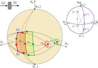
Figure 1: Manipulating both SAM and OAM. For the same transformation from $|a\rangle$ to $|b\rangle$, different linear operations (i.e., with different Jones matrices $\mathbf{J}_{i}$, where $i=1,2$) can induce distinct OAM charge since there are different combinations of dynamic phases $\psi_{\mathrm{D}_{i}}$ and geometric phases $\Omega_{\mathrm{G}_{i}}/4$ ($i=1,2$). The magnitude of $\Omega_{\mathrm{G}_{i}}$ depends on the eigen-polarization $|q_{1_{i}}\rangle$ and birefringent phase difference $\psi_{\mathrm{B}_{i}}$ of $\mathbf{J}_{i}$. The inset shows that one linear operation can transform a pair of orthogonal SOP scalar vortices $|a^{\pm}\rangle$ into another pair of SOP scalar vortices $|b^{\pm}\rangle$ with different OAM variations at the same time.

II.2 OAM variation induced by non-absorbing optical elements

Here, we consider a scenario that a light passes through a nonabsorbing optical element. The SOPs of input and output fields are denoted as $\left|a\right\rangle=(a_{x},a_{y})^{\mathrm{T}}$ and $\left|b\right\rangle=(b_{x},b_{y})^{\mathrm{T}}$, respectively. And the optical element is characterized by a unitary Jones matrix $\mathbf{J}$, i.e., $\mathbf{J}^{\dagger}=\mathbf{J}^{-1}$. Thus, the light field transformation can be described as $|b\rangle=\mathbf{J}|a\rangle$ (see Fig. 1). Mathematically, the eigenvalues and eigenstates of $\mathbf{J}$ are $\mu_{1(2)}$ and $|q_{1(2)}\rangle$, respectively. Then the corresponding Stokes vectors for eigenstates can be calculated as $\mathbf{S}^{\mathrm{J}}=\mathbf{S}^{q_{1}}=-\mathbf{S}^{q_{2}}=(S_{1}^{\mathrm{J}},S_{2}^{\mathrm{J}},S_{3}^{\mathrm{J}})^{\mathrm{T}}$, where $S_{j}^{\mathrm{J}}=\left\langle q_{1}|\bm{\sigma}_{j}|q_{1}\right\rangle$. With these notations, the variation of OAM density can be deduced according to equation (3). For transforming state $\left|a\right\rangle$ to state $\left|b\right\rangle$, beyond SAM variation from $S_{3}^{a}$ to $S_{3}^{b}$, there is also a variation from $\psi_{\mathrm{P\pm}}^{a}$ to $\psi_{\mathrm{P\pm}}^{b}$, where the superscript $a(b)$ refers to the parameters related to state $|a\rangle$($|b\rangle$). According to Refs. Gutiérrez-Vega (2011); Martínez-Fuentes et al. (2012), the phase difference $\psi_{\mathrm{P\pm}}^{a\rightarrow b}=\psi_{\mathrm{P\pm}}^{b}-\psi_{\mathrm{P\pm}}^{a}$ can be rewritten as

$$\psi_{\mathrm{P\pm}}^{a\rightarrow b}=\psi_{\mathrm{D}}-\frac{\Omega_{ab\mathrm{e}_{\pm}}^{\mathrm{C}}}{2}+\frac{\Omega_{abb^{\dagger}a^{\dagger}}^{\mathrm{J}}}{4},$$ (4)

where $\psi_{\mathrm{D}}=\mathrm{arg}(\mu_{1}\mu_{2})/2$ presents the dynamic phase as the light beam propagating through the optical element and $\Omega_{ab\mathrm{e}_{\pm}}^{\mathrm{C}}\big{/}2$ is the geometric phase introduced by varied SOP between the output and input fields, which corresponds to parallel transport of the state around a closed loop ($|a\rangle\rightarrow|b\rangle\rightarrow|\mathrm{e}_{\pm}\rangle\rightarrow|a\rangle$) on the Poincaré sphere (see Fig. 2(a)). While $\Omega_{abb^{\dagger}a^{\dagger}}^{\mathrm{J}}$ is a spherical quadrangle corresponding to the closed trajectory $|a\rangle\rightarrow|b\rangle\rightarrow|b_{\mathrm{J}}^{\dagger}\rangle\rightarrow|a_{\mathrm{J}}^{\dagger}\rangle\rightarrow|a\rangle$, as blue area shown in Fig. 2(b) (also see Fig. 6), where $|a_{\mathrm{J}}^{\dagger}\rangle(|b_{\mathrm{J}}^{\dagger}\rangle)$ holds the Stokes vector $\mathbf{S}^{a_{\mathrm{J}}^{\dagger}(b_{\mathrm{J}}^{\dagger})}=\mathbf{S}^{a(b)}-2(\mathbf{S}^{a(b)}\cdot\mathbf{S}^{\mathrm{J}})\mathbf{S}^{\mathrm{J}}$. It can be found that the term $\Omega_{abb^{\dagger}a^{\dagger}}^{\mathrm{J}}\big{/}4$ is the geometric phase explicitly related with the optical element $\mathbf{J}$. It should be noticed that although both $\Omega_{ab\mathrm{e}_{\pm}}^{\mathrm{C}}\big{/}2$ and $\Omega_{abb^{\dagger}a^{\dagger}}^{\mathrm{J}}\big{/}4$ are related to the geometric phases, they would affect the final OAM density with different manners. To clearly describe the contribution of optical element and the impact of varied SOP between input and output fields, the variation of OAM density can be deduced with equation (4) as follows:

$$\frac{\Delta\mathbf{j}_{z}^{\text{o}}}{\omega\epsilon_{0}I_{\text{E}}}= \frac{\partial\psi_{\mathrm{D}}}{\partial\phi}+\frac{\partial}{\partial\phi}\left(\frac{\Omega_{abb^{\dagger}a^{\dagger}}^{\mathrm{J}}}{4}\right)$$

$$+\left[S_{3}^{a}\frac{\partial\psi_{\mathrm{S}}^{a}}{\partial\phi}-S_{3}^{b}\frac{\partial\psi_{\mathrm{S}}^{b}}{\partial\phi}-\frac{\partial}{\partial\phi}\left(\frac{\Omega_{abb^{\dagger}a^{\dagger}}^{\mathrm{C}}}{4}\right)\right],$$ (5)

where $\Omega_{abb^{\dagger}a^{\dagger}}^{\mathrm{C}}$ is a spherical quadrangle defined by states $|a\rangle$, $|b\rangle$, $|b_{\mathrm{C}}^{\dagger}\rangle$ and $|a_{\mathrm{C}}^{\dagger}\rangle$ as green area shown in Fig. 2(b), where $|a_{\mathrm{C}}^{\dagger}\rangle(|b_{\mathrm{C}}^{\dagger}\rangle)$ holds the Stokes vector $\mathbf{S}^{a_{\mathrm{C}}^{\dagger}(b_{\mathrm{C}}^{\dagger})}=\mathbf{S}^{a(b)}-2(\mathbf{S}^{a(b)}\cdot\mathbf{S}^{\mathrm{e}_{+}})\mathbf{S}^{\mathrm{e}_{+}}$. It is easy to find $\Omega_{abb^{\dagger}a^{\dagger}}^{\mathrm{C}}=\Omega_{ab\mathrm{e}_{+}}^{\mathrm{C}}+\Omega_{ab\mathrm{e}_{-}}^{\mathrm{C}}$ (see Appendix B for details). According to equation (5), the OAM variation can be attributed to three terms. The first term ($C_{\mathrm{d}}=\frac{\partial\psi_{\mathrm{D}}}{\partial\phi}$) is dynamic contribution and presents the OAM variation induced by the dynamic phase delay, which only depends on $\psi_{\mathrm{D}}$ of the optical element ($\mathbf{J})$, regardless of the SOP of input beam. The rest two terms present the geometric contributions ($C_{\mathrm{g}}$) that rely on the optical elements as well as the SOP of light beams. Specifically, the second term ($C_{\mathrm{g}}^{\mathrm{J}}=\frac{1}{4}\frac{\partial}{\partial\phi}\left(\Omega_{abb^{\dagger}a^{\dagger}}^{\mathrm{J}}\right)$) is related to eigen-polarization $\mathbf{\mathbf{S}^{\mathrm{J}}}$ (i.e. $|q_{1}\rangle$) and birefringent phase difference $\psi_{\mathrm{B}}$ (equals $\mathrm{arg}(\mu_{1}^{\ast}\mu_{2})$) of the adopted transformation matrix $\mathbf{J}$ (see corresponding spherical quadrangle $\Omega_{\mathrm{G}_{i}}$ in Fig. 1 or $\Omega_{abb^{\dagger}a^{\dagger}}^{\mathrm{J}}$ in Fig. 2(b)). The third (rest) term ($C_{\mathrm{g}}^{\mathrm{V}}$) explicitly depends on the input and output fields themselves and presents the geometric contribution stemming from the different SOP distributions of input and output vortices. Namely $C_{\mathrm{g}}^{\mathrm{V}}$ can be fully determined by $\mathbf{S}^{a}$ and $\mathbf{S}^{b}$ (for $\Omega_{abb^{\dagger}a^{\dagger}}^{\mathrm{C}}$, see Fig. 2(b)). Thus, the geometric contribution of $C_{\mathrm{g}}^{\mathrm{V}}$ would be determined once the input and target output vortex beams are given. However, there are still various combinations of dynamic ($C_{\mathrm{d}}$) and geometric ($C_{\mathrm{g}}^{\mathrm{J}}$) contributions to achieve the same OAM variation. Thus, equation (5) indicates that it would be greatly flexible to design the optical element for vortex beam transformations. It should be mentioned that this has not been fully perceived and explored at present. To demonstrate the mentioned above, some simulations have been carried out for both the scalar and vector vortex beams.

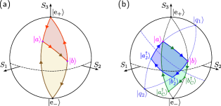
Figure 2: Solid angle associated with geometric phase in the transformation. (a) Geodesic triangle $\Omega_{ab\mathrm{e}_{+}}^{\mathrm{C}}$ (reddish) and $\Omega_{ab\mathrm{e}_{-}}^{\mathrm{C}}$ (buff) on the Poincaré sphere. (b) Spherical quadrangle $\Omega_{abb^{\dagger}a^{\dagger}}^{\mathrm{J}}$ (blue) on the Poincaré sphere, which is a portion of lune of dihedral angle defined by states $|a\rangle$, $|b\rangle$ and $|q_{1(2)}\rangle$. The state $|a_{\mathrm{J}}^{\dagger}\rangle(|b_{\mathrm{J}}^{\dagger}\rangle)$ is a reflection of state $|a\rangle(|b\rangle)$ referring to mirror plane of a great circle, which is perpendicular to the axis joining the states $|q_{1}\rangle$ and $|q_{2}\rangle$. Similarly, spherical quadrangle $\Omega_{abb^{\dagger}a^{\dagger}}^{\mathrm{C}}$ (green) is a portion of lune of dihedral angle defined by states $|a\rangle$, $|b\rangle$ and $|\mathrm{e}_{\pm}\rangle$. The state $|a_{\mathrm{C}}^{\dagger}\rangle(|b_{\mathrm{C}}^{\dagger}\rangle)$ is a reflection of state $|a\rangle(|b\rangle)$ referring to mirror plane of the equator.

III Transformations on scalar vortices

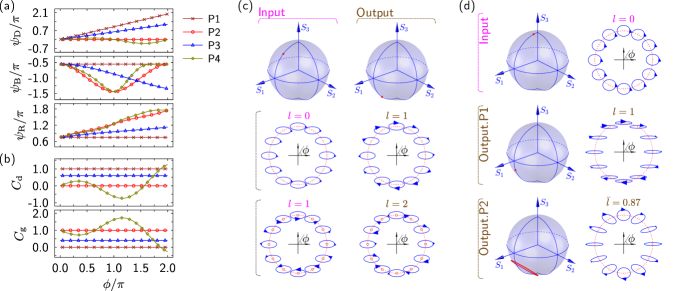
Figure 3: Transformations on scalar vortices. (a) The design parameters $\{\psi_{\mathrm{D}},\psi_{\mathrm{B}},\psi_{\mathrm{R}}\}$ of Jones matrices for optical plates P1–P4 from the top down. (b) The contributions for OAM variations from dynamic term $C_{\mathrm{d}}$ and geometric term $C_{\mathrm{g}}$ for designed input SOP $\{2\psi_{\mathrm{S}},2\chi_{\mathrm{S}}\}=\{0,50^{\circ}\}$. Note that we set $I_{\mathrm{E}}(\phi)=1$. (c) SOP trace on the Poincaré sphere (top panel) and spatial distribution of SOP (middle and bottom panels) for input (left panel) and output (right panel) fields with a designed P2P transformation. For the same input SOP but different OAM charges ($l=0$ (middle panel) or $l=1$ (bottom panel)), they can be transferred to both the same SOP and OAM variation by any of P1–P4. (d) SOP trace on the Poincaré sphere (left panel) and spatial distribution of SOP (left panel) for input fields with SOP $\{2\psi_{\mathrm{S}},2\chi_{\mathrm{S}}\}=\{0,80^{\circ}\}$ (top panel). The transferred fields are not the same due to different attributes of dynamic (P1, middle panel) and geometric (P2, bottom panel) contributions.

First, the point-to-point (P2P) transformation is demonstrated on the Poincaré sphere for a scalar vortex beam with the same OAM variation but different designs, as sketched in Fig. 1. According to equation (5), it can be found that $C_{\mathrm{g}}^{\mathrm{V}}=0$ for P2P transformation of scalar vortex. Thus there are two contributions for the OAM variation. The first one is the dynamic contribution ($C_{\mathrm{d}}$), which is determined by $\psi_{\mathrm{D}}$ of optical elements. The second term is geometric contribution ($C_{\mathrm{g}}^{\mathrm{J}}$), which stems from geometric phase $\Omega_{\mathrm{G}}/4$ depending on the $|q_{1}\rangle$ and $\psi_{\mathrm{B}}$. As a scalar vortex, the input light beam can be fully described by SOP of $\{2\psi_{\mathrm{S}},2\chi_{\mathrm{S}}\}$ and OAM charge of $l$. It should be noted that the SOPs of the scalar vortices are space-invariant, so $\{2\psi_{\mathrm{S}},2\chi_{\mathrm{S}}\}$ are $(x,y)$-independent. For the sake of simplicity but without loss of generality, $\psi_{\mathrm{S}}=0$ is settled since the absolute azimuth angle is irrelevant due to the rotation symmetry of the coordinate. Thus, the input scalar vortex can be expressed as $|a^{+}\rangle=e^{il\phi}(\cos(\chi_{\mathrm{S}}),i\sin(\chi_{\mathrm{S}}))^{\mathrm{T}}$. The output vortex ($|b^{+}\rangle$) is considered as $|b^{+}\rangle=e^{i(l+\Delta l)\phi}(\cos(\chi_{\mathrm{S}}),-i\sin(\chi_{\mathrm{S}}))^{\mathrm{T}}$ with a flipped handedness and OAM variation of $\Delta l$ after a optical element, which is described by Jones matrix $\mathbf{J}$ (see the inset of Fig. 1). It is easy to find that, for such a transformation $|b^{+}\rangle=\mathbf{J}|a^{+}\rangle$, the term $e^{il\phi}$ can be canceled so that the transformation is independent on OAM charge of input beam. Generally, $\mathbf{J}$ would be linearly birefringent without considering chiral or magneto-optic materials, thus the eigenstates of $\mathbf{J}$ are two linear and orthogonal eigen-polarizations. Considering the unitary nature of $\mathbf{J}$, the eigenvalues of $\mathbf{J}$ are given by $e^{i\psi_{\mathrm{D}}}\{e^{-i\psi_{\mathrm{B}}/2},e^{i\psi_{\mathrm{B}}/2}\}$ with dynamic phase delay $\psi_{\mathrm{D}}$ and birefringent phase difference $\psi_{\mathrm{B}}$. And the orthogonal eigen-polarizations can be written as $\mathbf{R}(\psi_{\mathrm{R}})(1,0)^{\mathrm{\mathrm{T}}}$ and $\mathbf{R}(\psi_{\mathrm{R}})(0,1)^{\mathrm{T}}$, where $\mathbf{R(\cdot)}$ is the standard rotation matrix and $\psi_{\mathrm{R}}$ is the orientation angle of linear eigen-polarizations. Thus, for the considered optical elements, the transformation matrix $\mathbf{J}$ can be determined by three parameters $\{\psi_{\mathrm{D}}(\phi),\psi_{\mathrm{B}}(\phi),\psi_{\mathrm{R}}(\phi)\}$ with each $\phi$

$$\mathbf{J}=e^{i\psi_{\mathrm{D}}}\left(\begin{array}[]{cc}\cos\left(\frac{\psi_{\mathrm{B}}}{2}\right)-i\sin\left(\frac{\psi_{\mathrm{B}}}{2}\right)\cos\left(2\psi_{\mathrm{R}}\right)&-i\sin\left(\frac{\psi_{\mathrm{B}}}{2}\right)\sin\left(2\psi_{\mathrm{R}}\right)\\ -i\sin\left(\frac{\psi_{\mathrm{B}}}{2}\right)\sin\left(2\psi_{\mathrm{R}}\right)&\cos\left(\frac{\psi_{\mathrm{B}}}{2}\right)+i\sin\left(\frac{\psi_{\mathrm{B}}}{2}\right)\cos\left(2\psi_{\mathrm{R}}\right)\end{array}\right).$$ (6)

It should be noticed that there are only two equations ($|b^{+}\rangle=\mathbf{J}|a^{+}\rangle$) to confine the relations of such three parameters. Thus, there would be various strategies to set the $\mathbf{J}$ with the same transformation result. In other words, once the dynamic phase delay $\psi_{\mathrm{D}}(\phi)$ is assigned, a combination of $\{\psi_{\mathrm{B}}(\phi),\psi_{\mathrm{R}}(\phi)\}$ can always be found. Obviously, it is a family of optical plates to perform the P2P transformation that only relies on input SOP, regardless of the carried OAM charge (details are discussed in Appendix C). To demonstrate such unique feature, some simulations have been carried out.

In Fig. 3, four different optical plates (denoted as P1–P4) are designed to transform left-handed elliptical polarization ($\{2\psi_{\mathrm{S}},2\chi_{\mathrm{S}}\}=\{0,50^{\circ}\}$) vortex to right-handed elliptical polarization ($\{2\psi_{\mathrm{S}},2\chi_{\mathrm{S}}\}=\{0,-50^{\circ}\}$) vortex with $\Delta l=1$. Figure 3(a) shows the parameters of $\mathbf{J}$ for each optical plate and Fig. 3(b) shows the corresponding dynamic term $C_{\mathrm{d}}$ and geometric term $C_{\mathrm{g}}^{\mathrm{J}}$ that would induce the OAM variations (it should be noted that $C_{\mathrm{g}}^{\mathrm{V}}=0$). For P1 and P2, the OAM variation is purely induced by dynamic or geometric contributions, respectively. Both $\psi_{\mathrm{B}}$ and $\psi_{\mathrm{R}}$ keep constant for P1 while $\psi_{\mathrm{D}}$ keeps constant for P2. As a comparison, both dynamic and geometric terms would contribute to the OAM variation for P3 and P4. Both $C_{\mathrm{d}}$ and $C_{\mathrm{g}}$ are designed as homogeneous and inhomogeneous distribution along $\phi$ for P3 and P4, respectively. Obviously, P4 is a more general and flexible example. Moreover, the corresponding SOP on the Poincaré sphere and the electric field distribution have been calculated for each optical plate to verify the equivalence of the considered transformations. As expected, the final results are the same for P1–P4 as shown in Fig. 3(c). It can also be found that the same OAM variation ($\Delta l=1$) can be obtained with input of $l=0$ or $l=1$ for P1–P4. It coincides with that the OAM variation is independent of the input OAM charge.

It should be mentioned that if the SOP of input light changes, P1–P4 will introduce different transformations since the geometric contribution depends on the SOP of the input beam. Thus, different designs of optical plates would introduce diverse variations of SAM and OAM when the SOP of input beam does not match the designed one. Figure 3(d) shows the transformations for input plane-wave with polarization $\{2\psi_{\mathrm{S}},2\chi_{\mathrm{S}}\}=\{0,80^{\circ}\}$ by P1 and P2. For P1, the output is still a scalar vortex with $l=1$ since there is the only pure dynamic contribution as shown in Fig. 3(d). However, the average OAM variation $\Delta\bar{l}$ would equal 0.87 for P2 and the output would be a vector vortex as shown in Fig. 3(d). The reason is that both two geometrical terms would contribute to the OAM variation (see Fig. 7). For the orthogonal input SOPs (antipodal points on the Poincaré sphere), there are equal but opposite geometric contributions since they have opposite evolution direction on the Poincaré sphere. Thus, the same dynamic term $C_{\mathrm{d}}$ and opposite geometric term $C_{\mathrm{g}}$ would be introduced and the final result is $\Delta\bar{l}\propto C_{\mathrm{d}}\pm C_{\mathrm{g}}$. For a desired OAM variation with the given SOP, the introduced contributions can be dynamic and/or geometric. Thus, the design of P2P transformations is flexible and fully controllable according to requirements. But it should be noticed that the dynamic phase based optical elements have a SOP-independent response while geometric phase based optical elements are completely SOP-dependent. Thus, the SOP-bandwidth of the optical elements would be narrower if more geometric contribution is introduced. Such issue should be considered for specific applications.

IV Transformations on vector vortices

More generally, equation (5) can be applied on transforming vector vortices. As shown in Fig. 4(a), the input beam is a cylindrical vortex with $2\chi_{\mathrm{S}}=30^{\circ}$ and $\bar{l}=0$ while the output beam is another cylindrical vortex with $2\chi_{\mathrm{S}}=-30^{\circ}$ and $\bar{l}=1$ (see Appendix D and Fig. 8 for $\{2\psi_{\mathrm{S}},2\chi_{\mathrm{S}}\}$ of the input and output beams). For such a transformation, the linearly birefringent unitary $\mathbf{J}$ is employed. By numerically solving the $\mathbf{J}$, the design parameters for three different optical plates (named P5–P7) are displayed in Fig. 4(b). The corresponding dynamic and geometric contributions are given in Fig. 4(c). It can be found that the values of $C_{\mathrm{g}}^{\mathrm{V}}$ are the same but not equal to zero. For these cases, the optical elements have to be meticulously designed to achieve average OAM variation of $\Delta\bar{l}=1$. Similar to P2P transformations, P5 is designed with only dynamic contribution $C_{\mathrm{d}}$ and P6 is with only geometric contribution $C_{\mathrm{g}}^{\mathrm{J}}$. Moreover, both two terms are designed for P7. Though the designs are not so straightforward as that for P2P transformation, the portions of dynamic and geometric contributions are quantitatively controllable by careful design of optical elements with equation (5), which is very important to the modern precise measurement and control. It should be noticed that there is no theoretical limitation for applying equation (5) on designing optical elements. However, in reality, it is not easy to achieve arbitrary transformation on vector vortices since the physically implemented Jones matrices would be limited by the available materials and structures.

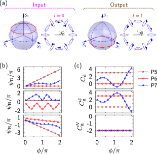
Figure 4: Transformations on vector vortex. (a) SOP trace on the Poincaré sphere and spatial distribution of SOP for input (left panel) and output (right panel) vector vortices with a designed transformation by any of optical plates P5–P7. (b) The design parameters $\{\psi_{\mathrm{D}},\psi_{\mathrm{B}},\psi_{\mathrm{R}}\}$ of Jones matrices for optical plates P5–P7 from the top down. (c) The contributions for OAM variation from dynamic term $C_{\mathrm{d}}$, geometric term $C_{\mathrm{g}}^{\mathrm{J}}$ and $C_{\mathrm{g}}^{\mathrm{V}}$ for input vector vortex shown in (a) from the top down. The contribution from $C_{\mathrm{g}}^{\mathrm{V}}$ are the same for any of P5–P7. Note that we set $I_{\mathrm{E}}(\phi)=1$.

V Discussion

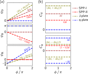
Figure 5: Features of spiral phase plates (SPPs), J-plates, and q-plates. (a) Design parameters $\{\psi_{\mathrm{D}},\psi_{\mathrm{B}},\psi_{\mathrm{R}}\}$ of Jones matrices from the top down. For SPP-I and SPP-II, the desired OAM variation is $\Delta l$ and the portion from dynamic contribution is set as $t$ for SPP-II. For J-plate, the desired OAM variation is $\Delta l_{1/2}$ for input light with left-/right-handed circular polarization. For q-plate, the desired OAM variation is $\pm\Delta l$ for input light with left-/right-handed circular polarization. (b) The corresponding dynamic (upper panel) and geometric (lower panel) contributions for OAM variation. For J-plate and q-plate, the opposite geometric contributions will be induced according to handedness of input light.

So far, there are three common optical plates—spiral phase plates, q-plates, and J-plates, which have been employed to generate and manipulate OAM beams Oemrawsingh et al. (2004); Yu et al. (2011); Devlin et al. (2017); Biener et al. (2002); Marrucci et al. (2006); Karimi et al. (2014). Actually, for all of them, the operation mechanism can be understood and explained by our theoretical approach. Here, some discussions and comments will be given. For spiral phase plates (SPPs), there are two types according to equation (5). The first one (SPP-I) is fabricated with homogeneous materials and the required phase delay is introduced by the spiral design of the plate Oemrawsingh et al. (2004). Thus, there is only the pure dynamic contribution so that the same dynamic phase, as well as the same OAM variation, can be obtained in spite of the SOP of input beams. For the second type (SPP-II), the desired OAM variation can be achieved only for a specific SOP of the input beam while the output beam would have the same SOP Yu et al. (2011). Thus, SPP-II is a particular case of P2P transformation, where the SOP of the input beam is just coincided with one of the eigen-polarizations of the plate and the SOP would be maintained. Since it just works for a specific SOP, it is not a pure dynamic phase based optical plate. Actually, for SPP-II, both the dynamic and geometric contributions have to be taken into account for the OAM variations case by case. Obviously, the operation mechanism of SPP-II is totally different with SPP-I since the OAM variation is not solely introduced by dynamic contribution.

For the J-plate Devlin et al. (2017), it could be considered as a special type of P2P transformation. The special constraint is that the orthogonal SOPs of input beam should be transferred to a flipped handedness with a different OAM variation at the same time. As shown in the inset of Fig. 1, for a J-plate, the OAM variation $\Delta l_{1}$ and $\Delta l_{2}$ should be obtained for $|b^{+}\rangle=\mathbf{J}|a^{+}\rangle$ and $|b^{-}\rangle=\mathbf{J}|a^{-}\rangle$, respectively and simultaneously. According to our framework, it means that the dynamic contributions are always the same but the geometric contributions are opposite for orthogonal input SOPs. Thus, the J-plate can be designed as that the dynamic OAM variation is $(\Delta l_{1}+\Delta l_{2})/2$ and the opposite geometric OAM variation should be $\pm(\Delta l_{1}-\Delta l_{2})/2$ according to the handedness of SOP of the input beam. Then the combinations of three parameters $\{\psi_{\mathrm{D}},\psi_{\mathrm{B}},\psi_{\mathrm{R}}\}$ can be readily obtained. Particularly, if the input field is circular polarization ($2\chi_{\mathrm{S}}=\pm\pi/2$), three parameters would hold simple relations as shown in Fig. 5(a). This kind of J-plates is a half-plate and can flip circular SOP with different OAM variations. Specifically, if $\Delta l_{1}=-\Delta l_{2}=\Delta l$, it is the well-known q-plate, in which only the pure geometric contribution is introduced Biener et al. (2002); Marrucci et al. (2006); Karimi et al. (2014) (see Appendix C for details). The full parameters of $\mathbf{J}$ for these mentioned optical plates and the corresponding contributions of each term for OAM variations are summarized and presented in Fig. 5.

As a summary, this work presents an explicit formula to evaluate the OAM variation due to the optical elements in terms of both dynamic and geometric phases. With the help of the topological Pancharatnam charge, the geometric phases can be further separated into two parts. One is directly related to optical elements and the other one solely relies on SOPs of the input and output light beams. Such treatment is not just a mathematical trick but would introduce a new viewpoint to fully understand the operation mechanism and would be helpful to explore the flexibility of designing the optical elements according to the applications. For instance, pure dynamic contribution based optical plates can implement identical OAM variations in spite of the SOP of input beam while pure geometric contribution based optical plates can serve as a mode sorter for both SAM and OAM in modern optical communication systems. Moreover, our theoretical approach can be employed for the optical systems to analyze influences due to the dynamic and geometric phases. In this work, only the case of linear orthogonal eigen-polarizations of the Jones matrix is considered since it is the common response of most materials and structures. It should be mentioned that our theoretical approach is not limited by this constraint. Actually, if the eigen-polarizations of the Jones matrix could be arbitrary, more complicated functions can be achieved for various potential applications. Additionally, there are several assumptions in our theoretical deduction such as unitary Jones matrix, paraxial beam, and fully polarized fields. Actually, breaking either of them would introduce some more interesting investigations, e.g. considering inhomogeneous Jones matrix Cerjan and Fan (2017), non-Hermitian (including PT-symmetry) systems Lawrence et al. (2014), or non-reciprocal systems Mahmoud et al. (2015). Furthermore, only classical light fields are considered in our work, but we believe that the similar work about quantum counterpart would bring more things of new physics and our work could evoke some fundamental research about spin-orbit interaction and the related topics.

Appendix A: Orbital angular momentum of an optical vortex

Under the paraxial approximation, the electric and magnetic fields of a fully polarized vector vortex beam of angular frequency $\omega$ propagating along $\mathbf{z}$ direction can be written as Torres and Torner (2011)

$$\mathbf{E}\left(x,y\right) =i\omega\left(\alpha\mathbf{\hat{x}}+\beta\mathbf{\hat{y}}+\frac{i}{k}\left(\frac{\partial\alpha}{\partial x}+\frac{\partial\beta}{\partial y}\right)\mathbf{\hat{z}}\right)e^{ikz},$$

$$\mathbf{B}\left(x,y\right) =ik\left(-\beta\mathbf{\hat{x}}+\alpha\mathbf{\hat{y}}+\frac{i}{k}\left(-\frac{\partial\beta}{\partial x}+\frac{\partial\alpha}{\partial y}\right)\mathbf{\hat{z}}\right)e^{ikz},$$

where $\alpha$ and $\beta$ represent the complex amplitude of $x-$ and $y-$component of electric field, respectively. They can be written as

$$\alpha(x,y) =\sqrt{I_{\text{E}}(x,y)}a_{x}(x,y),$$

$$\beta(x,y) =\sqrt{I_{\text{E}}(x,y)}a_{y}(x,y),$$

where $a_{x}(a_{y})=\alpha(\beta)/\sqrt{I_{\text{E}}}$ are normalized electric field components with electric intensity of $I_{\text{E}}=|\alpha|^{2}+|\beta|^{2}$. So the polarization state of this light at each site can be described by a $2\times 1$ Jones vector $\left|a\right\rangle=(a_{x},a_{y})^{\mathrm{T}}$. Then, Stokes vector $\mathbf{S}=(S_{1},S_{2},S_{3})^{\mathrm{T}}$ is defined by $S_{j}=\left\langle a|\bm{\sigma}_{j}|a\right\rangle(j=1,2,3)$, where $\bm{\sigma}_{j}$ are the Pauli matrices Gutiérrez-Vega (2011),

$$\bm{\sigma}_{1}=\begin{pmatrix}1&0\\ 0&-1\end{pmatrix},\bm{\quad}\bm{\sigma}_{2}=\begin{pmatrix}0&1\\ 1&0\end{pmatrix},\bm{\quad}\bm{\sigma}_{3}=\begin{pmatrix}0&-i\\ i&0\end{pmatrix}.$$

Meanwhile, $S_{0}=\left\langle a|\bm{\sigma}_{0}|a\right\rangle$, where $\bm{\sigma}_{0}$ equals $2\times 2$ identity matrix. Thus, for left/right circularly polarized light field $\left|\mathrm{e}_{\pm}\right\rangle=(1/\sqrt{2})(1,\pm i)^{\mathrm{T}}$, there is $S_{3}=\pm 1$. Then plotting Stokes vector $\mathbf{S}$ on three-dimensional Cartesian coordinates, the Poincaré sphere could be constructed and the corresponding azimuth ($\psi_{\mathrm{S}}$) and ellipticity ($\chi_{\mathrm{S}}$) angles are resolved by, respectively

$$\tan(2\psi_{\mathrm{S}}) =S_{2}/S_{1},$$ (A3a)

$$\sin(2\chi_{\mathrm{S}}) =S_{3}/S_{0}.$$ (A3b)

The linear momentum density, which is defined as $\mathbf{p}=\varepsilon_{0}\mathbf{E}\times\mathbf{B}$, can be expressed and divided into transverse and longitudinal components,

$$\mathbf{p}_{\bot} =i\frac{\omega\varepsilon_{0}}{2}\left[\left(\alpha\nabla\alpha^{*}+\beta\nabla\beta^{*}-\alpha^{*}\nabla\alpha-\beta^{*}\nabla\beta\right)+2\nabla\times\left(\left(\alpha^{*}\beta-\beta^{*}\alpha\right)\hat{\mathbf{z}}\right)\right],$$ (A4a)

$$\mathbf{p}_{z} =\omega k\varepsilon_{0}\left(\left|\alpha\right|^{2}+\left|\beta\right|^{2}\right)=\omega k\varepsilon_{0}I_{\text{E}}S_{0}.$$ (A4b)

Meanwhile, the energy density of such a beam is

$$w=c\mathbf{p}_{z}=\varepsilon_{0}\omega^{2}\left(\left|\alpha\right|^{2}+\left|\beta\right|^{2}\right)=\varepsilon_{0}\omega^{2}I_{\text{E}}S_{0}.$$ (A5)

Then, the cross product of linear momentum density with $\mathbf{r}$ (radius vector) gives the angular momentum density, so $z-$component of angular momentum density is

$$\mathbf{j}_{z}=\left(\mathbf{r}\times\mathbf{p}\right)_{z}=i\frac{\omega\varepsilon_{0}}{2}\left[\left(\alpha\frac{\partial}{\partial\phi}\alpha^{*}+\beta\frac{\partial}{\partial\phi}\beta^{*}-\alpha^{*}\frac{\partial}{\partial\phi}\alpha-\beta^{*}\frac{\partial}{\partial\phi}\beta\right)+2r\frac{\partial}{\partial r}\left(\alpha^{*}\beta-\beta^{*}\alpha\right)\right].$$ (A6)

Further, $\mathbf{j}_{z}$ can be divided into spin and orbital parts as

$$\mathbf{j}_{z}^{\mathrm{s}} =i\omega\varepsilon_{0}r\frac{\partial}{\partial r}\left(\alpha^{*}\beta-\beta^{*}\alpha\right)=\omega\varepsilon_{0}r\frac{\partial\left(I_{\mathrm{E}}S_{3}\right)}{\partial r},$$ (A7a)

$$\mathbf{j}_{z}^{\mathrm{o}} =i\frac{\omega\varepsilon_{0}}{2}\left(\alpha\frac{\partial}{\partial\phi}\alpha^{*}+\beta\frac{\partial}{\partial\phi}\beta^{*}-\alpha^{*}\frac{\partial}{\partial\phi}\alpha-\beta^{*}\frac{\partial}{\partial\phi}\beta\right).$$ (A7b)

With the ratio of angular momentum to energy that is examined by Allen Allen and Padgett (2000), the average SAM charge and OAM charge can be calculated as

$$\bar{s} =\omega\frac{\iint\mathbf{j}_{z}^{\text{s}}rdrd\phi}{\iint wrdrd\phi}=\frac{\iint I_{\text{E}}S_{3}rdrd\phi}{\iint I_{\text{E}}S_{0}rdrd\phi},$$ (A8a)

$$\bar{l} =\omega\frac{\iint\mathbf{j}_{z}^{\text{o}}rdrd\phi}{\iint wrdrd\phi}=\frac{\iint\mathbf{j}_{z}^{\text{o}}rdrd\phi}{\omega\epsilon_{0}\iint I_{\text{E}}S_{0}rdrd\phi}.$$ (A8b)

Then, we introduce the phase difference for two different SOPs of $\left|\mathrm{e}_{\mathrm{A}}\right\rangle$ and $\left|\mathrm{e}_{\mathrm{B}}\right\rangle$ through the Pancharatnam connection, which is defined by Berry (1987)

$$\psi_{\mathrm{P}}=\arg\left(\left\langle\mathrm{e}_{\mathrm{A}}|\mathrm{e}_{\mathrm{B}}\right\rangle\right).$$ (A9)

Here, using left/right circularly polarized fields as reference fields, the phase difference for any field $\left|a\right\rangle=(a_{x},a_{y})^{\mathrm{T}}$ can be written as

$$\psi_{\mathrm{P\pm}}=\arg\left(\left\langle\mathrm{e}_{\pm}|a\right\rangle\right).$$ (A10)

According to Ref. Zhang et al. (2015), we can obtain

$$\frac{\mathbf{j}_{z}^{\text{o}}}{\omega\epsilon_{0}I_{\text{E}}}=S_{0}\frac{\partial\psi_{\mathrm{P\pm}}}{\partial\phi}\pm(S_{0}\mp S_{3})\frac{\partial\psi_{\mathrm{S}}}{\partial\phi},$$ (A11)

then using equation (A11), we can get a relation

$$\frac{\partial\psi_{\mathrm{S}}}{\partial\phi}=-\frac{1}{2}\left(\frac{\partial\psi_{\mathrm{P+}}}{\partial\phi}-\frac{\partial\psi_{\mathrm{P-}}}{\partial\phi}\right),$$ (A12)

then equation (A11) can be rewritten as

$$\frac{\mathbf{j}_{z}^{\text{o}}}{\omega\epsilon_{0}I_{\text{E}}}=\frac{1}{2}\left((S_{0}+S_{3})\frac{\partial\psi_{\mathrm{P+}}}{\partial\phi}+(S_{0}-S_{3})\frac{\partial\psi_{\mathrm{P-}}}{\partial\phi}\right).$$ (A13)

Substituting equation (A11) or (A13) into equation (A8b), we can calculate the average OAM charge for any vortex beams. In equations (A11) and (A13), the derivative of $\psi_{\mathrm{P\pm}}$ is known as the topological Pancharatnam charge. With equation (A11), we have found that the OAM of a vector vortex can be divided into two parts: the topological Pancharatnam charge and contribution from geometric phase induced by space-variant SOP of light fields, which is consistent with the reported results Wang et al. (2010); Niv et al. (2006) and more detailed discussions were provided in our previous work Zhang et al. (2015).

Appendix B: OAM variation induced by optical elements

Here, we consider a scenario that the light beam passes through a nonabsorbing optical element and investigate the OAM variation induced by this optical element, which is characterized by a unitary Jones matrix $\mathbf{J}$ (i.e., $\mathbf{J}^{\dagger}=\mathbf{J}^{-1}$) with the eigenvalues of $\mu_{1(2)}$, eigenstates of $|q_{1(2)}\rangle$, and the corresponding Stokes vectors of $\mathbf{S}^{\mathrm{J}}=\mathbf{S}^{q_{1}}=-\mathbf{S}^{q_{2}}=(S_{1}^{\mathrm{J}},S_{2}^{\mathrm{J}},S_{3}^{\mathrm{J}})^{\mathrm{T}}$ ($S_{j}^{\mathrm{J}}=\left\langle q_{1}|\bm{\sigma}_{j}|q_{1}\right\rangle$) Gutiérrez-Vega (2011). When light field $|a\rangle$ passes through the optical element $\mathbf{J}$, the output beam can be expressed as $|b\rangle=\mathbf{J}|a\rangle$. From equation (A8b), it could be known that the variation of OAM simply depends on the variation of $\mathbf{j}_{z}^{\text{o}}$ due to non-absorbing nature ($I_{\mathrm{E}}^{a}=I_{\mathrm{E}}^{b}=I_{\mathrm{E}}$). Then with equations (A12) and (A13), the variation of $\mathbf{j}_{z}^{\text{o}}$ can be deduced as

$$\frac{\Delta\mathbf{j}_{z}^{\text{o}}}{\omega\epsilon_{0}I_{\text{E}}}=\frac{1}{2}\left((S_{3}^{b}-S_{3}^{a})\frac{\partial\psi_{\mathrm{P+}}^{a}}{\partial\phi}+(S_{0}^{b}+S_{3}^{b})\frac{\partial\psi_{\mathrm{P+}}^{a\rightarrow b}}{\partial\phi}+(S_{3}^{a}-S_{3}^{b})\frac{\partial\psi_{\mathrm{P-}}^{a}}{\partial\phi}+(S_{0}^{b}-S_{3}^{b})\frac{\partial\psi_{\mathrm{P-}}^{a\rightarrow b}}{\partial\phi}\right),$$ (A14)

where the superscript $a(b)$ refers to the parameters related to state $|a\rangle$($|b\rangle$) and $\psi_{\mathrm{P\pm}}^{a\rightarrow b}=\psi_{\mathrm{P\pm}}^{b}-\psi_{\mathrm{P\pm}}^{a}$ is the difference of phases (defined by the Pancharatnam connection) between $|a\rangle$ and $|b\rangle$. According to Refs. Gutiérrez-Vega (2011); Martínez-Fuentes et al. (2012), $\psi_{\mathrm{P\pm}}^{a\rightarrow b}$ can be written as

$$\psi_{\mathrm{P\pm}}^{a\rightarrow b}=\psi_{\mathrm{D}}-\frac{\Omega_{ab\mathrm{e}_{\pm}}^{\mathrm{C}}}{2}+\frac{\Omega_{abb^{\dagger}a^{\dagger}}^{\mathrm{J}}}{4},$$ (A15)

where $\psi_{\mathrm{D}}=\mathrm{arg}(\mu_{1}\mu_{2})/2$ is dynamic phase gained by the beam when it propagates through the optical element, $\Omega_{ab\mathrm{e}_{\pm}}^{\mathrm{C}}\big{/}2$ is the geometric phase, related to the referenced circularly polarized field, which corresponds to parallel transport of the state around a closed loop ($|a\rangle\rightarrow|b\rangle\rightarrow|\mathrm{e}_{\pm}\rangle\rightarrow|a\rangle$) on the Poincaré sphere (see Fig. 2(a) in main text), and $\Omega_{abb^{\dagger}a^{\dagger}}^{\mathrm{J}}\big{/}4$ is the geometric phase introduced by the optical element $\mathrm{\mathbf{J}}$. For the third term, $\Omega_{abb^{\dagger}a^{\dagger}}^{\mathrm{J}}$ is a spherical quadrangle corresponding to the closed trajectory $|a\rangle\rightarrow|b\rangle\rightarrow|b_{\mathrm{J}}^{\dagger}\rangle\rightarrow|a_{\mathrm{J}}^{\dagger}\rangle\rightarrow|a\rangle$, as shown in Fig. 2(b) in main text, where $|a_{\mathrm{J}}^{\dagger}\rangle(|b_{\mathrm{J}}^{\dagger}\rangle)$ holds the Stokes vector $\mathbf{S}^{a_{\mathrm{J}}^{\dagger}(b_{\mathrm{J}}^{\dagger})}=\mathbf{S}^{a(b)}-2(\mathbf{S}^{a(b)}\cdot\mathbf{S}^{\mathrm{J}})\mathbf{S}^{\mathrm{J}}$.

Further, using equations (A12) and (A15), the equation (A14) can be rewritten as

$$\frac{\Delta\mathbf{j}_{z}^{\text{o}}}{\omega\epsilon_{0}I_{\text{E}}}=S_{0}^{b}\frac{\partial\psi_{\mathrm{D}}}{\partial\phi}+S_{0}^{b}\frac{\partial}{\partial\phi}\left(\frac{\Omega_{abb^{\dagger}a^{\dagger}}^{\mathrm{J}}}{4}\right)+\left[S_{3}^{a}\frac{\partial\psi_{\mathrm{S}}^{a}}{\partial\phi}-S_{3}^{b}\frac{\partial\psi_{\mathrm{S}}^{b}}{\partial\phi}-S_{0}^{b}\frac{\partial}{\partial\phi}\left(\frac{\Omega_{abb^{\dagger}a^{\dagger}}^{\mathrm{C}}}{4}\right)\right],$$ (A16)

where $\Omega_{abb^{\dagger}a^{\dagger}}^{\mathrm{C}}$ is a spherical quadrangle defined by states $|a\rangle$, $|b\rangle$, $|b_{\mathrm{C}}^{\dagger}\rangle$ and $|a_{\mathrm{C}}^{\dagger}\rangle$ as shown in Fig. 2(b) in main text, where $|a_{\mathrm{C}}^{\dagger}\rangle(|b_{\mathrm{C}}^{\dagger}\rangle)$ holds the Stokes vector $\mathbf{S}^{a_{\mathrm{C}}^{\dagger}(b_{\mathrm{C}}^{\dagger})}=\mathbf{S}^{a(b)}-2(\mathbf{S}^{a(b)}\cdot\mathbf{S}^{\mathrm{e}_{+}})\mathbf{S}^{\mathrm{e}_{+}}$. Thus using equation (A8b), the variation of OAM charge can be solved

$$\Delta\bar{l}=\frac{\iint I_{\mathrm{E}}\Delta\mathbf{j}_{z}^{\text{o}}rdrd\phi}{\omega\epsilon_{0}\iint I_{\mathrm{E}}S_{0}^{a}rdrd\phi}.$$ (A17)

It should be noticed that equation (A17) is applicable to the transformation performed by nonabsorbing optical elements.

Note that, for any spherical triangle defined by states $|a\rangle$, $|b\rangle$ and $|c\rangle$, whose Stokes vectors are $\mathbf{S}^{a}$, $\mathbf{S}^{b}$ and $\mathbf{S}^{c}$, respectively, the triangular area $\Omega_{abc}$ is

$$\Omega_{abc}=2\mathrm{arctan}\left[\frac{\mathbf{S}^{a}\cdot(\mathbf{S}^{b}\times\mathbf{S}^{c})}{1+\mathbf{S}^{a}\cdot\mathbf{S}^{b}+\mathbf{S}^{b}\cdot\mathbf{S}^{c}+\mathbf{S}^{c}\cdot\mathbf{S}^{a}}\right].$$ (A18)

From equation (A18), it can found that clockwise and anticlockwise walks on the sphere surface will induce opposite values of solid angles. As shown in Fig. 2(b) in main text, the spherical lune is shaped by two geodesics connecting the antipodal states $|q_{1}\rangle$ and $|q_{2}\rangle$ passing through $|a\rangle$ and $|b\rangle$ and forming a dihedral angle $\psi_{\mathrm{B}}=\mathrm{arg}(\mu_{2})-\mathrm{arg}(\mu_{1})=\mathrm{arg}(\mu_{1}^{\ast}\mu_{2})$, which is introduced by birefringent of optical element (also see Fig. 6). The corresponding lune area equals $2\psi_{\mathrm{B}}=\Omega_{abq_{1}}-\Omega_{abq_{2}}$. In particular, when $|q_{1(2)}\rangle$ coincides with $|\mathrm{e}_{\pm}\rangle$, $2\psi_{\mathrm{B}}$ also equals $4(\psi_{\mathrm{S}}^{b}-\psi_{\mathrm{S}}^{a})$. It is easy to find that there is a relation $\Omega_{abb^{\dagger}a^{\dagger}}^{\mathrm{C}}=\Omega_{abq_{1}}+\Omega_{abq_{2}}$ and $\Omega_{abb^{\dagger}a^{\dagger}}^{\mathrm{J}}$ can be solved by similar approach.

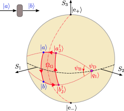
Figure 6: For the transformation from $|a\rangle$ to $|b\rangle$, there will be the introduced dynamic phase $\psi_{\mathrm{D}}$ and geometric phase $\Omega_{\mathrm{G}}/4$ by an optical element of $\{\psi_{\mathrm{D}},\psi_{\mathrm{B}}\}$ and eigen-polarizations $|q_{1(2)}\rangle$. $\Omega_{\mathrm{G}}=\Omega_{abb^{\dagger}a^{\dagger}}^{\mathrm{J}}$ is a spherical quadrangle corresponding to the closed trajectory $|a\rangle\rightarrow|b\rangle\rightarrow|b_{\mathrm{J}}^{\dagger}\rangle\rightarrow|a_{\mathrm{J}}^{\dagger}\rangle\rightarrow|a\rangle$, where $|a_{\mathrm{J}}^{\dagger}\rangle(|b_{\mathrm{J}}^{\dagger}\rangle)$ holds the Stokes vector $\mathbf{S}^{a_{\mathrm{J}}^{\dagger}(b_{\mathrm{J}}^{\dagger})}=\mathbf{S}^{a(b)}-2(\mathbf{S}^{a(b)}\cdot\mathbf{S}^{\mathrm{J}})\mathbf{S}^{\mathrm{J}}$

Appendix C: P2P Transformation on scalar vortex

1. General P2P transformation

The input scalar vortex ($|a^{+}\rangle$) is set as polarization azimuth of $\psi_{\mathrm{S}}$, ellipticity of $\chi_{\mathrm{S}}$ and carrying OAM of $l$

$$|a^{+}\rangle=e^{il\phi}\mathbf{R}(\psi_{\mathrm{S}})\left(\begin{array}[]{c}\cos(\chi_{\mathrm{S}})\\ i\sin(\chi_{\mathrm{S}})\end{array}\right),$$ (A19)

where $\mathbf{R(\cdot)}$ is the standard rotation matrix. Then using an optical element with Jones matrix $\mathbf{J}$ transfers $|a^{+}\rangle$ to the output vortex ($|b^{+}\rangle$) with a flipped handedness and OAM charge $m$ as

$$|b^{+}\rangle=e^{im\phi}\mathbf{R}(\psi_{\mathrm{S}})\left(\begin{array}[]{c}\cos(\chi_{\mathrm{S}})\\ -i\sin(\chi_{\mathrm{S}})\end{array}\right),$$ (A20)

then we can obtain the relation

$$e^{im\phi}\mathbf{R}(\psi_{\mathrm{S}})\left(\begin{array}[]{c}\cos(\chi_{\mathrm{S}})\\ -i\sin(\chi_{\mathrm{S}})\end{array}\right)=e^{il\phi}\mathbf{J}\mathbf{R}(\psi_{\mathrm{S}})\left(\begin{array}[]{c}\cos(\chi_{\mathrm{S}})\\ i\sin(\chi_{\mathrm{S}})\end{array}\right).$$ (A21)

For a scalar vortex, due to the rotation symmetry of the coordinate choice for polarization azimuth, $\psi_{\mathrm{S}}=0$ is settled for simplicity but without loss of generality, thus equation (A21) can be rewritten as

$$e^{i\Delta l_{1}\phi}\left(\begin{array}[]{c}\cos(\chi_{\mathrm{S}})\\ -i\sin(\chi_{\mathrm{S}})\end{array}\right)=\mathbf{J}\left(\begin{array}[]{c}\cos(\chi_{\mathrm{S}})\\ i\sin(\chi_{\mathrm{S}})\end{array}\right),$$ (A22)

where $\Delta l_{1}=m-l$ is the variation of OAM from $|a^{+}\rangle$ to $|b^{+}\rangle$.

Generally, without considering chiral or magneto-optic materials, $\mathbf{J}$ is linearly birefringent and the eigenstates will correspond to linearly polarized orthogonal eigen-polarizations. Being unitary, eigenvalues of $\mathbf{J}$ are given by complex exponentials of $e^{i\psi_{\mathrm{D}}}\{e^{-i\psi_{\mathrm{B}}/2},e^{i\psi_{\mathrm{B}}/2}\}$ for dynamic phase delay $\psi_{\mathrm{D}}$ and birefringent phase difference $\psi_{\mathrm{B}}$. And such two orthogonal eigen-polarizations can be written as $\mathbf{R}(\psi_{\mathrm{R}})(1,0)^{\mathrm{\mathrm{T}}}$ and $\mathbf{R}(\psi_{\mathrm{R}})(0,1)^{\mathrm{T}}$, where $\psi_{\mathrm{R}}$ is the orientation angle of eigen-polarizations. Then, for such kinds of optical elements, the Jones matrix $\mathbf{J}$ can be expressed as

$$\mathbf{J}=\left(\begin{array}[]{cc}J_{1}&J_{2}\\ J_{3}&J_{4}\end{array}\right)=e^{i\psi_{\mathrm{D}}}\left(\begin{array}[]{cc}\cos\left(\frac{\psi_{\mathrm{B}}}{2}\right)-i\sin\left(\frac{\psi_{\mathrm{B}}}{2}\right)\cos\left(2\psi_{\mathrm{R}}\right)&-i\sin\left(\frac{\psi_{\mathrm{B}}}{2}\right)\sin\left(2\psi_{\mathrm{R}}\right)\\ -i\sin\left(\frac{\psi_{\mathrm{B}}}{2}\right)\sin\left(2\psi_{\mathrm{R}}\right)&\cos\left(\frac{\psi_{\mathrm{B}}}{2}\right)+i\sin\left(\frac{\psi_{\mathrm{B}}}{2}\right)\cos\left(2\psi_{\mathrm{R}}\right)\end{array}\right).$$ (A23)

From equation (A23), it can be found that there are there parameters $\{\psi_{\mathrm{D}}(\phi),\psi_{\mathrm{B}}(\phi),\psi_{\mathrm{R}}(\phi)\}$ to determine the Jones matrix for each $\phi$, while there are just two equations to define their relations by equation (A22). The result is that we have infinite choices to construct $\mathbf{J}$ to achieve the same transformation. That is, once a contribution from dynamic phase delay $\psi_{\mathrm{D}}(\phi)$ is set, we always can find a selection of $\{\psi_{\mathrm{B}}(\phi),\psi_{\mathrm{R}}(\phi)\}$. Combining equations (A22) and (A23), we can rewrite $\mathbf{J}$

$$\mathbf{J}=e^{i\psi_{\mathrm{D}}}\left(\begin{array}[]{cc}\cos(\Delta l_{1}\phi-\psi_{\mathrm{D}})\cos(2\chi_{\mathrm{S}})+i\sin(\Delta l_{1}\phi-\psi_{\mathrm{D}})&-i\cos(\Delta l_{1}\phi-\psi_{\mathrm{D}})\sin(2\chi_{\mathrm{S}})\\ -i\cos(\Delta l_{1}\phi-\psi_{\mathrm{D}})\sin(2\chi_{\mathrm{S}})&\cos(\Delta l_{1}\phi-\psi_{\mathrm{D}})\cos(2\chi_{\mathrm{S}})-i\sin(\Delta l_{1}\phi-\psi_{\mathrm{D}})\end{array}\right).$$ (A24)

With equations (A23) and (A24), for any input light with SOP of $\chi_{\mathrm{S}}$ to obtain a desired OAM variation $\Delta l_{1}$, the design of three parameters $\{\psi_{\mathrm{D}}(\phi),\psi_{\mathrm{B}}(\phi),\psi_{\mathrm{R}}(\phi)\}$ can be solved for $\mathbf{J}$ of optical element.

To present the effect from $\{\psi_{\mathrm{D}},\psi_{\mathrm{B}}\}$ of the optical element, we give some comments and discussions on the considered transformation. As shown in Fig. 6, for the input state $\left|a\right\rangle$, we can use a geodesic arc join $\left|q_{1}\right\rangle$, $\left|a\right\rangle$ and $\left|q_{2}\right\rangle$ and let the arc go a rotation of $\psi_{\mathrm{B}}$ around the axis defined by its eigen-polarizations $|q_{1(2)}\rangle$. Then the final state $\left|b\right\rangle$ can be obtained on the corresponding location as shown in Fig. 6. From such a transformation, the introduced dynamic phase is always equal to $\psi_{\mathrm{D}}$, while the introduced geometric phase is $\Omega_{\mathrm{G}}/4=\Omega_{abb^{\dagger}a^{\dagger}}^{\mathrm{J}}\big{/}4$. It is easy to find that the geometric phase equals $-\psi_{\mathrm{B}}/2$ if $\left|a\right\rangle$=$\left|q_{1}\right\rangle$ and $\psi_{\mathrm{B}}/2$ if $\left|a\right\rangle$=$\left|q_{2}\right\rangle$. Moreover, if the input SOP is orthogonal to $\left|a\right\rangle$, i.e. the antipodal point on the Poincaré sphere, the evolution will encircle on an opposite direction but the same area using the same optical element, this means that the introduced geometric phase is $-\Omega_{\mathrm{G}}/4$ for input light with orthogonal SOP.

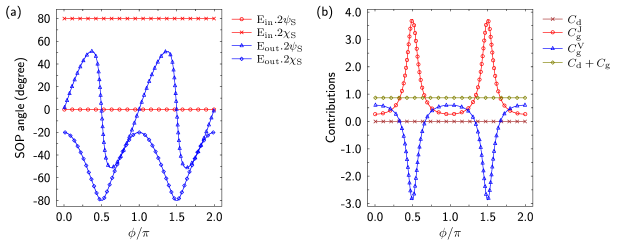
Figure 7: Transformation with P2 for input light with SOP of $\{2\psi_{\mathrm{S}},2\chi_{\mathrm{S}}\}=\{0,80^{\circ}\}$. (a) SOPs for input and output fields. (b) Detailed contributions for OAM variation from each term.

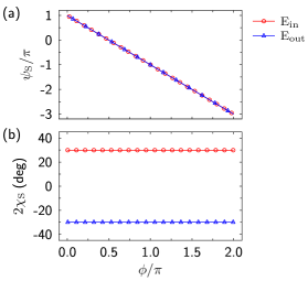
Figure 8: SOPs for input and output vector vortices shown in Fig. 4 in main text. (a) Azimuth angle $\psi_{\mathrm{S}}$ of the vector vortices. (b) Ellipticity angle $\chi_{\mathrm{S}}$ of the vector vortices.

2. J-plates and q-plates

For the J-plates Devlin et al. (2017), there is a special constrain on P2P transformation. That is, the input field with an orthogonal SOP and OAM charge of $k$ gives

$$|a^{-}\rangle=e^{ik\phi}\mathbf{R}(\psi_{\mathrm{S}})\left(\begin{array}[]{c}i\sin(\chi_{\mathrm{S}})\\ \cos(\chi_{\mathrm{S}})\end{array}\right),$$ (A25)

and the transferred output field with a flipped handedness and OAM charge of $n$, yielding

$$|b^{-}\rangle=e^{in\phi}\mathbf{R}(\psi_{\mathrm{S}})\left(\begin{array}[]{c}-i\sin(\chi_{\mathrm{S}})\\ \cos(\chi_{\mathrm{S}})\end{array}\right).$$ (A26)

With the similar approach and setting $\psi_{\mathrm{S}}=0$, we can find another relation for $\mathbf{J}$ as

$$e^{i\Delta l_{2}\phi}\left(\begin{array}[]{c}-i\sin(\chi_{\mathrm{S}})\\ \cos(\chi_{\mathrm{S}})\end{array}\right)=\mathbf{J}\left(\begin{array}[]{c}i\sin(\chi_{\mathrm{S}})\\ \cos(\chi_{\mathrm{S}})\end{array}\right),$$ (A27)

where $\Delta l_{2}=n-k$ is the variation of OAM from $|a^{-}\rangle$ to $|b^{-}\rangle$. Then, combining equations (A22) and (A27), we can get the design parameters of $\mathbf{J}$. For a special and simple case of input field with circular polarization ($2\chi_{\mathrm{S}}=\pi/2$), the combination of equations (A22) and (A27) can reduce $\mathbf{J}$ to

$$\left\{\begin{aligned} J_{1}&=-J_{4}=\frac{1}{2}\left(e^{i\Delta l_{1}\phi}-e^{i\Delta l_{2}\phi}\right)\\ J_{2}&=J_{3}=-\frac{i}{2}\left(e^{i\Delta l_{1}\phi}+e^{i\Delta l_{2}\phi}\right)\end{aligned}\right..$$ (A28)

From equation (A28), we can find the eigenvalues as

$$\left\{\begin{aligned} \mu_{1}&=i\exp\left(\frac{i(\Delta l_{1}+\Delta l_{2})\phi}{2}\right)\\ \mu_{2}&=-i\exp\left(\frac{i(\Delta l_{1}+\Delta l_{2})\phi}{2}\right)\end{aligned}\right.,$$ (A29)

and eigen-polarizations as

$$\left\{\begin{aligned} |q_{1}\rangle&=\mathbf{R}\left(\frac{(\Delta l_{1}-\Delta l_{2})\phi-\pi}{4}\right)\left(\begin{array}[]{c}1\\ 0\end{array}\right)\\ |q_{2}\rangle&=\mathbf{R}\left(\frac{(\Delta l_{1}-\Delta l_{2})\phi-\pi}{4}\right)\left(\begin{array}[]{c}0\\ 1\end{array}\right)\end{aligned}\right.,$$ (A30)

thus the parameters $\{\psi_{\mathrm{D}}(\phi),\psi_{\mathrm{B}}(\phi),\psi_{\mathrm{R}}(\phi)\}$ for $\mathbf{J}$ can be found as

$$\left\{\begin{aligned} \psi_{\mathrm{D}}(\phi)&=\frac{(\Delta l_{1}+\Delta l_{2})\phi}{2}\\ \psi_{\mathrm{B}}(\phi)&=\pi\\ \psi_{\mathrm{R}}(\phi)&=\frac{(\Delta l_{1}-\Delta l_{2})\phi-\pi}{4}\end{aligned}\right..$$ (A31)

It can be found that this kind of J-plates is a half-plate but possesses space-variant dynamic phase delay and orientation angle and can transform scalar vortices with circular polarizations. Further, q-plates would be as a special case of J-plate with opposite variation of OAM, i.e. $\Delta l_{1}=-\Delta l_{2}$. Thus, for the q-plate, there is only the contribution from geometric phases while none from dynamic phases. It should be noted that, for J-plates and q-plates, the geometric contributions actually come from the third term of equation (A16). And to calculate the OAM variation, $\psi_{\mathrm{S}}$ should be calculated using equation (A12) while not equation (A3a) due to there is a singularity for circularly polarized fields. And this singularity also induces the geometric contribution coming from $C_{\mathrm{g}}^{\mathrm{V}}$ while not $C_{\mathrm{g}}^{\mathrm{J}}$, which is different from the demonstration of P2P transformation in main text. However, this phenomenon occurs just because the circularly polarized fields are selected as the reference fields and it can be resolved if another pair of reference fields are adopted.

3. Spiral phase plates (SPPs)

Type I:

This type of spiral phase plates (SPP-I) is fabricated with homogeneous materials and can provide required phase delay by designing path length. In the transformation, only dynamic phases $\psi_{\mathrm{D}}(\phi)$ should be considered since $\psi_{\mathrm{B}}(\phi)=0$. From equation (A23), the corresponding Jones matrix for this kind of spiral phase plates can be written

$$\mathbf{J}=e^{i\psi_{\mathrm{D}}}\left(\begin{array}[]{cc}1&0\\ 0&1\end{array}\right).$$ (A32)

So they can not change the SOP but always introduce the same dynamic phase for any SOP. That is to say the same OAM variation can be achieved for any input fields.

Type II:

There is another kind of spiral phase plates (SPP-II), which can provide a desired OAM variation only for a specific SOP of input light beam and the output possessing the same SOP. Actually, the input SOP is just coincided with one of eigen-polarizations so that the dynamic or geometric phase or both of them would contribute to the OAM variations. For simplicity, we set the input SOP as $\{2\psi_{\mathrm{S}},2\chi_{\mathrm{S}}\}=\{0,0\}$ (i.e., $\psi_{\mathrm{R}}(\phi)=0$). Thus, with equation (A23), we can obtain the Jones matrix

$$\mathbf{J}=e^{i\psi_{\mathrm{D}}}\left(\begin{array}[]{cc}e^{-i\psi_{\mathrm{B}}/2}&0\\ 0&e^{i\psi_{\mathrm{B}}/2}\end{array}\right).$$ (A33)

It can found that all the contribution comes from geometric phase if $\psi_{\mathrm{D}}(\phi)=0$. For this case, the orthogonal input SOPs will get opposite OAM variations. There is another extreme case of $\psi_{\mathrm{B}}(\phi)=0$, which is exactly the SPP-I plate. Overall, this type of plates actually is a common P2P transformation plate with the same input and output SOPs.

Appendix D: Vortex beams in numerical simulations

For general vector beams, such as cylindrical vortices, the field can be expressed as

$$\mathbf{E}\left(\phi\right)=\frac{1}{\sqrt{2}}\cos\left(\frac{\pi}{4}-\chi_{\mathrm{S}}\right)(\hat{\mathbf{x}}+i\mathbf{\hat{y}})e^{i(l_{\mathrm{L}}\phi-\psi_{\mathrm{S}})}+\frac{1}{\sqrt{2}}\sin\left(\frac{\pi}{4}-\chi_{\mathrm{S}}\right)(\mathbf{\hat{x}}-i\mathbf{\hat{y}})e^{i(l_{\mathrm{R}}\phi+\psi_{\mathrm{S}})},$$ (A34)

where $l_{\mathrm{L}}$ and $l_{\mathrm{R}}$ are topological charges of field components with left- and right-handed circular polarization, respectively. With equation (A34), there is $I_{\mathrm{E}}(\phi)=1$. For a scalar vortex beam with topological charge $l$, it is easy to be obtained by setting $l_{\mathrm{L}}=l_{\mathrm{R}}=l$. For P2P transformation shown in Fig. 3(c) in the main text, we set the input light with SOP of $\{2\psi_{\mathrm{S}},2\chi_{\mathrm{S}}\}=\{0,50^{\circ}\}$ and topological charge of $l_{\mathrm{L}}=l_{\mathrm{R}}=0$ or $1$. For the transformation shown in Fig. 3(d) in the main text, we set the input light with $\{2\psi_{\mathrm{S}},2\chi_{\mathrm{S}}\}=\{0,80^{\circ}\}$ and $l_{\mathrm{L}}=l_{\mathrm{R}}=0$, where the transformation with P2 is detailed in Fig. 7. And for the transformation on vector vortex shown in Fig. 4 in the main text, we set the input light with SOP of $\{2\psi_{\mathrm{S}},2\chi_{\mathrm{S}}\}=\{2\pi-4\phi,\pi/6\}$ and topological charge of $\{l_{\mathrm{L}},l_{\mathrm{R}}\}=\{1,-3\}$, and the detailed SOPs of input and output vector vortices are presented in Fig. 8.

References

- Padgett et al. (2004) M. Padgett, J. Courtial, and L. Allen, Phys. Today 57, 35 (2004).
- Franke-Arnold et al. (2008) S. Franke-Arnold, L. Allen, and M. Padgett, Laser Photon. Rev. 2, 299 (2008).
- Barnett (2002) S. M. Barnett, J. Opt. B Quant. Semiclass. Opt. 4, S7 (2002).
- Yao and Padgett (2011) A. M. Yao and M. J. Padgett, Adv. Opt. Photon. 3, 161 (2011).
- Allen et al. (1992) L. Allen, M. W. Beijersbergen, R. J. C. Spreeuw, and J. P. Woerdman, Phys. Rev. A 45, 8185 (1992).
- Wang et al. (2010) X.-L. Wang, J. Chen, Y. Li, J. Ding, C.-S. Guo, and H.-T. Wang, Phys. Rev. Lett. 105, 253602 (2010).
- Niv et al. (2006) A. Niv, G. Biener, V. Kleiner, and E. Hasman, Opt. Express 14, 4208 (2006).
- Milione et al. (2011) G. Milione, H. I. Sztul, D. A. Nolan, and R. R. Alfano, Phys. Rev. Lett. 107, 053601 (2011).
- Milione et al. (2012) G. Milione, S. Evans, D. A. Nolan, and R. R. Alfano, Phys. Rev. Lett. 108, 190401 (2012).
- Zhang et al. (2015) D. Zhang, X. Feng, K. Cui, F. Liu, and Y. Huang, Sci. Rep. 5, 11982 (2015).
- Bliokh et al. (2008) K. Y. Bliokh, A. Niv, V. Kleiner, and E. Hasman, Nat. Photon. 2, 748 (2008).
- Bliokh et al. (2017) K. Y. Bliokh, A. Y. Bekshaev, and F. Nori, Phys. Rev. Lett. 119, 073901 (2017).
- O’Connor et al. (2014) D. O’Connor, P. Ginzburg, F. J. Rodríguez-Fortuño, G. A. Wurtz, and A. V. Zayats, Nat. Commun. 5, 5327 (2014).
- Zhao et al. (2007) Y. Zhao, J. S. Edgar, G. D. M. Jeffries, D. McGloin, and D. T. Chiu, Phys. Rev. Lett. 99, 073901 (2007).
- Onoda et al. (2004) M. Onoda, S. Murakami, and N. Nagaosa, Phys. Rev. Lett. 93, 083901 (2004).
- Hosten and Kwiat (2008) O. Hosten and P. Kwiat, Science 319, 787 (2008).
- Bliokh et al. (2015) K. Y. Bliokh, D. Smirnova, and F. Nori, Science 348, 1448 (2015).
- Bliokh et al. (2014) K. Y. Bliokh, A. Y. Bekshaev, and F. Nori, Nat. Commun. 5, 3300 (2014).
- Deng et al. (2014) Y. Deng, J. Cheng, H. Jing, and S. Yi, Phys. Rev. Lett. 112, 143007 (2014).
- Arbabi et al. (2015) A. Arbabi, Y. Horie, M. Bagheri, and A. Faraon, Nat. Nanotechnol. 10, 937 (2015).
- Yu et al. (2011) N. Yu, P. Genevet, M. A. Kats, F. Aieta, J.-P. Tetienne, F. Capasso, and Z. Gaburro, Science 334, 333 (2011).
- Marrucci et al. (2006) L. Marrucci, C. Manzo, and D. Paparo, Phys. Rev. Lett. 96, 163905 (2006).
- Bomzon et al. (2002) Z. Bomzon, G. Biener, V. Kleiner, and E. Hasman, Opt. Lett. 27, 1141 (2002).
- Devlin et al. (2017) R. C. Devlin, A. Ambrosio, N. A. Rubin, J. P. B. Mueller, and F. Capasso, Science 358, 896 (2017).
- Souza et al. (2007) C. E. R. Souza, J. A. O. Huguenin, P. Milman, and A. Z. Khoury, Phys. Rev. Lett. 99, 160401 (2007).
- Ma et al. (2016) L. B. Ma, S. L. Li, V. M. Fomin, M. Hentschel, J. B. Götte, Y. Yin, M. R. Jorgensen, and O. G. Schmidt, Nat. Commun. 7, 10983 (2016).
- Torres and Torner (2011) J. P. Torres and L. Torner, Twisted Photons: Applications of Light with Orbital Angular Momentum (John Wiley & Sons, 2011).
- Gutiérrez-Vega (2011) J. C. Gutiérrez-Vega, Opt. Lett. 36, 1143 (2011).
- Born and Wolf (2013) M. Born and E. Wolf, Principles of Optics: Electromagnetic Theory of Propagation, Interference and Diffraction of Light (Elsevier, 2013).
- Allen and Padgett (2000) L. Allen and M. J. Padgett, Opt. Commun. 184, 67 (2000).
- Bekshaev et al. (2003) A. Y. Bekshaev, M. S. Soskin, and M. V. Vasnetsov, J. Opt. Soc. Am. A 20, 1635 (2003).
- Berry (1987) M. Berry, J. Mod. Opt. 34, 1401 (1987).
- Zhao et al. (2017) P. Zhao, S. Li, Y. Wang, X. Feng, K. Cui, F. Liu, W. Zhang, and Y. Huang, Sci. Rep. 7, 7873 (2017).
- Martínez-Fuentes et al. (2012) J. L. Martínez-Fuentes, J. Albero, and I. Moreno, Opt. Commun. 285, 393 (2012).
- Oemrawsingh et al. (2004) S. S. R. Oemrawsingh, J. A. W. Van Houwelingen, E. R. Eliel, J. P. Woerdman, E. J. K. Verstegen, J. G. Kloosterboer, and G. W. t Hooft, Appl. Opt. 43, 688 (2004).
- Biener et al. (2002) G. Biener, A. Niv, V. Kleiner, and E. Hasman, Opt. Lett. 27, 1875 (2002).
- Karimi et al. (2014) E. Karimi, S. A. Schulz, I. De Leon, H. Qassim, J. Upham, and R. W. Boyd, Light Sci. Appl. 3, e167 (2014).
- Cerjan and Fan (2017) A. Cerjan and S. Fan, Phys. Rev. Lett. 118, 253902 (2017).
- Lawrence et al. (2014) M. Lawrence, N. Xu, X. Zhang, L. Cong, J. Han, W. Zhang, and S. Zhang, Phys. Rev. Lett. 113, 093901 (2014).
- Mahmoud et al. (2015) A. M. Mahmoud, A. R. Davoyan, and N. Engheta, Nat. Commun. 6, 8359 (2015).