Helium abundance and speed difference between helium ions and protons in the solar wind from coronal holes, active regions, and quiet Sun

Abstract

Two main models have been developed to explain the mechanisms of release, heating and acceleration of the nascent solar wind, the wave-turbulence-driven (WTD) models and reconnection-loop-opening (RLO) models, in which the plasma release processes are fundamentally different. Given that the statistical observational properties of helium ions produced in magnetically diverse solar regions could provide valuable information for the solar wind modelling, we examine the statistical properties of the helium abundance ($A_{He}$) and the speed difference between helium ions and protons ($v_{\alpha p}$) for coronal holes (CHs), active regions (ARs) and the quiet Sun (QS). We find bimodal distributions in the space of $A_{He}$ and $v_{\alpha p}/v_{A}$ (where $v_{A}$ is the local Alfvén speed) for the solar wind as a whole. The CH wind measurements are concentrated at higher $A_{He}$ and $v_{\alpha p}/v_{A}$ values with a smaller $A_{He}$ distribution range, while the AR and QS wind is associated with lower $A_{He}$ and $v_{\alpha p}/v_{A}$, and a larger $A_{He}$ distribution range. The magnetic diversity of the source regions and the physical processes related to it are possibly responsible for the different properties of $A_{He}$ and $v_{\alpha p}/v_{A}$. The statistical results suggest that the two solar wind generation mechanisms, WTD and RLO, work in parallel in all solar wind source regions. In CH regions WTD plays a major role, whereas the RLO mechanism is more important in AR and QS.

1 Introduction

Helium is ranked as the second most abundant element in the Sun and in the solar wind (SW), and it is an important tool in exploring the nature of the solar wind. In particular, the difference in the helium ion and proton properties can help us understand the mechanisms for the release, heating and acceleration of the nascent solar wind (e.g., Marsch et al., 1982a; Neugebauer et al., 1996; Steinberg et al., 1996; Reisenfeld et al., 2001; Kasper et al., 2007; Kasper et al., 2012). The abundance of helium ($A_{He}$) and the speed difference between helium ions and protons ($v_{\alpha p}$) in the solar wind were extensively studied in the past. The abundance of helium is about 8.5% in the photosphere (e.g., Grevesse & Sauval, 1998; Asplund et al., 2009). Measurements of the corona above polar coronal holes and surrounding quiet Sun areas showed that $A_{He}$ is in the range 4% – 5% (Laming & Feldman, 2001, 2003). The $A_{He}$ is usually below 5% in the solar wind and changes with the solar activity (Ogilvie & Hirshberg, 1974; Feldman et al., 1978). Using data obtained by WIND, Aellig et al. (2001) confirmed this finding and also established that this tendency is more clear for the slow SW. By dividing the solar wind into 25 speed intervals, Kasper et al. (2007); Kasper et al. (2012) examined the relationship between the helium abundance and the speed of the solar wind for a whole solar activity cycle, and found a strong correlation between $A_{He}$ and sunspot numbers for the slowest solar wind.

The speeds of helium ions are usually larger than the proton speeds in the solar wind, although helium ions are heavier than protons. Using data obtained by Helios, Marsch et al. (1982a) analysed the speed difference between helium ions and protons, and found that $v_{\alpha p}$ increases with the solar wind speed. While $v_{\alpha p}$ is close to the local Alfvén wave speed in the fast SW, the average $v_{\alpha p}$ for the slow SW is close to zero, and $v_{\alpha p}$ in the fast SW decreases with the increase of the heliocentric distances at almost the same rate as of $v_{A}$. Consequently, these results were confirmed from observations made by Ulysses (Neugebauer et al., 1996; Reisenfeld et al., 2001), Wind (Steinberg et al., 1996), and ACE (Berger et al., 2011).

The plasma release, heating and acceleration mechanisms of the nascent solar wind are a fundamental problem in solar and space physics. Two classes of models, the wave-turbulence-driven (WTD) models (Hollweg, 1986; Wang & Sheeley, 1991; Cranmer et al., 2007; Verdini et al., 2009) and the reconnection loop opening (RLO) models (Fisk et al., 1999; Fisk, 2003; Schwadron & McComas, 2003; Woo et al., 2004; Fisk & Zurbuchen, 2006) have been proposed to account for this. The essential difference between the two models is that the plasma escapes directly along open magnetic field lines in the WTD models, whereas in the RLO models the plasma is released by reconnection between open magnetic field lines and closed loops. Waves and turbulence are all important in the two plasma release mechanisms. In the RLO models waves originate in the reconnection process, while waves are generated by photospheric motions in the WTD models (e.g., Fisk, 2003; Cranmer et al., 2007; Cranmer, 2009; Abbo et al., 2016). Determining which physical mechanisms are at work and/or the extend of the contribution of any of the mechanisms is prerequisite for establishing physically realistic models of the solar wind and the heliosphere (Cranmer, 2009).

Generally, the solar wind is categorised by speed. However, the speed is not the only classification criterion of the solar wind (Antiochos et al., 2012; Abbo et al., 2016). The solar wind can also be differentiated by some of its in-situ measured properties, like for instance the charge state (Zhao et al., 2009; Landi et al., 2012; Zhao et al., 2014). As the charge state does not change beyond several solar radii, it carries direct information about the temperature of the source region (Owocki et al., 1983; Buergi & Geiss, 1986). Based on the in-situ properties of the proton number density, proton temperature, magnetic filed strength, and solar wind speed, Xu & Borovsky (2015) classified the solar wind into four categories, coronal-hole-origin plasma, streamer-belt-origin plasma, sector-reversal-region plasma, and ejecta. In addition, on the basis of the above four category classification, Camporeale et al. (2017) developed a solar wind classification algorithm using a Machine Learning algorithm.

The solar wind can also be classified by source regions (Neugebauer et al., 2002; Liewer et al., 2004; Fu et al., 2015, 2017; Zhao et al., 2017a, b). This is reasonable as CHs, ARs, and QS are all regarded as the sources of the solar wind, but their actual contribution is still uncertain. How the solar wind is produced in these regions is also still debatable. It is generally accepted that CHs are the sources of the solar wind (e.g., Krieger et al., 1973; Gosling & Pizzo, 1999). The solar wind can also originate from QS regions (e.g., Woo & Habbal, 2000; Feldman et al., 2005; Fu et al., 2015). Another source region of the solar wind that has been investigated in detail recent years are the edges of active regions. From the comparison of the velocity distributions at 2.5 R_⊙ and potential field extrapolations using Kitt Peak magnetograms, Kojima et al. (1999) found that low-speed wind regions are associated with large magnetic field expansions originating from area adjacent to ARs. Shortly after Winebarger et al. (2001) established the presence of intermittent flows with velocities in the range of 5 – 20  km s^-1 at the edge of an AR using data from the Transition Region and Coronal Explorer (TRACE) in the Fe ix/x 171 Å passband. With the launch of the Hinode spacecraft it became possible to further investigate these regions using imaging and spectroscopic data. Sakao et al. (2007) identified the existence of outflowing plasma at the periphery of ARs in images taken with the X-ray Telescope (XRT) on board Hinode and obtained upward Doppler velocities of $\sim$50  km s^-1 using the Extreme-ultraviolet Imaging Spectrometer (EIS) on Hinode in an Fe xii line (no wavelength is mentioned in the article). Later, Del Zanna (2008) and Harra et al. (2008) investigated these outflows obtaining upflow Doppler velocities ranging from 5 to 50  km s^-1 in coronal lines. Bryans et al. (2010) established that the outflows can be present for several days and also identified multiple velocity components in the EIS Fe xii and Fe xiii lines of up to 200  km s^-1. The follow-up finding of upflows at heights between 1.5 and 2.5 R_⊙ in the solar atmosphere using data from the Ultra-Violet Coronagraph Spectrometer on board SoHO in the H i Ly $\alpha$ and O vi doublet lines at 1031.9 Å and 1037.6 Å  (Zangrilli & Poletto, 2012) further supported the evidence that AR peripheries are a possible source of the slow SW. Several studies followed investigating both observationally and through modelling the association of AR upflows with the solar wind (He et al., 2010; van Driel-Gesztelyi et al., 2012; Culhane et al., 2014; Mandrini et al., 2014; Brooks et al., 2015; Galsgaard et al., 2015; Vanninathan et al., 2015; Zangrilli & Poletto, 2016; Baker et al., 2017).

In the present paper, we analyse $A_{He}$ and $v_{\alpha p}/v_{A}$  (where $v_{A}$ is the local Alfvén speed) of the solar wind for the three general types of solar regions, coronal holes (CHs), active regions (ARs) and the quiet Sun (QS), during three phases of the solar activity cycle. The magnetic field structures are significantly different in these three regions, with CHs generally occupied by large scale open magnetic field lines, whereas AR and QS regions are mainly taken up by closed loops (Wiegelmann & Solanki, 2004; Ito et al., 2010; Wiegelmann et al., 2014). We aim at demonstrating the differences in the properties of $A_{He}$ and $v_{\alpha p}/v_{A}$ for the three source region solar wind and during three phases of the solar cycle activity. Our expectations are that statistical observational results on the variabilities of $A_{He}$ and $v_{\alpha p}/v_{A}$ produced in magnetically diverse solar regions may provide helpful and valuable information for the solar wind modelling.

The paper is organised as follows: In Section 2, we describe the data and our method of analysis. The statistical results are presented and discussed in Section 3. Section 4 summarises the present study, ending with concluding remarks.

2 Data and Analysis

The data used in this study are all obtained by the WIND spacecraft. The proton and helium ion velocities and densities were recorded by the Solar Wind Experiment (SWE) Faraday Cup instruments (Ogilvie et al., 1995). The $A_{He}$ was obtained from the density ratio between the helium ions and protons. The magnetic field was measured by the Magnetic Field Investigation (MFI) (Lepping et al., 1995). The speed uncertainties of the solar wind are less than 0.16% (Kasper et al., 2006). In some cases, the SWE could not yield accurate helium ion measurements (Steinberg et al., 1996). First, when the proton energy-per-charge distribution is very broad, it makes the helium ion signal overpowered by the proton signal, and thus the helium ion signal cannot be extracted. Second, when the helium ion flux is unusually low, it is down the detection threshold of the detectors. Third, if the solar wind speed is too high, the helium ions may exceed the highest energy-per-charge step of SWE, thus becoming undetectable. In order to ensure accurateness, we only use data that are free of the above mentioned discrepancies. The time resolution of the data is 92 seconds. The data were averaged over 1 hr. Generally, the direction of the $v_{\alpha p}$ is assumed along the magnetic field lines (e.g., Asbridge et al., 1976; Marsch et al., 1982a; Steinberg et al., 1996; Berger et al., 2011; Reisenfeld et al., 2001). The $v_{\alpha p}$ was calculated as $v_{ap}=(v_{ra}-v_{rp})/cos(\theta)$, where $v_{ra}$ and $v_{rp}$ are the radial speed of the helium ions and protons, respectively, and $\theta$ is the angle between the radial vector and the magnetic field. In order to reduce the uncertainties, we discarded the observations in which $\theta$ is greater than 72.5 degrees ($cos(\theta)<0.3$) as done in Reisenfeld et al. (2001). The $v_{\alpha p}$ is usually compared with the local Alfvén speed ($v_{A}$; Marsch et al., 1982a; Steinberg et al., 1996; Berger et al., 2011; Reisenfeld et al., 2001) which was calculated as $v_{A}=22.3*B_{rtn}/\sqrt{(n_{p}+4*n_{a})}$, where $B_{rtn}$, $n_{p}$, and $n_{a}$ are the magnetic filed strength in nT, and density of proton and helium ions in number per cubic centimetre (n/cc). At last, $v_{\alpha p}$ was divided by $v_{A}$.

For completeness, we repeat here the description of the two-step mapping procedure (Neugebauer et al., 1998; Neugebauer et al., 2002; Liewer et al., 2004) that was used in tracing the solar wind back to the solar surface (already described in Fu et al. (2015, 2017)). First, each solar wind parcel is traced back in a ballistic approach to the source surface which is implemented by the coronal magnetic field model. Second, the wind parcel is traced from the source surface to the photosphere by following the magnetic filed lines computed by a potential field source surface (PFSS) model (Schatten et al., 1969; Altschuler & Newkirk, 1969). The footpoints of the solar wind parcels were then placed on the photospheric magnetograms obtained with the Michelson Doppler imager (MDI, Scherrer et al., 1995) and the EUV images taken by the Extreme-ultraviolet Imaging Telescope (EIT, Delaboudinière et al., 1995) on board Solar and Heliospheric Observatory (SoHO, Domingo et al., 1995). The regions with the located footpoints were then categorised into three groups. The solar wind was named by the three type of source regions they originate from, CH, AR, or QS wind.

The categorisation scheme is demonstrated in Figure 1. The footpoint locations are overplotted on the EIT 284 Å images (a1, b1, c1, d1) and MDI magnetograms (a2, b2, c2, d2) marked by red crosses. The classification of the source regions relies on the coronal hole and magnetically concentrated area boundaries. The wind is classified as CH wind if its footpoints are located within the CH boundaries. An AR wind is defined if its footpoints fall in a magnetically concentrated area which is a numbered NOAA AR. When a footpoint is positioned out of any CH and magnetically concentrated area, it is then marked as a QS wind. More details on how the boundaries are determined, as well as the classification of the source regions and the tracing back procedure, can be found in Fu et al. (2015, 2017).

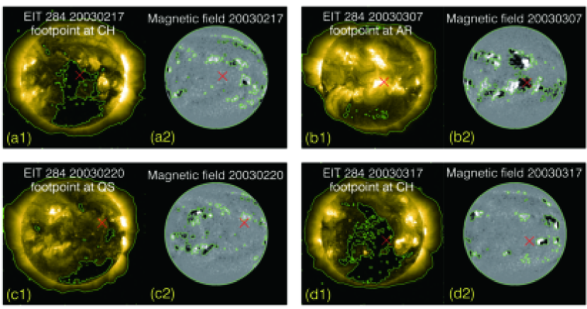
Figure 1: Illustration of the classification scheme of the solar wind. EIT 284 Å images (a1, b1, c1, d1) and corresponding photospheric magnetograms (a2, b2, c2, d2) are shown. The green contours outline the CHs and magnetically concentrated area boundaries. The footpoints are represented by red crosses.

The intervals occupied by Interplanetary Coronal Mass Ejections (ICMEs) were discarded where the charge states O⁷⁺/O⁶⁺ exceed $6.008exp(-0.00578v)$, where $v$ is the ICME speed in km s^-1 (Richardson & Cane, 2004). The daily averaged solar wind velocity was used in tracing the solar wind back to the source surface, therefore one footpoint for each day is determined. The data used here cover the years from 2000 to 2008. This time period covers the solar maximum (2000 – 2001, hereafter MAX), the decline (2002 – 2006, DEC), and the minimum phases (2007 – 2008, MIN) of cycle 23. The statistical results are based on the following number of measurements. For the full speed range (Figure 3), the hourly in-situ samples of the solar wind are 2844, 694, 1634, and 516 for the solar wind as a whole, CH, AR, and QS wind during solar maximum, respectively. The hourly in-situ samples of the solar wind are 6362, 2340, 2282, and 1740, respectively during DEC, and 2169, 635, 352, 1182 during the MIN phase.

3 Results and discussion

3.1 Full speed range solar wind

Figure 2 presents the scatter (left panel) and contour (right panel) plots of the solar wind measurements in speed, $A_{He}$, and $v_{\alpha p}/v_{A}$ space. Clearly, the solar wind as a whole is separated into two main parts in the three-dimensional space which is more evident from the contour plots. One part lies in the region of higher $A_{He}$ and $v_{\alpha p}/v_{A}$, and a wider speed range, coming mainly from CHs. In contrast, the other part has lower values of $A_{He}$, $v_{\alpha p}/v_{A}$, and a wider $A_{He}$ range, that mainly originates from AR and QS regions. The quantitative analyses of $A_{He}$ and $v_{\alpha p}/v_{A}$ for the three source region solar wind are given in the following.

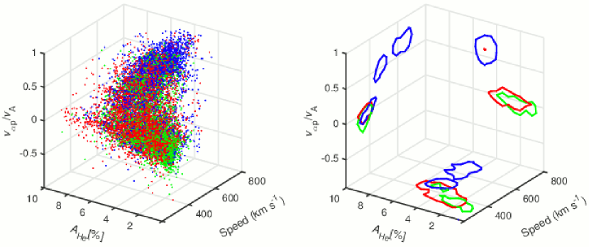
Figure 2: Scatter (left panel) and contour (right) plots of the solar wind in speed, $A_{He}$, and $v_{\alpha p}/v_{A}$ space. Blue, red, and green represent the wind from CH, AR, and QS regions, respectively. The contours correspond to 50% of the maximum counts for different source region solar wind.

Figure 3 (first column) shows the measurements of $A_{He}$ vs $v_{\alpha p}/v_{A}$ for the solar wind as a whole. The ranges of $A_{He}$ (0 – 10) and $v_{\alpha p}/v_{A}$ ($-$1.0 – 1.0) are divided into 20 parts. This means that delta $A_{He}$ and delta $v_{\alpha p}/v_{A}$ are 0.5 and 0.1, respectively, and the space of $A_{He}$ and $v_{\alpha p}/v_{A}$ is divided into 400 subsections. We also made estimations of the $A_{He}$ vs $v_{\alpha p}/v_{A}$  for each individual source region, namely, CH, AR and QS (second, third and fourth columns, respectively) that make the total contribution in the first column of Figure 3. The results are also obtained for the three solar cycle phases, the MAX, the DEC, and the MIN as the $A_{He}$ is known to change with the solar cycle activity (Aellig et al., 2001; Kasper et al., 2007; Kasper et al., 2012). The solar wind as a whole (first column in Figure 3) has a bimodal distribution in the $A_{He}$ and $v_{\alpha p}/v_{A}$ space. In order to give a quantitative evaluation of the two peaks of the distribution, we estimated the proportions of the count measurements of $A_{He}$ and $v_{\alpha p}/v_{A}$  averaged over 1 hr located inside the 50% contour lines of the solar wind as a whole. One of the peaks of this distribution lies in the range of higher $A_{He}$ and $v_{\alpha p}/v_{A}$ (hereafter H$\_$av) and has proportions of 25%, 33%, and 26% of the total counts for the solar MAX, DEC and MIN. The proportions are given in each panel of Figure 3. In H$\_$av the $A_{He}$ ranges are 3.75 – 5.75, 3.75 – 5.75, and 3.5 – 5.25, and the $v_{\alpha p}$ ranges are 0.3 – 0.7, 0.3 – 0.8, and 0.2 – 0.7, respectively. In contrast, the other peak covers lower values of $A_{He}$ and $v_{\alpha p}/v_{A}$  with contributions of 48%, 27%, and 34% during the MAX, DEC, and MIN (hereafter L$\_$av). The corresponding $A_{He}$ ranges are 1.25 – 5.50, 1.00 – 3.75, and 0.25 – 3.00, while the $v_{\alpha p}$ ranges are $-$0.3 – 0.2, $-$0.2 – 0.1, and $-$0.2 – 0.1. It is notable that the $A_{He}$ distribution ranges of H$\_$av are narrower than the ranges of L$\_$av, 2.0 vs 4.25, 2.0 vs 2.75, and 1.75 vs 2.75, during the MAX, DEC and MIN, respectively. We note that Bourouaine et al. (2011) have also obtained a bimodal distribution in the $A_{He}$ and $v_{\alpha p}/v_{A}$ space. However, the difference from their study (see their Figure 3) is that we give the distributions for the solar wind originating from various source regions.

We then estimated the count contributions of H$\_$av and L$\_$av for each of the solar wind source regions by applying the same $A_{He}$ and $v_{\alpha p}/v_{A}$ ranges as estimated from the whole Sun bimodal distribution. A noticeable finding here is that the CH wind counts are concentrated in the H$\_$av (Figure 3, second column). The lower limit contributions of H$\_$av are much higher than those of L$\_$av for CH wind. In contrast, for the AR and QS wind the proportions of L$\_$av are much higher than H$\_$av (Figure 3, third and fourth column). Thus, the AR and the QS wind counts are predominantly located in the L$\_$av.

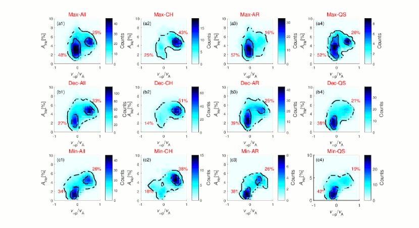
Figure 3: Contour plots of the solar wind originating in CH, AR, and QS regions in the $A_{He}$ and $v_{\alpha p}/v_{A}$ space. The first to fourth columns correspond to the wind as a whole, and from CH, AR, and QS regions, respectively. The top, middle, and bottom panels represent the solar maximum, decline, and minimum phases. The percentages of the samples located in the concentrations of higher $A_{He}$ and $v_{\alpha p}/v_{A}$ values (H$\_$av) and lower $A_{He}$ and $v_{\alpha p}/v_{A}$ values (L$\_$av) are also given. The solid line contour corresponds to 50% and the outer contour to 10%.

How the results change if the three types (CH, AR, and QS) solar wind are determined more restrictively? Usually the footpoints of the solar wind stay in a particular region for a few days (as shown in Figure 1 of Fu et al. (2017)). A boundary wind is defined when the footpoint of the solar wind moves from one region to another (Neugebauer et al., 2002). Here, if the footpoint is located at the same region for more than 2 days, the solar wind associated with the first and last 12 hours, between the change of the footpoint location is defined as a boundary wind. This way only the core wind for a certain region can be extracted. As expected, the samples of the data become smaller. However, the distribution characteristics of the core solar wind are almost the same as in the original selection scheme. The only clear difference is that the proportions of L$\_$av decrease for the CH wind.

Several studies indicate that the solar wind produced by the WTD mechanism has higher $A_{He}$ and $v_{\alpha p}$, while the solar wind may have lower $A_{He}$ and $v_{\alpha p}$ when the RLO mechanism is at work. While it is challenging to obtain direct observations of the $A_{He}$  in the solar corona, first ionisation potential (FIP) bias measurements are more readily available. It is found that generally the FIP bias is higher in AR and QS regions (mainly occupied by closed loops) than in CH regions (generally taken up by open magnetic field lines) (Widing & Feldman, 2001; Feldman et al., 2005; Brooks & Warren, 2011; Baker et al., 2013). It is believed that the reason for the enrichment of the low FIP ions in the corona and the solar wind is that they are ionized earlier in comparison to high FIP elements. The helium has the highest FIP and remains neutral longest. This results in the enrichment/depletion of low FIP elements/helium because only ions interact with waves (Laming, 2012, 2015, 2017). It means that the helium abundance should be inversely proportional to the low FIP bias elements in the corona. Thus, the $A_{He}$ is higher in open magnetic field structures and lower in closed loops if the above mechanism is valid. The helium abundance for the fast SW coming from large CHs is higher and remarkably stable (Schwenn, 2006). In contrast, Rakowski & Laming (2012) suggested that the helium is depleted in closed loops and the depletion efficiency is higher in larger loops, and lower in smaller loops. Furthermore, from simulations, Laming (2017) showed that the $A_{He}$ is higher in open magnetic field regions and it is lower in closed loops. Suess et al. (2009) found that the solar wind that comes from big streamers has lower helium abundance. The solar wind can be produced by interchange reconnection in the streamers (Huang et al., 2016). This gives the observational support to the notion that the $A_{He}$ is lower in the closed loops as streamer structures are composed by very large closed loops.

As already mentioned, the speeds of helium ions are usually larger than protons, although the helium ions are heavier than protons. Generally, it is believed that the helium ions are heated by resonant wave-particle interactions (e.g., Hollweg & Turner, 1978; McKenzie & Marsch, 1982; Isenberg, 1984) with waves preferentially heating the heavy ions, making them faster than protons. This means that the wave acceleration is the reason why there is a speed difference between helium ions and protons (Cranmer et al., 2008). The fact that $v_{\alpha p}$ decreases with heliocentric distances (Marsch et al., 1982a; Neugebauer et al., 1996; Reisenfeld et al., 2001) suggests that the speed difference between the helium ions and protons is produced near the Sun. Therefore, it supports the idea that the wave super-acceleration of helium ions takes place near the Sun, possibly in the region of acceleration of the solar wind (Neugebauer et al., 1996). For the solar wind that escapes directly along open magnetic field lines, the wave accelerated solar wind starts from the chromosphere, whereas the solar wind released from closed loops is initiated higher in the solar atmosphere. It is possible that the solar wind that escapes directly along open magnetic field lines has more time to make a speed difference compared with the wind released from loops. This speculation, however, needs to be further supported by modeling. The above effects indicate that the wind that escapes directly along open magnetic field lines (treated by the WTD models) has larger $v_{\alpha p}$, whereas the solar wind released from closed loops (e.g., RLO models) has smaller $v_{\alpha p}$ (Stakhiv et al., 2016).

However, the $v_{\alpha p}$ will also be affected in the following propagation process. First, it is constrained by various instabilities such as the Alfvén/ion-cyclotron and fast-magnetosonic/whistler instabilities (Bourouaine et al., 2013). Qualitatively, those instabilities are only valid when the $v_{\alpha p}$ nears or exceeds the local Alfvén speed (Li & Habbal, 2000; Verscharen & Chandran, 2013; Lu et al., 2009), therefore they have smaller effect on the solar wind with small $v_{\alpha p}/v_{A}$. Second, collisions can reduce $v_{\alpha p}$ in the solar wind (e.g., Marsch et al., 1982b; Kasper et al., 2008). Bourouaine et al. (2011) found a general inverse relationship between the $v_{\alpha p}/v_{A}$ and collisional age, which means the collisions are important. This should be more significant for the slow SW which has higher collisional age. However, the distribution range in collisional age and $v_{\alpha p}/v_{A}$ space are very large (Figure 2 (b) in Bourouaine et al.,2011) which indicates that $v_{\alpha p}$ may still persist in part of the slow speed SW (speed less than 500 km s^-1). Here, the distributions in $A_{He}$ and $v_{\alpha p}/v_{A}$ space for the intermediate SW (with speed greater than 400 km s^-1 and less than 500 km s^-1) demonstrate that a higher $v_{\alpha p}/v_{A}$  at $\sim$0.4 could still be found in the solar wind whose speed is less than 500 km s^-1 (see Section 3.2 and Figure 5 below for justifications).

Fu et al. (2017) suggested that the two-peak distribution of CH wind and the anti-correlation between the speed and O⁷⁺/O⁶⁺ can be explained qualitatively by both the WTD and RLO models, implying that the combination of the two classes of mechanisms may be at work (Cranmer, 2009). The clear bimodal distribution in space of $A_{He}$ and $v_{\alpha p}/v_{A}$ for the solar wind as a whole (Figure 2 and the first column of Figure 3) can also result from the interplay of the direct plasma release mechanism along open magnetic field lines treated by the WTD models and via reconnection between closed and open fields in the RLO models. This is consistent with the idea that the WTD and RLO scenarios do not need to be ‘mutually exclusive with each other’ as suggested by Cranmer (2009) and Abbo et al. (2016).

The distributions in space of $A_{He}$ and $v_{\alpha p}/v_{A}$ for the solar wind that originates from various source regions (the second to fourth columns of Figure 3) provide additional support to the notion that possibly the WTD and RLO mechanisms work together. Spectroscopic observations have shown that there exists a stable outflow at the base of CH regions (Hassler et al., 1999; Xia et al., 2003, 2004; Tu et al., 2005) and the outflow usually corresponds to concentrations of unipolar magnetic fields (Xia et al., 2003, 2004) where the open magnetic field lines are rooted. On the other hand, closed loops dominate in ARs and QS, and therefore, the solar wind plasma is more likely to be released by magnetic reconnection between closed loops and open magnetic field lines (Neugebauer et al., 2002; Feldman et al., 2005; Harra et al., 2008; He et al., 2010; Zangrilli & Poletto, 2012; van Driel-Gesztelyi et al., 2012; Culhane et al., 2014; Mandrini et al., 2014; Baker et al., 2017).

The low count number at L$\_$av and H$\_$av for the three types solar wind can also be explained reasonably by the above suggestion. For the CH wind (Figure 3, second column) these L$\_$av measurements could be interpreted as related to magnetic reconnection between open magnetic field lines and loops along CH boundaries, as well as loops associated with small magnetic bipoles, in particular with the emergence of ephemeral regions. In ARs (Figure 3, third column), a low count H$\_$av is possibly related to small-scale coronal holes adjacent to ARs which are often obscured by overlying large loops coming out of the ARs (e.g., Wang, 2017). The domination of L$\_$av in the QS is logical as this region is predominately seeded by closed loops. The existence of open field lines in QS regions explains the presence of H$\_$av counts that are smaller but still significant (Woo & Habbal, 1997; Habbal et al., 1997; Woo & Habbal, 2000).

The observational results for the $A_{He}$ distribution ranges of H$\_$av and L$\_$av in Figure 3 can be reasonably interpreted as an interplay of the WTD and RLO mechanisms as suggested above. The $A_{He}$ distribution ranges are smaller for the H$\_$av (2.00, 2.00, and 1.75 during MAX, DEC, and MIN) compared with the L$\_$av (4.25, 2.75, and 2.75). The simulations by Rakowski & Laming (2012) have shown that closed loops show a depletion effect on helium ions, and the depletion efficiency is higher in larger loops and lower in smaller loops. Therefore, the distributions of $A_{He}$ are shifted towards lower values and the distribution ranges are wider for the L$\_$av for regions populated by larger loops (e.g., Wiegelmann & Solanki, 2004; Feldman et al., 2005).

3.2 Slow, intermediate, and fast solar wind

The results for the solar wind in full speed range (Figure 3), show a clear bimodal distribution denoted as H$\_$av and L$\_$av. Generally, the solar wind is divided into two categories, fast and slow SW, and two thresholds are usually chosen, 400 km s^-1 (e.g. Schwenn, 2006) or 500 km s^-1 (e.g. Fu et al., 2015; Stakhiv et al., 2016; Fu et al., 2017). To separate the distribution characteristics of Figure 2, we divided the solar wind into three categories, slow SW (speed of less than 400 km s^-1), intermediate SW (speed greater than 400 km s^-1 and less than 500 km s^-1), and fast SW (greater than 500 km s^-1). To explore the distribution characteristics of the solar wind in different speed ranges for the three source regions, we produced distributions in $A_{He}$ and $v_{\alpha p}/v_{A}$ space for the slow SW, intermediate SW, and fast SW given in Figure 4, Figure 5, and Figure 6, respectively.

Figure 4 shows the distributions in $A_{He}$ and $v_{\alpha p}/v_{A}$ space for the slow SW only. The proportions of L$\_$av are much higher than that of H$\_$av (generally far below 10%, except for CHs). The measurements for the slow SW are mainly concentrated at lower $A_{He}$ and $v_{\alpha p}/v_{A}$ values with wider $A_{He}$ distribution ranges for all three types slow SW. In contrast, the fast SW (Figure 6) is mainly distributed at higher $A_{He}$ and $v_{\alpha p}/v_{A}$ values with narrower $A_{He}$ distribution ranges for all three types fast SW. The difference in the proportions of H$\_$av and L$\_$av for the intermediate SW are obvious comparing the slow SW (dominant L$\_$av) and fast SW (dominant H$\_$av). H$\_$av and L$\_$av are both present in all three types intermediate SW (Figure 5), with H$\_$av that is dominant during the MAX and DEC phases for the whole SW. In general, the distributions for the intermediate SW are more complex than for the slow SW and fast SW which could be seen in Figure 5, second (CHs), third (ARs), and fourth column (QS). As we suggested, the L$\_$av is produced by the RLO mechanism, whereas the H$\_$av associates with the WTD mechanism. Our results indicate that the slow SW is mainly produced by the RLO mechanism, in contrast the fast SW is mainly generated by the WTD regardless of the source types of the solar wind. The WTD and RLO mechanisms are both present in the intermediate SW, with a different input of each mechanism for the different source regions and during different phases of the solar cycle activity. The L$\_$av for the AR region solar wind is most probably related to AR edge outflows (see Sect. 1) released into the solar wind through magnetic reconnection of the AR loops and open magnetic field lines of adjacent CHs.

Based on in-situ observations, Stakhiv et al. (2016) suggested that the solar wind with a speed of less than 500 km s^-1 can be divided into two types, one that is alike the fast SW and the other originating from closed loops. It is clear that the fast SW and “the wind originating from closed loops” in Stakhiv et al. (2016) can be associated with both the WTD and RLO mechanisms. Based on the present statistical results, an interplay of the WTD and RLO mechanisms is present for the solar wind of less than 500  km s^-1. Therefore, our results give the observational support to the suggestion of Stakhiv et al. (2016).

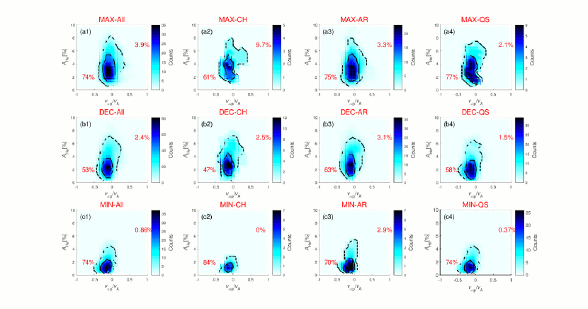
Figure 4: As in Figure 3, but for the slow SW only.

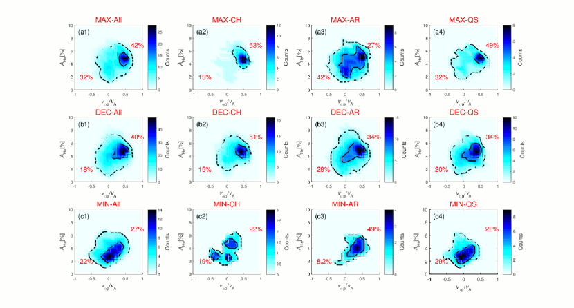
Figure 5: As in Figure 3, but for the intermediate SW only.

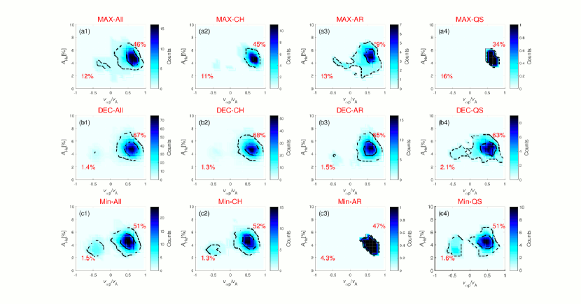
Figure 6: As in Figure 3, but for the fast SW only.

4 Summary and concluding remarks

The main purpose of the present work was to examine the statistical properties of the $A_{He}$ and $v_{\alpha p}/v_{A}$ and their distributional characteristics in space of $A_{He}$ and $v_{\alpha p}/v_{A}$ for three source region solar wind, CHs, ARs and QS. The main results are summarised as follows:

1. We found bimodal distributions of the solar wind as a whole in the $A_{He}$ and $v_{\alpha p}/v_{A}$ space. One peak lies in the range of higher values of $A_{He}$ and $v_{\alpha p}/v_{A}$. In contrast, the other peak is located at lower values of $A_{He}$ and $v_{\alpha p}/v_{A}$. The analysis for the three source region solar wind shows that the CH wind counts are concentrated at higher $A_{He}$ and $v_{\alpha p}/v_{A}$ values with narrower $A_{He}$ distribution ranges, while the AR and QS wind is mainly located at lower $A_{He}$ and $v_{\alpha p}/v_{A}$ with larger $A_{He}$ distribution ranges.

2. Almost all of the slow SW (fast SW) measurements are concentrated at lower (higher) $A_{He}$ and $v_{\alpha p}/v_{A}$ values with wider (narrower) $A_{He}$ distribution ranges regardless of the source region type. In contrast, the H$\_$av and L$\_$av are both present in all three types (CH, AR, and QS) intermediate SW.

The results demonstrate that there are clear differences of $A_{He}$ and $v_{\alpha p}/v_{A}$ for the three source region solar wind. This indicates that the configuration of the magnetic field has influence on the $A_{He}$ and $v_{\alpha p}/v_{A}$ properties. We suggest that the two solar wind generation mechanisms, the wave-turbulence-driven (WTD) and the reconnection-loop opening (RLO), work in parallel in all solar wind source regions. In CH regions WTD plays a major role, whereas RLO is more important in AR and QS regions.

The statistical results for different speed range solar wind indicate that the slow SW (speed less than 400 km s^-1) is mainly produced by the RLO mechanism, in contrast the fast SW (speed greater than 500 km s^-1) is mainly generated by the WTD mechanism regardless of the source types of the solar wind. Whereas both the WTD and RLO mechanisms play role for the generation of the intermediate SW (speed range 400 – 500 km s^-1).

The future Solar Orbiter mission that comes as close as 0.285 AU to the Sun should help reduce the uncertainties in tracing the solar wind back to the Sun and thus bring more accurate evaluation of the properties of $A_{He}$ and $v_{\alpha p}$ for different source region solar wind.

References

- Abbo et al. (2016) Abbo L., et al., 2016, Space Sci. Rev., 201, 55
- Aellig et al. (2001) Aellig M. R., Lazarus A. J., Steinberg J. T., 2001, Geophys. Res. Lett., 28, 2767
- Altschuler & Newkirk (1969) Altschuler M. D., Newkirk G., 1969, Sol. Phys., 9, 131
- Antiochos et al. (2012) Antiochos S. K., Linker J. A., Lionello R., Mikić Z., Titov V., Zurbuchen T. H., 2012, Space Sci. Rev., 172, 169
- Asbridge et al. (1976) Asbridge J. R., Bame S. J., Feldman W. C., Montgomery M. D., 1976, J. Geophys. Res., 81, 2719
- Asplund et al. (2009) Asplund M., Grevesse N., Sauval A. J., Scott P., 2009, ARA&A, 47, 481
- Baker et al. (2013) Baker D., Brooks D. H., Démoulin P., van Driel-Gesztelyi L., Green L. M., Steed K., Carlyle J., 2013, ApJ, 778, 69
- Baker et al. (2017) Baker D., Janvier M., Démoulin P., Mandrini C. H., 2017, Sol. Phys., 292, 46
- Berger et al. (2011) Berger L., Wimmer-Schweingruber R. F., Gloeckler G., 2011, Physical Review Letters, 106, 151103
- Bourouaine et al. (2011) Bourouaine S., Marsch E., Neubauer F. M., 2011, ApJ, 728, L3
- Bourouaine et al. (2013) Bourouaine S., Verscharen D., Chandran B. D. G., Maruca B. A., Kasper J. C., 2013, ApJ, 777, L3
- Brooks & Warren (2011) Brooks D. H., Warren H. P., 2011, ApJ, 727, L13
- Brooks et al. (2015) Brooks D. H., Ugarte-Urra I., Warren H. P., 2015, Nature Communications, 6, 5947
- Bryans et al. (2010) Bryans P., Young P. R., Doschek G. A., 2010, ApJ, 715, 1012
- Buergi & Geiss (1986) Buergi A., Geiss J., 1986, Sol. Phys., 103, 347
- Camporeale et al. (2017) Camporeale E., Carè A., Borovsky J. E., 2017, Journal of Geophysical Research (Space Physics), 122, 10
- Cranmer (2009) Cranmer S. R., 2009, Living Reviews in Solar Physics, 6, 3
- Cranmer et al. (2007) Cranmer S. R., van Ballegooijen A. A., Edgar R. J., 2007, ApJS, 171, 520
- Cranmer et al. (2008) Cranmer S. R., Panasyuk A. V., Kohl J. L., 2008, ApJ, 678, 1480
- Culhane et al. (2014) Culhane J. L., et al., 2014, Sol. Phys., 289, 3799
- Del Zanna (2008) Del Zanna G., 2008, A&A, 481, L49
- Delaboudinière et al. (1995) Delaboudinière J.-P., et al., 1995, Sol. Phys., 162, 291
- Domingo et al. (1995) Domingo V., Fleck B., Poland A. I., 1995, Sol. Phys., 162, 1
- Feldman et al. (1978) Feldman W. C., Asbridge J. R., Bame S. J., Gosling J. T., 1978, J. Geophys. Res., 83, 2177
- Feldman et al. (2005) Feldman U., Landi E., Schwadron N. A., 2005, Journal of Geophysical Research (Space Physics), 110, A07109
- Fisk (2003) Fisk L. A., 2003, Journal of Geophysical Research (Space Physics), 108, 1157
- Fisk & Zurbuchen (2006) Fisk L. A., Zurbuchen T. H., 2006, Journal of Geophysical Research (Space Physics), 111, A09115
- Fisk et al. (1999) Fisk L. A., Schwadron N. A., Zurbuchen T. H., 1999, J. Geophys. Res., 104, 19765
- Fu et al. (2015) Fu H., Li B., Li X., Huang Z., Mou C., Jiao F., Xia L., 2015, Sol. Phys., 290, 1399
- Fu et al. (2017) Fu H., Madjarska M. S., Xia L., Li B., Huang Z., Wangguan Z., 2017, ApJ, 836, 169
- Galsgaard et al. (2015) Galsgaard K., Madjarska M. S., Vanninathan K., Huang Z., Presmann M., 2015, A&A, 584, A39
- Gosling & Pizzo (1999) Gosling J. T., Pizzo V. J., 1999, Space Sci. Rev., 89, 21
- Grevesse & Sauval (1998) Grevesse N., Sauval A. J., 1998, Space Sci. Rev., 85, 161
- Habbal et al. (1997) Habbal S. R., Woo R., Fineschi S., O’Neal R., Kohl J., Noci G., Korendyke C., 1997, ApJ, 489, L103
- Harra et al. (2008) Harra L. K., Sakao T., Mandrini C. H., Hara H., Imada S., Young P. R., van Driel-Gesztelyi L., Baker D., 2008, ApJ, 676, L147
- Hassler et al. (1999) Hassler D. M., Dammasch I. E., Lemaire P., Brekke P., Curdt W., Mason H. E., Vial J.-C., Wilhelm K., 1999, Science, 283, 810
- He et al. (2010) He J.-S., Marsch E., Tu C.-Y., Guo L.-J., Tian H., 2010, A&A, 516, A14
- Hollweg (1986) Hollweg J. V., 1986, J. Geophys. Res., 91, 4111
- Hollweg & Turner (1978) Hollweg J. V., Turner J. M., 1978, J. Geophys. Res., 83, 97
- Huang et al. (2016) Huang J., Liu Y. C.-M., Klecker B., Chen Y., 2016, Journal of Geophysical Research (Space Physics), 121, 19
- Isenberg (1984) Isenberg P. A., 1984, J. Geophys. Res., 89, 6613
- Ito et al. (2010) Ito H., Tsuneta S., Shiota D., Tokumaru M., Fujiki K., 2010, ApJ, 719, 131
- Kasper et al. (2006) Kasper J. C., Lazarus A. J., Steinberg J. T., Ogilvie K. W., Szabo A., 2006, Journal of Geophysical Research (Space Physics), 111, A03105
- Kasper et al. (2007) Kasper J. C., Stevens M. L., Lazarus A. J., Steinberg J. T., Ogilvie K. W., 2007, ApJ, 660, 901
- Kasper et al. (2008) Kasper J. C., Lazarus A. J., Gary S. P., 2008, Physical Review Letters, 101, 261103
- Kasper et al. (2012) Kasper J. C., Stevens M. L., Korreck K. E., Maruca B. A., Kiefer K. K., Schwadron N. A., Lepri S. T., 2012, ApJ, 745, 162
- Kojima et al. (1999) Kojima M., Fujiki K., Ohmi T., Tokumaru M., Yokobe A., Hakamada K., 1999, J. Geophys. Res., 104, 16993
- Krieger et al. (1973) Krieger A. S., Timothy A. F., Roelof E. C., 1973, Sol. Phys., 29, 505
- Laming (2012) Laming J. M., 2012, ApJ, 744, 115
- Laming (2015) Laming J. M., 2015, Living Reviews in Solar Physics, 12, 2
- Laming (2017) Laming J. M., 2017, ApJ, 844, 153
- Laming & Feldman (2001) Laming J. M., Feldman U., 2001, ApJ, 546, 552
- Laming & Feldman (2003) Laming J. M., Feldman U., 2003, ApJ, 591, 1257
- Landi et al. (2012) Landi E., Alexander R. L., Gruesbeck J. R., Gilbert J. A., Lepri S. T., Manchester W. B., Zurbuchen T. H., 2012, ApJ, 744, 100
- Lepping et al. (1995) Lepping R. P., et al., 1995, Space Sci. Rev., 71, 207
- Li & Habbal (2000) Li X., Habbal S. R., 2000, J. Geophys. Res., 105, 7483
- Liewer et al. (2004) Liewer P. C., Neugebauer M., Zurbuchen T., 2004, Sol. Phys., 223, 209
- Lu et al. (2009) Lu Q., Du A., Li X., 2009, Physics of Plasmas, 16, 042901
- Mandrini et al. (2014) Mandrini C. H., et al., 2014, Sol. Phys., 289, 4151
- Marsch et al. (1982a) Marsch E., Rosenbauer H., Schwenn R., Muehlhaeuser K.-H., Neubauer F. M., 1982a, J. Geophys. Res., 87, 35
- Marsch et al. (1982b) Marsch E., Schwenn R., Rosenbauer H., Muehlhaeuser K.-H., Pilipp W., Neubauer F. M., 1982b, J. Geophys. Res., 87, 52
- McKenzie & Marsch (1982) McKenzie J. F., Marsch E., 1982, Ap&SS, 81, 295
- Neugebauer et al. (1996) Neugebauer M., Goldstein B. E., Smith E. J., Feldman W. C., 1996, J. Geophys. Res., 101, 17047
- Neugebauer et al. (1998) Neugebauer M., et al., 1998, J. Geophys. Res., 103, 14587
- Neugebauer et al. (2002) Neugebauer M., Liewer P. C., Smith E. J., Skoug R. M., Zurbuchen T. H., 2002, Journal of Geophysical Research (Space Physics), 107, 1488
- Ogilvie & Hirshberg (1974) Ogilvie K. W., Hirshberg J., 1974, J. Geophys. Res., 79, 4595
- Ogilvie et al. (1995) Ogilvie K. W., et al., 1995, Space Sci. Rev., 71, 55
- Owocki et al. (1983) Owocki S. P., Holzer T. E., Hundhausen A. J., 1983, ApJ, 275, 354
- Rakowski & Laming (2012) Rakowski C. E., Laming J. M., 2012, ApJ, 754, 65
- Reisenfeld et al. (2001) Reisenfeld D. B., Gary S. P., Gosling J. T., Steinberg J. T., McComas D. J., Goldstein B. E., Neugebauer M., 2001, J. Geophys. Res., 106, 5693
- Richardson & Cane (2004) Richardson I. G., Cane H. V., 2004, Journal of Geophysical Research (Space Physics), 109, A09104
- Sakao et al. (2007) Sakao T., et al., 2007, Science, 318, 1585
- Schatten et al. (1969) Schatten K. H., Wilcox J. M., Ness N. F., 1969, Sol. Phys., 6, 442
- Scherrer et al. (1995) Scherrer P. H., et al., 1995, Sol. Phys., 162, 129
- Schwadron & McComas (2003) Schwadron N. A., McComas D. J., 2003, ApJ, 599, 1395
- Schwenn (2006) Schwenn R., 2006, Space Sci. Rev., 124, 51
- Stakhiv et al. (2016) Stakhiv M., Lepri S. T., Landi E., Tracy P., Zurbuchen T. H., 2016, ApJ, 829, 117
- Steinberg et al. (1996) Steinberg J. T., Lazarus A. J., Ogilvie K. W., Lepping R., Byrnes J., 1996, Geophys. Res. Lett., 23, 1183
- Suess et al. (2009) Suess S. T., Ko Y.-K., von Steiger R., Moore R. L., 2009, Journal of Geophysical Research (Space Physics), 114, A04103
- Tu et al. (2005) Tu C.-Y., Zhou C., Marsch E., Xia L.-D., Zhao L., Wang J.-X., Wilhelm K., 2005, Science, 308, 519
- Vanninathan et al. (2015) Vanninathan K., Madjarska M. S., Galsgaard K., Huang Z., Doyle J. G., 2015, A&A, 584, A38
- Verdini et al. (2009) Verdini A., Velli M., Buchlin E., 2009, Earth Moon and Planets, 104, 121
- Verscharen & Chandran (2013) Verscharen D., Chandran B. D. G., 2013, ApJ, 764, 88
- Wang (2017) Wang Y.-M., 2017, ApJ, 841, 94
- Wang & Sheeley (1991) Wang Y.-M., Sheeley Jr. N. R., 1991, ApJ, 372, L45
- Widing & Feldman (2001) Widing K. G., Feldman U., 2001, ApJ, 555, 426
- Wiegelmann & Solanki (2004) Wiegelmann T., Solanki S. K., 2004, Sol. Phys., 225, 227
- Wiegelmann et al. (2014) Wiegelmann T., Thalmann J. K., Solanki S. K., 2014, A&ARv, 22, 78
- Winebarger et al. (2001) Winebarger A. R., DeLuca E. E., Golub L., 2001, ApJ, 553, L81
- Woo & Habbal (1997) Woo R., Habbal S. R., 1997, Geophys. Res. Lett., 24, 1159
- Woo & Habbal (2000) Woo R., Habbal S. R., 2000, J. Geophys. Res., 105, 12667
- Woo et al. (2004) Woo R., Habbal S. R., Feldman U., 2004, ApJ, 612, 1171
- Xia et al. (2003) Xia L. D., Marsch E., Curdt W., 2003, A&A, 399, L5
- Xia et al. (2004) Xia L. D., Marsch E., Wilhelm K., 2004, A&A, 424, 1025
- Xu & Borovsky (2015) Xu F., Borovsky J. E., 2015, Journal of Geophysical Research (Space Physics), 120, 70
- Zangrilli & Poletto (2012) Zangrilli L., Poletto G., 2012, A&A, 545, A8
- Zangrilli & Poletto (2016) Zangrilli L., Poletto G., 2016, A&A, 594, A40
- Zhao et al. (2009) Zhao L., Zurbuchen T. H., Fisk L. A., 2009, Geophys. Res. Lett., 36, L14104
- Zhao et al. (2014) Zhao L., Landi E., Zurbuchen T. H., Fisk L. A., Lepri S. T., 2014, ApJ, 793, 44
- Zhao et al. (2017a) Zhao L., Landi E., Lepri S. T., Kocher M., Zurbuchen T. H., Fisk L. A., Raines J. M., 2017a, ApJS, 228, 4
- Zhao et al. (2017b) Zhao L., Landi E., Lepri S. T., Gilbert J. A., Zurbuchen T. H., Fisk L. A., Raines J. M., 2017b, ApJ, 846, 135
- van Driel-Gesztelyi et al. (2012) van Driel-Gesztelyi L., et al., 2012, Sol. Phys., 281, 237