Randomness extraction from Bell violation with continuous parametric down conversion

Abstract

We present a violation of the CHSH inequality without the fair sampling assumption with a continuously pumped photon pair source combined with two high efficiency superconducting detectors. Due to the continuous nature of the source, the choice of the duration of each measurement round effectively controls the average number of photon pairs participating in the Bell test. We observe a maximum violation of $S=2.01602(32)$ with average number of pairs per round of $\approx 0.32$, compatible with our system overall detection efficiencies. Systems that violate a Bell inequality are guaranteed to generate private randomness, with the randomness extraction rate depending on the observed violation and on the repetition rate of the Bell test. For our realization, the optimal rate of randomness generation is a compromise between the observed violation and the duration of each measurement round, with the latter realistically limited by the detection time jitter. Using an extractor composably secure against quantum adversary with quantum side information, we calculate an asymptotic rate of $\approx 1300$ random bits/s. With an experimental run of $43$ minutes, we generated 617 920 random bits, corresponding to $\approx 240$ random bits/s.

Based on a violation of a Bell inequality, quantum physics can provide randomness that can be certified to be private, i.e., uncorrelated to any outside process Colbeck (2007); Pironio et al. (2010); Acín and Masanes (2016). Initial experimental realizations of such sources of certified randomness are based on atomic or atomic-like systems, but exhibit extremely low generation rates, making them impractical for most applications Pironio et al. (2010); Hensen et al. (2015). Advances in high efficiency infrared photon detectors Lita et al. (2008); Marsili et al. (2013), combined with highly efficient photon pair sources, allowed experimental demonstrations of loophole free violation of the Bell inequality using photons Giustina et al. (2015); Shalm et al. (2015). Due to the small observed violation of the Bell inequality in these setups, the random bit generation rate is on the order of tens per second in Bierhorst et al. (2018), where they close all loopholes and are limited by the repetition rate of the polarization modulators, and 114 bit/s Liu et al. (2018), where they close only the detection loophole and the main limitation is the fixed repetition rate of the photon pair source.

In this work, we use a source of polarization entangled photon pairs operating in a continuous wave (CW) mode, and define measurement rounds by organizing the detection events in uniform time bins. The binning is set independently of the detection time, thus avoiding the coincidence loophole Larsson and Gill (2004); Christensen et al. (2015). Superconducting detectors with a high detection efficiency allow us to close the detection loophole. We show how, for fixed overall detection efficiency and pair generation rate, the time bin duration determines the observed Bell violation. We then estimate the rate of random bits that can be extracted from the system and its dependence on time bin width.

Theory. – Bell tests are carried out in successions of rounds. In each round, each party chooses a measurement and records an outcome. The simplest meaningful scenario involves two parties, each of which can choose between two measurements with binary outcome. Alice and Bob’s measurements are labelled by $x,y\in\{0,1\}$, respectively; their outcomes are labelled $a,b\in\{+1,-1\}$. As figure of merit we use the Clauser-Horne-Shimony-Holt (CHSH) expression

$$S=E_{00}+E_{01}+E_{10}-E_{11}\,,$$ (1)

where the correlators are defined by

$$E_{xy}:=\Pr(a=b|x,y)-\Pr(a\neq b|x,y)\,.$$ (2)

As well known, if $S>2$, the correlations cannot be due to pre-established agreement; and if they can’t be attributed to signaling either, the underlying process is necessarily random. This is not only a qualitative statement: the amount of extractable private randomness can be quantified. In the limit in which the statistics are collected from an arbitrarily large number of rounds, the number of random bits per round, according to Pironio et al. (2010), is at least

$$r_{\infty}\geq 1-\log_{2}\left(1+\sqrt{2-\frac{S^{2}}{4}}\right)\,.$$ (3)

Tighter bounds on the extractable randomness as a function of $S$ can be obtained by solving a sequence of semidefinite programs Pironio et al. (2010).

Besides the no-signaling assumption, this certification of randomness is device-independent: it relies on the value of $S$ extracted from the observed statistics, but not on any characterisation of the degrees of freedom or of the devices used in the experiment. All that matters is that in every round both parties produce an outcome. In our case, we decide that, if a party’s detectors did not fire in a given round, that party will output $+1$ for that round. This convention allows us to use only one detector per party Giustina et al. (2013); Bancal et al. (2014): in the rounds when the detector fires, the outcome will be $-1$.

While the certification is device-independent, the design of the experiment requires detailed knowledge and control of the physical degrees of freedom. Our experiment uses photons entangled in polarisation, produced by spontaneous parametric down-conversion (SPDC).

Let us first consider a simplified model, in which a pair of photons is created in each round. Eberhard Eberhard (1993) famously proved that, when the collection efficiencies $\eta_{A}$ and $\eta_{B}$ are not unity, higher values of $S$ are obtained using non-maximally entangled pure states. So we aim at preparing

$$|{\psi}\rangle=\cos\theta|{HV}\rangle-e^{i\phi}\sin\theta|{VH}\rangle\,,$$ (4)

where $H$ and $V$ represent the horizontal and vertical polarization modes, respectively. The state and measurement that maximise $S$ are a function of $\eta_{A}$ and $\eta_{B}$. For $\phi=0$, the optimal measurements correspond to linear polarisation directions, denoted $\cos\alpha_{x}\hat{e}_{H}+\sin\alpha_{x}\hat{e}_{V}$ and $\cos\beta_{y}\hat{e}_{H}+\sin\beta_{y}\hat{e}_{V}$.

For a down-conversion source, the number of photons produced per round is not fixed. If the duration $\tau$ of a round is much longer than the single-photon coherence time, and no multi-photon states are generated (a realistic assumption in a CW pumped scenario), the output of the source is accurately described by independent photon pairs, whose number $v$ follows a Poissonian distribution $P_{\mu}(v)$ of average pairs per round $\mu$. The main contribution to $S>2$ will come from the single-pair events; notice that $P_{\mu}(1)\leq\frac{1}{e}\approx 0.37$ for a Poissonian distribution. So there is always a large fraction of other pair number events, and the observed value of $S$ depends significantly on it Caprara Vivoli et al. (2015). For $\mu\rightarrow 0$, almost all rounds will give no detection, that is $P(+1,+1|x,y)\approx 1$ which leads to $S=2$. So, for $\mu\ll 1$ we expect a violation $S\approx P_{\mu}(1)\,S_{\textrm{qubits}}+(1-P_{\mu}(1))2$, where $S_{\textrm{qubits}}$ is the value achievable with state (4). In the other limit, $\mu\gg 1$, almost all round will have a detection, that is $P(-1,-1|x,y)\approx 1$ and again $S=2$. Before this behavior kicks in, when more than one pair is frequently present we expect a drop in the value of $S$, since the detections may be triggered by independent pairs. An accurate modelling for any value of $\mu$ is conceptually simple but notationally cumbersome; we leave it for Appendix A.
Photon pair sources based on pulsing quasi-CW sources with a fixed repetition rate control the value of $\mu$ by limiting the pump power. With true CW pumping the average number of pairs per round is $\mu=(\textit{pair rate})\cdot\tau$, where $\tau$ is the round duration. The resulting repetition rate of the experiment is $1/\tau$. In this work, we fix the pair rate, while $\tau$ is a free parameter that can be optimized to extract the highest amount of randomness.

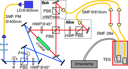
Figure 1: Schematic of the experimental setup, including the source of the non-maximally entangled photon pairs. A PPKTP crystal, cut and poled for type II spontaneous parametric down conversion from 405 nm to 810 nm, is placed at the waist of a Sagnac-style interferometer and pumped from both sides. Light at 810 nm from the two SPDC process is overlapped in a polarizing beam splitter (PBS), generating the non-maximally entangled state described by Eq. (4) when considering a single photon pair. A laser diode (LD) provides the continuous wave UV pump light. The combination of a half wave plate and polarization beam splitter (PBS) sets $\theta$ by controlling the relative intensity of the two pump beams, while a thin glass plate controls their relative phase $\phi$. The pump beams enter the interferometer through dichroic mirrors. At each output of the PBS, the combination of a HWP and PBS projects the mode polarization before coupling into a fiber single mode for light at 810 nm (SMF@810). A free space link is used to transfer light from SMF@810 to single mode fibers designed for 1550 nm (SMF-28e). Eventually the light is detected with high efficiency superconducting Transition Edge Sensors (TES), and timestamped with a resolution of 2 ns.

Experimental setup. – A sketch of the experimental setup is shown in Fig. 1. The source for entangled photon pairs is based on the coherent combination of two collinear type-II SPDC processes Fiorentino et al. (2004). We pump a periodically poled potassium titanylphyspate crystal (PPKTP, $2\times 1\times 10$ mm³) from two opposite directions with light from the same laser diode (405 nm). Both pump beams have the same Gaussian waists of $\approx 350\,\mu$m located within the crystal. Light at 810 nm from the two SPDC processes is overlapped in a polarizing beam splitter (PBS), entangling the polarization modes, and collected into single mode fibers. When a single photon pair is generated, the resulting polarization state is given by Eq. (4), where $\theta$ and $\phi$ are determined by the relative intensity and phase of the two pump beams set by rotating a half wave plate before the first PBS, and the tilt of a glass plate in one of the pump arms.

The effective collection modes for the downconverted light, determined by the single mode optical fibers and incoupling optics was chosen to have a Gaussian beam waist of $\approx 130~{}\mu$m centered in the crystal in order to maximize collection efficiency Bennink (2010); Ben Dixon et al. (2014). The combination of a zero-order half-wave plate and another PBS (extinction rate 1:1000 in transmission ) sets the measurement bases for light entering the single mode fibers. All optical elements are anti-reflection coated for 810 nm. Light from each collection fiber is sent to a superconducting transition edge sensor (TES) optimized for detection at 810 nm Lita et al. (2008), which are kept at $\approx 80$ mK within a cryostat. As the detectors show the highest efficiency when coupled to telecom fibers (SMF28+), the light collected in to single mode fibers from the parametric conversion source is transferred to these fibers via a free-space link. The TES output signal is translated into photodetection event arrival times using a constant fraction discriminator with an overall timing jitter $\approx 170$ ns, and recorded with a resolution of 2 ns. Setting Alice’s and Bob’s analyzing waveplates in the natural basis of the combining PBS, $HV$ and $VH$, we estimate heralded efficiencies of $82.42\pm 0.31$ % ($HV$) and $82.24\pm 0.30$ % ($VH$). We identified two main sources of uncorrelated detection events: intrinsic detector and background events at rates of $6.7\pm 0.58\,{\text{s}}^{-1}$ for Alice and $11.9\pm 0.77\,{\text{s}}^{-1}$ for Bob, respectively, and fluorescence caused by the UV pump in the PPKTP crystal Hegde et al. (2007), contributing $0.135\pm 0.08\%$ of the signal. With a total pump power at the crystal of 5.8 mW we estimate a pair generation rate $\approx 2.4\times 10^{4}\,{\text{s}}^{-1}$ (detected $\approx 20\times 10^{3}\,{\text{s}}^{-1}$), and dark count / background rates of 45.7 ${\text{s}}^{-1}$ (Alice) and 41.5 ${\text{s}}^{-1}$ (Bob).

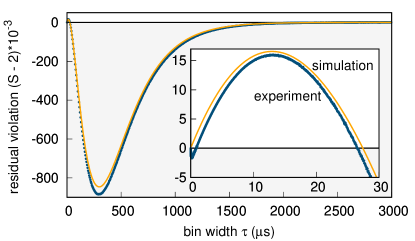
Figure 2: Measured CHSH violation as function of bin width $\tau$ (blue circles). A theoretical model (orange continuous line) is sketched in the main text and described in detail in Appendix A. Both the simulation and the experimental data show a violation for short $\tau$ (zoom in inset). The uncertainty on the measured value, calculated assuming i.i.d., corresponding to one standard deviation due to a Poissonian distribution of the events, is smaller than the symbols. For $\tau\lesssim 1~{}\mu$s the detection jitter ($\approx 170$ ns) is comparable with the time bin, resulting in a loss of observable correlation and a fast drop of the value of $S$.

Violation. – For the measured system efficiencies ($\eta_{A}\approx 82.4\%$, $\eta_{B}\approx 82.2\%$) and rate of uncorrelated counts at each detector (45.7 ${\text{s}}^{-1}$ Alice, 41.5 ${\text{s}}^{-1}$ Bob), a numerical optimisation gives the following values of the state and measurement parameters (see Appendix A for details): $\theta=25.9^{\circ}$, $\alpha_{0}=-7.2^{\circ}$, $\alpha_{1}=28.7^{\circ}$, $\beta_{0}=82.7^{\circ}$, and $\beta_{1}=-61.5^{\circ}$. These are close to optimal for all values of $\mu$, and the maximal violation is expected for $\mu=0.322$.

We collected data for approximately $42.8$ minutes, changing the measurement basis every 2 minutes, cycling through the four possible basis combinations. The sequence of the four settings is determined for every cycle using a pseudo-random number generator. We periodically ensure that $\phi\approx 0$ by rotating the phase plate until the visibility in the $+45^{\circ}/-45^{\circ}$ basis is larger than 0.985. Excluding the phase lock, the effective data acquisition time is $\approx 34$ min.

In Fig. 2 we show the result of processing the timestamped events for different bin widths $\tau$. The largest violation $S=2.01602(32)$ is observed for $\tau=13.150~{}\mu$s, which, with the cited pair generation rate of $24\times 10^{3}\,$s^-1, corresponds to $\mu\approx 0.32$. The uncertainty is calculated assuming that measurement results are independent and identically distributed (i.i.d.). Since the fluctuations of $S$ are identical in the i.i.d. and non-i.i.d. settings, this uncertainty is also representative of the p-value associated with local models Bierhorst (2015); Elkouss and Wehner (2016). The slight discrepancy between the experimental violation and the simulation is attributed to the non-ideal visibility of the state generated by the photon pair source. When $\tau$ is comparable to the detection jitter, detection events due to a single pair may be assigned to different rounds, decreasing the correlations. This explains the drop of $S$ below 2 (which our simulation does not capture because we have not included the jitter as a parameter).

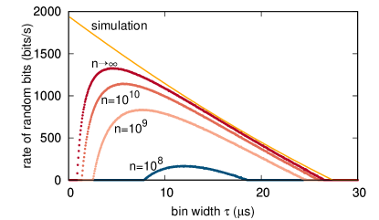
Figure 3: Randomness generation rate $r_{n}/\tau$ as a function of $\tau$ for different block sizes $n$. The points are calculated via Eq. (5) for finite $n$ (Eq. (6) for $n\to\infty$) and the violation measured in the experiment, assuming $\gamma=0$ (no testing rounds) and $\epsilon_{\textrm{c}}=\epsilon_{\textrm{s}}=10^{-10}$. The continuous line is the asymptotic rate Eq. (6) evaluated on the values of $S$ of the simulation shown in Fig. 2, for the same security assumptions.

Randomness extraction. – In order to turn the output data generated from our experiment into uniformly random bits, we need to employ a randomness expansion protocol Arnon-Friedman et al. (2018). Such a protocol consists of a pre-defined number of rounds $n$, forming a block. Each round is randomly assigned (with probability $\gamma$ and $1-\gamma$, respectively) to one of two tasks: testing the device for faults or eavesdropping attempts, or generating random bits. When the test rounds show a sufficient violation, one applies a quantum-proof randomness extractor to the block, obtaining $m$ random bits. The performance of the extraction protocol is determined by completeness and soundness security parameters, $\epsilon_{\textrm{c}}$ and $\epsilon_{\textrm{s}}$. To ensure the resulting string is uniform to within $\approx 10^{-10}$, we choose $\epsilon_{\textrm{c}}=\epsilon_{\textrm{s}}=10^{-10}$. The extraction protocol is a one-shot extraction protocol, i.e., the security analysis does not assume i.i.d.. The output randomness is composable and secure against a quantum adversary holding quantum side information Arnon-Friedman et al. (2018). The details of the protocol execution and its security proof are given in Appendix B.

For a block consisting of $n$ rounds, the number of random bits per round is at least

$$r_{n}=\eta_{\textrm{opt}}(\epsilon^{\prime},\epsilon_{\textrm{EA}})-4\frac{\log n}{n}+4\frac{\log\epsilon_{\textrm{EX}}}{n}-\frac{10}{n}\,,$$ (5)

where the function $\eta_{\textrm{opt}}$ depends on the block size $n$, detected violation $S$, and auxiliary security parameters $\epsilon^{\prime}$, $\epsilon_{\textrm{EA}}$, $\epsilon_{\textrm{EX}}$. The choice of these auxiliary security parameters is required to add up to the chosen level of completeness and soundness. In the limit $n\to\infty$ we obtain a lower bound on the number of random bits per round

$$r_{\infty}=\;1-h\left(\frac{1}{2}+\frac{1}{2}\sqrt{\frac{S^{2}}{4}-1}\right)\,,$$ (6)

where $h(p):=-p\,\log_{2}p-(1-p)\log_{2}(1-p)$ is the binary entropy function.

The extractable randomness rate $r_{n}/\tau$ based on the observed $S$ is presented in Fig. 3 for various block sizes $n$. For comparison, we also plot the asymptotic value $r_{\infty}/\tau$ with $S$ given by the simulation. The most obvious feature is that the highest randomness rate is not obtained at maximal violation of the inequality. There one gets highest randomness per round, but it turns out to be advantageous to sacrifice randomness per round in favor of a larger number of rounds per unit time. This optimization will be part of the calibration procedure for a random number generator with an active switch of measurement bases. As explained previously, the detection jitter affects the observable violation for $\tau$ comparable to it. This causes the sharp drop for short time bins observed for the experimental data. For fixed detector efficiencies, we expect the randomness rate to increase with higher photon pair generation rate, that is by increasing the pump power, and to be ultimately limited by the detection time jitter. Here, the use of efficient superconducting nanowire detectors will be a significant advantage.

We generated a random string from the data used to demonstrate the violation. We sacrificed $\approx 22$% of the data as calibration to determine the optimal bin width ($8.9~{}\mu$s), and estimate the corresponding violation. We applied the extractor to the remaining $\approx 78$% of the data, corresponding to 175 288 156 bins, obtaining 617 920 random bits. From the total measurement time of 42.8 min, we calculate a rate of $\approx 240$ random bit/s. For details of the extraction process see Appendix D. Considering only the net measurement time, that is without the acquisition of the calibration fraction of the data, the phase lock of the source, and the rotation of waveplate motors, we obtain a randomness rate of $\approx 396$ bit/s. These numbers are not necessarily optimal; more sophisticated analysis demonstrated randomness extraction for very low detected violations Bierhorst et al. (2018); Knill et al. (2017), and may yield a larger extractable randomness also in our case. Details of the extraction procedure are in Appendix D.

Conclusion. – We experimentally observed a violation of CHSH inequality with a continuous wave photon entangled pair source without the fair-sampling assumption combining a high collection efficiency source and high detection efficiency superconducting detectors, with the largest detected violation of $S=2.01602(32)$.

The generation rate of all probabilistic sources of entangled photon pairs is limited by the probability of generation of multiple pairs per experimental round, according to Poissonian statistics. The flexible definition of an experimental round permitted by the CW nature of our setup allowed us to study the dependence of the observable violation as function of the average number of photon pairs per experimental round. This same flexibility can be exploited to reduce the time necessary to acquire sufficient statistics for this kind of experiments: an increase in the pair generation rate is accompanied by a reduction of the round duration. This approach shifts the experimental repetition rate limitation from the photon statistics to the other elements of the setup, e.g. detectors time response or active polarization basis switching speed.

The observation of a Bell violation also certifies the generation of randomness. We estimate the amount of randomness generated per round both in an asymptotic regime and for a finite number of experimental rounds, assuming a required level of uniformity of $10^{-10}$. When considering the largest attainable rate of random bit generation, the optimal round duration is the result of the trade-off between observed violation and number of rounds per unit time. While for an ideal realization the optimal round duration would be infinitesimally short, it is limited in our system by the detection jitter time. Our proof of principle demonstration can be extended into a complete, loophole-free random number source. This requires closing the locality and freedom-of-choice loopholes, with techniques not different from pulsed photonic-sources, with the only addition of a periodic calibration necessary for determining the optimal time-bin.

Appendix A Modelling the violation of CHSH by a Poissonian source of qubit pairs

The output of a CW-pumped SPDC process can be accurately described as the emission of independent pairs distributed according to Poissonian statistics of average $\mu$, if the time under consideration (in our case, the length of a round) is much longer than the single-photon coherence time. The goal of this appendix is to provide an estimate of the observed CHSH parameter $S$ for such a source.

The pairs being independent, it helps to think in two steps. First, each pair is converted into classical information $(\alpha,\beta)\in\{+,-\}$ with probability

$$P_{Q}(\alpha,\beta|x,y)=\textrm{Tr}(\rho\Pi_{\alpha}^{x}\otimes\Pi_{\beta}^{y})\,,$$ (7)

where the $\Pi$’s are measurement operators. If some of the events have $\alpha=-$ ($\beta=-$), Alice’s (Bob’s) detector may be triggered, leading to the observed outcome $a=-1$ ($b=-1$).

For the purpose of studying CHSH, it is sufficient to consider $P(-1,+1|x,y)$ and $P(+1,-1|x,y)$, since

$$E_{xy}=1-P(-1,+1|x,y)-P(+1,-1|x,y)\,.$$ (8)

With our convention of outcomes, $P(-1,+1|x,y)$ is the probability associated with the case when Alice’s detector clicks and Bob’s does not. Thus, Bob’s detector should not be triggered by any pair: each pair will contribute to $P(-1,+1|x,y)$ with

$$D(\alpha)\equiv P_{Q}(\alpha,+|x,y)+(1-\eta_{B})P_{Q}(\alpha,-|x,y)\,.$$ (9)

Now, let us look at the contribution by $v$ pairs to $P(-1,+1|x,y)$. At least one of the $\alpha$’s must be $-$ for the detector to be triggered; and multiple detections will also be treated as $a=-1$. Thus, a configuration in which exactly $k$ $\alpha$’s are $-$ leads to $a=-1$ with probability $1-(1-\eta_{A})^{k}$ (i.e. at least one $\alpha=-$ must trigger a detection). Obviously there can be $\binom{v}{k}$ such configurations, so the contribution of the $v$ pair events to $P(-1,+1|x,y)$ is

$$D_{v}=\sum_{k=1}^{v}\binom{v}{k}[1-(1-\eta_{A})^{k}]D(-)^{k}D(+)^{v-k}\,.$$ (10)

Finally,

$$P(-1,+1|x,y)=\sum_{v=0}^{\infty}P_{\mu}(v)D_{v}\,.$$ (11)

The calculation of $P(+1,-1|x,y)$ is identical, with $D(\beta)\equiv P_{Q}(+,\beta|x,y)+(1-\eta_{A})P_{Q}(-,\beta|x,y)$ and $\eta_{B}$ instead of $\eta_{A}$ in (10).

Because the quantum probabilities appear in such a convoluted way, the optimal parameters for both the state and the measurements are not the same as for the single-pair case. Upon inspection, however, the values are close, as expected from the fact that the violation is mostly contributed by the single-pair events.

The curves presented in Fig. 2 have been obtained with a slightly modified model that includes the effect of the background events. The quantum probabilities $P_{Q}(\alpha,\beta|x,y)$ have been computed with $\rho=|{\psi}\rangle\langle{\psi}|$ given in (4) and with projective measurements, with the values of the parameters given in the main text.

Appendix B Protocol and security proof

For completeness, we will present the protocol studied in Arnon-Friedman et al. (2018) and give explicit constants in its security proof. We also refer to this paper for basic definitions of (smooth) min-entropy and related quantities. It will be more convenient for us to switch to to the notation $a,b\in\{0,1\}$ for the outcome labels (instead of $a,b\in\{+1,-1\}$ of the main text) and use the language of nonlocal games with winning condition

$$w_{\textrm{CHSH}}(a,b,x,y)=\begin{cases}1&\textrm{if }a\oplus b=x\cdot y\,,\\ 0&\textrm{otherwise}\,.\end{cases}$$ (12)

The game winning probability is then $w=1/2+S/8$ in terms of the CHSH value. The optimal classical winning strategy achieve a winning probability of 0.75, while the optimal quantum strategy achieves a winning probability of $(2+\sqrt{2})/4\approx 0.85$.

A randomness expansion protocol is a procedure that consumes $r$-bits of randomness and generates $m$-bits of almost uniform randomness. Formally, a $(\epsilon_{\textrm{c}},\epsilon_{\textrm{s}})$-secure $r\to m$ randomness expansion protocol if given $r$ uniformly random bits,

• (Soundness) For any implementation of the device it either aborts or returns an $m$-bit string $Z\in\{0,1\}^{m}$ with

  $$(1-\Pr[\textrm{abort}])\left\lVert\rho_{ZRE}-\rho_{U_{m}}\otimes\rho_{U_{r}}\otimes\rho_{E}\right\rVert_{1}\leq\epsilon_{\textrm{s}}\,,$$

  where $R$ is the input randomness register, $E$ is the adversary system, and $\rho_{U_{m}},\rho_{U_{r}}$ are the completely mixed states on appropriate registers.

• (Completeness) There exists an honest implementation with $\Pr[\textrm{abort}]\leq\epsilon_{\textrm{c}}$.

We remark that this security definition is a composable definition assuming quantum adversary, but not composable assuming a no-signalling adversary Arnon-Friedman et al. (2018). Composability allows the randomness generated to be safely used inside a larger protocol, such as quantum key distribution, without compromising the latter’s security.

For a concrete randomness expansion protocol, we present the protocol studied in Arnon-Friedman et al. (2018). The protocol takes parameters $\gamma$ expected fraction (marginal probability) of test rounds, $\omega_{\textrm{exp}}$ expected winning probability for an honest (perhaps noisy) implementation, and $\delta_{\textrm{est}}$ width of the statistical confidence interval for the estimation test. In an execution, for every round $i\in\{1,\dots,n\}$:

• Bob chooses a random bit $T_{i}\in\{0,1\}$ such that $\Pr(T_{i}=1)=\gamma$ using the interval algorithm Hao and Hoshi (1997).

• If $T_{i}=0$ (randomness generation), Alice and Bob choose deterministically $(X_{i},Y_{i})=(0,0)$, otherwise $T_{i}=1$ (test round) they choose uniformly random inputs $(X_{i},Y_{i})$.

• Alice and Bob use the physical devices with the said inputs $(X_{i},Y_{i})$ and record their outputs $(A_{i},B_{i})$.

• If $T_{i}=1$, they compute

  $$C_{i}=w_{\textrm{CHSH}}(A_{i},B_{i},X_{i},Y_{i})\,.$$ (13)

They abort the protocol if $\sum_{j}C_{j}<(\omega_{\textrm{exp}}\gamma-\delta_{\textrm{est}})n$ where $j$ is the index of test rounds, otherwise they return $\textrm{Ext}({\bf AB},{\bf Z})$ where Ext is a randomness extractor, ${\bf AB}=A_{1}B_{1}...A_{n}B_{n}$ and ${\bf Z}$ is a uniformly random seed.

More precisely, we use a Trevisan extractor in Mauerer et al. (2012) based on polynomial hashing with block weak design, because of its efficiency in terms of seed length. This is a function $\textrm{Ext}:\{0,1\}^{2n}\times\{0,1\}^{d}\to\{0,1\}^{m}$ such that if $H_{\textrm{min}}({\bf AB}|E)\geq 4\log\frac{1}{\epsilon_{1}}+6+m$ then

$$\frac{1}{2}\left\lVert\rho_{\textrm{Ext}({\bf AB},{\bf Z}){\bf Z}E}-\rho_{U_{m}}\otimes\rho_{U_{d}}\otimes\rho_{E}\right\rVert_{1}\leq m\epsilon_{1}$$ (14)

The seed length of this extractor is $d=a(2\ell)^{2}$ where

$$a =\left\lceil\frac{\log(m-2e)-\log(2\ell-2e)}{\log(2e)-\log(2e-1)}\right\rceil$$ (15)

$$\ell =\left\lceil\log 2n+2\log\frac{2}{\epsilon_{1}}\right\rceil$$ (16)

Now it can be shown that the entropy accumulation protocol gives the completeness and soundness of our randomness expansion protocol. However, let us mention how the input randomness affects the soundness and completeness of the final protocol.

In the protocol we assume access to a certain uniform randomness source, from which the random bits required in the protocol are generated: the $T_{i}$, $X_{i}$ and $Y_{i}$. In certain rounds, $X_{i}$ and $Y_{i}$ are either deterministic or fully random bits and can be directly obtained from the source. On the other hand, $T_{i}$ must be simulated from the uniform source (except when $\gamma=1/2$ which is not usually the case in practice). This can be done efficiently by the interval algorithm Hao and Hoshi (1997): the expected number of random bits needed to generate one Bernoulli$(\gamma)$ is at most $h(\gamma)+2$ and the maximum number of random bits needed is at most $L_{\max}:=\max\{\log\gamma^{-1},\log(1-\gamma)^{-1}\}$. Then Lemma 16 of Arnon-Friedman et al. (2018) gives us: let $\gamma>0$, for any $n$ there is an efficient procedure that given (at most) $6h(\gamma)n$ uniformly random bits either it aborts with probability at most $\epsilon_{\textrm{SA}}=\exp(-18h(\gamma)^{3}n/L_{\max})$ or outputs $n$ bits $T_{1},\dots,T_{n}$ whose distribution is within statistical distance at most $\epsilon_{\textrm{SA}}$ of $n$ i.i.d. Bernoulli$(\gamma)$ random variables. This raises both the completeness and soundness parameter of the final protocol by $\epsilon_{\textrm{SA}}$.

In an honest implementation of the protocol, Alice and Bob execute the protocol with a device that performs i.i.d. measurements on a tensor product state resulting in an expected winning probability $\omega_{\textrm{exp}}$. Here Lemma 8 of Arnon-Friedman et al. (2018) bounds the probability of aborting using Hoeffding’s inequality. That is, the probability that our randomness expansion protocol aborts for an honest implementation is

$$\Pr[\textrm{abort}]\leq\exp(-2n\delta_{\textrm{est}}^{2})=:\epsilon_{\textrm{est}}\,.$$ (17)

Therefore, the total completeness is bounded by $\epsilon_{\textrm{SA}}+\epsilon_{\textrm{est}}$. (Note that $\epsilon_{\textrm{est}}$ is actually the completeness parameter of the entropy accumulation protocol in Arnon-Friedman et al. (2018).)

For the soundness, Corollary 11 of Arnon-Friedman et al. (2018) ensures that for any $\epsilon_{\textrm{EA}},\epsilon^{\prime}\in(0,1)$ either the protocol aborts with probability greater than $1-\epsilon_{\textrm{EA}}$ or

$$H_{\textrm{min}}^{\epsilon^{\prime}}({\bf AB}|{\bf XYT}E)_{\rho_{|\textrm{pass}}}>n\cdot\eta_{\textrm{opt}}(\epsilon^{\prime},\epsilon_{\textrm{EA}})\,.$$ (18)

Together with our extractor, for all $\epsilon_{1}\in(0,1)$, if the length $m$ of the final string satisfies

$$n\cdot\eta_{\textrm{opt}}(\epsilon^{\prime},\epsilon_{\textrm{EA}})=4\log\frac{1}{\epsilon_{1}}+6+m$$ (19)

then we are guaranteed that

$$\frac{1}{2}\left\lVert\rho_{SRE}-\rho_{U_{m}}\otimes\rho_{U_{R}}\otimes\rho_{E}\right\rVert_{1}\leq\epsilon^{\prime}/2+m\epsilon_{1}\,.$$ (20)

Here $\eta_{\textrm{opt}}(\epsilon^{\prime},\epsilon_{\textrm{EA}})$ is given by the following equations: for $h$ the binary entropy and $\gamma,p(1)\in(0,1]$

$$\eta_{\textrm{opt}}(\epsilon^{\prime},\epsilon_{\textrm{EA}}) =\max_{\frac{3}{4}<\frac{p_{t}(1)}{\gamma}<\frac{2+\sqrt{2}}{4}}\eta(\omega_{\textrm{exp}}\gamma-\delta_{\textrm{est}},p_{t},\epsilon^{\prime},\epsilon_{\textrm{EA}})\,,$$ (21)

$$\eta(p,p_{t},\epsilon^{\prime},\epsilon_{\textrm{EA}}) =f_{\min}(p,p_{t})-\frac{1}{\sqrt{n}}2\left(\log 13+\frac{\mathrm{d}}{\mathrm{d}p(1)}g(p)|_{p_{t}}\right)\sqrt{1-2\log(\epsilon^{\prime}\epsilon_{\textrm{EA}})}\,,$$ (22)

$$f_{\min}(p,p_{t}) =\begin{cases}g(p)&\textrm{ if }p(1)\leq p_{t}(1)\,,\\ \frac{\mathrm{d}}{\mathrm{d}p(1)}g(p)|_{p_{t}}\cdot p(1)+\left(g(p_{t})-\frac{\mathrm{d}}{\mathrm{d}p(1)}g(p)|_{p_{t}}\cdot p_{t}(1)\right)&\textrm{ if }p(1)>p_{t}(1)\end{cases}$$ (23)

$$g(p) =\begin{cases}1-h\left(\frac{1}{2}+\frac{1}{2}\sqrt{16\frac{p(1)}{\gamma}\left(\frac{p(1)}{\gamma}-1\right)+3}\right)&\textrm{ if }\frac{p(1)}{\gamma}\in\left[0,\frac{2+\sqrt{2}}{4}\right]\\ 1&\textrm{ if }\frac{p(1)}{\gamma}\in\left[\frac{2+\sqrt{2}}{4},1\right]\end{cases}$$ (24)

Combined with the input sampling soundness, the total soundness is bounded by $\epsilon_{\textrm{SA}}+\epsilon_{\textrm{EA}}+\epsilon^{\prime}/2+m\epsilon_{1}$.

Parameter	Definition
$\epsilon_{\textrm{c}}$	completeness, bounding honest abort probability
$\epsilon_{\textrm{s}}$	soundness, bounding randomness security
$\epsilon_{\textrm{SA}}$	input sampling error tolerance
$\epsilon^{\prime}$	smoothing parameter
$\epsilon_{1}$	1-bit extractor error tolerance
$\epsilon_{\textrm{EX}}$	randomness extractor error tolerance
$\epsilon_{\textrm{est}}$	Bell estimation error tolerance
$\epsilon_{\textrm{EA}}$	soundness of entropy accumulation protocol

Table 1: Definition of security parameters.

Finally, let us count the number of random bits consumed in the protocol. It consists of the randomness used to decide if a round is a test or generation round, the randomness used to pick the inputs in a test round, and the randomness used for the Trevisan extractor. Taking into account the finite statistical fluctuations, we need at most $6h(\gamma)n$ bits to choose between test and generation except with probability $\epsilon_{\textrm{SA}}$. This results in at most $2\gamma n$ testing rounds except with probability $\epsilon_{\textrm{SA}}$, which equates to $2\times 2\gamma n$ random bits being consumed for generating the inputs for test rounds. The randomness for Trevisan extractor is $d$ bits. (Practically, after the first run of the protocol, we can omit this amount because the extractor is a strong extractor: we can reuse the seed for next run of the protocol). Summing these up, we have consumed at most $6h(\gamma)n+4\gamma n+d$ uniformly random bits with probability at least $1-2\epsilon_{\textrm{SA}}$.

In summary, for a device with $\omega_{\textrm{exp}}$, any choice of $\gamma,\epsilon_{1},\epsilon^{\prime},\epsilon_{\textrm{EA}}\in(0,1)$, and $n$ large enough, our protocol is an $(\epsilon_{\textrm{SA}}+\epsilon_{\textrm{est}},\epsilon_{\textrm{SA}}+\epsilon_{\textrm{EA}}+\epsilon^{\prime}/2+m\epsilon_{1})$-secure $[6h(\gamma)n+4\gamma n+d]\to m$ randomness expansion protocol. That is either our protocol abort with probability greater than $1-\epsilon_{\textrm{EA}}$, or it produces a string of length $m$ such that $\frac{1}{2}\left\lVert\rho_{SRE}-\rho_{U_{m}}\otimes\rho_{U_{R}}\otimes\rho_{E}\right\rVert\leq\epsilon_{\textrm{SA}}+\epsilon^{\prime}/2+m\epsilon_{1}$ . The protocol consume at most $6h(\gamma)n+4\gamma n+d$ uniformly random bits with probability at least $1-2\epsilon_{\textrm{SA}}$.

Appendix C Input/Output randomness analysis

The previous Appendix gives a complete picture of the (one-shot) behavior of our randomness expansion protocol. For the purpose of this paper, it suffices to obtain rough estimates on the randomness output, but further optimization can be done.

For simplicity, we introduce some bounds on the resources. Since $m\leq 2n$ we can let $m\epsilon_{1}\leq 2n\epsilon_{1}=:\epsilon_{\textrm{EX}}$ which gives $\epsilon_{1}=\epsilon_{\textrm{EX}}/(2n)$. Plugging this back in (19) gives us the number of random bits one can extract,

$$m=n\cdot\eta_{\textrm{opt}}(\epsilon^{\prime},\epsilon_{\textrm{EA}})-4\log n+4\log\epsilon_{\textrm{EX}}-10\,,$$ (25)

for a given level of soundness $\epsilon_{\textrm{SA}}+\epsilon_{\textrm{EA}}+\epsilon^{\prime}/2+\epsilon_{\textrm{EX}}$. Moreover, the protocol consumes $6h(\gamma)n+4\gamma n+d$ bits of randomness with probability at least $1-\epsilon_{\textrm{SA}}$, where

$$d=a(2\ell)^{2} \textrm{ with }a\leq\frac{\log(2n-2e)-\log(2\ell-2e)}{\log(2e)-\log(2e-1)}+1$$

$$\textrm{ and }\,\,\,\ell\leq 3\log n+6-2\log\epsilon_{\textrm{EX}}\,.$$ (26)

This leads to an expansion of $m-6h(\gamma)n-4\gamma n-d$. Hence, the output randomness rate per unit time is

$$r_{n}=\frac{1}{\tau}\left(\eta_{\textrm{opt}}(\epsilon^{\prime},\epsilon_{\textrm{EA}})-4\frac{\log n}{n}+4\frac{\log\epsilon_{\textrm{EX}}}{n}-\frac{10}{n}\right)\,,$$ (27)

and the net randomness rate per unit time is

$$r^{\textrm{net}}_{n}=\frac{1}{\tau}\left(\eta_{\textrm{opt}}(\epsilon^{\prime},\epsilon_{\textrm{EA}})-4\frac{\log n}{n}+4\frac{\log\epsilon_{\textrm{EX}}}{n}-\frac{10}{n}-6h(\gamma)-4\gamma-\frac{d}{n}\right)\,.$$ (28)

These formulas are of course given for a protocol with completeness $\epsilon_{\textrm{SA}}+\epsilon_{\textrm{est}}$ and soundness $\epsilon_{\textrm{SA}}+\epsilon_{\textrm{EA}}+\epsilon^{\prime}/2+\epsilon_{\textrm{EX}}$, where

$$\epsilon_{\textrm{SA}} =\exp(-18h(\gamma)^{3}n/L_{\max})$$ (29)

$$L_{\max} =\max\{\log\gamma^{-1},\log(1-\gamma)^{-1}\}$$ (30)

$$\epsilon_{\textrm{est}} =\exp(-2n\delta_{\textrm{est}}^{2})\,.$$ (31)

The asymptotic rate for the block size $n\to\infty$ is given by taking the limit of block size $n$

$$r_{\infty}=\frac{1}{\tau}\;\left[1-h\left(\frac{1}{2}+\frac{1}{2}\sqrt{\frac{S^{2}}{4}-1}\right)\right]\,.$$ (32)

For the net asymptotic rate we could also take the same limit, however we could obtain a better bound by the expected behavior of the interval algorithm. Since the expected number of random bits needed to generate $T_{1},...,T_{n}$ is $nh(\gamma)+2$ by Hao and Hoshi (1997), and $\gamma n$ of which is expected to be test rounds each consuming 2 random bits, we have the asymptotic net rate

$$r_{\infty}^{\textrm{net}}=\frac{1}{\tau}\;\left[1-h\left(\frac{1}{2}+\frac{1}{2}\sqrt{\frac{S^{2}}{4}-1}\right)-h(\gamma)-2\gamma\right]\,.$$ (33)

From an end-user perspective, one may argue that the only parameters of interest are the completeness and soundness security parameters which will constrain the rest of protocol parameters—$\gamma,\delta_{\textrm{est}},n,\epsilon$’s—for a given objective such as maximizing randomness rate or net randomness rate. For the illustrative plots we set the constraints

$$\epsilon_{\textrm{SA}}+\epsilon_{\textrm{EA}}+\epsilon^{\prime}/2+\epsilon_{\textrm{EX}} =\epsilon_{\textrm{s}}\,,$$ (34)

$$\epsilon_{\textrm{SA}}+\epsilon_{\textrm{est}} =\epsilon_{\textrm{c}}\,,$$ (35)

and fix $\epsilon_{\textrm{c}}=10^{-10},\epsilon_{\textrm{s}}=10^{-10}$. One then maximizes randomness output or net randomness output given these constraints. This gives us the best (as measured by our objective function) protocol parameters within the relaxations made to obtain (25) and (26).

However, in the main text we take a simpler approach without optimizing over the variables $\gamma,\delta_{\textrm{est}},\epsilon$’s. For each block size $n$, we compute $\epsilon_{\textrm{SA}}$ as given by (29) which then fixes $\delta_{\textrm{est}}$ via $\epsilon_{\textrm{est}}=10^{-10}-\epsilon_{\textrm{SA}}$ and (31). The remaining $\epsilon$’s which have weight $10^{-10}-\epsilon_{\textrm{SA}}$ are chosen in a $1:2:1$ ratio of $\epsilon_{\textrm{EA}}:\epsilon^{\prime}:\epsilon_{\textrm{EX}}$, which is guaranteed to add up to the specified level of completeness and soundness. This approach is not far from optimal in the regime of large block size $n$. This results in the experimental points reported in Figure 3.

Appendix D Random bits extraction procedure

As mentioned in the main text, the data observed during the experiment contains certified randomness. Here we describe the procedure we use to extract this randomness in a finite run of the experiment. We consider two blocks of data, corresponding to an acquisition time of $\approx 42.8$ min (dataset1) and $\approx 17.33$ hours (dataset2).

The randomness protocol we use (described in Appendix B) relies on two elements:

• an honest implementation, and

• security parameters.

These elements must be chosen adequately before proceeding to the extraction. Indeed, if a too optimistic honest implementation is chosen, for instance, the data observed will fail to pass the test, and the whole protocol will abort: no randomness can then be extracted.

Moreover, our setup allows us to choose freely the

• bin width

which can significantly affect the amount of certified randomness.

We dedicate a fraction $\gamma_{\text{calib}}$ of our data to the estimation of these parameters so as to maximize the amount of randomness certified. The randomness protocol is then run with these parameters on the remaining fraction $(1-\gamma_{\text{calib}})$ of the data only. We determine the fraction of data $\gamma_{\text{calib}}$ to use for the calibration of the randomness extraction procedure from a simulation of the experiment. We estimate the number of random bits that can be certified from an experiment of the envisioned length if a fraction $\gamma_{\text{calib}}$ of the data is dedicated to calibration purpose (all other parameters being set as expected). We choose the value of $\gamma_{\text{calib}}$ that maximizes this quantity. We find that $\gamma_{\text{calib}}=22\%$ is adequate for dataset1, and $\gamma_{\text{calib}}=8\%$ for dataset2.

We then proceed to define the parameters of the randomness protocol. The security parameters $\epsilon_{\textrm{s}},\epsilon_{\textrm{c}}$ are set a priori, with all the other parameters derived as described in Appendices B and C, with $\gamma=1$. We define honest implementation an implementation which reproduces the CHSH violation observed during the calibration stage with probability

$$P(S_{\text{exp}}\geq S_{\text{calib}})\geq\epsilon_{\text{calib}}\,.$$ (36)

For concreteness, we set $\epsilon_{\text{calib}}=10^{-10}$. This step guarantees that we will not overestimate the amount of Bell violation which we can expect from a honest experiment. This is crucial for the whole certification procedure to succeed with a large probability. We then have

$$w_{\text{exp}}=w_{\text{calib}}-\delta_{\text{calib}}\,,$$ (37)

with $\delta_{\text{calib}}=B(\omega_{\text{exp}},(1-\gamma_{\text{calib}})n,\omega_{\text{calib}})$, where

$$B(p,n,q)=\sum_{i=0}^{nq}\binom{n}{i}p^{i}(1-p)^{n-i}$$ (38)

is the cumulative distribution of $n$ Bernoulli variable with parameter $p$. For simplicity, we use the upper bound

$$\delta_{\text{calib}}\leq\sqrt{\frac{\log(1/\epsilon_{\text{calib}})}{2n}}$$ (39)

valid for all winning probability $\omega_{\text{calib}}$, which leads to a conservative estimate of the honest implementation Bell violation $S_{\text{est}}$.

Having fixed all security parameters and defined our honest implementation, we are now left with the choice of the bin width. For this, following the procedure discussed in the main text, we compute the number of certified random bits that we can hope to certify in the remaining $(1-\gamma_{\text{calib}})$ fraction of the data as a function of the bin width. We then choose the bin width which yields the maximum rate of random bits. We find that optimal bin widths 8.9 $\mu$s for dataset1 and 5.35 $\mu$s for dataset2. This allows us to define how the remaining data is to be treated: first, we extract the outcomes corresponding to the chosen bin width, then we use the exact number of bins so extracted to compute precisely the threshold Bell violation $w_{\text{exp}}-\delta_{\text{est}}$ and the number of certified bits $m$ corresponding to this dataset, finally we check whether the data indeed yields a Bell violation larger than $w_{\text{exp}}-\delta_{\text{est}}$. If this is not the case, we abort. Otherwise, we apply a randomness extractor on the string of outcomes. Both datasets pass this test.

Finally, we use the Trevisan extractor implemented by Mauerer et al. Mauerer et al. (2012), and further improved by Bierhorst et al. Bierhorst et al. (2018) to extract the certified bits. The advantage of Trevisan extractors over other kinds of randomness extractors is that they require little initial seeds, and that they are composable, strong extractors, and secure against quantum side information. Following the suggestion of Mauerer et al. (2012), we use the block weak design construction with a RSH extractor to maximize the number of extracted bits. The extractor also require a supply of seed randomness. For this, we use the bits generated with the random number generator described in Shi et al. (2016).

In the end, we extract 617 920 and 35 799 872 uniformly random bits from dataset1 and dataset2 respectively, using seeds of length 1 808 802 and 2 923 224. The corresponding rates, calculated including the acquisition time of the calibration data, source phase lock and basis switching, are $\approx 240$ bits/s and $\approx~{}573$ bits/s. If we consider only the time necessary for the data acquisition, we obtain net randomness rates of $\approx 396$ bit/s and $\approx 943$ bit/s.

These rates do not include the processing time of the Trevisan extractor. This classical computation took 9 hours for dataset1 and 22 days for dataset2 on a machine processing 24 threads in parallel. This task could be heavily parallelized. The bits extracted can be found in the ancillary files anc .

We used the NIST Statistical Test Suite Rukhin et al. (2010) to ensure the quality of generated strings is at least on par with acceptable pseudo-randomness. This suit of test can only verify the uniformity of the generated random string, it does not certify its privacy. The string generated from dataset1 passed all the tests that are meaningful for this relatively short data sample, assuming an acceptable significance level $\alpha=0.01$. The result of the individual tests are summarized in table 2.

Test	$P$–value	Proportion
Frequency	0.590949	96/97
Block Frequency	0.275709	95/97
Cumulative Sums Forward	0.964295	96/97
Cumulative Sums Backward	0.637119	96/97
Runs	0.162606	97/97
Longest Run of Ones	0.590949	96/97
Discrete Fourier Transform	0.183769	96/97

Table 2: Result of the NIST Statistical Test Suite for the bits extracted from dataset1. We split the random bits into 97 sequences of 6300 bits each.

References

- Colbeck (2007) R. Colbeck, Quantum And Relativistic Protocols For Secure Multi-Party Computation, Ph.D. thesis, University of Cambridge (2007).
- Pironio et al. (2010) S. Pironio, A. Acín, S. Massar, A. B. de la Giroday, D. N. Matsukevich, P. Maunz, S. Olmschenk, D. Hayes, L. Luo, T. A. Manning, and C. R. Monroe, Nature 464, 1021 (2010).
- Acín and Masanes (2016) A. Acín and L. Masanes, Nature 540, 213 (2016).
- Hensen et al. (2015) B. J. Hensen, H. Bernien, A. E. Dréau, A. Reiserer, N. Kalb, M. S. Blok, J. Ruitenberg, R. F. L. Vermeulen, R. N. Schouten, C. Abellán, W. Amaya, V. Pruneri, M. W. Mitchell, M. Markham, D. J. Twitchen, D. Elkouss, S. Wehner, T. H. Taminiau, and R. Hanson, Nature 526, 682 (2015).
- Lita et al. (2008) A. E. Lita, A. J. Miller, and S. W. Nam, Opt. Express 16, 3032 (2008).
- Marsili et al. (2013) F. Marsili, V. B. Verma, J. A. Stern, S. Harrington, A. E. Lita, T. Gerrits, I. Vayshenker, B. Baek, M. D. Shaw, R. P. Mirin, and S. W. Nam, Nature Photonics 7, 210 (2013).
- Giustina et al. (2015) M. Giustina, M. A. M. Versteegh, S. Wengerowsky, J. Handsteiner, A. Hochrainer, K. Phelan, F. Steinlechner, J. Kofler, J.-A. Larsson, C. Abellán, W. Amaya, V. Pruneri, M. W. Mitchell, J. Beyer, T. Gerrits, A. E. Lita, L. K. Shalm, S. W. Nam, T. Scheidl, R. Ursin, B. Wittmann, and A. Zeilinger, Phys. Rev. Lett. 115, 250401 (2015).
- Shalm et al. (2015) L. K. Shalm, E. Meyer-Scott, B. G. Christensen, and P. Bierhorst, Phys. Rev. 115, 250402 (2015).
- Bierhorst et al. (2018) P. Bierhorst, E. Knill, S. Glancy, Y. Zhang, A. Mink, S. Jordan, A. Rommal, Y.-K. Liu, B. Christensen, S. W. Nam, M. J. Stevens, and L. K. Shalm, Nature 556, 223 (2018).
- Liu et al. (2018) Y. Liu, X. Yuan, M.-H. Li, W. Zhang, Q. Zhao, J. Zhong, Y. Cao, Y.-H. Li, L.-K. Chen, H. Li, T. Peng, Y.-A. Chen, C.-Z. Peng, S.-C. Shi, Z. Wang, L. You, X. Ma, J. Fan, Q. Zhang, and J.-W. Pan, Phys. Rev. Lett. 120, 010503 (2018).
- Larsson and Gill (2004) J.-A. Larsson and R. D. Gill, EPL 67, 707 (2004).
- Christensen et al. (2015) B. G. Christensen, A. Hill, E. Knill, S. W. Nam, K. J. Coakley, S. Glancy, L. K. Shalm, and Y. Zhang, Phys. Rev. A 92, 032130 (2015).
- Giustina et al. (2013) M. Giustina, A. Mech, S. Ramelow, B. Wittmann, J. Kofler, J. Beyer, A. E. Lita, B. Calkins, T. Gerrits, S. W. Nam, R. Ursin, and A. Zeilinger, Nature 497, 227 (2013).
- Bancal et al. (2014) J.-D. Bancal, L. Sheridan, and V. Scarani, New J. Phys. 16, 033011 (2014).
- Eberhard (1993) P. H. Eberhard, Phys. Rev. A 47, R747 (1993).
- Caprara Vivoli et al. (2015) V. Caprara Vivoli, P. Sekatski, J.-D. Bancal, C. C. W. Lim, B. G. Christensen, A. Martin, R. T. Thew, H. Zbinden, N. Gisin, and N. Sangouard, Phys. Rev. A 91, 012107 (2015).
- Fiorentino et al. (2004) M. Fiorentino, G. Messin, C. E. Kuklewicz, F. N. C. Wong, and J. H. Shapiro, Phys. Rev. A 69, 041801 (2004).
- Bennink (2010) R. S. Bennink, Phys. Rev. A 81, 053805 (2010).
- Ben Dixon et al. (2014) P. Ben Dixon, D. Rosenberg, V. Stelmakh, M. E. Grein, R. S. Bennink, E. A. Dauler, A. J. Kerman, R. J. Molnar, and F. N. C. Wong, Phys. Rev. A 90, 043804 (2014).
- Hegde et al. (2007) S. M. Hegde, K. L. Schepler, R. D. Peterson, and D. E. Zelmon, in Defense and Security Symposium, edited by G. L. Wood and M. A. Dubinskii (SPIE, 2007) p. 65520V.
- Bierhorst (2015) P. Bierhorst, J. Phys. A: Math. Theor. 48, 195302 (2015).
- Elkouss and Wehner (2016) D. Elkouss and S. Wehner, npj Quantum Inf 2, 042111 (2016).
- Arnon-Friedman et al. (2018) R. Arnon-Friedman, F. Dupuis, O. Fawzi, R. Renner, and T. Vidick, Nat Comms 9, 459 (2018).
- Knill et al. (2017) E. Knill, Y. Zhang, and P. Bierhorst, ArXiv e-prints (2017), arXiv:1709.06159 [quant-ph] .
- Hao and Hoshi (1997) T. S. Hao and M. Hoshi, IEEE Transactions on Information Theory 43, 599 (1997).
- Mauerer et al. (2012) W. Mauerer, C. Portmann, and V. B. Scholz, ArXiv e-prints (2012), arXiv:1212.0520 .
- Shi et al. (2016) Y. Shi, B. Chng, and C. Kurtsiefer, Appl. Phys. Lett. 109, 041101 (2016).
- (28) https://arxiv.org/help/ancillary_files.
- Rukhin et al. (2010) A. Rukhin, J. Soto, J. Nechvatal, M. Smid, E. Barker, S. Leigh, M. Levenson, M. Vangel, D. Banks, A. Heckert, J. Dray, and S. Vo, “A statistical test suite for the validation of cryptographic random number generators,” National Institute of Standards and Technology, Gaithersburg (2010).