Hierarchical Structured Model for Fine-to-coarse Manifesto Text Analysis

Abstract

Election manifestos document the intentions, motives, and views of political parties. They are often used for analysing a party’s fine-grained position on a particular issue, as well as for coarse-grained positioning of a party on the left–right spectrum. In this paper we propose a two-stage model for automatically performing both levels of analysis over manifestos. In the first step we employ a hierarchical multi-task structured deep model to predict fine- and coarse-grained positions, and in the second step we perform post-hoc calibration of coarse-grained positions using probabilistic soft logic. We empirically show that the proposed model outperforms state-of-art approaches at both granularities using manifestos from twelve countries, written in ten different languages.

1 Introduction

The adoption of NLP methods has led to significant advances in the field of computational social science Lazer et al. (2009), including political science Grimmer and Stewart (2013). Among a myriad of data sources, election manifestos are a core artifact in political analysis. One of the most widely used datasets by political scientists is the Comparative Manifesto Project (CMP) dataset Volkens et al. (2017), which contains manifestos in various languages, covering over 1000 parties across 50 countries, from elections dating back to 1945.

In CMP, a subset of the manifestos has been manually annotated at the sentence-level with one of 57 political themes, divided into 7 major categories. Such categories capture party positions (favorable, unfavorable or neither) on fine-grained policy themes, and are also useful for downstream tasks including calculating manifesto-level (policy-based) left–right position scores Budge et al. (2001); Lowe et al. (2011); Däubler and Benoit (2017). An example sentence from the Green Party of England and Wales 2015 election manifesto where they take an unfavorable position on military is:

We would: Ensure that … less is spent on military research.

Elsewhere, they take a favorable position on welfare state:

Double Child Benefit.

Such manual annotations are labor-intensive and prone to annotation inconsistencies Mikhaylov et al. (2012). In order to overcome these challenges, supervised sentence classification approaches have been proposed Verberne et al. (2014); Subramanian et al. (2017).

Other than the sentence-level labels, the manifesto text also has a document-level score that quantifies its position on the left–right spectrum. Different approaches have been proposed to derive this score, based on alternate definitions of “left–right” Slapin and Proksch (2008); Benoit and Laver (2007); Lo et al. (2013); Däubler and Benoit (2017). Among these, the RILE index is the most widely adopted Merz et al. (2016); Jou and Dalton (2017), and has been shown to correlate highly with other popular scores Lowe et al. (2011). RILE is defined as the difference between right and left positions on (pre-determined) policy themes across sentences in a manifesto Volkens et al. (2013); for instance, unfavorable position on military is categorized as left. RILE is popular in CMP in particular, as mapping individual sentences to left/right/neutral categories has been shown to be less sensitive to systematic errors than other sentence-level class sets Klingemann et al. (2006); Volkens et al. (2013).

Finally, expert survey scores are gaining popularity as a means of capturing manifesto-level political positions, and are considered to be context- and time-specific, unlike RILE Volkens et al. (2013); Däubler and Benoit (2017). We use the Chapel Hill Expert Survey (CHES) Bakker et al. (2015), which comprises aggregated expert surveys on the ideological position of various political parties. Although CHES is more subjective than RILE, the CHES scores are considered to be the gold-standard in the political science domain.

In this work, we address both fine- and coarse-grained multilingual manifesto text policy position analysis, through joint modeling of sentence-level classification and document-level positioning (or ranking) tasks. We employ a two-level structured model, in which the first level captures the structure within a manifesto, and the second level captures context and temporal dependencies across manifestos. Our contributions are as follows:

• we employ a hierarchical sequential deep model that encodes the structure in manifesto text for the sentence classification task;

• we capture the dependency between the sentence- and document-level tasks, and also utilize additional label structure (categorization into left/right/neutral: Volkens et al. (2013)) using a joint-structured model;

• we incorporate contextual information (such as political coalitions) and encode temporal dependencies to calibrate the coarse-level manifesto position using probabilistic soft logic Bach et al. (2015), which we evaluate on the prediction of the RILE index or expert survey party position score.

2 Related Work

Analysing manifesto text is a relatively new application at the intersection of political science and NLP. One line of work in this space has been on sentence-level classification, including classifying each sentence according to its major political theme (1-of-7 categories) Zirn et al. (2016); Glavaš et al. (2017a), its position on various policy themes Verberne et al. (2014); Biessmann (2016); Subramanian et al. (2017), or its relative disagreement with other parties Menini et al. (2017). Recent approaches Glavaš et al. (2017a); Subramanian et al. (2017) have also handled multilingual manifesto text (given that manifestos span multiple countries and languages; see Section 5.1) using multilingual word embeddings.

At the document level, there has been work on using label count aggregation of (manually-annotated) fine-grained policy positions, as features for inductive analysis Lowe et al. (2011); Däubler and Benoit (2017). Text-based approaches has used dictionary-based supervised methods, unsupervised factor analysis based techniques and graph propagation based approaches Hjorth et al. (2015); Bruinsma and Gemenis (2017); Glavaš et al. (2017b). A recent paper closely aligned with our work is Subramanian et al. (2017), who address both sentence- and document-level tasks jointly in a multilingual setting, showing that a joint approach outperforms previous approaches. But they do not exploit the structure of the text and use a much simpler model architecture: averages of word embeddings, versus our bi-LSTM encodings; and they do not leverage domain information and temporal regularities that can influence policy positions Greene (2016). This work will act as a baseline in our experiments in Section 5.

Policy-specific position classification can be seen as related to target-specific stance classification Mohammad et al. (2017), except that the target is not explicitly mentioned in most cases. Secondly, manifestos have both fine- and coarse-grained positions, similar to sentiment analysis McDonald et al. (2007). Finally, manifesto text is well structured within and across documents (based on coalition), has temporal dependencies, and is multilingual in nature.

3 Proposed Approach

In this section, we detail the first step of our two-stage approach. We use a hierarchical bidirectional long short-term memory (“bi-LSTM”) model Hochreiter and Schmidhuber (1997); Graves et al. (2013); Li et al. (2015) with a multi-task objective for the sentence classification and document-level regression tasks. A post-hoc calibration of coarse-grained manifesto position is given in Section 4.

Let $D$ be the set of manifestos, where a manifesto $d\in D$ is made up of $L$ sentences, and a sentence $s_{i}$ has $T$ words: $w_{i1},w_{i2},...w_{iT}$. The set $D_{s}\subset D$ is annotated at the sentence-level with positions on fine-grained policy issues (57 classes). The task here is to learn a model that can: (a) classify sentences according to policy issue classes; and (b) score the overall document on the policy-based left–right spectrum (RILE), in an inter-dependent fashion.

Word encoder: We initialize word vector representations using a multilingual word embedding matrix, $W_{e}$. We construct $W_{e}$ by aligning the embedding matrices of all the languages to English, in a pair-wise fashion. Bilingual projection matrices are built using pre-trained FastText monolingual embeddings Bojanowski et al. (2017) and a dictionary $D$ constructed by translating 5000 frequent English words using Google Translate. Given a pair of embedding matrices $E$ (English) and $O$ (Other), we use singular value decomposition of $O^{T}DE$ (which is $U\Sigma V^{T}$) to get the projection matrix ($W^{*}$=$UV^{T}$), since it also enforces monolingual invariance Artetxe et al. (2016); Smith et al. (2017). Finally, we obtain the aligned embedding matrix, $W_{e}$, as $OW^{*}$.

We use a bi-LSTM to derive a vector representation of each word in context. The bi-LSTM traverses the sentence $s_{i}$ in both the forward and backward directions, and the encoded representation for a given word $\mathbf{w}_{it}\in s_{i}$, is defined by concatenating its forward ($\overrightarrow{\mathbf{h}}_{it}$) and backward hidden states ($\overleftarrow{\mathbf{h}}_{it}$), $t\in\big{[}1,T\big{]}$.

Sentence model: Similarly, we use a bi-LSTM to generate a sentence embedding from the word-level bi-LSTM, where each input sentence $s_{i}$ is represented using the last hidden state of both the forward and backward LSTMs. The sentence embedding is obtained by concatenating the hidden representations of the sentence-level bi-LSTM, in both the directions, $\mathbf{h}_{i}$ = [$\overrightarrow{\mathbf{h}}_{i}$, $\overleftarrow{\mathbf{h}}_{i}$], i $\in\big{[}1,L\big{]}$. With this representation, we perform fine-grained classification (to one-of-57 classes), using a softmax output layer for each sentence. We minimize the cross-entropy loss for this task, over the sentence-level labeled set $D_{s}\subset D$. This loss is denoted $\mathcal{L}_{S}$.

Document model: To represent a document $d$ we use average-pooling over the sentence representations $\mathbf{h}_{i}$ and predicted output distributions ($\mathbf{y}_{i}$) of individual sentences, i.e., $\mathbf{V}_{d}=\frac{1}{L}\sum_{i\in d}\left[\begin{array}[]{cc}\mathbf{y}_{i}\\ \mathbf{h}_{i}\end{array}\right]$. The range of RILE is $[-100,100]$, which we scale to the range $[-1,1]$, and model using a final $\tanh$ layer. We minimize the mean-squared error loss function between the predicted $\hat{r}_{d}$ and actual RILE score $r_{d}$, which is denoted as $\mathcal{L}_{D}$:

$$\mathcal{L}_{D}=\frac{1}{|D|}\sum_{d=1}^{|D|}\|\hat{r}_{d}-r_{d}\|^{2}_{2}$$ (1)

Overall, the loss function for the joint model (Figure 1), combining $\mathcal{L}_{S}$ and $\mathcal{L}_{D}$, is:

$$\mathcal{L}_{J}=\alpha\mathcal{L}_{S}+(1-\alpha)\mathcal{L}_{D}$$ (2)

where $0\leq\alpha\leq 1$ is a hyper-parameter which is tuned on a development set.

3.1 Joint-Structured Model

The RILE score is calculated directly from the sentence labels, based on mapping each label according to its positioning on policy themes, as left, right and neutral Volkens et al. (2013). Specifically, 13 out of 57 classes are categorized as left, another 13 as right, and the rest as neutral. We employ an explicit structured loss which minimizes the deviation between sentence-level left/right/neutral polarity predictions $\mathbf{p}$ and the document-level RILE score. The motivation to do this is two-fold: (a) enabling interaction between the sentence- and document-level tasks with homogeneous target space (polarity and RILE); and (b) since we have more documents with just RILE and no sentence-level labels, augmenting an explicit semi-supervised learning objective could propagate down the RILE label to generate sentence labels that concord with the document score.

For the sentence-level polarity prediction (shown in Figure 1), we use cross-entropy loss over the sentence-level labeled set $D_{s}\subset D$, which is denoted as $\mathcal{L}_{S_{P}}$. The explicit structured sentence-document loss is given as:

$$\begin{split}\mathcal{L}_{struc}=&\frac{1}{|D|}\sum_{d=1}^{|D|}\left(\frac{1}{L_{d}}\sum_{i\in d}(p_{{i_{\mathit{right}}}}-p_{{i_{\mathit{left}}}})-r_{d}\right)^{2}\end{split}$$ (3)

where $p_{{i_{\mathit{right}}}}$ and $p_{{i_{\mathit{left}}}}$ are the predicted right and left class probabilities for a sentence $s_{i}$ ($\in d$), $r_{d}$ is the actual RILE score for the document $d$, and $L_{d}$ is the length of each document, d $\in$ D. We augment the joint model’s loss function (Equation (2)) with $\mathcal{L}_{S_{P}}$ and $\mathcal{L}_{struc}$ to generate a regularized multi-task loss:

$$\mathcal{L}_{T}=\mathcal{L}_{J}+\beta\mathcal{L}_{S_{P}}+\gamma\mathcal{L}_{struc}$$ (4)

where $\beta,\gamma\geq 0$ are hyper-parameters which are, once again, tuned on the development set. We refer to the model trained with Equation (2) as “Joint”, and that trained with Equation (4) as “Joint${}_{\text{struc}}$”.

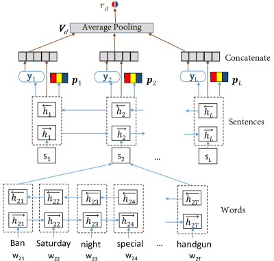
Figure 1: Hierarchical bi-LSTM for joint sentence–document analysis ($\mathbf{y}_{i}$ denotes the predicted 57-class distribution of sentence $s_{i}$; $\mathbf{p}_{i}$ denotes the distribution over left (in red), right (in blue) and neutral (in yellow); ${r}_{d}$ denotes the RILE score of $d$).

4 Manifesto Position Re-ranking

We leverage party-level information to enforce smoothness and regularity in manifesto positioning on the left–right spectrum Greene (2016). For example, manifestos released by parties in a coalition are more likely to be closer in RILE score, and a party’s position in an election is often a relative shift from its position in earlier election, so temporal information can provide smoother estimations.

PSLcoal — Coalition features
$\mathtt{Manifesto(x)}\wedge\mathtt{Party(x,a)}\wedge\mathtt{Manifesto(y)}\wedge\mathtt{Party(y,b)}\wedge\mathtt{SameElec(x,y)}\wedge\mathtt{RegCoalition(a,b)}\wedge\mathtt{pos(x)}\rightarrow\mathtt{pos(y)}$
$\mathtt{Manifesto(x)}\wedge\mathtt{Party(x,a)}\wedge\mathtt{Manifesto(y)}\wedge\mathtt{Party(y,b)}\wedge\mathtt{SameElec(x,y)}\wedge\mathtt{RegCoalition(a,b)}\wedge\neg\mathtt{pos(x)}\rightarrow\neg\mathtt{pos(y)}$
$\mathtt{Manifesto(x)}\wedge\mathtt{Party(x,a)}\wedge\mathtt{Manifesto(y)}\wedge\mathtt{Party(y,b)}\wedge\mathtt{Recent(x,y)}\wedge\mathtt{EUCoalition(a,b)}\wedge\mathtt{pos(x)}\rightarrow\mathtt{pos(y)}$
$\mathtt{Manifesto(x)}\wedge\mathtt{Party(x,a)}\wedge\mathtt{Manifesto(y)}\wedge\mathtt{Party(y,b)}\wedge\mathtt{Recent(x,y)}\wedge\mathtt{EUCoalition(a,b)}\wedge\neg\mathtt{pos(x)}\rightarrow\neg\mathtt{pos(y)}$
Transitivity
$\begin{array}[]{l}\mathtt{Manifesto(x)}\wedge\mathtt{Party(x,a)}\wedge\mathtt{Manifesto(y)}\wedge\mathtt{Party(y,b)}\wedge\mathtt{Manifesto(z)}\wedge\mathtt{Party(z,c)}\quad\wedge\\ \mathtt{SameElec(x,y)}\wedge\mathtt{SameElec(y,z)}\wedge\mathtt{RegCoalition(a,b)}\wedge\mathtt{RegCoalition(b,c)}\wedge\mathtt{pos(x)}\end{array}\rightarrow\text{pos(z)}$
$\begin{array}[]{l}\mathtt{Manifesto(x)}\wedge\mathtt{Party(x,a)}\wedge\mathtt{Manifesto(y)}\wedge\mathtt{Party(y,b)}\wedge\mathtt{Manifesto(z)}\wedge\mathtt{Party(z,c)}\quad\wedge\\ \mathtt{SameElec(x,y)}\wedge\mathtt{SameElec(y,z)}\wedge\mathtt{RegCoalition(a,b)}\wedge\mathtt{RegCoalition(b,c)}\wedge\neg\mathtt{pos(x)}\end{array}\rightarrow\neg\mathtt{pos(z)}$
$\begin{array}[]{l}\mathtt{Manifesto(x)}\wedge\mathtt{Party(x,a)}\wedge\mathtt{Manifesto(y)}\wedge\mathtt{Party(y,b)}\wedge\mathtt{Manifesto(z)}\wedge\mathtt{Party(z,c)}\quad\wedge\\ \mathtt{Recent(x,y)}\wedge\mathtt{Recent(y,z)}\wedge\mathtt{EUCoalition(a,b)}\wedge\mathtt{EUCoalition(b,c)}\wedge\mathtt{pos(x)}\end{array}\rightarrow\text{pos(z)}$
$\begin{array}[]{l}\mathtt{Manifesto(x)}\wedge\mathtt{Party(x,a)}\wedge\mathtt{Manifesto(y)}\wedge\mathtt{Party(y,b)}\wedge\mathtt{Manifesto(z)}\wedge\mathtt{Party(z,c)}\quad\wedge\\ \mathtt{Recent(x,y)}\wedge\mathtt{Recent(y,z)}\wedge\mathtt{EUCoalition(a,b)}\wedge\mathtt{EUCoalition(b,c)}\wedge\neg\mathtt{pos(x)}\end{array}\rightarrow\neg\mathtt{pos(z)}$
PSLesim — Similarity-based relational feature
$\mathtt{Manifesto(x)}\wedge\mathtt{Manifesto(y)}\wedge\mathtt{Similarity(x,y)}\wedge\mathtt{Recent(x,y)}\wedge\mathtt{pos(x)}\rightarrow\mathtt{pos(y)}$
$\mathtt{Manifesto(x)}\wedge\mathtt{Manifesto(y)}\wedge\mathtt{Similarity(x,y)}\wedge\mathtt{Recent(x,y)}\wedge\neg\mathtt{pos(x)}\rightarrow\neg\mathtt{pos(y)}$
PSLploc — Right–left ratio
$\mathtt{Manifesto(x)}\wedge\mathtt{LwRightLeftRatio(x)}\rightarrow\mathtt{pos(x)}$
$\mathtt{Manifesto(x)}\wedge\neg\mathtt{LwRightLeftRatio(x)}\rightarrow\neg\mathtt{pos(x)}$
PSLtemp— Temporal Dependency
$\mathtt{Manifesto(x)}\wedge\mathtt{Party(x,a)}\wedge\mathtt{PreviousManifesto(x,a,t)}\wedge\mathtt{pos(t)}\rightarrow\mathtt{pos(x)}$
$\mathtt{Manifesto(x)}\wedge\mathtt{Party(x,a)}\wedge\mathtt{PreviousManifesto(x,a,t)}\wedge\neg\mathtt{pos(t)}\rightarrow\neg\mathtt{pos(x)}$

Table 1: PSL Model: Values for $\mathtt{Similarity}$, $\mathtt{LwRightLeftRatio}$ and $\mathtt{pos}$ are obtained from the joint-structured model (Figure 1). Except for $\mathtt{pos}$, other values are fixed in the network. Domain ($\mathtt{y}$) for $\mathtt{SameElec(x,y)}$ is within the country, and for $\mathtt{Recent(x,y)}$ covers all the countries. $\neg$ denotes negation. Distance to satisfaction for each ground rule is obtained using a hinge-loss potential, which is then used inside the HL-MRF model (Equation (5)), where $\mathtt{pos}$ is $\mathbf{Y}$.

4.1 Probabilistic Soft Logic

To address this, we propose an approach using hinge-loss Markov random fields (“HL-MRFs”), a scalable class of continuous, conditional graphical models Bach et al. (2013). HL-MRFs have been used for many tasks including political framing analysis on Twitter Johnson et al. (2017) and user stance classification on socio-political issues Sridhar et al. (2014). These models can be specified using Probabilistic Soft Logic (“PSL”) Bach et al. (2015), a weighted first order logical template language. An example of a PSL rule is

$$\lambda:\mathtt{P(a)}\wedge\mathtt{Q(a,b)}\rightarrow\mathtt{R(b)}$$

where $\mathtt{P}$, $\mathtt{Q}$, and $\mathtt{R}$ are predicates, $\mathtt{a}$ and $\mathtt{b}$ are variables, and $\lambda$ is the weight associated with the rule. PSL uses soft truth values for predicates in the interval $\big{[}0,1\big{]}$. The degree of ground rule satisfaction is determined using the Lukasiewicz t-norm and its corresponding co-norm as the relaxation of the logical AND and OR, respectively. The weight of the rule indicates its importance in the HL-MRF probabilistic model, which defines a probability density function of the form:

$$\begin{split}P(\mathbf{Y}|\mathbf{X})&\propto\exp\left(-\sum_{r=1}^{M}\lambda_{r}\phi_{r}(\mathbf{Y},\mathbf{X})\right),\\ \phi_{r}(\mathbf{Y},\mathbf{X})&=\max{\{l_{r}(\mathbf{Y},\mathbf{X}),0\}}^{\rho_{r}},\end{split}$$ (5)

where $\phi_{r}$($\mathbf{Y},\mathbf{X}$) is a hinge-loss potential corresponding to an instantiation of a rule, and is specified by a linear function $l_{r}$ and optional exponent $\rho_{r}$ $\in\{1,2\}$. Note that the hinge-loss potential captures the distance to satisfaction.

4.2 PSL Model

Here we elaborate our PSL model (given in Table 1) based on coalition information, manifesto content-based features (manifesto similarity and right–left ratio), and temporal dependency. Our target $\mathtt{pos}$ (calibrated RILE) is a continuous variable $\big{[}0,1\big{]}$, where 1 indicates that a manifesto occupies an extreme right position, 0 denotes an extreme left position, and 0.5 indicates center. Each instance of a manifesto and its party affiliation are denoted by the predicates $\mathtt{Manifesto}$ and $\mathtt{Party}$.

Coalition: We model multi-relational networks based on regional coalitions within a given country ($\mathtt{RegCoalition}$), and also cross-country coalitions in the European parliament ($\mathtt{EUCoalition}$). We set the scope of interaction between manifestos ($\mathtt{x}$ and $\mathtt{y}$) from a country to the same election ($\mathtt{SameElec}$). For manifestos across countries, we consider only the most recent manifesto ($\mathtt{Recent}$) from each party ($\mathtt{y}$), released within 4 years relative to $\mathtt{x}$. We use a logistic transformation of the number of times two parties have been in a coalition in the past (to get a value between 0 and 1), for both $\mathtt{RegCoalition}$ and $\mathtt{EUCoalition}$. We also construct rules based on transitivity for both the relational features, i.e., parties which have had common coalition partners, even if they were not allies themselves, are likely to have similar policy positions.

Manifesto similarity: Manifestos that are similar in content are expected to have similar RILE scores (and associated sentence-level label distributions), similar to the modeling intuition captured by Burford et al. (2015) in the context of congressional debate vote prediction. For a pair of recent manifestos ($\mathtt{Recent}$) we use the cosine similarity ($\mathtt{Similarity}$) between their respective document vectors $\mathbf{V_{d}}$ (Figure 1).

Right–left ratio: For a given manifesto, we compute the ratio of sentences categorized under right to others ($\frac{\textsc{\# right}}{\textsc{\# right}+\textsc{\# left}+\textsc{\# neutral}})$, where the categorization for sentences is obtained using the joint-structured model (Equation (4)). We also encode the location of sentence $l_{s}$ in a document, by weighing the count of sentences for each class $C$ by its location value $\sum_{s\in C}\log(l_{s}+1)$ (referred to as loc_lr). The intuition here is that the beginning parts of a manifesto tends to contain generic information such as preamble, compared to later parts which are more policy-dense. We perform a logistic transformation of loc_lr to derive the $\mathtt{LwRightLeftRatio}$.

Temporal dependency: We capture the temporal dependency between a party’s current manifesto position and its previous manifesto position ($\mathtt{PreviousManifesto}$).

Other than for the look-up based random variables, the network is instantiated with predictions (for $\mathtt{Similarity}$, $\mathtt{LwRightLeftRatio}$ and $\mathtt{pos}$) from the joint-structured model (Figure 1). All the random variables, except $\mathtt{pos}$ (which is the target variable), are fixed in the network. These values are then used inside a PSL model for collective probabilistic reasoning, where the first-order logic given in Table 1 is used to define the graphical model (HL-MRF) over the random variables detailed above. Inference on the HL-MRF is used to obtain the most probable interpretation such that it satisfies most ground rule instances, i.e., considering the relational and temporal dependencies.

5 Evaluation

5.1 Experimental Setup

As our dataset, we use manifestos from CMP for European countries only, as in Section 5.5 we will validate the manifesto’s overall position on the left-right spectrum, using the Chapel Hill Expert Survey (CHES), which is only available for European countries Bakker et al. (2015). In this, we sample 1004 manifestos from 12 European countries, written in 10 different languages — Danish (Denmark), Dutch (Netherlands), English (Ireland, United Kingdom), Finnish (Finland), French (France), German (Austria, Germany), Italian (Italy), Portuguese (Portugal), Spanish (Spain), and Swedish (Sweden). Out of the 1004 manifestos, 272 are annotated with both sentence-level labels and RILE scores, and the remainder only have RILE scores (see Table 2 for further statistics).

There are (less) scenarios where a natural sentence is segmented into sub-sentences and annotated with different classes Däubler et al. (2012). Hence we use NLTK sentence tokenizer followed by heuristics from Däubler et al. (2012) to obtain sub-sentences. Consistent with previous work Subramanian et al. (2017), we present results with manually segmented and annotated test documents.

Lang.	# Docs (Anntd.)	# Sents (Anntd.)
Danish	175    (36)	29694      (8762)
Dutch	107    (48)	132524   (70559)
English	117    (27)	86603   (34512)
Finnish	97    (16)	17979      (8503)
French	53    (10)	22747      (5559)
German	117    (46)	111376   (73652)
Italian	98    (15)	41455      (5154)
Portuguese	60       (9)	40922   (11077)
Spanish	85    (50)	145355   (93964)
Swedish	95    (15)	19551      (7938)
Total	1004 (272)	648206 (319680)

Table 2: Statistics of dataset (“Anntd.” refers to the number of documents with sentence annotations in the second column, and the number of sentences with annotations in the third column).

5.2 Baseline Approaches

Sentence-level baseline approaches include:

• BoW-NN: TF-IDF-weighted unigram bag-of-words representation of sentences Biessmann (2016), and monolingual training using a multi-layer perceptron (“MLP”) model.

• BoT-NN: Similar to above, but trigram bag-of-words.

• AE-NN: MLP model with average multilingual word embeddings as the sentence representation Subramanian et al. (2017).

• CNN: Convolutional neural network (“CNN”: Glavaš et al. (2017a)) with multilingual word embeddings.

• Bi-LSTM: Simple bi-LSTM over multilingual word embeddings, last hidden units are concatenated to form the sentence representation, and fed directly into a softmax sentence-level layer. We evaluate two scenarios: (1) with a trainable embedding matrix $W_{e}$ (Bi-LSTM(+up)); and (2) without a trainable $W_{e}$.

Document-level baseline approaches include:

• BoC: Bag-of-centroids (BoC) document representation based on clustering the word embeddings Lebret and Collobert (2014), fed into a neural network regression model.

• HCNN: Hierarchical CNN, where we encode both the sentence and document using stacked CNN layers.

• HNN: State-of-the-art hierarchical neural network model of Subramanian et al. (2017), based on average embedding representations for sentences and the document.

We present results evaluated under two different settings: (a) 80–20% random split averaged across 10 runs to validate the hierarchical model (Section 5.3 and Section 5.4); and (b) temporal setting, where train- and test-set are split chronologically, to validate both the hierarchical deep model and the PSL approach especially, since we encode temporal dependencies (Section 5.5).

5.3 Hierarchical Sentence- and Document-level Model

Lang.	BoW-NN	BoT-NN	AE-NN	CNN	Bi-LSTM	Bi-LSTM(+up)	Joint${}_{\text{sent}}$	Joint	Joint${}_{\text{struc}}$
Danish	0.35	0.33	0.35	0.31	0.38	0.38	0.44	0.40	0.43
Dutch	0.41	0.41	0.40	0.34	0.39	0.43	0.52	0.50	0.50
English	0.39	0.43	0.43	0.40	0.45	0.47	0.49	0.50	0.49
Finnish	0.30	0.34	0.33	0.30	0.38	0.39	0.44	0.41	0.42
French	0.36	0.37	0.36	0.37	0.42	0.44	0.48	0.49	0.48
German	0.33	0.35	0.37	0.35	0.40	0.41	0.45	0.45	0.46
Italian	0.33	0.38	0.37	0.31	0.37	0.39	0.49	0.52	0.52
Portuguese	0.32	0.38	0.31	0.28	0.43	0.46	0.44	0.44	0.43
Spanish	0.38	0.39	0.39	0.35	0.42	0.41	0.50	0.49	0.50
Swedish	0.46	0.42	0.36	0.36	0.41	0.44	0.49	0.46	0.46
Avg.	0.36	0.38	0.38	0.35	0.40	0.42	0.48	0.47	0.48

Table 3: Micro-Averaged F-measure for sentence classification. Best scores are given in bold.

We present sentence-level results with a 80–20% random split in Table 3, stratified by country, averaged across 10 runs. For Bi-LSTM, we found the setting with a trainable embedding matrix (Bi-LSTM(+up)) to perform better than the non-trainable case (Bi-LSTM). Hence we use a similar setting for Joint and Joint${}_{\text{struc}}$. We show the effect of $\alpha$ (from Equation (2)) in Figure 2(a), based on which we set $\alpha=0.3$ hereafter. With the chosen model, we study the effect of the structured loss (Equation (4)), by varying $\gamma$ with fixed $\beta=0.1$, as shown in Figure 2(b). We observe that $\gamma=0.7$ gives the best performance, and varying $\beta$ with $\gamma$ at 0.7 does not result in any further improvement (see Figure 2(c)). Sentence-level results measured using F-measure, for baseline approaches and the proposed models selected from Figure 2(a) (Joint), Figures 2(b) and 2(c) (Joint${}_{\text{struc}}$) are given in Table 3. We also evaluate the special case of $\alpha=1$, in the form of sentence-only model Joint${}_{\text{sent}}$. For the document-level task, results for overall manifesto positioning measured using Pearson’s correlation ($r$) and Spearman’s rank correlation ($\rho$) are given in Table 4. We also evaluate the hierarchical bi-LSTM model with document-level objective only, Joint${}_{\text{doc}}$.

Approach	$r$	$\rho$
BoC	0.18	0.20
HCNN	0.24	0.26
HNN	0.28	0.32
Joint${}_{\text{doc}}$	0.30	0.37
Joint	0.46	0.54
Joint${}_{\text{struc}}$	0.50	0.63

Table 4: RILE score prediction performance. Best scores are given in bold.

We observe that hierarchical modeling (Joint${}_{\text{sent}}$, Joint and Joint${}_{\text{struc}}$) gives the best performance for sentence-level classification for all the languages except Portuguese, on which it performs slightly worse than Bi-LSTM(+up). Also, Joint${}_{\text{struc}}$, does not improve over Joint${}_{\text{sent}}$. We perform further analysis to see the effect of joint-structured model on the sentence-level task under sparsely-labeled conditions in Section 5.4. On the other hand, for the document-level task, the joint model (Joint) performs better than Joint${}_{\text{doc}}$ and all the baseline approaches. Lastly, the joint-structured model (Joint${}_{\text{struc}}$) provides further improvement over Joint.

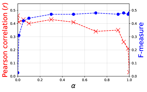
(a) Effect of $\alpha$ in equation 2.

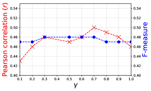
(b) Effect of $\gamma$ in equation 4.

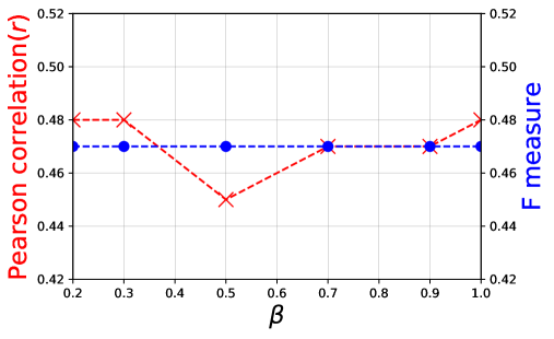
(c) Effect of $\beta$ in equation 4.

Figure 2: Effect of hyper-parameters on sentence- and document-level performance. denotes F-measure (right axis) and $\times$ denotes Pearson correlation (left axis).

5.4 Analysis of Joint-Structured Model for Sentence-level task

To understand the utility of joint modeling, especially given that there are more manifestos with document-level labels only than both sentence- and document-level labels, we compare the following two settings: (1) Joint${}_{\text{struc}}$, which uses additional manifestos with document-level supervision (RILE); and (2) Joint${}_{\text{sent}}$, which uses manifestos with sentence-level supervision only. We vary the proportion of labeled documents at the sentence-level, from 10% to 80%, to study the effect under sparsely-labeled conditions. Note that 80% is the maximum labeled training data under the cross-validation setting. In other cases, a subset (say 10%) is randomly sampled for training. From Figure 3, having more manifestos with document-level supervision demonstrates the advantage of semi-supervised learning, especially when the sentence-level supervision is sparse ($\leq$ 40%)— Joint${}_{\text{struc}}$ performs better than Joint${}_{\text{sent}}$.

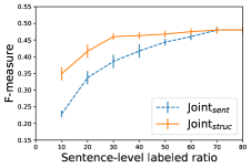
Figure 3: F-measure for Joint${}_{\text{struc}}$ vs. Joint${}_{\text{sent}}$ across different ratios of sentence-level labeled manifestos (averaged over 10 runs, with standard deviation)

5.5 Manifesto Position Re-ranking using PSL

Finally, we present the results using PSL, which calibrates the overall manifesto position on the left–right spectrum, obtained using the joint-structured model (Joint${}_{\text{struc}}$). As we evaluate the effect of temporal dependency, we use manifestos before 2008-09 for training (868 in total) and the later ones (until 2015, 136 in total) for testing. This test set covers one recent set of election manifestos for most countries, and two for the Netherlands, Spain and United Kingdom. To avoid variance in right-to-left ratio and the target variable ($\mathtt{pos}$, initialized using Joint${}_{\text{struc}}$) between the training and test sets, we build a stacked network Fast and Jensen (2008), whereby we estimate values for the training set using cross-validation across the training partition, and estimate values for the test-set with a model trained over the entire training data. Note that we build the Joint${}_{\text{struc}}$ model afresh using the chronologically split training set, and the parameters are tuned again using an 80-20 random split of the training set. For a consistent view of results for both the tasks (and stages), we provide micro-averaged results for sentence-classification with the competing approaches (from Table 3): AE-NN Subramanian et al. (2017), Bi-LSTM(+up), and Joint${}_{\text{struc}}$. Results are presented in Table 5, noting that the results for a given method will differ from earlier due to the different data split.

Approach	F-measure
AE-NN	0.31
Bi-LSTM(+up)	0.36
Joint${}_{\text{struc}}$	0.42

Table 5: Micro-averaged F-measure for manifestos released after 2008-09. Best scores are given in bold.

For the document-level regression task, we also evaluate other approaches based on manifesto similarity and automated scaling with sentence-level policy positions:

• Cross-lingual scaling (CLS): A recent unsupervised approach for crosslingual political speech text scoring Glavaš et al. (2017b), based on TF-IDF weighed average word-embeddings to represent documents, and a graph constructed using pair-wise document similarity. Given two pivot texts (for left and right), label propagation approach is used to position other documents.

• PCA: Apply principal component analysis Gabel and Huber (2000) on the distribution of sentence-level policy positions (56 classes, without 000), and use the projection on its principal component to explain maximum variance in its sentence-level positions, as a latent manifesto-level position score.

• Joint${}_{\text{struc}}$: We evaluate the scores obtained using Joint${}_{\text{struc}}$, which we calibrate using PSL.

We validate the calibrated position scores using both RILE and CHES scores. We use CHES 2010-14, and map the manifestos to the closest survey year (wrt its election date). CHES scores are used only for evaluation and not during training. We provide results in Table 6 by augmenting features for the PSL model (Table 1) incrementally. We observed that the coalition-based feature, and polarity of sentences with its position information improves the overall ranking ($r$, $\rho$). Document similarity based relational feature provides only mild improvement (similarly to Burford et al. (2015)), and temporal dependency provides further improvement against CHES. That is, combining content, network and temporal features provides the best results.

	RILE			CHES
	$r$	$\rho$		$r$	$\rho$
CLS	0.11	0.10		0.09	$-$0.07
PCA	0.26	0.17		0.01	$-$0.02
Joint${}_{\text{struc}}$	0.46	0.42		0.42	$-$0.42
PSL${}_{\text{coal}}$	0.51	0.45		0.49	$-$0.45
PSL${}_{\text{coal + esim}}$	0.52	0.47		0.50	$-$0.46
PSL${}_{\text{coal + esim + ploc}}$	0.54	0.56		0.53	$-$0.56
PSL${}_{\text{coal + esim + ploc + temp}}$	0.54	0.57		0.55	$-$0.61

Table 6: Manifesto regression task using the two-stage approach. Best scores are given in bold.

6 Conclusion and Future Work

This work has been targeted at both fine- and coarse-grained manifesto text position analysis. We have proposed a two-stage approach, where in the first step we use a hierarchical multi-task deep model to handle the sentence- and document-level tasks together. We also utilize additional information on label structure, to augment an auxiliary structured loss. Since the first step places the manifesto on the left–right spectrum using text only, we leverage context information, such as coalition and temporal dependencies to calibrate the position further using PSL. We observed that: (a) a hierarchical bi-LSTM model performs best for the sentence-level classification task, offering a 10% improvement over the state-of-art approach Subramanian et al. (2017); (b) modeling the document-level task jointly, and also augmenting the structured loss, gives the best performance for the document-level task and also helps the sentence-level task under sparse supervision scenarios; and (c) the inclusion of a calibration step with PSL provides significant gains in performance against both RILE and CHES, in the form of an increase from $\rho=0.42$ to 0.61 wrt CHES survey scores.

There are many possible extensions to this work, including: (a) learning multilingual word embeddings with domain information; and (b) modeling other policy related scores from text, such as “support for EU integration”.

References

- Artetxe et al. (2016) Mikel Artetxe, Gorka Labaka, and Eneko Agirre. 2016. Learning principled bilingual mappings of word embeddings while preserving monolingual invariance. In Proceedings of the 2016 Conference on Empirical Methods in Natural Language Processing. EMNLP, pages 2289–2294.
- Bach et al. (2015) S. H. Bach, B. Huang M. Broecheler, and L. Getoor. 2015. Hinge-loss markov random fields and probabilistic soft logic. CoRR abs/1505.04406.
- Bach et al. (2013) Stephen H. Bach, Bert Huang, Ben London, and Lise Getoor. 2013. Hinge-loss markov random fields: Convex inference for structured prediction. In Proceedings of the Twenty-Ninth Conference on Uncertainty in Artificial Intelligence.
- Bakker et al. (2015) Ryan Bakker, Catherine De Vries, Erica Edwards, Liesbet Hooghe, Seth Jolly, Gary Marks, Jonathan Polk, Jan Rovny, Marco Steenbergen, and Milada Anna Vachudova. 2015. Measuring party positions in europe: The chapel hill expert survey trend file, 1999–2010. Party Politics 21(1):143–152.
- Benoit and Laver (2007) Kenneth Benoit and Michael Laver. 2007. Estimating party policy positions: Comparing expert surveys and hand-coded content analysis. Electoral Studies 26(1):90–107.
- Biessmann (2016) Felix Biessmann. 2016. Automating political bias prediction. CoRR abs/1608.02195.
- Bojanowski et al. (2017) Piotr Bojanowski, Edouard Grave, Armand Joulin, and Tomas Mikolov. 2017. Enriching word vectors with subword information. Transactions of the Association for Computational Linguistics 5:135–146.
- Bruinsma and Gemenis (2017) B. Bruinsma and K. Gemenis. 2017. Validating Wordscores. CoRR abs/1707.04737.
- Budge et al. (2001) I Budge, H.D Klingemann, A Volkens, J Bara, E Tannenbaum, R Fording, D Hearl, H.M Kim, M McDonald, and S Mendes. 2001. Mapping Policy Preferences: Parties, Electors and Governments. Oxford University Press.
- Burford et al. (2015) Clint Burford, Steven Bird, and Timothy Baldwin. 2015. Collective document classification with implicit inter-document semantic relationships. In Proceedings of the Fourth Joint Conference on Lexical and Computational Semantics (*SEM 2015). Denver, USA, pages 106–116.
- Däubler and Benoit (2017) Thomas Däubler and Kenneth Benoit. 2017. Estimating better left-right positions through statistical scaling of manual content analysis. Retrieved from http://kenbenoit.net/pdfs/text_in_context_2017.pdf .
- Däubler et al. (2012) Thomas Däubler, Kenneth Benoit, Slava Mikhaylov, and Michael Laver. 2012. Natural sentences as valid units for coded political texts. British Journal of Political Science 42(4):937–951.
- Fast and Jensen (2008) Andrew Fast and David Jensen. 2008. Why stacked models perform effective collective classification. In Proceedings of the Eighth International Conference on Data Mining. IEEE, pages 785–790.
- Gabel and Huber (2000) Matthew J Gabel and John D Huber. 2000. Putting parties in their place: Inferring party left-right ideological positions from party manifestos data. American Journal of Political Science pages 94–103.
- Glavaš et al. (2017a) Goran Glavaš, Federico Nanni, and Simone Paolo Ponzetto. 2017a. Cross-lingual classification of topics in political texts. In Proceedings of the Second Workshop on NLP and Computational Social Science. ACL, pages 42–46.
- Glavaš et al. (2017b) Goran Glavaš, Federico Nanni, and Simone Paolo Ponzetto. 2017b. Unsupervised cross-lingual scaling of political texts. In Proceedings of the 15th Conference of the European Chapter of the Association for Computational Linguistics: Volume 2, Short Papers. volume 2, pages 688–693.
- Graves et al. (2013) Alex Graves, Abdel-rahman Mohamed, and Geoffrey Hinton. 2013. Speech recognition with deep recurrent neural networks. In Proceedings of the international conference on Acoustics, speech and signal processing (ICASSP). IEEE, pages 6645–6649.
- Greene (2016) Zachary Greene. 2016. Competing on the issues: How experience in government and economic conditions influence the scope of parties’ policy messages. Party Politics 22(6):809–822.
- Grimmer and Stewart (2013) Justin Grimmer and Brandon M Stewart. 2013. Text as data: The promise and pitfalls of automatic content analysis methods for political texts. Political analysis 21(3):267–297.
- Hjorth et al. (2015) Frederik Georg Hjorth, Robert Tranekær Klemmensen, Sara Binzer Hobolt, Martin Ejnar Hansen, and Peter Kurrild-Klitgaard. 2015. Computers, coders, and voters: Comparing automated methods for estimating party positions. Research and Politics 2(2):1–9.
- Hochreiter and Schmidhuber (1997) Sepp Hochreiter and Jürgen Schmidhuber. 1997. Long short-term memory. Neural Computation 9(8):1735–1780.
- Johnson et al. (2017) Kristen Johnson, Di Jin, and Dan Goldwasser. 2017. Leveraging behavioral and social information for weakly supervised collective classification of political discourse on twitter. In Proceedings of the Association for Computational Linguistics. ACL, pages 741–752.
- Jou and Dalton (2017) Willy Jou and Russell J. Dalton. 2017. Left-right orientations and voting behavior. Oxford Research Encyclopedia of Politics .
- Klingemann et al. (2006) Hans-Dieter Klingemann, Andrea Volkens, Judith Bara, Ian Budge, and Michael McDonald. 2006. Mapping Policy Preferences II. Estimates for Parties, Electors, and Governments in Eastern Europe, European Union, and OECD. Oxford University Press.
- Lazer et al. (2009) David Lazer, Alex Sandy Pentland, Lada Adamic, Sinan Aral, Albert Laszlo Barabasi, Devon Brewer, Nicholas Christakis, Noshir Contractor, James Fowler, Myron Gutmann, et al. 2009. Life in the network: the coming age of computational social science. Science (New York, NY) 323(5915):721.
- Lebret and Collobert (2014) Rémi Lebret and Ronan Collobert. 2014. N-gram-based low-dimensional representation for document classification. CoRR abs/1412.6277.
- Li et al. (2015) Jiwei Li, Luong Minh-Thang, and Jurafsky Dan. 2015. A hierarchical neural autoencoder for paragraphs and documents. In Proceedings of the 53rd Annual Meeting of the Association for Computational Linguistics and the 7th International Joint Conference on Natural Language Processing. ACL, pages 1106––1115.
- Lo et al. (2013) James Lo, Sven-Oliver Proksch, and Thomas Gschwend. 2013. A common left-right scale for voters and parties in europe. Political Analysis 22(2):205–223.
- Lowe et al. (2011) Will Lowe, Kenneth Benoit, Slava Mikhaylov, and Michael Laver. 2011. Scaling policy preferences from coded political texts. Legislative studies quarterly 36(1):123–155.
- McDonald et al. (2007) Ryan McDonald, Kerry Hannan, Tyler Neylon, Mike Wells, and Jeff Reynar. 2007. Structured models for fine-to-coarse sentiment analysis. In Proceedings of the 45th annual meeting of the association of computational linguistics. ACL, pages 432–439.
- Menini et al. (2017) Stefano Menini, Federico Nanni, Simone Paolo Ponzetto, and Sara Tonelli. 2017. Topic-based agreement and disagreement in us electoral manifestos. In Proceedings of the 2017 Conference on Empirical Methods in Natural Language Processing. EMNLP, pages 2938–2944.
- Merz et al. (2016) Nicolas Merz, Sven Regel, and Jirka Lewandowski. 2016. The manifesto corpus: A new resource for research on political parties and quantitative text analysis. Research & Politics 3(2).
- Mikhaylov et al. (2012) Slava Mikhaylov, Michael Laver, and Kenneth R Benoit. 2012. Coder reliability and misclassification in the human coding of party manifestos. Political Analysis 20(1):78–91.
- Mohammad et al. (2017) Saif M Mohammad, Parinaz Sobhani, and Svetlana Kiritchenko. 2017. Stance and sentiment in tweets. ACM Transactions on Internet Technology (TOIT) 17(3):26.
- Slapin and Proksch (2008) Jonathan B Slapin and Sven-Oliver Proksch. 2008. A scaling model for estimating time-series party positions from texts. American Journal of Political Science 52(3):705–722.
- Smith et al. (2017) Samuel L Smith, Turban David HP, Hamblin Steven, and Hammerla Nils Y. 2017. Offline bilingual word vectors, orthogonal transformations and the inverted softmax. In Proceedings of the 5th International Conference on Learning Representations (ICLR).
- Sridhar et al. (2014) Dhanya Sridhar, Lise Getoor, and Marilyn Walker. 2014. Collective stance classification of posts in online debate forums. In Proceedings of the Joint Workshop on Social Dynamics and Personal Attributes in Social Media. ACL, pages 109–117.
- Subramanian et al. (2017) Shivashankar Subramanian, Trevor Cohn, Timothy Baldwin, and Julian Brooke. 2017. Joint sentence-document model for manifesto text analysis. In Proceedings of the 15th Annual Workshop of The Australasian Language Technology Association. ALTA, pages 25–33.
- Verberne et al. (2014) Suzan Verberne, Eva D’hondt, Antal van den Bosch, and Maarten Marx. 2014. Automatic thematic classification of election manifestos. Information Processing & Management 50(4):554–567.
- Volkens et al. (2013) Andrea Volkens, Judith Bara, Budge Ian, and Simon Franzmann. 2013. Understanding and validating the left-right scale (RILE). In Mapping Policy Preferences From Texts: Statistical Solutions for Manifesto Analysts, Oxford University Press, chapter 6.
- Volkens et al. (2017) Andrea Volkens, Pola Lehmann, Theres Matthieß, Nicolas Merz, Sven Regel, and Bernhard Weßels. 2017. The Manifesto Data Collection. Manifesto Project (MRG/CMP/MARPOR). Version 2017b. Wissenschaftszentrum Berlin für Sozialforschung, Berlin, Germany.
- Zirn et al. (2016) Cäcilia Zirn, Goran Glavaš, Federico Nanni, Jason Eichorts, and Heiner Stuckenschmidt. 2016. Classifying topics and detecting topic shifts in political manifestos. In Proceedings of the International Conference on the Advances in Computational Analysis of Political Text. PolText, pages 88–93.