Cosmological Model Independent Time Delay Method

Abstract

We propose a Cosmological Model Independent Time Delay (CMITD) method where the Lorentz invariance violation (LIV) variable $K(z)$ is constructed by observational data instead of cosmological model. The simulated time delay data show the CMITD method could present the validity of LIV test. And, the errors in the propagating process is critical for the existence and magnitude of LIV.

1 Introduction

Lorentz invariance is the cornerstone of modern physics. As a non-general symmetry, the violation of Lorentz symmetry is expected in quantum gravity frameworks. And Lorentz invariance violation (LIV) deduces a deformed energy-momentum relation in the high energy scale often around Planck scale [1, 2, 3, 4]. As the velocities of photons are changed, it is also called modified dispersion relation. Then, the simplest test of LIV is the arrival-time differences of photons in astrophysics. Two photons of different energies in the LIV background would lead to different arrival times which is called time delay, even they emitted simultaneously from the same remote cosmological source.

Theoretically, LIV is caused by the quantum gravities which have to modify General Relativity (GR). Meanwhile, the LIV effect is small but could be directly applied to kinematic process luckily. Gamma-ray bursts (GRBs) are suitable for this kinematic studies with the distant transient properties [5, 6, 7, 8, 9, 10]. Moreover, the kinematic process needs to consider the late acceleration in our universe which could be explained as dark energy model or modified gravity model. Lorentz symmetry are invariant in the cosmological model with GR background. The dark energy models with GR background are used for LIV test in literatures [11, 12, 13, 14, 15]. However, the whole LIV test scenario is self-contradictory if the cosmological model in GR was used.

In this paper, we calculate the time delay term by using observational data instead of cosmological model. We call it Cosmological Model Independent Time Delay (CMITD) method. The paper is arranged as below. In Section 2, the LIV theories are introduced. In Section 3, we show the contradictions in theories and our CMITD solution. In Section 4, the results of LIV test are presented and discussed. Finally, we give a short summary in Section 5.

2 Lorentz Invariance Violation Theory

In General Relativity, the trajectory of the massless particle with dispersion relation $E=p^{2}c^{2}$ which shows the velocity of photon is constant and does not have LIV [16]. Violations of local Lorentz invariance modify the dispersion relation [17]. The broken energy scale named $E_{LV}$ is usually assumed around the Planck scale. When examining particles with energies much smaller than the symmetry breaking scale, we may choose only the leading order correction phenomenally. Assuming the leading LIV correction is of order $n$, the LIV model can be described as

$$E^{2}=p^{2}c^{2}\times[1-s_{\pm}(\frac{E}{E_{LV}})^{n}],$$ (2.1)

where $s_{\pm}=+1/s_{\pm}=-1$ corresponds the subluminal/superluminal case [10].

Then, the modified velocity of photon is given by

$$v=\frac{\partial E}{\partial p}=c[1-s_{\pm}\frac{n+1}{2}(\frac{E}{E_{LV}})^{n}].$$ (2.2)

And, the energy varying velocities deduce a time delay [14]

$$\Delta t_{LV}=t_{h^{*}}-t_{l^{*}}=s_{\pm}\frac{(1+n)(E_{h^{*}}^{n}-E_{l^{*}}^{n})}{2H_{0}E_{LV}^{n}}\int_{0}^{z}\frac{(1+z^{\prime})^{n}}{h(z^{\prime})}dz^{\prime},$$ (2.3)

where the index $h^{*}$ ($l^{*}$) denotes high (low) energy, $E_{h^{*}}$ and $E_{l^{*}}$ are dependent on experiments, $h(z)=H(z)/H_{0}$ with $H(z)$ as the Hubble parameter and the index $0$ denotes today’s value. For latter convenience, we define the LIV parameter $a_{LV}$ and the LIV variable $K(z)$ as

$$a_{LV}=s_{\pm}\frac{(1+n)(E_{h^{*}}^{n}-E_{l^{*}}^{n})}{2H_{0}E_{LV}^{n}},$$ (2.4)

$$K(z)=\int_{0}^{z}\frac{(1+z^{\prime})^{n}}{h(z^{\prime})}dz^{\prime}.$$ (2.5)

According to Eq.(2.2), we could have $|1-v/c|\sim a_{LV}H_{0}$ where $H_{0}$ is canceled by $a_{LV}$. The value of $|1-v/c|$ and $E_{LV}$ are independent of $H_{0}$ intrinsically. And, in this paper, our definition of $K(z)$ is different from the $K(z)$ in Ref.[12] by a factor of $1/(1+z)$ for convience. Moreover, the value of $n$ is based on gravity theories. Specifically, $n=0.5$ corresponds to the typical choice of Multifractal Spacetime Theory [18, 19, 20, 21] where the availbale range is $0<n<1$. And the $n=1$ case corresponds to the Double Special Relativity [22, 23, 24, 25]. The $n=2$ case corresponds to Extra-Dimensional Theories [26] or Horava-Lifshitz Gravity [27, 28, 29, 30].

As for the LIV parameter $n$, it needs to emphasize that every value of $n$ is related to LIV. Only when the LIV breaking scale $E_{LV}$ approaches $\infty$, there is no Lorentz invariance violation which makes $a_{LV}=0$. Take $n=0$ for example. By setting $n=0$ and $s_{\pm}=+1$, we could get $E^{2}=0$ which is not physical. And by setting $n=0$ and $s_{\pm}=-1$, we could get $E^{2}=2p^{2}c^{2}$. The number $2$ shows the broken Lorentz symmetry effects with velocity of $\sqrt{2c}$ but without physical background as well. Therefore, we would not consider the $n=0$ case. But when $n=0$, $K(z)$ is the dimensionless proper distance $D(z)$ which is defined as

$$D(z)=\int_{0}^{z}\frac{dz^{\prime}}{h(z^{\prime})}.$$ (2.6)

Then $K(z)$ which is determined by $n$ and $h(z)$ could be called cosmological-distance-like variable.

And, the time delay $\Delta t_{LV}$ induced by Lorentz invariance violation is likely to be accompanied by an intrinsic energy-dependent time delay from unknown properties of the source, the observed time delay data include two parts:

$$\Delta t_{obs}=\Delta t_{LV}+\Delta t_{int}=a_{LV}K+b_{sf}(1+z).$$ (2.7)

The slope $a_{LV}$ is connected to the scale of Lorentz violation and the intercept $b_{sf}$ represents the possible unknown intrinsic time-lag inherited from the source.

3 Cosmological Model Independent Time Delay Method

General Relativity has no LIV. Putting any model related to GR into the LIV test is a wrong assumption. Detailedly, if the $h(z)$ part in Eq.(2.5) is derived from a certain cosmological model in GR, the reduced $K(z)$ is not suitable to constrain the LIV parameter $a_{LV}$. The non-LIV assumption makes $a_{LV}=0$. And as $a_{LV}$ is multiplied by $K(z)$ in Eq.(2.7), it wipes out $K(z)$’s value. Then, the value of $K(z)$ is meaningless in theory. From another point of view, if $K(z)$ is calculated analytically, $h(z)$ must be derived from a certain cosmological model (e.g. dark energy models in Friedmann-Robert-Walker (FRW) universe [12, 15]). Meanwhile, every value of $n$ is related to LIV model. If we use both non-LIV assumption and LIV model to constrain $E_{LV}$, it is impossible to explain the results in theory.

One solution of the non-LIV assumption problem is make one-to-one correspondence between $n$ and the related LIV gravity background. For example, when $n=1$, the calculation of $h(z)$ should be based on Double Special Relativity. This one-to-one calculation is restricted. In general, the Lorentz variable $K(z)$ could be calculated analytically and numerically. Instead of calculating analytically, we calculate $h(z)$ from observational data. In this section, we introduce the "cosmological model independent time delay method" which can avoid the non-LIV assumption.

In observation, Planck Data favor $\Lambda$CDM cosmological model [31] which has the fine tuning problem. Then, dynamical dark energy model and modified gravity are used to explain the accelerating phenomenon as well and they are indistinguishable by present observational data. In view of degeneration, we may regard the deviation between cosmological model and the LIV based modified gravity as unknown systematical errors. Anyway, using cosmological model analytically does not count systematical errors. In this paper, we get the $K(z)$ variable from the observational data. The errors from observational data take the same role as the systematical errors in the accelerating model degeneration.

3.1 K Calculation

As no corresponding observations to $K(z)$ when $n\neq 0$, we use the technique of Mean Value Theorem for Integrals to separate the observational and analytical parts in $K(z)$. Assuming two nearby GRBs which obey Eq.(2.7), a relative time-delay could be gotten,

$$\Delta t_{obsh}-\Delta t_{obsl}=a_{LV}(K_{h}-K_{l})+b_{sf}(z_{h}-z_{l}),$$ (3.1)

where the index $h$ ($l$) denotes high (low) redshift. If $D_{h}-D_{l}>0$ when $0<z_{l}<z_{h}$ and the function $1/h(z)$ does not change sign on the interval $[z_{l},z_{h}]$, Mean Value Theorem for Integrals gives

$$\begin{split}\Delta K(z)=K_{h}-K_{l}&=\int_{z_{l}}^{z_{h}}\frac{(1+z)^{n}dz}{h(z)},\\ &=(1+z)^{n}|_{z_{l}\leq z\leq z_{h}}\int_{z_{l}}^{z_{h}}\frac{dz^{\prime}}{h(z^{\prime})},\end{split}$$ (3.2)

where $z$ is a certain value in the range $[z_{l},z_{h}]$. The choice of $z$ could be regarded as a systematic error. One simplistic way is to choose $z=(z_{l}+z_{h})/2$, then

$$\Delta K(z)=(1+\frac{z_{h}+z_{l}}{2})^{n}(D(z_{h})-D(z_{l})).$$ (3.3)

After using Mean Value Theorem for Integrals, we could divide the LIV effects into the $n$ part and the dimensionless proper distance $D$. If $K(z)$ is given by cosmological model, the unknown systematical errors between theories have been ignored. In contrast, using observational data to calculated $D$ take all the errors in considerations. As Mean Value Theorem for Integrals brings systematical error to $\Delta K$, we divide the error of $(K_{h}-K_{l})$ as the observational error and the systematical error

$$\sigma(\Delta K) =\sqrt{\sigma_{obs}^{2}+\sigma_{sys}^{2}},$$ (3.4)

where $\sigma_{obs}=(1+(z_{l}+z_{h})/2)^{n}\sqrt{\sigma_{D(z_{h})}^{2}+\sigma_{D(z_{l})}^{2}}$ and $\sigma_{sys}=n(1+(z_{l}+z_{h}/2)^{n-1}(z_{h}-z_{l})(D(z_{h})-D(z_{l}))/2$. In this way, the error is clear for the whole calculation of $K(z)$. The most important improvement of our CMITD method is the correction of errors. After considering errors in Eq.(3.4), the calculation is consistent with theories.

3.2 Regression

Meanwhile, we derive a linear form for LIV effect based on Eq.(3.1):

$$\frac{\Delta t_{obsh}-\Delta t_{obsl}}{z_{h}-z_{l}}=a_{LV}\frac{K_{h}-K_{l}}{z_{h}-z_{l}}+b_{sf}.$$ (3.5)

By defining $X=(K_{h}-K_{l})/(z_{h}-z_{l})$ and $Y=(\Delta t_{obsh}-\Delta t_{obsl})/(z_{h}-z_{l})$, it becomes

$$Y=a_{LV}X+b_{sf}.$$ (3.6)

This is a linear regression problem with errors on both $X$ and $Y$. $Y$ needs the time delay data and $X$ need the distance data. The Deming regression procedure provides such an unbiased estimation of slope and intercept [34, 35]. And, PyMC is a python module that implements Bayesian statistical models, fitting algorithms and Markov chain Monte Carlo [37]. We combine PyMC and Deming regression to do Bayesian linear regression for LIV test.

3.3 Five different Data Sets

In practical test, we should put data into the CMITD method. For $X$ (or $K$), we use the GRB luminosity distance data where $D_{L}=D(z)/(H_{0}(1+z))$. The GRB luminosity distance dataset is based on Padé method and Amati relation [32]. This sample consists $138$ long Swift GRBs with redshift range $0<z<8.1$. Its high-redshift ($z>1.4$) data are calibrated by the low redshift data. The low redshift are calibrated by Union2.1 Data. For $Y$ (or $t_{obs}$), we use the GRB time delay data. The true time delay data is from Ref. [12] which contains $35$ GRBs with a redshift range of $0<z<6.29$.

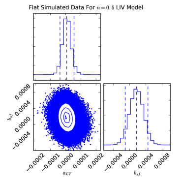
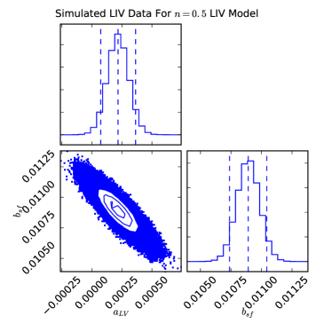
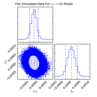
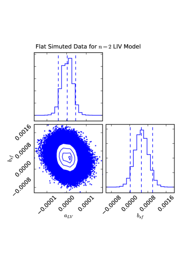
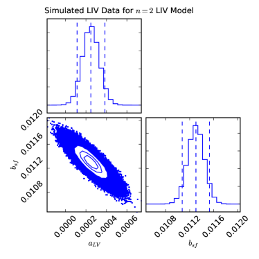
The luminosity distance data and the time delay data have redshift matching problem. For our LIV test, based on the GRB luminosity data and Gaussian distribution, we simulate both non-LIV (Flat Simulated Data) and LIV (Simulated LIV Data) time delay data. For Flat Simulated Data, the priors are set to $a_{LV}=0\pm 0.001$, $b_{sf}=0\pm 0.001$. For Simulated LIV Data, the priors are set to $a_{LV}=0.001\pm 0.0001$, $b_{sf}=0.001\pm 0.0001$. The purpose of the two simulations is to test the validity of the CMITD method. Then the simulated priors of $a_{LV}$ and $b_{sf}$ are assumed as small ones.

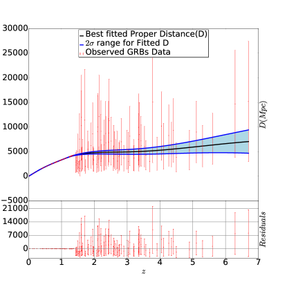
We use GAPP which is a Gaussian Process (GP) module written by python [33] to do the non-linear regression for proper distance. And we pick out the one have the same redshift with the true time delay data. We tried to do GP on the true time delay as well. As the number of time delay data is limited, its best-fitted line is zero. The GP on time delay data gives a too strong prior. Therefore, we only do GP on the luminosity data. To supplement the details, we plot the $D$ residuals in Figure 1 which give an increasing curve of $D$ and consist with expanding universe scenario. Increasing $D$ satisfies the condition of Mean Value Theorem of Integrals.

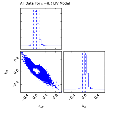
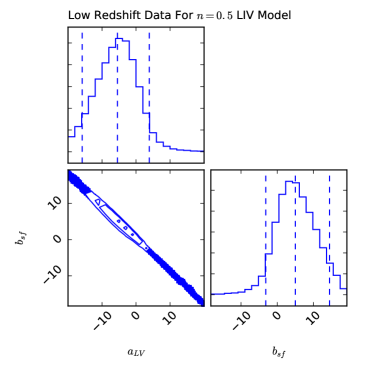
As the luminosity distance data in the range $z<1.4$ are calibrated by the Union2.1 data [32], the error of low redshift $D$ are much smaller than that of the high redshift ones which are calibrated from the $z<1.4$ redshift data [32]. To see the effect of different errors, we choose the data in $z\leq 6.29$ range as All Data and the data in $z\leq 1.4$ range as Low Redshift Data. And to search the error effect of $X$, we remove the $X$ error by hand and call this dataset as "$X$ error Removed Data". We summarize the five kinds of data in Table 1.

Data Sets	$X$	$Y$	Prior
Flat Simulated Data	True	Simulated	$a_{LV}=0\pm 0.001$, $b_{sf}=0\pm 0.001$
Simulated LIV Data	True	Simulated	$a_{LV}=0.001\pm 0.0001$, $b_{sf}=0.001\pm 0.0001$
All Data	GP	True	$-$
Low Redshift Data	GP	True	$z<1.4$
$X$ Error Removed Data	GP	True	Remove X error by hand

Table 1: The five different Data Sets. GP and Simulation make the redshifts of X (luminosity distance data) and Y (time delay data) matched.

Figure 1: The red data points on the top are the proper Distance $D$ derived from GRBs luminosity distance data with its residual in the below panel. The blue region are the $95\%$ C.L. range of GP and the red line is the best fitted line of GP.

Models	Flat Simulated Data	Simulated LIV Data
$n=0.5$	$a_{LV}=0.000007_{-0.000027-0.000055}^{+0.000027+0.000058}$	$a_{LV}=0.00022_{-0.00009-0.00018}^{+0.00009+0.00017}$
	$b_{sf}=0.00017_{-0.00017-0.00033}^{+0.00017+0.00033}$	$b_{sf}=0.01089_{-0.00009-0.00014}^{+0.00009+0.00016}$
$n=1$	$a_{LV}=0.000007_{-0.000028-0.000054}^{+0.000025+0.000053}$	$a_{LV}=0.00018_{-0.00008-0.00017}^{+0.00009+0.00017}$
	$b_{sf}=0.00023_{-0.00020-0.00039}^{+0.00020+0.00039}$	$b_{sf}=0.01107_{-0.00011-0.00021}^{+0.0.00011+0.00021}$
$n=2$	$a_{LV}=0.000003_{-0.000029-0.000054}^{+0.000026+0.000054}$	$a_{LV}=0.00025_{-0.00008-0.00017}^{+0.00008+0.00016}$
	$b_{sf}=0.00052_{-0.00030-0.00058}^{+0.00030+0.00058}$	$b_{sf}=0.01130_{-0.00014-0.00028}^{+0.00014+0.00028}$

Table 2: Mean and $2\sigma$ values for $a_{LV}$ and $b_{sf}$ for Flat Simulated Data and Simulated LIV data.

Models	All Data	Low Redshfit Data	$X$ error Removed Data
$n=0.5$	$a_{LV}=0.0548_{-0.0681-0.1531}^{+0.0757+0.1611}$	$a_{LV}=-5.6142_{-6.4311-12.5395}^{+5.6421+10.7426}$	$a_{LV}=0.2609_{-0.1468-0.2887}^{+0.1466+0.2889}$
	$b_{sf}=0.0332_{-0.0504-0.1122}^{+0.0485+0.1055}$	$b_{sf}=5.2039_{-4.9938-9.4253}^{+5.8457+11.3596}$	$b_{sf}=-0.0714_{-0.0750-0.1477}^{+0.0752+0.1481}$
$n=1$	$a_{LV}=0.0154_{-0.1055-0.1479}^{+0.0557+0.1260}$	$a_{LV}=6.6345_{-13.2444-19.4092}^{+9.4344+12.4488}$	$a_{LV}=0.0978_{-0.1108-0.2167}^{+0.1106+0.2196}$
	$b_{sf}=0.1148_{-0.0650-0.1536}^{+0.1050+0.1958}$	$b_{sf}=-6.5102_{-10.4932-13.4898}^{+14.8697+21.4869}$	$b_{sf}=-0.0033_{-0.1035-0.2045}^{+0.1035+0.2035}$
$n=2$	$a_{LV}=0.0025_{-0.0168-0.0273}^{+0.0115+0.0247}$	$a_{LV}=0.0616_{-0.3350-0.8864}^{+0.4237+1.0175}$	$a_{LV}=0.0187_{-0.0170-0.0335}^{+0.0170+0.0333}$
	$b_{sf}=-0.0310_{-0.0554-0.1169}^{+0.0604+0.1252}$	$b_{sf}=0.0678_{-1.0007-2.1588}^{+0.8382+2.0100}$	$b_{sf}=-0.1069_{-0.0775-0.1543}^{+0.0776+0.1515}$

Table 3: Mean and $2\sigma$ values for $a_{LV}$ and $b_{sf}$ for All Data, Low Redshift Data and $X$ Error Removed Data.

Figure 2: The constraining results of $n=0.5$ LIV model. Probability distributions with the $1\sigma$ to $2\sigma$ contours corresponding to the parameter $a_{LV}$ and $b_{sf}$ are presented. The panels are for Flat Simulated Data and Simulated LIV Data.

Figure 3: Same as Figure 2, but for All Data and Low Redshift Data separately.

4 Results and Discussion

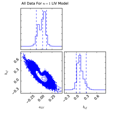
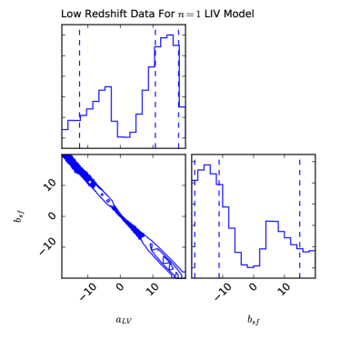
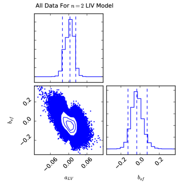
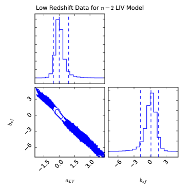
Based on our five data sets, we calculate the relative value of $K$ by Mean Value Theorem for Integrals and fix $H_{0}=67.8km/s/Mpc$ following Planck experiment’s suggestion [31]. PyMC and Deming regression are used to get the propagation and intrinsic value of $a_{LV}$ and $b_{sf}$. We run the MCMC chains $20000000$ steps and present the marginalized distribution for parameters which is a 2-dimensional histogram and list $1\sigma$ and $2\sigma$ constraining ranges of $a_{LV}$ and $b_{sf}$ in Tables 2 and 3. Our corner plots [38] in Figures 2 and 3 show the marginalized distributions of $a_{LV}$ and $b_{sf}$.

4.1 Results from the Simulated Data

Once defining the measurement errors correctly, the Deming regression procedure provides an unbiased estimate of the slope [35]. As Figure 2 and Table 2 show, the results of Flat Simulated Data present that $a_{LV}=0$ and $b_{sf}=0$ are in $1\sigma$ range. And, through our prior precision is assumed as $0.001$, the results reach to $0.00001$ for $a_{LV}$ and $0.0001$ for $b_{sf}$ which is much tighter. For the Simulated LIV Data, the LIV slope $a_{LV}$ and the intrinsic time-lag $b_{sf}$ are negative correlated. And $a_{LV}\neq 0$ and $b_{sf}\neq 0$ are in $2\sigma$ range. Through our prior precision is assumed as $0.0001$, its results reach to $0.0001$ for $a_{LV}$ and $0.0001$ for $b_{sf}$. The results is tighter than the prior of $a_{LV}$ and looser than that of $b_{sf}$. Both results from the simulated data are consistent with the priors.

The parameters $a_{LV}$ and $b_{sf}$ are the propagation and intrinsic effects, their posteriors should be Gaussian distribution. And, regression models work well with symmetrical and bell-shaped curves. As Figure 2 and Table 2 show, the marginalized distributions in simulated data are symmetrical bell-shaped curve. The results consist with the Gaussian distribution theory assumption. By comparing the priors and results for the two simulated data, the conclusion is that we could get the correct LIV results by our effective CMITD method.

4.2 Results form the True Data

As Figure 3 and Table 3 show, All Data give symmetrical and bell-shaped curves for $n=0.5$,$n=1$,$n=2$ LIV models. The luminosity and time delay data from GRBs could separate the propagation effect $a_{LV}$ from the intrinsic source effect $b_{sf}$. The best fitted $a_{LV}$ and $b_{sf}$ are around $0$. Especially, the $1\sigma$ ranges contain the Lorentz invariance value $a_{LV}=0$.

And, the Low Redshift Data do not present good results of LIV because the marginalized distributions of parameters are not symmetrical bell-shaped curves. The $1\sigma$ (or $2\sigma$) ranges of Low Redshift Data cover the $1\sigma$ (or $2\sigma$) ranges of All Data whose results are preciser. Moreover, the $n=1$ model whose results has two peaks does not consist with the Low Redshift Data. As All Data include not only the Low Redshift Data but also high redshift data where $z>1.4$, the CMITD method needs high redshift data. Then, the cosmological-distance-like term $K(z)$ become detectable by accumulating the small LIV effect over a long particle travel time.

If we remove the error of $X$ by hand, the ranges of $a_{LV}$ and $b_{sf}$ are more symmetric but larger than the ones from All Data as Table 3 shows. However, when $n=0.5$ and $n=2$, $a_{LV}=0$ is not in the $1\sigma$ range for $X$ Error Removed Data while $a_{LV}=0$ is in $1\sigma$ range for All Data. It is the main difference between All Data and $X$ Error Removed Data which means removing $X$ error by hand makes the constraining results biased. As calculating $K$ from cosmological model is degenerated to Removing $X$ error by hand, the LIV test results derived from cosmological model are biased as well.

$s_{\pm}$	$n=0.5$	$n=1$	$n=2$
$+1$	$E_{LV}\geq 8.00\times 10^{32}GeV$	$E_{LV}\geq 1.03\times 10^{15}GeV$	$E_{LV}\geq 1.31\times 10^{6}GeV$
(Subluminal)	$1-v/c\leq 4.74\times 10^{-19}$	$1-v/c\leq 3.11\times 10^{-19}$	$1-v/c\leq 5.97\times 10^{-20}$
$-1$	$E_{LV}\geq 3.85\times 10^{33}GeV$	$E_{LV}\geq 1.10\times 10^{15}GeV$	$E_{LV}\geq 1.37\times 10^{6}GeV$
(Superluminal)	$1-v/c\geq-2.16\times 10^{-19}$	$1-v/c\geq-2.91\times 10^{-19}$	$1-v/c\geq-5.44\times 10^{-20}$

Table 4: The range of $E_{LV}$ and velocity by considering $E_{h^{*}}=320keV$, $E_{l^{*}}=25keV$ [12] and the lower limit of $95\%$ confedence level of $a_{LV}$.

4.3 Discussions

Through our CMITD method is cosmological model independent, the observational data may be regarded as model dependent. Considering the comparison between Low Redshift Data and All data in the LIV test, we need high redshift data. Therefore, the choices of data for LIV test are restricted.

Our GRB luminosity data in LIV test are based on Amati relation which is challenged by the selection effect [40]. Indeed, most experience relations are in debate, e.g. the Ghirlanda relation has the redshift ambiguity problem at substantially higher redshift [40]. Here, the GRB luminosity data are calibrated by the Union 2.1 Data which are related with $\Lambda$CDM model. Then, it is not totally free from cosmological model. But the Simulated Data which use the true luminosity data could distinguish LIV effect and their constrained $a_{LV}$ and $b_{sf}$ obey Gaussian distributions. In a conclusion, the effect caused by cosmological model in GRB luminosity data is small and the validity of our CMITD method is not affected. In contrast, the true time delay data is cosmological model dependent. Take the $z=0.45$ data for example [41], to estimate the properties of the host galaxy, the authors adopted a standard cosmology with fixed $H_{0}$ and $\Omega_{m0}$. As the time delay data related to the standard cosmology without LIV effect, the test result does not show any LIV signals. The results given by CMITD method consist with data prior.

Through using dark energy model is regarded as losing unknown errors in LIV test, the comparison among various constraining results is still interesting. For $\Lambda$CDM model, Ref.[15] gives $a_{LV}=-0.017^{+0.0717+0.1416}_{-0.0718-0.1415}$ and $b_{sf}=-0.00013^{+0.0154+0.0308}_{-0.0155-0.0305}$ by using the $\chi^{2}$ methods with the GRBs’ time delay data, the cosmic microwave background data from the Planck first year release, the baryon acoustic oscillation data and Union2 type Ia supernovae data. Our results from CMITD method present $a_{LV}=0.0154_{-0.1055-0.1479}^{+0.0557+0.1260}$ and $b_{sf}=0.1148_{-0.0650-0.1536}^{+0.1050+0.1958}$ by only using the GRBs’ time delay and luminosity distance data. We get a comparable result with the $\Lambda$CDM case in Ref.[15] by using less observational data and no cosmological model. The $1\sigma$ and $2\sigma$ ranges of $a_{LV}$ are at the same order as the results derived from$\Lambda$CDM cosmological model, and the $1\sigma$ and $2\sigma$ ranges of of $b_{sf}$ are one order larger than that derived from $\Lambda$CDM cosmological model.

And, we list the LIV energy scale $E_{LV}$ in Table 4. The parameter $n$ affects the LIV energy scale heavily. The smaller $n$ is, the larger the LIV energy scale is. The $E_{LV}$ parameter is larger than $10^{32}GeV$, $10^{15}GeV$ and $10^{6}GeV$ for $n=0.5$, $n=1$, $n=2$ separately. The LIV energy scale of $n=0.5$ model is much larger than the Planck scale $E_{pl}=\sqrt{\hbar c^{5}/G}=1.2\times 10^{19}GeV$. As the choice of $n$ in Multifractal Spacetime could be in the range of $0<n<1$, if the energy scale of LIV was around Planck scale, the Multifractal Spacetime Theory should choose $n>0.5$. As $E_{LV}$ is too small to be effective, the $n=2$ LIV model need more data break the degeneration between $E_{LV}$ and $n$. The velocity constraints from photon $|1-v/c|$ are at $10^{-19}-10^{-20}$ order. It is also possible that Lorentz violation manifest itself in the gravitational sector. As the observation of the Gravitational Waves (GWs) from the neutron star binary coalescence GW170817 and of the associated Gamma-ray burst GRB 170817A [39] gives $-3\times 10^{-15}<v/v_{GW}-1<7\times 10^{-16}$, the photon part are preciser than the present GWs observation.

5 Conclusion

General Relativity and Lorentz invariance violation are two contradictory theories. As LIV effect depends on $n$ and dark energy model depends GR, unknown systematic errors are given when using dark energy model in LIV tests. In this paper, we proposed a cosmological model independent time delay method to test the Lorentz invariance violation. Five different kinds of Data combinations are used. The simulated time delay data show the method is effective to detect LIV. The true time delay data present non-LIV results because of the data assumption. By comparing the results from Low Redshift Data and All Data, we conclude that high redshift data are needed of LIV test. By comparing the results from All data and $X$ Error Removed Data, we conclude that the error of $X$ is critical for the existence and magnitude of LIV. If the future detections give out model-independent time delay data, more essence of physics could be extracted.

References

- [1] D. Mattingly, Living Rev. Rel. 8, 5 (2005) doi:10.12942/lrr-2005-5 [gr-qc/0502097].
- [2] S. Liberati, Class. Quant. Grav. 30, 133001 (2013) doi:10.1088/0264-9381/30/13/133001 [arXiv:1304.5795 [gr-qc]].
- [3] G. Amelino-Camelia, J. R. Ellis, N. E. Mavromatos, D. V. Nanopoulos and S. Sarkar, Nature 393, 763 (1998) doi:10.1038/31647 [astro-ph/9712103].
- [4] J. Ellis and N. E. Mavromatos, Astropart. Phys. 43, 50 (2013) doi:10.1016/j.astropartphys.2012.05.004 [arXiv:1111.1178 [astro-ph.HE]].
- [5] G. Amelino-Camelia and T. Piran, Phys. Rev. D 64, 036005 (2001) doi:10.1103/PhysRevD.64.036005 [astro-ph/0008107].
- [6] T. Piran, Lect. Notes Phys. 669, 351 (2005) [astro-ph/0407462].
- [7] C. Pfeifer, Phys. Lett. B 780, 246 (2018) doi:10.1016/j.physletb.2018.03.017 [arXiv:1802.00058 [gr-qc]].
- [8] A. De Angelis, arXiv:1610.08245 [astro-ph.HE].
- [9] M. Rodriguez Martinez and T. Piran, JCAP 0604 (2006) 006 doi:10.1088/1475-7516/2006/04/006 [astro-ph/0601219].
- [10] V. Vasileiou et al., Phys. Rev. D 87, no. 12, 122001 (2013) doi:10.1103/PhysRevD.87.122001 [arXiv:1305.3463 [astro-ph.HE]].
- [11] J. R. Ellis, N. E. Mavromatos, D. V. Nanopoulos and A. S. Sakharov, Astron. Astrophys. 402 (2003) 409 doi:10.1051/0004-6361:20030263 [astro-ph/0210124].
- [12] J. R. Ellis, N. E. Mavromatos, D. V. Nanopoulos, A. S. Sakharov and E. K. G. Sarkisyan, Astropart. Phys. 25 (2006) 402 Erratum: [Astropart. Phys. 29 (2008) 158] doi:10.1016/j.astropartphys.2006.04.001, 10.1016/j.astropartphys.2007.12.003 [arXiv:0712.2781 [astro-ph], astro-ph/0510172].
- [13] X. B. Zou, H. K. Deng, Z. Y. Yin and H. Wei, Phys. Lett. B 776, 284 (2018) doi:10.1016/j.physletb.2017.11.053 [arXiv:1707.06367 [gr-qc]].
- [14] U. Jacob and T. Piran, JCAP 0801 (2008) 031 doi:10.1088/1475-7516/2008/01/031 [arXiv:0712.2170 [astro-ph]].
- [15] Y. Pan, Y. Gong, S. Cao, H. Gao and Z. H. Zhu, Astrophys. J. 808, no. 1, 78 (2015) doi:10.1088/0004-637X/808/1/78 [arXiv:1505.06563 [astro-ph.CO]].
- [16] S. Weinberg, Gravitation and Cosmology: Principles and Applications of The General Theory of Relativity, John Wiley. Press, New York, 1972.
- [17] N. Yunes, K. Yagi and F. Pretorius, Phys. Rev. D 94 (2016) no.8, 084002 doi:10.1103/PhysRevD.94.084002 [arXiv:1603.08955 [gr-qc]].
- [18] G. Calcagni, Phys. Rev. Lett. 104, 251301 (2010) doi:10.1103/PhysRevLett.104.251301 [arXiv:0912.3142 [hep-th]].
- [19] G. Calcagni, Adv. Theor. Math. Phys. 16, no. 2, 549 (2012) doi:10.4310/ATMP.2012.v16.n2.a5 [arXiv:1106.5787 [hep-th]].
- [20] G. Calcagni, JHEP 1201, 065 (2012) doi:10.1007/JHEP01(2012)065 [arXiv:1107.5041 [hep-th]].
- [21] G. Calcagni, Eur. Phys. J. C 77, no. 5, 291 (2017) doi:10.1140/epjc/s10052-017-4841-6 [arXiv:1603.03046 [gr-qc]].
- [22] G. Amelino-Camelia, Phys. Lett. B 510, 255 (2001) doi:10.1016/S0370-2693(01)00506-8 [hep-th/0012238].
- [23] J. Magueijo and L. Smolin, Phys. Rev. Lett. 88, 190403 (2002) doi:10.1103/PhysRevLett.88.190403 [hep-th/0112090].
- [24] G. Amelino-Camelia, Nature 418, 34 (2002) doi:10.1038/418034a [gr-qc/0207049].
- [25] G. Amelino-Camelia, Symmetry 2, 230 (2010) [arXiv:1003.3942 [gr-qc]].
- [26] A. S. Sefiedgar, K. Nozari and H. R. Sepangi, Phys. Lett. B 696, 119 (2011) doi:10.1016/j.physletb.2010.11.067 [arXiv:1012.1406 [gr-qc]].
- [27] P. Horava, JHEP 0903, 020 (2009) doi:10.1088/1126-6708/2009/03/020 [arXiv:0812.4287 [hep-th]].
- [28] P. Horava, Phys. Rev. D 79, 084008 (2009) doi:10.1103/PhysRevD.79.084008 [arXiv:0901.3775 [hep-th]].
- [29] S. I. Vacaru, Gen. Rel. Grav. 44, 1015 (2012) doi:10.1007/s10714-011-1324-1 [arXiv:1010.5457 [math-ph]].
- [30] D. Blas and H. Sanctuary, Phys. Rev. D 84, 064004 (2011) doi:10.1103/PhysRevD.84.064004 [arXiv:1105.5149 [gr-qc]].
- [31] P. A. R. Ade et al. [Planck Collaboration], Astron. Astrophys. 594, A13 (2016) doi:10.1051/0004-6361/201525830 [arXiv:1502.01589 [astro-ph.CO]].
- [32] J. Liu and H. Wei, Gen. Rel. Grav. 47, no. 11, 141 (2015) doi:10.1007/s10714-015-1986-1 [arXiv:1410.3960 [astro-ph.CO]].
- [33] M. Seikel, C. Clarkson and M. Smith, JCAP 1206 (2012) 036 [arXiv:1204.2832 [astro-ph.CO]].
- [34] Deming, W. E. (1943). Statistical adjustment of data. Wiley, NY (Dover Publications edition, 1985). ISBN 0-486-64685-8.
- [35] Kristian Linnet, Performance of Deming regression analysis in case of misspecified analytical error ratio in method comparison studies, Clinical Chemistry, 44:5 1024-1031 (1998).
- [36] L. Bonetti, L. R. d. S. Filho, J. A. Helay?l-Neto and A. D. A. M. Spallicci, arXiv:1709.04995 [hep-th].
- [37] Patil, David Huard, Christopher J.Fonnesbeck J.Stat Softw.2010 Jul:35(4):1-81
- [38] Daniel Foreman-Mackey, corner.py: Scatterplot matrices in Python,The Journal of Open Source Software, 2016,24
- [39] B. P. Abbott et al. [LIGO Scientific and Virgo and Fermi-GBM and INTEGRAL Collaborations], Astrophys. J. 848, no. 2, L13 (2017) doi:10.3847/2041-8213/aa920c [arXiv:1710.05834 [astro-ph.HE]].
- [40] A. C. Collazzi, B. E. Schaefer, A. Goldstein and R. D. Preece, Astrophys. J. 747, 39 (2012) doi:10.1088/0004-637X/747/1/39 [arXiv:1112.4347 [astro-ph.HE]].
- [41] P. A. Price et al., AIP Conf. Proc. 662, 56 (2003) doi:10.1063/1.1579299 [astro-ph/0201399].