A Generic Self-Evolving Neuro-Fuzzy Controller based High-performance Hexacopter Altitude Control System

Abstract

Nowadays, the application of fully autonomous system like rotary wing unmanned air vehicles (UAVs) is increasing sharply. Due to the complex nonlinear dynamics a huge research interest is witnessed in developing learning machine based intelligent, self-organizing evolving controller for these vehicles notably to address the system’s dynamic characteristics. In this work, such an evolving controller namely Generic-controller (G-controller) is proposed to control the altitude of a rotary wing UAV namely hexacopter. This controller can work with very minor expert domain knowledge. The evolving architecture of this controller is based on an advanced incremental learning algorithm namely Generic Evolving Neuro-Fuzzy Inference System (GENEFIS). The controller does not require any offline training, since it starts operating from scratch with an empty set of fuzzy rules, and then add or delete rules on demand. The adaptation laws for the consequent parameters are derived from the sliding mode control (SMC) theory. The Lyapunov theory is used to guarantee the stability of the proposed controller. In addition, an auxiliary robustifying control term is implemented to obtain a uniform asymptotic convergence of tracking error to zero. Finally, the G-controller’s performance evaluation is observed through the altitude tracking of a UAV namely hexacopter for various trajectories.

I Introduction

Unmanned air vehicles (UAVs) are aircraft with no pilot on board. UAV’s autonomy shifts from partial to complete, which starts from the human operator based partial remote control to completely self-governing control by onboard computers. Autonomy empowers UAVs to perform some tasks very well where human contribution would be hazardous, or too tedious. In addition, due to their light weight, fuel efficiency and easier maintenance than their manned counterparts, they are getting prevalence day by day with huge applicability in both military and civil sectors [1]. In connection to the wing types, UAVs are normally characterized into three subdivisions, and they are namely: 1) fixed wing, 2) rotary wing, and 3) flapping wing. The rotary wing UAVs (RUAVs) can be additionally categorized by the number of rotors like a helicopter, quadcopter, hexacopter, octocopter, and so forth.

Designing high-performance flight control systems for a UAV is a critical and challenging task [2]. There are some important considerations in designing a reliable flight control system. The first challenge is related to the robustness of the closed loop control in the face of uncertainties, such as unpredictable external airflows (e.g. severe wind gusts) and modelling error. The motion of a small UAV can be highly vulnerable to the adverse impacts of wind gusts that can force the system to depart from its desired trajectory. This phenomena can lead to significant overshoots and tracking offsets, which are undesirable in light of safety and efficiency issues. Significant variations in plant dynamics (e.g. due to payload changes) can seriously deteriorate the performance of fixed-gain control systems [3]. To overcome this problem, a high-degree of flight autonomy is required through the availability of robust and adaptive flight control systems. It should be pointed out that one major problem with model-based control systems is their dependency on the accuracy of the assumed mathematical model of the system. In practice, there is no perfect mathematical model to capture the whole dynamics of any systems, even for the simplest ones. Although researchers have developed cutting-edge model-based robust controls [4], the performance of linear time-invariant (LTI) robust controls (e.g. H infinity and mu-synthesis[5]) can deteriorate in the face of large uncertainties such as the failure or substantial degradation of servos, control surfaces and sensors.

In such circumstances, approaches without the necessity of accurate mathematical models of the system under control, are much appreciated. Being a model-free approach, the Neural Network (NN) and Fuzzy Logic system (FLS) based controllers have been successfully implemented in many control applications [6, 7, 8] over the past few years. To handle uncertainties in control system, researchers have tried to combine the FLS, NN, FNN system with sliding mode control (SMC), H$\infty$ control, back-stepping, etc. Such amalgamation empowers the FLS, NN, FNN controller with the feature of tuning parameters, which provides a more robust and adaptive control structure. However, such adaptive FNN control structures are not able to evolve their structures by adding or pruning rules. It forces the controller to determine the number of rules a priori, where a selection of few fuzzy rules may hinder to achieve adequate and desired control performance. On the other hand, consideration of too many rules usually create complex structures, which make them impossible to employ in real time. A solution to the problem is utilization of evolving structure through the addition or deletion of rules.

In recent time, researchers are trying to develop evolving FLS, NN, FNN controllers by employing various approaches to add or delete the rules [9, 10, 11, 12, 13, 14]. In these controllers, the consequents are adapted using gradient-based algorithms, evolutionary algorithms, or SMC theory. In case of gradient-based algorithms slow convergence speed may be witnessed, in evolutionary algorithm based controllers the stability proof is difficult and questionable [15], and SMC theory based adaptation methods, there exists a dependency on PID parameters [16]. To overcome these limitations, a new evolving controller namely Generic-controller (G-controller) is proposed in our work, where the evolving architecture is developed using an incremental learning method called GENEFIS [17], and the consequents are adapted using SMC theory without any dependency on the PID gains. Furthermore, the integration of GART+ in evolving rules triggers a quick response, and a reduction in computational complexity due to the unnecessary pruned rules. Utilization of self-organizing sliding parameters is a newly used concept and contribution of our work too.

The organization of the remaining part of the paper is as follows: In Section II, the formulation of the hexacopter air vehicle, existing challenges in its control methods are discussed. Section III describes the self-organizing mechanism of the G-controller. In the next section IV, the SMC theory based adaptation of the consequent parameters are explained. The performance of the proposed controller is summarized, compared and discussed in section V. At last, the paper ends with the concluding remarks mentioned in Section VI.

II Problem Formulation in Unmanned Hexacopter Air Vehicle

The simulated hexacopter plant is developed by UAV laboratory of the UNSW at the Australian Defence Force Academy. The model is of medium fidelity and contains both full 6 degrees of freedom (DOF) rigid body dynamics and non-linear aerodynamics. The hexacopter simulated plant introduces two extra degrees of freedom which are obtained by shifting two masses using two aircraft servos with each mass sliding along its own rail aligned in longitudinal and lateral directions respectively, which makes the plant an over-actuated system. The top-level diagram of this over-actuated simulated plant is exhibited in Fig. 1. The mathematical modelling of the hexcopter along with problem formulation is described in the following paragraphs of this section.

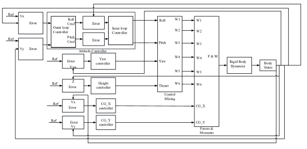
Figure 1: Top-level diagram of the over-actuated simulated Hexacopter plant (adapted from [18] with proper permission)

The body axes system of the hexacopter Unmanned Aerial Vehicle (UAV) are fixed to the aircraft center of gravity and rotates as the aircraft’s attitude changes. This set of axes is particularly useful as the sensors are fixed with respect to the body axes. Another set of axes, known as the inertial axes, are required for navigation and defined with respect to the surface of the earth. The inertial axes are aligned so that the x-axis is horizontal and points North, the y-axis is horizontal and points East and the z-axis is positive down towards the center of the earth. A precise mapping between the inertial and body axes can be made based on the attitude of the hexacopter.

Using standard aircraft nomenclature, the velocity components of the hexacopter along the body axes x, y and z are given the designations $u$, $v$ and $w$ respectively. Likewise, the body axes rotation rates of the hexacopter are $p$, $q$ and $r$. The sense of the rotations are defined in accordance with a right hand axes system. In order to properly define the orientation of an aircraft it is not only necessary to define a coordinate system about which to apply rotations, but also the order in which they are applied. In aviation three Euler angles are used to describe the orientation of an aircraft with respect to an axes system fixed to the earth. These angles use the familiar designations roll($\phi$), pitch($\theta$) and yaw($\psi$). In order to avoid the wraparound problem and to linearise the attitude update, the hexacopter model makes use of the four quaternion parameters $q_{i}$ (where $i=0,1,2,3$) to store attitude and are converted to the Euler angles as required using Eq. 1.

$$\begin{array}[]{ccc}q_{0}&=&\cos\frac{\phi}{2}\cos\frac{\theta}{2}\cos\frac{\psi}{2}+\sin\frac{\phi}{2}\sin\frac{\theta}{2}\sin\frac{\psi}{2}\\ q_{1}&=&\sin\frac{\phi}{2}\cos\frac{\theta}{2}\cos\frac{\psi}{2}-\cos\frac{\phi}{2}\sin\frac{\theta}{2}\sin\frac{\psi}{2}\\ q_{2}&=&\cos\frac{\phi}{2}\sin\frac{\theta}{2}\cos\frac{\psi}{2}+\sin\frac{\phi}{2}\cos\frac{\theta}{2}\sin\frac{\psi}{2}\\ q_{3}&=&\cos\frac{\phi}{2}\cos\frac{\theta}{2}\sin\frac{\psi}{2}-\sin\frac{\phi}{2}\sin\frac{\theta}{2}\cos\frac{\psi}{2}\end{array}$$ (1)

In general flight, rotors of the hexacopter experience a relative freestream velocity due to its own motion of $V_{\infty}$. The airstream is deflected through the actuator disc by speed $V_{i}$ at the disc and can be shown to change the downstream flow by $2V_{i}$. This flow is made up of components $V_{n}$ and $V_{t}$ perpendicular and tangential to each rotor disk respectively. The values of $V_{n}$ and $V_{t}$ are calculated by adding the perpendicular and tangential components of $V_{\infty}$ to the airflow created by pitching, rolling and yawing motions at each rotor. In this modelling it is assumed that the inflow $V_{i}$ does not change with radius or azimuth. The elemental forces are integrated to achieve a closed form solution for thrust in terms of blade pitch ($\theta_{0}$), inflow relative to the rotor disk ($\lambda^{{}^{\prime}}$) and advance ratio ($\mu$) as per Eq. 2 as derived in [19].

$$T=\frac{\rho a(\Omega R)^{2}A_{b}}{2}\left[\frac{1}{3}\theta_{0}\left(1+\frac{3}{2}\mu^{2}\right)-\frac{1}{2}\lambda^{{}^{\prime}}\right]$$ (2)

where $\Omega$ is the blade rotational speed and

$$\lambda^{{}^{\prime}}=\frac{V_{i}+V_{n}}{\Omega R}\;\;\mbox{and}\;\;\mu=\frac{V_{t}}{\Omega R}$$ (3)

Based on the downwash for the equivalent wing, the mean induced velocity $V_{i}$ is expressed as follows:

$$V_{i}=\frac{T}{2\rho A\hat{V}}\;\;\mbox{where}\;\;\hat{V}=\sqrt{V_{T}^{2}+(V_{n}+V_{i})^{2}}$$ (4)

To obtain a good match between our developed hexacopter model and experiments, Eq. 4 is modified in our work as follows:

$$V_{i}^{2}=\sqrt{\left(\frac{\hat{V}}{2}\right)^{2}+\left(\frac{T}{2\rho A}\right)^{2}}-\frac{\hat{V}^{2}}{2}$$ (5)

The yawing torque $N$ generated by each rotor of the hexacopter results from the drag of the rotor blades through the air. The rotor torque is calculated by dividing the main rotor power $P_{tot}$ by the angular velocity as follows

$$N=\frac{P_{tot}}{\Omega}$$ (6)

The power $P_{tot}$ is due to a number of sources: the induced power (Pind) which is the power required to create the induced velocity $V_{i}$ and climb against gravity. And the profile power ($P_{0}$) which is the power to overcome the profile drag of the blades. Therefore, the power $P_{tot}$ is written compactly as follows

$$P_{tot}=P_{ind}+P_{0}$$ (7)

where

$$P_{ind}=k_{ind}TV_{i}+TV_{c}$$ (8)

$$P_{0}=\frac{\sigma C_{D_{0}}}{8}(1+\kappa\mu^{2})$$ (9)

where $k_{ind}$ is a correction factor to compensate for non-uniform induced velocity, tip loss effects etc. Likewise the constant $\kappa$ corrects for skewed flow and other effects in forward flight. $V_{c}$ represents the climb speed of the rotor. For the purposes of this analysis we ignored the effects of vortex ring state in rapid descent.

The body of the hexacopter UAV is assumed to act as a rigid body. Newton’s second law of motion can be used to derive the relationships between the forces and moments acting on the helicopter and the linear and angular accelerations. Assuming that the hexacopter is of a conventional mass distribution, it is usual that the xz plane is a plane of symmetry, so that the cross product moments of inertia $Iyz=Ixy=0$. In this case the equations of motion are those in Eq. 10. A good derivation of these equations are adopted from the flight mechanics text by Nelson [20].

$$\begin{array}[]{ccc}F_{x}&=&m(\dot{u}+qw\text{\textminus}rv)\\ F_{y}&=&m(\dot{v}+ru\text{\textminus}pw)\\ F_{z}&=&m(\dot{w}+pv\text{\textminus}qu)\\ L&=&I_{x}\dot{p}\text{\textminus}I_{xz}\dot{r}+qr(I_{z}\text{\textminus}I_{y})\text{\textminus}I_{xz}pq\\ M&=&I_{y}\dot{q}+rp(I_{x}\text{\textminus}I_{z})+I_{xz}(p^{2}\text{\textminus}r^{2})\\ N&=&\text{\textminus}I_{xz}\dot{p}+I_{z}\dot{r}+pq(I_{y}\text{\textminus}I_{x})+I_{xz}qr\end{array}$$ (10)

where

$$\begin{array}[]{ccc}I_{x}&=&\int\int\int(y^{2}+z^{2})dm\\ I_{y}&=&\int\int\int(x^{2}+z^{2})dm\\ I_{z}&=&\int\int\int(x^{2}+y^{2})dm\\ I_{xy}&=&\int\int\int xydm\\ I_{xz}&=&\int\int\int xzdm\\ I_{yz}&=&\int\int\int yzdm\end{array}$$ (11)

The mass $m$ and mass moments of inertia $Ix,\>Iy,\>Iz$ and $I_{xz}$ of the hexacopter are given in table I.

Table I: Hexacopter inertia properties

Parameter	Description	Units	Value
$m$	mass	$kg$	3.0
$I_{x}$	Mass Moment about x-axis	$kgm^{2}$	0.04
$I_{y}$	Mass Moment about y-axis	$kgm^{2}$	0.04
$I_{z}$	Mass Moment about z-axis	$kgm^{2}$	0.06
$I_{xz}$	Product of Inertia	$kgm^{2}$	0
$g$	Gravitational constant	$ms^{-2}$	9.81

For robustness, the attitude of the hexacopter is stored as a quaternion and updated using the following Eq. 12 provided in [21]. The quaternion attitude update also removes the need to use trigonometric functions which would be required if integrating the Euler angle differential equations.

$$\left[\begin{array}[]{c}q_{0}\\ q_{1}\\ q_{2}\\ q_{3}\end{array}\right]=-\frac{1}{2}\left[\begin{array}[]{cccc}0&p&q&r\\ -p&0&-r&q\\ -q&r&0&-p\\ -r&-q&p&0\end{array}\right]$$ (12)

The final step in updating the rigid body states is to update the position of the hexacopter in global coordinates relative to an earth-based axes system. The local velocities $u$, $v$ and $w$ are first converted to global velocities $\dot{X}$ , $\dot{Y}$ and $\dot{Z}$ by multiplying the local velocities by the rotation matrix $B$ as in Eq. 13. The rotation matrix can be determined directly from the quaternions using Eq. 14. These velocities are then integrated to obtain the global position $[X,\>Y,\>Z]$.

$$\begin{array}[]{ccc}\left[\begin{array}[]{c}\dot{X}\\ \dot{Y}\\ \dot{Z}\end{array}\right]&=&B\left[\begin{array}[]{c}u\\ v\\ w\end{array}\right]\end{array}$$ (13)

where

$$\begin{array}[]{lcc}B=\\ \left[\begin{array}[]{ccc}q_{0}^{2}+q_{1}^{2}\text{-}q_{2}^{2}-q_{3}^{2}&2(q_{1}q_{2}+q_{0}q_{3})&2(q_{1}q_{2}+q_{0}q_{3})\\ 2(q_{1}q_{2}\text{\textminus}q_{0}q_{3})&q_{0}^{2}+q_{1}^{2}\text{-}q_{2}^{2}\text{-}q_{3}^{2}&2(q_{2}q_{3}+q_{0}q_{1})\\ 2(q_{1}q_{3}+q_{1}q_{2})&2(q_{2}q_{3}\text{\textminus}q_{0}q_{1})&q_{0}^{2}-q_{1}^{2}\text{\textminus}q_{2}^{2}+q_{3}^{2}\end{array}\right]\end{array}$$ (14)

Eq. 10 have been implemented as a C code SIMULINK R S-function in the simulated hexacopter plant. The states for the dynamics block are position, local velocity components in the hexacopter axes system, rotation rates and quaternion attitude. Inputs to the block are the forces and moments acting on the hexacopter while the outputs are accelerations, local velocities, position, body angular rates and attitude. From the body states block, the body position of the hexacopter in Z- axes i.e. the altitude $Z$ and attitude (roll and pitch) is supplied to the error calculation block. From here the error is calculated by measuring the difference between actually obtained altitude, attitude and desired reference altitude, attitude. This error is supplied to the proposed G-controller. To prove the closed-loop stability by considering both plants and controller, SMC theory based sliding surface is utilized in this work, where there is no plant parameter dependency. It makes our proposed G-controller a plant parameter free i.e. a real model-free controller.

III Self-organizing Mechanism of G-controller

The G-controller is built using a self-evolving fuzzy system namely GENEFIS [17], where GENEFIS is an evolving TS fuzzy system with ellipsoidal contours in arbitrary positions. a typical fuzzy rule of the G-controller can be presented as follows:

$$\text{IF}\leavevmode\nobreak\ Z\leavevmode\nobreak\ \text{is}\leavevmode\nobreak\ R_{i},\leavevmode\nobreak\ \text{then}\leavevmode\nobreak\ y_{i}=b_{0i}+b_{1i}\zeta_{1}+b_{2i}\zeta_{2}+...+b_{ki}\zeta_{k}$$ (15)

where $R_{i}$ denotes the $i-th$ rule (membership function) constructed from a concatenation of fuzzy sets and epitomizing a multidimensional kernel, $k$ represents the dimension of input feature, $Z$ is an input vector of interest, $b_{i}$ is the consequent parameter, $\zeta_{k}$ is the $k-th$ input feature. The predicted output of the self-evolving model can be expressed as:

$$\hat{y} =\sum\limits_{i=1}^{j}\psi_{i}(\zeta)y_{i}(\zeta)=\frac{\sum\limits_{i=1}^{j}R_{i}y_{i}}{\sum\limits_{i=1}^{j}R_{i}}$$

$$=\frac{\sum_{i=1}^{j}\text{exp}(-(Z-\Theta_{i})\Sigma_{i}^{-1}(Z-\Theta_{i})^{T})y_{i}}{\sum_{i=1}^{j}\text{exp}(-(Z-\Theta_{i})\Sigma_{i}^{-1}(Z-\Theta_{i})^{T})}$$ (16)

In Eq. 16, $\Theta_{i}$ is the centroid of the $i-th$ fuzzy rule $\Theta_{i}\in\Re^{1\times j}$, $\Sigma_{i}$ is a non-diagonal covariance matrix $\Sigma_{i}\in\Re^{k\times k}$ whose diagonal components are expressing the spread of the multivariate Gaussian function, and $k$ is the number of fuzzy rules.

III-A Mechanism of Online Rule-Growing

The Datum Significance (DS) method developed in [22] is extended in [9] to cope with multivariate Gaussian membership function, which is utilized in our work as a rule-growing mechanism. In that regards, after several mathematical amendment to the original DS method, the expression is as follows:

$$D_{sig}=|e_{rn}|\frac{\text{det}(\Sigma_{j+1})^{k}}{\sum_{i=1}^{j+1}\text{det}(\Sigma_{i})^{k}}$$ (17)

When a outlier is obtained far away from the nearest rule, a high value of $D_{sig}$ may obtain from Eq. 17 even with a small value of $e_{rn}$. Besides, the obtained $e_{rn}$ may have a high value in overfitting situation. In such situation, a newly-added rule worsen the situation. As a solution to the above mentioned problems, Eq. 17 needs to be separated.

In our work the rule growing method is activated when the rate of change of $e_{rn}$ is positive, where mean and variance of $e_{rn}$ is updated recursively [23] as follows:

$$\bar{e}_{rn}=\frac{n-1}{n}\bar{e}_{rn-1}+\frac{1}{k}\bar{e}_{rn}$$ (18)

$$\bar{\sigma}_{rn}^{2}=\frac{n-1}{n}\bar{\sigma}_{rn-1}^{2}+\frac{1}{k}(\bar{e}_{rn}-\bar{e}_{rn-1})$$ (19)

When the condition $\bar{e}_{rn}+\bar{\sigma}_{rn}^{2}-(\bar{e}_{rn-1}+\bar{\sigma}_{rn-1}^{2})>0$ is fulfilled, the DS criterion presented in Eq. 17 is simplified here as follows:

$$D_{sig}=\frac{\text{det}(\Sigma_{j+1})^{k}}{\sum_{i=1}^{j+1}\text{det}(\Sigma_{i})^{k}}$$ (20)

When the $D_{sig}$ calculated in Eq. 20 satisfied the condition $D_{sig}\geq g$, the rule base is expanded. Here $g$ is a predefined threshold. The possibility of overfitting phenomenon due to a new rule is omitted by using Eq. 20. Besides, this DS criterion can predict the probable contribution of the datum during its lifetime.

III-B Mechanism of Pruning Rule

Numerous modifications are made in Extended Rule significance (ERS) theory to fit them with the proposed G-controller. By using the $k-$fold numerical integration, the final expression of ERS theory utilized in our work is as follows:

$$E_{inf}^{i}=\sum_{i=1}^{j+1}\eta_{i}\frac{\text{det}(\Sigma_{i})^{k}}{\sum_{i=1}^{j}\text{det}(\Sigma_{i})^{k}}$$ (21)

When $E_{inf}^{i}\leq k_{e}$ i.e. the volume of the $i$th cluster is much lower than the summation of volumes of all cluster, the rule is considered as inconsequential and pruned to protect the rule base evolution from its adverse effect. In this work, $k_{e}$ exhibits a plausible trade-off between compactness and generalization of the rule base. The allocated value for $\delta$ is $\delta=[0.0001,1]$, and $k_{e}=10\%\;\text{of}\;\delta$.

III-C Adaptation of Rule Premise Parameters

Generalized Adaptive Resonance Theory+ (GART+) [24] is used in G-controller as a technique to adapt premise parameters. To relieve from the cluster delamination effect, in GENEFIS based G-controller the size of fuzzy rule are constrained by using GART+, which allows a limited grow or shrink of a category. The procedure and conditions of selecting the winning rule using GART+ has explained briefly in our previous work [18] and in [17].

IV SMC Theory-based Adaptation in G-Controller

In our proposed G-controller, the sliding mode control (SMC) theory is applied to adapt the consequent parameters, which can guarantee the robustness of a system against external perturbations, parameter variations, and unknown uncertainties. Therefore, the SMC theory-based adaptation laws are derived to develop the closed-loop system stability. The zero dynamics of the learning error coordinate [25, 26] is defined as time-varying sliding surface as follows:

$$S_{ssr}(u_{g},u)=u_{ARC}(t)=u_{g}(t)+u(t)$$ (22)

The sliding surface for an over-actuated unmanned aerial vehicle namely hexacopter to be controlled is expressed as:

$$s_{H}=e+\lambda_{1}\dot{e}+\lambda_{2}\int_{0}^{t}e(\tau)d\tau$$ (23)

where, $\lambda_{1}=\frac{\alpha_{2}}{\alpha_{1}},$ $\lambda_{2}=\frac{\alpha_{3}}{\alpha_{1}}$,$\>e$ is the error which is the difference between the actual displacement from the hexacopter plant and desired height. In this work, the sliding parameter $\alpha_{1}$ has initialized with a small value $1\times 10^{-6}$, whereas $\alpha_{2}$ has initialized with $1\times 10^{-6},$ and $\alpha_{3}\thickapprox 0.$ Each of the parameters is then evolved by using different learning rates. These learning rates are set in such a way so that the sliding parameters can achieve the desired value in the shortest possible time to create a stable closed-loop control system. A higher initial value of the sliding parameters is avoided, since it may cause a big overshoot at the beginning of the trajectory. In short, to make our proposed G-controller absolutely model free, these sliding parameters are self-organizing rather than predefined constant values.

The adaptation laws for the consequent parameters of the G-controller are chosen as:

$$\dot{\omega}(t)=-\alpha_{1}G(t)\psi(t)s_{H}(t),\;\;\text{where }\;\omega(0)=\omega_{0}\in\Re^{nR\times 1}$$ (24)

where the term $G(t)$ can be updated recursively as follows:

$$\dot{G}(t)=-G(t)\psi(t)\psi^{T}(t)G(t),\;\;\text{where }\;G(0)=G_{0}\in\Re^{nR\times nR}$$ (25)

where $n$ is the number of inputs to the controller, and $R$ is the number of generated rules. These adaptation laws guarantee a stable closed-loop control system, and explained with the stability proof in [18].

V Results and Discussion

In our work, the self-evolving generic neuro-fuzzy controller namely G-controller is utilized to control a six-rotored UAV namely hexacopter. A variety of altitude trajectory tracking is witnessed to evaluate the controller’s performance. Being an self-organizing evolving controller, the G-controller can evolve both the structure and parameters by adding or pruning the rules like many other evolving controllers discussed in the section I. To understand clearly, one of the rule evolving phenomenon in case of constant altitude is presented graphically in Fig. 2. Nonetheless, the addition of GRAT+, multivariate Gaussian function, SMC learning theory based adaptation laws support it to provide an improved trajectory tracking performance. The controllers are employed to control the thrust of the control-mixing box of the hexacopter plant.

The G-controller’s performance is observed with respect to various reference altitude such as: 1) a constant altitude of 1 meter expressed as $Z_{d}(t)=1$; 2) a triangle wave function with a frequency of 0.1 Hz, and amplitude of 2 m; 3) a sine wave function with a frequency of 0.1 Hz, and amplitude of 2 m; and 4) a step function presented as $Z_{d}(t)=u(t)+u(t-5)$. All these results are compared with a Proportional Integral Derivative (PID) controller. The altitude tracking performance of the proposed controller for various trajectories has been observed in Fig. 3. In all cases, better tracking has been observed from the G-controller than the PID controller. The RMSE, rise time, and settling time has been calculated for all these trajectories and outlined in TABLE II. The lower RMSE is obtained from the proposed G-controller. Besides, the settling time of the G-controller is much lower than the PID, which clearly indicates its improvement over the PID controller.

Table II: Measured RMSE, rising and settling time of various controllers in controlling various altitude of the hexacopter

Hexa-copter movement	Desired trajectory	Maximum amplitude & angle	Measured feature	PID	G-controller
Altitude	Constant amplitude	1 m	RMSE	0.2456	0.2417
			Rise time (sec)	3.2291	1.6112
			Settling time (sec)	7.5112	2.9145
	Step function	2 m	RMSE	0.1535	0.1445
			Rise time (sec)	3.2221	1.6111
			Settling time (sec)	12.1211	3.0100
	Sine wave function	2 m	RMSE	0.3335	0.1283
			Rise time (sec)	4.0200	1.9410
			Settling time (sec)	4.1000	2.0100
	Sawtooth wave function	2 m	RMSE	0.4391	0.3930
			Rise time (sec)	2.5710	1.5420
			Settling time (sec)	3.6120	2.7100

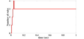
Figure 2: Rule evolving phenomenon of the self-evolving G-controller in case of the constant altitude trajectory of the hexacopter

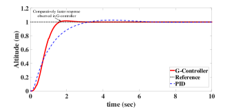
(a)

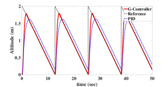
(b)

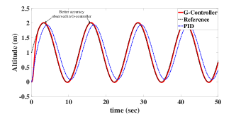
(c)

(d)

Figure 3: Performance observation of a PID and proposed G-controller in tracking various altitude of the hexacopter

VI Conclusion

Being self-organizing and evolving in nature, our proposed G-controller can evolve both the structure and parameters. To increase this controller’s robustness against uncertainties SMC theory based adaptation laws are synthesized too. These are some desirable characteristics to control a highly nonlinear UAV like hexacopter. Therefore, in this work the G-controller based high performance closed-loop altitude control system is developed to track the desired trajectory. In this work, our proposed control algorithm is developed using C programming language considering the compatibility issues to implement directly in hardware of hexacopter and the code is made available online in [27]. The performances are compared with a PID controller and improved results are observed from our proposed G-controller. The controller starts building the structure from scratch with an empty fuzzy set in the closed-loop system. It causes a slow response at the starting point for a very insignificant time, which is a common phenomenon in any self-evolving controller. Nevertheless, the amalgamation of GRAT+, multivariate Gaussian function, SMC learning theory based adaptation laws, the self-evolving mechanism in the G-controller make it faster with a lower computational cost. In addition, the G-controller’s stability is confirmed by both the Lyapunov theory and experiments. In future, the controller will be utilized through hardware-based flight test of various unmanned aerial vehicles.

Acknowlegment

This research is fully supported by NTU start-up grant and MOE Tier-1 grant.

References

- [1] M. M. Ferdaus, S. G. Anavatti, M. A. Garratt, and M. Pratama, “Fuzzy clustering based nonlinear system identification and controller development of pixhawk based quadcopter,” in Advanced Computational Intelligence (ICACI), 2017 Ninth International Conference on. IEEE, 2017, pp. 223–230.
- [2] M. Liu, G. K. Egan, and F. Santoso, “Modeling, autopilot design, and field tuning of a uav with minimum control surfaces,” IEEE Transactions on Control Systems Technology, vol. 23, no. 6, pp. 2353–2360, 2015.
- [3] K. J. Åström and B. Wittenmark, Adaptive control. Courier Corporation, 2013.
- [4] I. R. Petersen, V. A. Ugrinovskii, and A. V. Savkin, Robust Control Design Using H- Methods. Springer Science & Business Media, 2012.
- [5] F. Santoso, M. Liu, and G. K. Egan, “Robust -synthesis loop shaping for altitude flight dynamics of a flying-wing airframe,” Journal of Intelligent & Robotic Systems, vol. 79, no. 2, pp. 259–273, 2015.
- [6] Y. Pan, T. Sun, and H. Yu, “Peaking-free output-feedback adaptive neural control under a nonseparation principle,” IEEE transactions on neural networks and learning systems, vol. 26, no. 12, pp. 3097–3108, 2015.
- [7] Y. Pan and H. Yu, “Biomimetic hybrid feedback feedforward neural-network learning control,” IEEE transactions on neural networks and learning systems, vol. 28, no. 6, pp. 1481–1487, 2017.
- [8] Y. Pan, T. Sun, Y. Liu, and H. Yu, “Composite learning from adaptive backstepping neural network control,” Neural Networks, vol. 95, pp. 134–142, 2017.
- [9] M. Pratama, S. G. Anavatti, P. P. Angelov, and E. Lughofer, “PANFIS: A novel incremental learning machine,” IEEE Transactions on Neural Networks and Learning Systems, vol. 25, no. 1, pp. 55–68, 2014.
- [10] H.-G. Han, X.-L. Wu, and J.-F. Qiao, “Real-time model predictive control using a self-organizing neural network,” IEEE Transactions on Neural Networks and Learning Systems, vol. 24, no. 9, pp. 1425–1436, 2013.
- [11] H. Han and J. Qiao, “Nonlinear model-predictive control for industrial processes: An application to wastewater treatment process,” IEEE Transactions on Industrial Electronics, vol. 61, no. 4, pp. 1970–1982, 2014.
- [12] H.-G. Han, L. Zhang, Y. Hou, and J.-F. Qiao, “Nonlinear model predictive control based on a self-organizing recurrent neural network,” IEEE Transactions on Neural Networks and Learning Systems, vol. 27, no. 2, pp. 402–415, 2016.
- [13] H. Han, W. Zhou, J. Qiao, and G. Feng, “A direct self-constructing neural controller design for a class of nonlinear systems,” IEEE Transactions on Neural Networks and Learning systems, vol. 26, no. 6, pp. 1312–1322, 2015.
- [14] D. Dovžan, S. Blažič, and I. Škrjanc, “Towards evolving fuzzy reference controller,” in Evolving and Adaptive Intelligent Systems (EAIS), 2014 IEEE Conference on. IEEE, 2014, pp. 1–8.
- [15] A. V. Topalov and O. Kaynak, “Online learning in adaptive neurocontrol schemes with a sliding mode algorithm,” IEEE Transactions on Systems, Man, and Cybernetics, Part B (Cybernetics), vol. 31, no. 3, pp. 445–450, 2001.
- [16] E. Kayacan, E. Kayacan, H. Ramon, and W. Saeys, “Adaptive neuro-fuzzy control of a spherical rolling robot using sliding-mode-control-theory-based online learning algorithm,” IEEE Transactions on Cybernetics, vol. 43, no. 1, pp. 170–179, 2013.
- [17] M. Pratama, S. G. Anavatti, and E. Lughofer, “GENEFIS: toward an effective localist network,” IEEE Transactions on Fuzzy Systems, vol. 22, no. 3, pp. 547–562, 2014.
- [18] M. Ferdaus, M. Pratama, S. G. Anavatti, M. A. Garratt, and Y. Pan, “Generic evolving self-organizing neuro-fuzzy control of bio-inspired unmanned aerial vehicles,” arXiv preprint arXiv:1802.00635, 2018.
- [19] J. Seddon, “Basic helicopter aerodynamics. washington, dc, american institute of aeronautics and astronautics,” 1990.
- [20] R. C. Nelson, Flight stability and automatic control. WCB/McGraw Hill New York, 1998, vol. 2.
- [21] B. L. Stevens, F. L. Lewis, and E. N. Johnson, Aircraft control and simulation: dynamics, controls design, and autonomous systems. John Wiley & Sons, 2015.
- [22] G.-B. Huang, P. Saratchandran, and N. Sundararajan, “An efficient sequential learning algorithm for growing and pruning rbf (gap-rbf) networks,” IEEE Transactions on Systems, Man, and Cybernetics, Part B (Cybernetics), vol. 34, no. 6, pp. 2284–2292, 2004.
- [23] P. Angelov, “Fuzzily connected multimodel systems evolving autonomously from data streams,” IEEE Transactions on Systems, Man, and Cybernetics, Part B (Cybernetics), vol. 41, no. 4, pp. 898–910, 2011.
- [24] R. J. Oentaryo, M. J. Er, L. San, L. Zhai, and X. Li, “Bayesian art-based fuzzy inference system: A new approach to prognosis of machining processes,” in Prognostics and Health Management (PHM), 2011 IEEE Conference on. IEEE, 2011, pp. 1–10.
- [25] X. Yu and O. Kaynak, “Sliding-mode control with soft computing: A survey,” IEEE transactions on industrial electronics, vol. 56, no. 9, pp. 3275–3285, 2009.
- [26] E. Kayacan and R. Maslim, “Type-2 fuzzy logic trajectory tracking control of quadrotor vtol aircraft with elliptic membership functions,” IEEE/ASME Transactions on Mechatronics, vol. 22, no. 1, pp. 339–348, 2017.
- [27] M. M. Ferdaus and M. Pratama, “G controller code,” 2018. [Online]. Available: https://www.ntu.edu.sg/home/mpratama/Publication.html