Dictionary Learning and Sparse Coding on Statistical Manifolds

Abstract

In this paper, we propose a novel information theoretic framework for dictionary learning (DL) and sparse coding (SC) on a statistical manifold (the manifold of probability distributions). Unlike the traditional DL and SC framework, our new formulation does not explicitly incorporate any sparsity inducing norm in the cost function being optimized but yet yields sparse codes. Our algorithm approximates the data points on the statistical manifold (which are probability distributions) by the weighted Kullback-Leibeler center/mean (KL-center) of the dictionary atoms. The KL-center is defined as the minimizer of the maximum KL-divergence between itself and members of the set whose center is being sought. Further, we prove that the weighted KL-center is a sparse combination of the dictionary atoms. This result also holds for the case when the KL-divergence is replaced by the well known Hellinger distance. From an applications perspective, we present an extension of the aforementioned framework to the manifold of symmetric positive definite matrices (which can be identified with the manifold of zero mean gaussian distributions), $\mathcal{P}_{n}$. We present experiments involving a variety of dictionary-based reconstruction and classification problems in Computer Vision. Performance of the proposed algorithm is demonstrated by comparing it to several state-of-the-art methods in terms of reconstruction and classification accuracy as well as sparsity of the chosen representation.

1 Introduction

Dictionary learning and sparse coding have found wide applicability in Image/Signal processing, Machine Learning and Computer Vision in recent times. Examples applications include but are not limited to, image classification [33, 37], image restoration [51] and face recognition [50] and many others. The traditional dictionary learning (DL) and sparse coding (SC) formulation assumes that the input data lie in a vector space, and assumes a linear generative model for the data by approximating the data with a sparse linear combination of the dictionary atoms (elements). Thus, the objective function of the DL problem typically has a data fidelity term to minimize the “reconstruction error” in the least squares sense. Sparsity is then enforced on the weights in the linear combination via a tolerance threshold on the $\ell_{0}$-norm of the weight vector. This however leads to an NP-hard problem and the most popular approach for solving this problem (with no convergence guarantees) is the K-SVD based approach [1]. For a fixed dictionary, a convex approximation to the $\ell_{0}$-norm minimization to induce sparsity can be achieved using the $\ell_{1}$-norm constraint on the weight vector [9, 16, 2]. The problem of finding both the optimal dictionary and the sparse-codes however remains to be a hard computational problem in general. For further discussion on this topic and the problem of complete dictionary recovery over a sphere, we refer the readers to [47], where authors provide a provably convergent algorithm.

In many application domains however, the data do not reside in a vector space, instead they reside on a Riemannian manifold such as the Grassmannian [12, 11], the hypersphere [35, 46, 40], the manifold of symmetric positive definite (SPD) matrices [36, 28, 19, 45, 52] and many others. Generalizing the DL & SC problem from the case of vector space inputs to the case when the input data reside on a Riemannian manifold is however difficult because of the nonlinear structure of Riemannian manifolds [52]. One could consider embedding the Riemannian manifold into a Euclidean space, but a problem with this method is that there does not exist a canonical embedding for a general Riemannian manifold. This motivated researchers [52, 23, 45, 29, 53] to generalize the DL and SC problem to Riemannian manifolds. Though the formulation on a Riemannian manifold involves a “reconstruction error” term analogous to the vector space case, defining a sparsity inducing constraint on a manifold is nontrivial and should be done with caution. This is because, a Riemannian manifold lacks “global” vector space structure since it does not have the concept of a global origin. Hence, as argued in [52], one way to impose the sparsity inducing constraint is via an an affine constraint, i.e., the sparsity constraint is over an affine subspace defined by the tangent space at each data point on the manifold. We now briefly review a few representative algorithms for the DL & SC problem on Riemannian manifolds.

A popular solution to the DL problem is to make use of the tangent spaces, which are linear spaces associated with each point on a Riemannian manifold. This approach essentially involves use of linear approximation in the smooth neighborhood of a point. Guo et al. [21] use a Log-Euclidean framework described at length in [5] to achieve a sparse linear representation in the tangent space at the Fréchet mean of the data. Xie et al. [52] developed a general dictionary learning formulation that can be used for data on any Riemannian manifold. In their approach, for the SC problem, authors use the Riemannian Exponential (Exp.) and Logarithm (Log.) maps to define a generative process for each data point involving a sparse combination of the Log.-mapped dictionary atoms residing on the manifold. This sparse combination is then realized on the manifold via the Exp.-map. Their formulation is a direct generalization of the linear sparsity condition with the exception of the origin of the linear space being at the data point. Further, they impose an affine constraint in the form of the weights in the weight vector summing to one. This constraint implies the use of affine subspaces to approximate the data. For fixed weights however, estimating the dictionary atoms is a hard problem and a manifold line search method is used in their approach. In another method involving DL and SC on the manifold of SPD matrices, Cherian et al. [13] proposed an efficient optimization technique to compute the sparse codes. Most recently, authors in [41] introduced a novel nonlinear DL and SC method for histograms residing in a simplex. They use the well known Wasserstein distance along with an entropy regularization [32] to reconstruct the histograms that are Wasserstein barycenter approximations of the given data (histograms). They solve the resulting optimization for both the dictionary atoms and weights using a gradient based technique. Authors point out that using the entropy regularization leads to a convex optimization problem. However, authors did not discuss sparsity of the ensuing Wasserstein barycenter dictionary based representation. Sparsity property is of significant importance in many applications and the focus of our work here is on how to achieve sparsity without explicitly enforcing sparsity inducing constraints.

Several recent works report the use of kernels to accomplish dictionary learning and sparse coding on Riemannian manifolds [22, 29, 23]. In these, the Riemannian manifold is embedded into the Reproducing Kernel Hilbert Space (RKHS). DL and SC problems are then formulated in the RKHS. RKHS is a linear space, and hence it is easier to derive simple and effective solutions for the DL and SC problems. Recently, authors in [18] presented conditions that must be strictly satisfied by geodesic exponential Kernels on general Riemannian manifolds. This important and significant result provides guidelines for designing a kernel based approach for general Riemannian manifolds.

In this work, we present a novel formulation of the DL and SC problems for data residing on a statistical manifold, without explicitly enforcing a sparsity inducing constraint. The proposed formulation circumvents the difficulty of directly defining a sparsity constraint on a Riemannian manifold. Our formulation is based on an information theoretic framework and is shown to yield sparse codes. Further, we extend this framework to the manifold of SPD matrices. Note that SPD matrices can be identified with the space of zero mean Gaussian distributions, which is a statistical manifold. Several experimental results are presented that demonstrate the competitive performance of our proposed algorithm in comparison to the state-of-the-art.

The rest of the paper is organized as follows: in Section 2, we first present the conventional DL and SC problem formulation in vector spaces and motivate the need for a new formulation of the DL and SC problem on Riemannian manifolds. This is followed by a brief summary of relevant mathematical background on statistical manifolds. Following this, we summarize the mathematical results in this paper and then present the details along with our algorithm for the DL and SC problem. In Section 3, we present several experimental results and comparisons to the state-of-the-art. Finally, in Section 4, we draw conclusions.

2 An Information Theoretic Formulation

In the traditional SC problem, a set of data vectors $X=\{\mathbf{x}_{i}\}_{i=1}^{N}\subset\mathbf{R}^{n}$, and a collection of atoms, $A=\{\mathbf{a}_{j}\}_{j=1}^{r}\subset\mathbf{R}^{n}$, are given. The goal is to express each $\mathbf{x}_{i}$ as a sparse linear combination of atoms in $A$. Let, $A$ be the (overcomplete) dictionary matrix of size $n\times r$ whose $i^{th}$ column consists of $\mathbf{a}_{i}$. Let $W=[\mathbf{w}_{1},\cdots,\mathbf{w}_{N}]$ be a $r\times N$ matrix where each $\mathbf{w}_{i}\in\mathbf{R}^{r}$ consists of the coefficients of the sparse linear combination. In the DL and SC problem, the goal is to minimize the following objective function:

$$\min_{A,w_{1},\cdots,w_{n}}\sum_{i=1}^{n}\|x_{i}-Aw_{i}\|^{2}+\mathbf{Sp}(w_{i}),$$ (1)

Here, $\mathbf{Sp}(w_{i})$ denotes the sparsity promoting term, which can be either an $\ell_{0}$ norm or an $\ell_{1}$ norm. Since, in the above optimization problem, both the dictionary $A$ and the coefficient matrix $W$ are unknown, it leads to a hard optimization problem. As this optimization problem is computationally intractable when the sparsity promoting term is an $\ell_{0}$ norm constraint, most existing approaches use a convex relaxation to this objective using an $\ell_{1}$ norm in place of the $\ell_{0}$ norm constraint when performing the sparse coding. Now, instead of the traditional DL & SC setup where data as well as atoms are vector valued, we address the problem when each data point and the atom are probability densities, which are elements of a statistical manifold (see formal definition below). In this paper, we present a novel DL and SC framework for data residing on a statistical manifold. Before delving into the details, we will briefly introduce some pertinent mathematical concepts from Differential Geometry and Statistical Manifolds and refer the reader to [10, 4] for details.

2.1 Statistical Manifolds: Mathematical Preliminaries

Let $\mathcal{M}$ be a smooth ($C^{\infty}$) manifold [10]. We say that $\mathcal{M}$ is $n$-dimensional if $\mathcal{M}$ is locally Euclidean of dimension $n$, i.e., locally diffeomorphic to $\mathbf{R}^{n}$. Equipped with the Levi-Civita connection $\nabla$, the triplet $(M,g,\nabla)$ is called a statistical manifold whenever both $\nabla$ and the dual connection, $\nabla^{*}$ are torsion free [10, 4].

A point on an $n$-dimensional statistical manifold, $\mathfrak{D}$ (from here on, we will use the symbol $\mathfrak{D}$ to denote a statistical manifold unless specifically mentioned otherwise), can be identified with a (smooth) probability distribution function on a measurable topological space $\Omega$, denoted by $P(\mathbf{x};\bm{\theta})$ [48, 4]. Here, each distribution function can be parametrized using $n$ real variables $(\theta_{1},\cdots,\theta_{n})$. So, an open subset $S$ of a statistical manifold, $\mathfrak{D}$, is a collection of the probability distribution functions on $\Omega$. And the chart map is the mapping from $S$ to the parameter space, $\Theta=\{\bm{\theta}\}\subset\mathbf{R}^{n}$. Let $\mu$ be a $\sigma$-finite additive measure defined on a $\sigma$-algebra of subsets of $\Omega$. Let $f(\mathbf{x};\bm{\theta})$ be the density of $P(\mathbf{x};\bm{\theta})$ with respect to the measure $\mu$ and assume the densities to be smooth $(C^{\infty})$ functions. Now, after giving $\mathfrak{D}$ a topological structure, we can define a Riemannian metric as follows. Let $l(\mathbf{x};\bm{\theta})=\log f(\mathbf{x};\bm{\theta})$, then a Riemannian metric, $g$ can be defined as $g_{ij}(\bm{\theta})=E_{\bm{\theta}}\left[\frac{\partial l(\mathbf{x};\bm{\theta})}{\partial\theta_{i}}\frac{\partial l(\mathbf{x};\bm{\theta})}{\partial\theta_{j}}\right]$, where $E_{\bm{\theta}}[\mathbf{y}]$ is the expectation of $\mathbf{y}$ with respect to $\bm{\theta}$. In general, $g=[g_{ij}]$ is symmetric and positive semi-definite. We can make $g$ positive definite by assuming the functions $\{\frac{\partial l(\mathbf{x};\bm{\theta})}{\partial\theta_{i}}\}_{i=1}^{n}$ to be linearly independent. This metric is called the Fisher-Rao metric [38, 3] on $\mathfrak{D}$.

2.2 Summary of the mathematical results

In the next section, we propose an alternative formulation to the DL and SC problem. We first state a few theorems as background material that will be used subsequently. Then, we define the new objective function for the DL and SC problem posed on a statistical manifold in Section 2.3.1. Our key mathematical results are stated in Theorems 2.6 and 2.7, Corollary 2.6.1 and 2.6.2 respectively. Using these results, we show that our DL & SC framework, which does not have an explicit sparsity constraint, yields sparse codes. Then, we extend our DL and SC framework to the manifold of SPD matrices, $\mathcal{P}_{n}$, in Section 2.3.2.

2.3 Detailed mathematical results

Let the manifold of probability densities, hereafter denoted by $\mathfrak{D}$ be the $n$-dimensional statistical manifold, i.e., each point on $\mathfrak{D}$ is a probability density. We will use the following notations in the rest of the paper.

• Let $\mathfrak{G}$ be a dictionary with $r$ atoms $g_{1}$, $\cdots,$ $g_{r}$, where each $g_{i}\in\mathfrak{D}$.

• Let $\mathfrak{F}=\{f_{i}\}_{i=1}^{N}$ $\subset\mathfrak{D}$ be a set of data points.

• And $w_{ij}$ be nonnegative weights corresponding to $i^{th}$ data point and $j^{th}$ atom, $i\in\{1,\cdots,N\}$ and $j\in\{1,\cdots,r\}$.

Note that, here we assume that each density $f$ or $g$ is parameterized by $\bm{\theta}$. There are many ways to measure the discrepancy between probability densities. One can choose an intrinsic metric and the corresponding distance on a statistical manifold to measure this discrepancy, such as the Fisher-Rao metric [38, 3], which however is expensive to compute. In this paper, we choose an extrinsic measure namely the non-negative divergence measure called the Kullback-Leibler (KL) divergence. The KL divergence [14] between two densities $f_{1}$ and $f_{2}$ on $\mathfrak{D}$ is defined by

$$\text{KL}(f_{1},f_{2})=\int f_{1}(x)\log\frac{f_{1}(x)}{f_{2}(x)}dx$$ (2)

The Hessian of KL-divergence is the Fisher-Rao metric defined earlier. In other words, the KL-divergence between two nearby probability densities can be approximated by half of the squared geodesic distance (induced by the Fisher-Rao metric) between them [3]. The KL-divergence is not a distance as it is not symmetric and does not satisfy the triangle inequality. It is a special case of a broader class of divergences called the $f$-divergences as well as of the well known class of Bregman-divergences. We refer the reader to [6, 30] for more details in this context. Given a set of densities $\mathfrak{F}=\{f_{i}\}$, the KL divergence from $\mathfrak{F}$ to a density $f$ can be defined by,

$$\text{KL}(\mathfrak{F},f)=\displaystyle\max_{i}\text{KL}(f_{i},f).$$ (3)

We can define the KL-center of $\mathfrak{F}$, denoted by $f_{m}(\mathfrak{F})$, by

$$f_{m}(\mathfrak{F})=\operatorname*{arg\,min}_{f}\text{KL}(\mathfrak{F},f).$$ (4)

The symmetrized KL divergence, also called the Jensen-Shannon divergence (JSD) [14] between two densities $f_{1}$ and $f_{2}$ is defined by,

$$\text{JSD}(f_{1},f_{2})=\frac{1}{2}\text{KL}(f_{1},f_{2})+\frac{1}{2}\text{KL}(f_{2},f_{1}).$$ (5)

In general, given the set $\mathfrak{F}=\{f_{i}\}$, define a mixture of densities as, $f=\sum_{i}\alpha_{i}f_{i}$, $\sum\alpha_{i}=1$, $\alpha_{i}\geq 0$, $\forall i$. It is evident that the set of $\{\alpha_{i}\}$ forms a simplex, which is denoted here by $\Delta$. Then, the JSD of the set $\mathfrak{F}$ with the mixture weights $\{\alpha_{i}\}$ is defined as,

$$\text{JSD}(\{f_{i}\})=H(\sum_{i}\alpha_{i}f_{i})-\sum_{i}\alpha_{i}H(f_{i}),$$ (6)

where $H(f)=-\int f(x)\log f(x)dx$ is the Shannon entropy of the density $f$. It is easy to see the following Lemma.

Lemma 2.1.

$\text{JSD}(\{f_{i}\})$ is concave in $\{\alpha_{i}\}$ and JSD attains the minimum at an extreme point of the simplex $\Delta$.

Proof.

We refer the reader to [44] for a proof of this Lemma. ∎

In [44], it was shown that one can compute the KL- center of $\mathfrak{F}$, $f_{m}(\mathfrak{F})$, in Equation 4 using the following theorem:

Theorem 2.2.

The KL center of $\mathfrak{F}$, $f_{m}(\mathfrak{F})$, is given by

$$f_{m}(\mathfrak{F}) = \sum_{i}\hat{\alpha}_{i}f_{i}$$

$$\text{where }\hat{\bm{\alpha}} = \operatorname*{arg\,max}_{\bm{\alpha}}\text{JSD}(\{f_{i}\}).$$

Proof.

We refer the reader to [44] for a proof of this theorem. ∎

Observe that, the $\text{KL}(\mathfrak{F},f)$ defined in Eq. 3 has the positive-definiteness property, i.e., $\text{KL}(\mathfrak{F},f)\geq 0$ for any $\mathfrak{F}$ and $f$ and $\text{KL}(\mathfrak{F},f)=0$ if and only if $f\in\mathfrak{F}$. Both of these properties are evident from the definition of the KL divergence between two densities.

Coding theory interpretation: It should be noted that the above result is the same as the well known redundance-capacity theorem of coding theory presented in [20, 15, 39, 2]. The theorem establishes the equivalence of: the minmax excess risk i.e., redundancy for estimating a parameter $\theta$ from a family/class $\Theta$ of sources, the Bayes risk associated with the least favorable prior and the channel capacity when viewing statistical modeling as a communication via a noisy channel. In [2], a stronger result was shown, namely that, the capacity is also a lower bound for “most” sources in the class. The results in [44] however approached this problem from a geometric viewpoint i.e., one of finding barycenters of probability distributions using the KL-divergence as the “distance” measure. Our work presented here takes a similar geometric view point to the problem at hand, namely the DL-SC problem.

Moving on, we now define the $\ell_{p}$ KL divergence, denoted by $\text{KL}_{p}(\mathfrak{F},f)$, $p>0$ as:

$$\text{KL}_{p}(\mathfrak{F},f)=\|\left(\text{KL}(f_{1},f),\cdots,\text{KL}(f_{N},f)\right)^{t}\|_{p}.$$ (7)

where, $\|.\|_{p}$ is the $\ell_{p}$ norm of the vector and $\mathfrak{F}=\{f_{i}\}_{i=1}^{N}$. It is easy to prove the following property of $\text{KL}_{p}(\mathfrak{F},f)$ in the following Lemma.

Lemma 2.3.

$\text{KL}_{p}(\mathfrak{F},f)$ as defined in Eq. 7 is a well-defined statistical divergence for any $p>0$. Furthermore, the KL divergence as defined in Eq. 3 is a special case of $\text{KL}_{p}$ when $p=\infty$.

Without any loss of generality, we will assume $p=1$ and refer $\ell_{1}$ KL-center to be simply the KL-center for the rest of the paper (unless mentioned otherwise). Now, given the set of densities $\mathfrak{F}=\{f_{i}\}_{i=1}^{N}$ and a set of weights $\{\alpha_{i}\}_{i=1}^{N}$, we can define the weighted KL-center, denoted by $f_{m}(\mathfrak{F},\{\alpha_{i}\})$ as follows:

$$f_{m}(\mathfrak{F},\{\alpha_{i}\})=\operatorname*{arg\,min}_{f}\sum_{i}\alpha_{i}\text{KL}(f_{i},f).$$ (8)

We like to point out that it is however easy to see that the $\ell_{\infty}$ KL-center can not be generalized to the corresponding weighted KL center. The above defined weighted KL-center has the following nice property:

Lemma 2.4.

The weighted KL-center as defined in Eq. 8 is a generalization of the KL-center in Eq. 4 (with $p=1$). The KL-center can be obtained from the weighted KL-center by substituting $\alpha_{i}=1/N$, for all $i$.

Theorem 2.5.

Given $\mathfrak{F}$ and $\{\alpha_{i}\}$ as above, $f_{m}(\mathfrak{F},\{\alpha_{i}\})=\sum_{i}\alpha_{i}f_{i}$

Proof.

For simplicity, assume that each $f_{i}$ is discrete and assume that it can take on $k$ discrete values, $x_{1},\cdots,x_{k}$. Then, consider the minimization of $\sum_{i}\text{KL}(f_{i},f)$ with respect to $f$ subject to the constraint that $f$ is a density, i.e., for the discrete case, $\sum_{j}f(x_{j})=1$. By using a Lagrange multiplier $\lambda$, we get,

$$\frac{\partial}{\partial f(x_{j})}\left\{\sum_{i}\alpha_{i}\text{KL}(f_{i},f)+\lambda\left(\sum_{j}f(x_{j})-1\right)\right\} = 0,\>\forall j$$

$$\implies\left(\lambda-\frac{\sum_{i}\alpha_{i}f_{i}(x_{j})}{f(x_{j})}\right) = 0,\>\forall j$$

$$\implies f(x_{j})=\frac{\sum_{i}\alpha_{i}f_{i}(x_{j})}{\lambda},\>\forall j.$$

Now, by taking $\frac{\partial}{\partial\lambda}\left\{\sum_{i}\alpha_{i}\text{KL}(f_{i},f)+\lambda\left(\sum_{j}f(x_{j})-1\right)\right\}$ and equating to $0$, we get $f(x_{j})=\sum_{i}\alpha_{i}f_{i}(x_{j})$, $\forall j$. Thus, $f=\sum_{i}\alpha_{i}f_{i}$. We can easily extend this to the case of continuous $f_{i}$ by replacing summation with integration and obtain a similar result. ∎

2.3.1 DL and SC on a statistical manifold

Now, we will formulate the DL and SC problems on a statistical manifold. The idea is to express each data point, $f_{i}$ as a sparse weighted combination of the dictionary atoms, $\{g_{j}\}$. Given the above hypothesis, our objective function is given by:

$$\displaystyle\operatorname*{arg\,min}_{\mathfrak{G}^{*},W^{*}}\>\>\>\>E =\sum_{i=1}^{N}\text{KL}\left(f_{i},\hat{f}_{i}\right)$$ (9)

subject to $$\>\>\>w_{ij}\geq 0,\forall i,j$$ (10)

$$\sum_{j}w_{ij}=1,\forall i.$$ (11)

where, $\hat{f}_{i}=\sum_{j=1}^{r}w_{ij}g_{j}$, $\forall i$. In the above objective function, $\hat{f}_{i}$ is the minimizer of the weighted KL-center of $\{g_{j}\}_{j=1}^{r}$ with weights $\{w_{ij}\}_{j=1}^{r}$. The constraint $w_{ij}\geq 0$ and $\sum_{j}w_{ij}=1$ is required to make $\hat{f}_{i}$ a probability density. Note that, we can view $\hat{f}_{i}$ as a reconstructed density from the dictionary elements $\{g_{j}\}$ and weights $\{w_{ij}\}$. We will now prove one of our key result namely, that the minimization of the above objective function with respect to $\{w_{ij}\}$ yields a sparse set of weights.

Theorem 2.6.

Let $\mathfrak{G}=\{g_{j}\}$ and $W=[w_{ij}]$ be the solution of the objective function $E$ in Equation 9. Then,

$$\left(\forall j\right),\text{KL}(f_{i},g_{j})\geq r_{i},\text{ where }r_{i}=\sum_{k}w_{ik}\text{KL}(f_{i},g_{j})$$

Proof.

Consider the random variables $X_{1},\cdots,X_{N}$ with the respective densities $f_{1},\cdots,f_{N}$. Since each dictionary element $g_{j}$ is “derived” from $\{f_{i}\}$, hence, we can view each $g_{j}$ to be associated with a random variable $Y_{j}$ such that $Y_{j}=\tilde{g}_{j}\left(\{X_{i}\}\right)$, i.e., $Y_{j}$ is a transformation of random variables $\{X_{i}\}$. We now have,

$$\begin{split}E&=\sum_{i=1}^{N}\text{KL}\left(f_{i},\sum_{j=1}^{r}w_{ij}g_{j}\right)\\ &=\sum_{i=1}^{N}\left[\int\left\{f_{i}(x)\log(f_{i}(x))dx\right\}\right.-\\ &\left.\int\left\{f_{i}(x)\log\left(\sum_{j}w_{ij}g_{j}(x)\right)\right\}dx\right]\end{split}$$

Using Jensen’s inequality we have,

$$\begin{split}E&\leq&\sum_{i=1}^{N}\left[\int\left\{f_{i}(x)\log(f_{i}(x))dx\right\}-\right.\\ &&\left.\int\left\{f_{i}(x)\sum_{j}w_{ij}\log(g_{j}(x))\right\}dx\right]\\ &=&\sum_{i=1}^{N}E_{X_{i}}\left[\log(f_{i})-\sum_{j}w_{ij}\log(g_{j})\right]\end{split}$$

where, $E_{X}[h(X)]$ is the expectation of $h(X)$, where $h(X)$ is a transformation of the random variable $X$. So,

$$E \leq \sum_{i=1}^{N}E_{X_{i}}[\log(f_{i})]-\sum_{i=1}^{N}\sum_{j}w_{ij}E_{X_{i}}[\log(g_{j})]$$

$$= \sum_{i=1}^{N}\sum_{j=1}^{r}w_{ij}E_{X_{i}}[\log(f_{i})]-\sum_{i=1}^{N}\sum_{j=1}^{r}w_{ij}E_{X_{i}}[\log(g_{j})]$$

$$= \sum_{i=1}^{N}\sum_{j}w_{ij}E_{X_{i}}[\log(f_{i})-\log(g_{j})]$$

$$= \sum_{i=1}^{N}\sum_{j}w_{ij}\text{KL}(f_{i},g_{j})$$

So, $E\leq\sum_{i=1}^{N}\sum_{j}w_{ij}\text{KL}(f_{i},g_{j})$. Since, both $E$ and $\sum_{i=1}^{N}\sum_{j}w_{ij}\text{KL}(f_{i},g_{j})$ attain minima at the same value (equal to $0$), we can minimize $\sum_{i=1}^{N}\sum_{j}w_{ij}\text{KL}(f_{i},g_{j})$ instead of $E$. Using a Lagrange multiplier $r_{i}$ for each constraint $\sum_{j}w_{ij}=1$, and $\gamma_{ij}$ for each constraint $w_{ij}\geq 0$, we get the following function

$$\sum_{j}w_{ij}\text{KL}(f_{i},g_{j})+\sum_{i=1}^{N}r_{i}(1-\sum_{j}w_{ij})-\sum_{i,j}\gamma_{ij}w_{ij}$$

We minimize the above objective function and add the KKT conditions

$$\gamma_{ij}w_{ij}=0$$

to get,

$$\text{KL}(f_{i},g_{j})=\left\{\begin{array}[]{lr}r_{i}+\gamma_{ij},&\text{if }w_{ij}=0\\ r_{i},&\text{if }w_{ij}>0\end{array}\right.$$ (14)

As each $\gamma_{ij}\geq 0$, this concludes the proof. ∎

A straightforward Corollary of the above theorem is as follows:

Corollary 2.6.1.

The objective function $E$ is bounded above by $\sum_{i=1}^{N}r_{i}$, i.e., $E\leq\sum_{i=1}^{N}r_{i}$.

Proof.

From Theorem 2.6, we know that, $E\leq\sum_{i=1}^{N}\sum_{j}w_{ij}\text{KL}(f_{i},g_{j})$. From Equation 14, we can now get $\sum_{j}w_{ij}\text{KL}(f_{i},g_{j})=r_{i}$, $\forall i$. Thus the Corollary holds. ∎

Figure 1: Illustrative figure for Theorem 2.7. Blue and brown circles are atoms with non-zero and zero weights respectively.

We can see that the dictionary elements, $g_{j}$, for which the associated weights are positive, are exactly at the same distance $r_{i}$ from the density $f_{i}$. Corollary 2.6.1 implies that solving the objective function in Equation 9 yields a “tight cluster” structure around each $f_{i}$, as minimizing $E$ is equivalent to minimizing each $r_{i}$.

Corollary 2.6.2.

Let, $f_{i}$ be well approximated by a single dictionary element $g_{l}$. Further assume that $g_{l}$ is a convex combination of a set of dictionary atoms, i.e., $g_{l}=\sum_{k=1}^{r_{1}}w_{ij_{k}}g_{j_{k}}$. Without loss of generality (WLOG), assume that $w_{ij_{k}}>0$, $\forall k$. Let, $r_{i}=\text{KL}(f_{i},g_{l})$ and $\hat{r}_{i}=\text{KL}(f_{i},g_{j_{k}})$, $\forall k=1,\cdots,r_{1}$. Then, $r_{i}<\hat{r}_{i}$.

Proof.

Using the hypothesis in Theorem 2.6, we have,

$$r_{i} = \int f_{i}(x)\log(f_{i}(x))dx-\int f_{i}(x)\log(g_{l}(x))dx$$

$$< \left[\int f_{i}(x)\log(f_{i}(x))dx-\int f_{i}(x)\sum_{k=1}^{r_{1}}w_{ij_{k}}\log(g_{j_{k}})dx\right]$$

$$= \sum_{k=1}^{r_{1}}w_{ij_{k}}\text{KL}(f_{i},g_{j_{k}})$$

$$= \hat{r}_{i}$$

Hence, $r_{i}<\hat{r}_{i}$. Using Corollary 2.6.1, we can see that, in order to represent $f_{i}$, the objective function is to minimize $r_{i}$. Thus, using Corollary 2.6.1, we can say that a sparse set of weights, i.e., corresponding to $g_{l}$, is preferable over a set of non-zero weights, i.e., corresponding to a set of $\{g_{j_{k}}\}$. ∎

Now, we will state and prove the second key result namely, a theorem which states that our proposed algorithm yields non-zero number of atoms whose corresponding weights are zero i.e., $k-sparsity$ for some $k>0$.

Theorem 2.7.

Let $\mathfrak{S}_{i}=\left\{w_{ij}|w_{ij}=0\right\}$, then, with probability $1$, the cardinality of $\mathfrak{S}_{i}$, i.e., $|\mathfrak{S}_{i}|>0$, for all $i$.

Proof.

Let $\mu^{*}$ be the probability measure on $\mathfrak{D}$. let $\mathcal{B}(f,r)$ denote a closed ball of radius $r$ centered at $f\in\mathfrak{D}$, we assume that the measure is bounded, i.e., $\exists$ constants, $\kappa_{1}>0$ and $\kappa_{2}>0$ such that, $\left(\kappa_{1}r\right)^{n}\leq\mu^{*}\left(\mathcal{B}(f,r)\right)\leq\left(\kappa_{2}r\right)^{n}$, for all $0<r\leq 1$. Let us assume, $\mathfrak{G}$ is an $\epsilon$-separated set for some $0<\epsilon\leq 1$. Furthermore, assume that $\mathfrak{F}$ has finite variance, i.e., $\exists C$ such that $\forall i,j$, $\text{KL}\left(f_{i},f_{j}\right)\leq C$, we will call this radius $C$ (closed) ball as the data ball. Let the optimum value of $E/N$ be $r^{*}$, i.e., $r^{*}=\max_{i}\text{KL}\left(f_{i},\hat{f}_{i}\right)$ (see Figure 1). Now, for a given $i$, consider $\mathcal{B}\left(f_{i},r^{*}\right)$, from Theorem 2.6, we know that if for some $j$, $w_{ij}>0$, then, $\text{KL}(f_{i},g_{j})=r^{*}$, else, $\text{KL}(f_{i},g_{j})>r^{*}$.

Thus, $\mathfrak{S}_{i}$ can be rewritten as, $\mathfrak{S}_{i}=\left\{g_{j}|\text{KL}(f_{i},g_{j})>r^{*}\right\}$. Let, $N\left(r^{*},C\right)$ be the number of $g_{j}$s in $\mathcal{B}(f_{i},C)\setminus\mathcal{B}(f_{i},r^{*})$. Then, $N\left(r^{*},C\right)$ follows a Poisson distribution with rate $\lambda=\mu^{*}\left(\mathcal{B}(f,\epsilon/2)\right)$. Hence, it is easy to see that $|\mathfrak{S}_{i}|=E\left[N\left(r^{*},C\right)\right]$. Now,

$$E\left[N\left(r^{*},C\right)\right] =\mu^{*}\left(\mathcal{B}(f,\epsilon/2)\right)\left(\frac{2(C-r^{*})}{\epsilon}\right)^{n}$$

$$\geq\left(\frac{\kappa_{1}\epsilon}{2}\right)^{n}\left(\frac{2(C-r^{*})}{\epsilon}\right)^{n}$$

$$=\left(\kappa_{1}(C-r^{*})\right)^{n}$$

Since we are reconstructing $f_{i}$ as a convex combination of $g_{j}$s, the only case when $r^{*}=C$ occurs when all $f_{i}$s lie on the boundary of the data ball. Let $\mathcal{T}=\left\{f_{i}|f_{i}\in\mathfrak{F},f_{i}\text{is on the boundary of \emph{data ball}}\right\}$, clearly, $\mu^{*}\left(\mathcal{T}\right)=0$. Hence, with probability $1$, $C-r^{*}>0$. Now, as $\kappa_{1}>0$, we can say with probability $1$, $|\mathfrak{S}_{i}|=E\left[N\left(r^{*},C\right)\right]>0$. Since $i$ is arbitrary, the claim holds. This comletes the proof. ∎

Theorem 2.7 states that our proposed algorithm yields $k$-sparse atoms, for some $k>0$.

Comment on using Hellinger distance: On the space of densities, one can define Hellinger distance (denoted by $d_{L2}$) as follows: Given $f,g\in\mathfrak{D}$, one can use square root parametrization to map these densities on the unit Hilbert sphere, let the points be denoted by $\bar{f}$, $\bar{g}$. Then, one can define the $\ell_{2}$ distance between $\bar{f}$ and $\bar{g}$ (the Hellinger distance between $f$ and $g$) as $d^{2}_{L2}\left(f,g\right)=\frac{1}{2}\>\int\left(\bar{f}-\bar{g}\right)^{2}$. One can easily see that the above expression is equal to $d^{2}_{L2}\left(f,g\right)=\left(1-\int\left(\bar{f}\bar{g}\right)\right)$. This metric is the chordal metric on the hypersphere, and hence an extrinsic metric. We now replace KL divergence by the Hellinger distance in our objective function in Eq. 9. The modified objective function is given in Eq. 15.

$$\displaystyle\operatorname*{arg\,min}_{\mathfrak{G}^{*},W^{*}}\>\>\>\>E =\sum_{i=1}^{N}d^{2}_{L2}\left(f_{i},\hat{f}_{i}\right)$$ (15)

subject to $$\>\>\>w_{ij}\geq 0,\forall i,j$$ (16)

$$\sum_{j}w_{ij}=1,\forall i.$$ (17)

One can easily show that the above analysis of sparsity also holds when we replace the KL divergence by the Hellinger distance (as done in Eq. 15). The following Theorem (without proof) states this result.

Theorem 2.8.

Let $\mathfrak{G}=\{g_{j}\}$ and $W=[w_{ij}]$ be the solution of the objective function $E$ in Equation 15. Then,

$$\left(\forall j\right),d^{2}_{L2}(f_{i},g_{j})\geq r_{i},\text{ where }r_{i}=\sum_{k}w_{ik}d^{2}_{L2}(f_{i},g_{j})$$

Then, analogous to Corollary 2.6.2, it can be easily shown that the set of weights is sparse.

2.3.2 DL and SC on the manifold of SPD matrices

Let, the manifold of $n\times n$ SPD matrices be denoted by $\mathcal{P}_{n}$. We will use the following notations for the rest of the paper. On $\mathcal{P}_{n}$,

• $\mathcal{C}$ be a dictionary with $r$ atoms $C_{1}$, $\cdots,$ $C_{r}$, where each $C_{i}\in\mathcal{P}_{n}$.

• $\mathcal{X}=\{X_{i}\}_{i=1}^{N}$ $\subset\mathcal{P}_{n}$ be a set of data points.

• $w_{ij}$ be nonnegative weights corresponding to the $i^{th}$ data point and the $j^{th}$ atom, $i\in\{1,\cdots,N\}$ and $j\in\{1,\cdots,r\}$.

We now extend the DL and SC formulation to $\mathcal{P}_{n}$. Note that, a point, $C\in\mathcal{P}_{n}$ can be identified with a Gaussian density with zero mean and covariance matrix $C$. Hence, it is natural to extend our information theoretic DL & SC framework from a statistical manifold to $\mathcal{P}_{n}$. Recall that the symmetrized KL divergence between two densities $f$ and $g$ can be defined by the JSD in Equation 5. Using the square root of the JSD, one can define a “distance” between two SPD matrices on $\mathcal{P}_{n}$ (the quotes on distance are used because JSD does not satisfy the traingle inequality for it to be a distance measure). Similar to Equation 8, we can analogously define the symmetrized weighted KL center, denoted by $M_{\text{KL}}$, as the minimizer of the sum of symmetrized squared KL divergences. Given, $\mathcal{X}=\{X_{i}\}_{i=1}^{N}$, we can define the symmetrized KL-center of $\mathcal{X}$ as follows [49]

$$M_{\text{KL}}(\mathcal{X})=\sqrt{B^{-1}}\sqrt{\sqrt{B}A\sqrt{B}}\sqrt{B^{-1}}$$

where $A=\frac{1}{N}\sum_{i}X_{i}$, $B=\frac{1}{N}\sum_{i}X_{i}^{-1}$. We can extend the above result to define the symmetrized weighted KL-center via the following Lemma.

Lemma 2.9.

On $\mathcal{X}=\{X_{i}\}_{i=1}^{N}$ with weights $\{w_{i}\}_{i=1}^{N}$, the symmetrized weighted KL-center, $M_{\text{KL}}(\mathcal{X},\{w_{i}\})$ is defined as

$$M_{\text{KL}}(\mathcal{X},\{w_{i}\})=\sqrt{B^{-1}}\sqrt{\sqrt{B}A\sqrt{B}}\sqrt{B^{-1}}$$

where $A=\frac{1}{\sum_{j}w_{j}}\sum_{i}w_{i}X_{i}$, $B=\frac{1}{\sum_{j}w_{j}}\sum_{i}w_{i}X_{i}^{-1}$

Analogous to Equation 9, we can define our formulation for DL and SC on $\mathcal{P}_{n}$ as follows:

$$\displaystyle\operatorname*{arg\,min}_{\mathcal{C}^{*},W^{*}}\>\>\>\>E =\sum_{i=1}^{N}\text{J}(X_{i},\hat{X}_{i})$$ (18)

where $$\>\>\>\hat{X}_{i}=M_{\text{KL}}(\mathcal{C},\{w_{ij}\}_{j=1}^{r})$$ (19)

subject to $$\>\>\>w_{ij}\geq 0,\forall i,j$$ (20)

$$\sum_{j}w_{ij}=1,\forall i.$$ (21)

Here $\text{J}(X,\hat{X})$ is the symmetrized-KL also known as the J-divergence and is defined as:

$$\text{J}(X,\hat{X})=\frac{1}{4}\left[X^{-1}\hat{X}+\hat{X}^{-1}X-2n\right]$$

Input: $\mathcal{X}=\{X_{i}\}_{i=1}^{N}$ $\subset\mathcal{P}_{n}$, $\eta>0$, $\epsilon>0$

Output: $\mathcal{C}=\{C_{j}\}_{j=1}^{r}$ $\subset\mathcal{P}_{n}$, $W=[w_{ij}]\geq 0$

1

2Initialize $\mathcal{C}$ by using the k-means algorithm on$\mathcal{P}_{n}$;

3 Initialize $W$ randomly using random non-negative numbers from $[0,1]$;

4 for $i=1,\cdots,N$ do

5       Normalize the vector $w(i,.)$ so that it sums to $1$ ;

6      

7 end for

8

9$flag\leftarrow 1$;

10 Compute the objective function, $E$ using Equation 18;

11 $E^{\text{old}}\leftarrow E$;

12 $\text{iter}\leftarrow 1$;

13 $\lambda(1)\leftarrow 1$;

14 $Y^{W}\leftarrow W$;

15 $Y^{C}_{j}\leftarrow C_{j}$, $\forall j$;

16 while flag $=1$ do

17       Perform an alternating step optimization by alternating between $\mathcal{C}$ and $W$ using the accelerated gradient descent method [8];

18       $\lambda(\text{iter}+1)\leftarrow\frac{1+\sqrt{1+4\lambda(\text{iter})^{2}}}{2}$;

19       $\gamma(\text{iter})\leftarrow\frac{1-\lambda(\text{iter})}{\lambda(\text{iter}+1)}$;

20       $nY^{W}\leftarrow W-\eta*\frac{\nabla E}{\nabla W}$;

21       $W\leftarrow(1-\gamma(\text{iter}))nY^{W}+\gamma(\text{iter})Y^{W}$;

22       Using $W$ update $C_{j}$ using the following steps, $\forall j$;

23       $nY^{C}_{j}\leftarrow Exp_{C_{j}}\left(-\eta\nabla E(C_{j})\right)$;

24       $C_{j}\leftarrow Exp_{nY^{C}_{j}}\left(\gamma(\text{iter})Log_{nY^{C}_{j}}Y^{C}_{j}\right)$;

25      

26      Recompute the objective function, $E$ using new $\mathcal{C}$ and $W$, using Eq. 18;

27      

28      if $|E-E^{\text{old}}|<\epsilon$ then

29             flag $\leftarrow 0$;

30            

31       end if

32      

33      $\text{iter}\leftarrow\text{iter}+1$

34 end while

35

Algorithm 1 The SDL algorithm

Now, we present an algorithm for DL and SC on $\mathcal{P}_{n}$ that will henceforth be labeled as the information theoretic dictionary learning and sparse coding (SDL) algorithm. We use an alternating step optimization procedure, i.e., first learn $W$ with $\mathcal{C}$ held fixed, and then learn $\mathcal{C}$ with $W$ held fixed. We use the well known Nesterov’s accelerated gradient descent [8] adapted to Riemannian manifolds for the optimization. The algorithm is summarized in the Algorithm block 1.

In the algorithm, after the initialization steps up to line $13$, we do an alternative step optimization between $\mathcal{C}$ and $W$. Line $15$-$18$ are updates of $W$ using the accelerated gradient descent. In line $20$, we use the Riemannian gradient descent to map the gradient vector on the manifold (to get $nY^{C}$) using Riemannian Exponential map ($Exp$) [10]. Then, we update $C_{j}$ using the Riemannian accelerated gradient descent steps by first lifting $Y^{C}$ on to the tangent space anchored at $nY^{C}$ (using Riemannian inverse exponential map ($Log$) and then map it on the manifold using $Exp$ map. Then, we recompute the error using the updated $\mathcal{C}$ and $W$ and then iterate.

3 Experimental Results

In this section, we present experimental results on several real data sets demonstrating the performance of our algorithm, the SDL. We present two sets of experiments showing the performance in terms of (1) reconstruction error and achieved sparsity on a statistical manifold and, (2) classification accuracy and achieved sparsity on the manifold of $n\times n$ SPD matrices, $P_{n}$. Though the objective of a DL and SC algorithm is to minimize reconstruction error, due to the common trend (in literature) of using classification accuracy as measure, we report the classification accuracy measure on popular datasets for data on $P_{n}$. But since the main thrust of the paper is a novel DL and SC algorithm on a statistical manifold, we present reconstruction error experiments in support of the algorithm performances. All the experimental results reported here were obtained on a desktop with a single 3.33 GHz Intel-i7 CPU with 24 GB RAM. We did not compare our work with the algorithm proposed in [52] since for a moderately large data, their publicly available code makes comparisons computationally infeasible.

3.1 Experimental results on the statistical manifold

In order to demonstrate the performance of SDL on MNIST data [26], we randomly chose $100$ images from each of the $10$ classes. We then represent each image as a probability vector as follows. We consider the image graph $Z=\left(x,y,I(x,y)\right)_{(x,y)}$ and take $Z$ as the random vector in $\mathbf{R}^{2}\times\mathbf{Z}_{+}$. The probability mass function (p.m.f.) of $Z$ is given as: $\text{Pr}\left(Z=\left(x_{0},y_{0},I(x_{0},y_{0})\right)\right)=\frac{I(x_{0},y_{0})}{\sum_{x,y}I(x,y)}$. Now, each image is mapped as a probability vector (or discrete density) and we use our formulation of DL and SC to reconstruct the images. Note that, the reconstruction is upto a scale factor.

In order to compare, we used two popular methods, namely (i) the K-SVD based method in [1] (we chose number of atoms to be twice the number of classes and chose $50\%$ sparsity) and (ii) the Log-Euclidean sparse coding (LE-SC) method [21]. Both of these methods assume that the data lie in a vector space. As the objective functions for these methods are different, hence we use mean squared error (MSE) as a metric to measure reconstruction error. We also report the achieved sparsity by these methods.

SDL		K-SVD [1]		LE-SC [21]
MSE	$\varsigma(\%)$	MSE	$\varsigma(\%)$	MSE	$\varsigma(\%)$
0.052	97.8	0.070	98.3	0.098	98.5

Table 1: Comparison results on MNIST data

From the Table 1, it is evident that, though K-SVD and LE-SC perform better in terms of sparsity, SDL achieved the best reconstruction error while retaining sparse atoms. Some reconstruction results are also shown in Fig. 2. The results clearly indicate that SDL gives “sharper” reconstruction compared to the two competing methods. This is because the formulation of SDL respects the geometry of the underlying data while other two methods do not.

Figure 2: Reconstruction of MNIST data (left to right) (a) original data (b) SDL (c) K-SVD (d) LE-SC

3.2 Experimental results on $P_{n}$

Now, we will demonstrate the effectiveness of our proposed method SDL compared to the state-of-the-art algorithms on classification using the SCs as features for the classification problem on the manifold $P_{n}$ of SPD matrices. We report the classification accuracy to measure the performance in the context of classification experiments. Moreover, we also report a measure of sparsity, denoted by $\varsigma$, which captures the percentage of the elements of $W$ that are $\leq 0.01$. We performed comparisons to three state-of-the-art methods namely, (i) Riemannian sparse coding for SPD matrices (Riem-SC) [13], (ii) Sparse coding using the kernel defined by the symmetric Stein divergence (K-Stein-SC) [23], (iii) Log-Euclidean sparse coding (LE-SC) [21]. For the LE-SC, we used the highly cited SPAMS toolbox [34] to perform the DL and SC on the tangent space.

We tested our algorithm on three commonly used (in this context) and publicly available data sets namely, (i) the Brodatz texture data [7], (ii) the Yale ExtendedB face data [27], and (iii) the ETH80 object recognition data [17]. The data sets are described in detail below. From each of data set, we first extract $\mathcal{P}_{n}$ valued features. Then, SDL learns the dictionary atoms and the sparse codes. Whereas, for the Riem-SC and the kStein-SC, we used k-means on $\mathcal{P}_{n}$ and used the cluster centers as the dictionary atoms. For the Log-Euclidean sparse coding, we used the Riemannian Inverse Exponential map [10] at the Fréchet mean (FM) of the data and performed a Euclidean DL and SC on the tangent space at the FM. For classification, we used the $\nu-SVM$ [42] on the sparse codes taken as the features. The SVM parameters are learned using a cross-validation scheme.  

Brodatz texture data: This dataset contains $111$ texture images. We used the same experimental setup as was used in [43]. Each image is of $256\times 256$ dimension and we first partitioned each image into $64$ non-overlapping blocks of size $32\times 32$. From each block, we computed a $5\times 5$ covariance matrix $FF^{t}$, summing over the block, where $F=(I,|\frac{\partial I}{\partial x}|,|\frac{\partial I}{\partial y}|,|\frac{\partial^{2}I}{\partial x^{2}}|,|\frac{\partial^{2}I}{\partial y^{2}}|)^{t}$. The matrix $FF^{t}$ is symmetric positive semidefinite. To make this matrix an SPD matrix, we add $\sigma I$ to it, where $\sigma$ is a small positive real number. Thus, the covariance descriptor from each image lies on $\mathcal{P}_{5}$. For this data, we consider each image as a class, resulting in a $111$ class classification problem. As DLM is computationally very expensive, this $111$ class classification is infeasible using this method, hence we also randomly selected $16$ texture images and performed classification on $16$ classes to facilitate this comparison. We took the number of dictionary atoms ($r$) to be $555$ and $80$ for the $111$ classes and $16$ classes respectively.

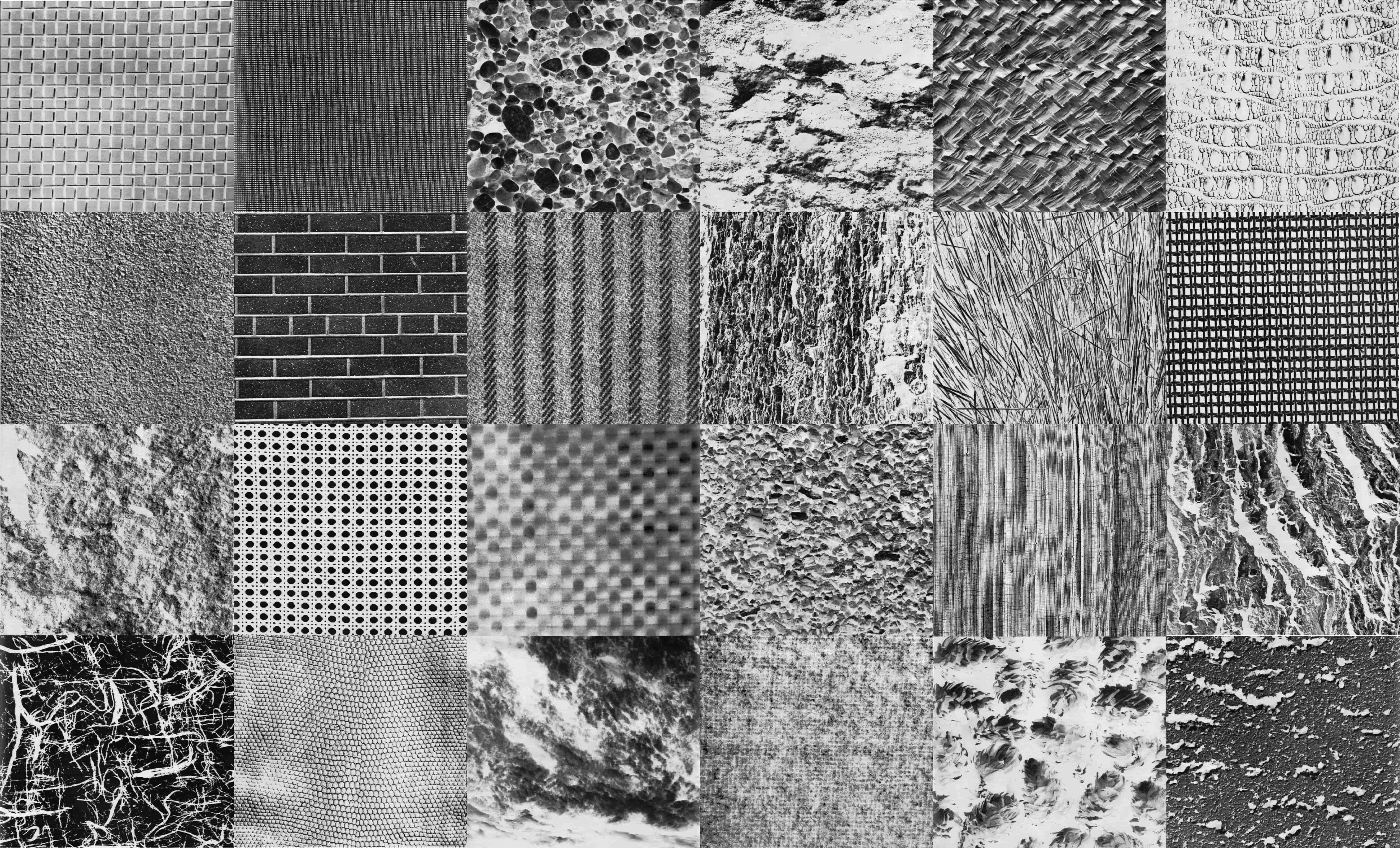
Figure 3: Brodatz data samples.

Yale face data: This YaleExtendedB face data set contains $16128$ face images acquired from $28$ human subjects under varying pose and illumination conditions. We randomly fixed a pose and for that pose consider all the illuminations, leading to $252$ face images taken from $28$ human subjects. We used a similar type of experimental setup as described in [12]. From each face image, we construct a SIFT descriptor [31] and take the first $4$ principal vectors of this descriptor. Thus, each image is identified with a point on the Grassmann manifold of appropriate dimension. And then, inspired by the isometric mapping between the Grassmannian and $\mathcal{P}_{n}$ [24], we construct the covariance descriptor from the aforementioned principal vectors. Here, we used $84$ dictionary atoms.

Figure 4: Yale face data samples.

ETH80 object recognition data: This dataset contains $8$ different objects, each having $10$ different instances from $41$ different views resulting in $3280$ images. We first segment the objects from each image using the provided ground truth. We used both texture and edge features to construct the covariance matrix. For the texture feature, we used three texture filters [25]. The filter bank is $[H_{1}H_{1}^{t},H_{2}H_{2}^{t},H_{3}H_{3}^{t}]$, where $H_{1}=[1,2,1]^{t}$, $H_{2}=[-1,0,1]^{t}$, $H_{3}=[-1,2,-1]^{t}$. In addition to the three texture features, we used the image intensity gradient and the magnitude of the smoothed image using Laplacian of the Gaussian filter. We used $40$ dictionary atoms for this data.

Figure 5: Eth80 data samples.

Performance comparisons are depicted in Tables 2-3 respectively. All of these three methods are intrinsic, i.e., the DL and SC are tailored to the underlying manifold, i.e., $\mathcal{P}_{n}$. In order to compute the reconstruction error, we have used the intrinsic affine invariant metric on $\mathcal{P}_{n}$. From the tables, we can see that SDL yields the best sparsity amongst the three manifold-valued methods (excluding LE-SC). Furthermore, on the Yale-face data set, the SDL is computationally most efficient algorithm when compared to Riem-SC and kStein-SC respectively. In terms of reconstruction error, our proposed method outperforms it’s competitors. Note that, for kStein-SC, computing the reconstruction error is not meaningful as they solved the DLSC problem on the Hilbert space after using a kernel mapping.

Data	SDL		Riem-SC [13]		kStein-SC [23]		LE-SC [21]
	acc. (%)	$\varsigma(\%)$	acc. (%)	$\varsigma(\%)$	acc. (%)	$\varsigma(\%)$	acc. (%)	$\varsigma(\%)$
Brodatz	95.02	95.96	66.21	61.54	88.57	95.40	60.25	98.52
Yale	68.68	92.95	59.98	69.10	53.55	97.58	8.35	99.78
Eth80	96.10	88.07	91.46	78.64	45.79	97.97	45.79	97.97

Table 2: Comparison results on three data sets in terms of classification accuracy and amount of sparsity

Data	SDL		Riem-SC [13]		kStein-SC [23]		LE-SC [21]
	recon. err.	Time(s)	recon. err.	Time(s)	recon. err.	Time(s)	recon. err.	Time(s)
Brodatz	0.55	599.33	1.24	539.63	N/A	527.57	3.21	5.46
Yale	0.001	47.25	0.005	293.91	N/A	131.97	0.25	9.16
Eth80	0.005	153.60	0.017	240.96	N/A	213.93	0.16	3.62

Table 3: Comparison results on three data sets in terms of reonstruction error and computation time

We also depict the comparative performance as a function of number of dictionary atoms, for the four algorithms in Fig. 6 (for Brodatz data) and in Fig. 7 (for the Yale face data set). Here, we have shown the comparative performance in terms of classification accuracy, reconstruction error and required CPU time. For both these data sets, we can see the superior performance of SDL over it’s competitors in terms of classification accuracy and sparsity. As the objective of any DL algorithm is to reconstruct the samples, we have also shown the reconstruction error thereby depicting the competitive performance of SDL over the other algorithms.

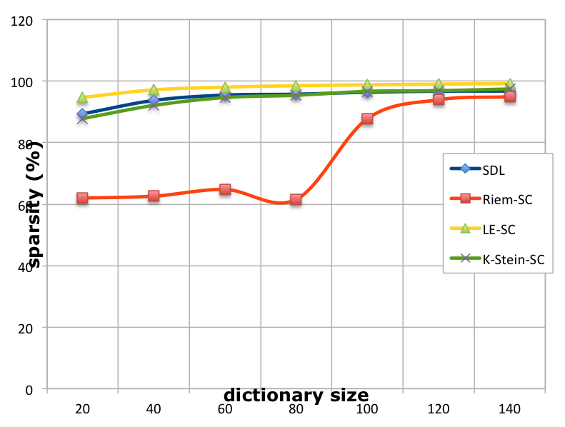
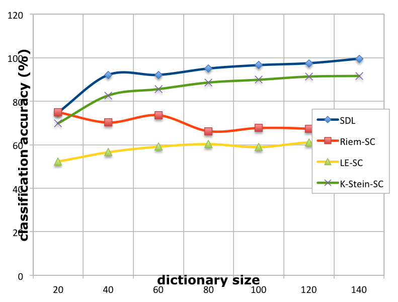
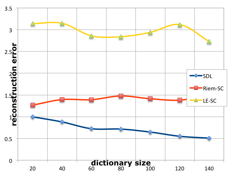
Figure 6: Brodatz data results: Left: Sparsity, Middle: Classification accuracy and Right: Reconstruction error with varying number of dictionary atoms.

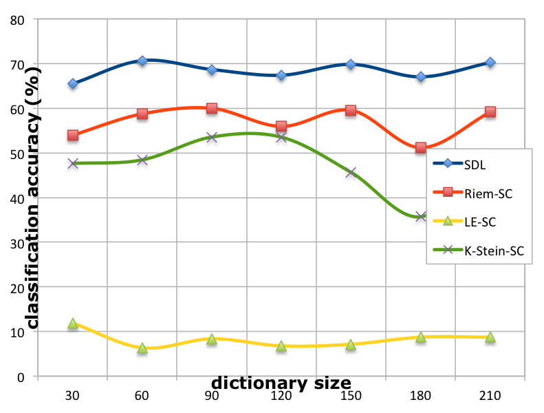
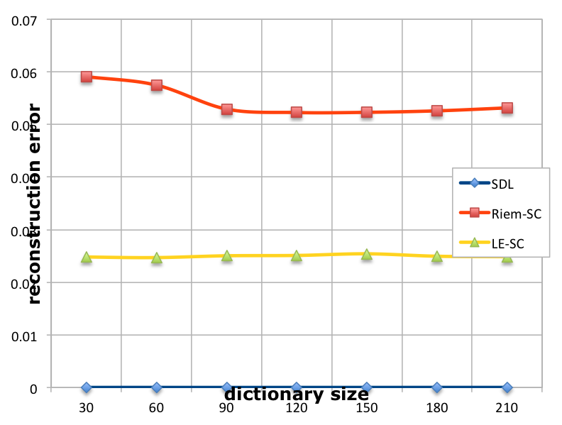
Figure 7: Yale face data results: Left: Sparsity, Middle: Classification accuracy and Right: Reconstruction error with varying number of dictionary atoms.

4 Conclusions

In this paper, we presented an information theoretic dictionary learning and sparse coding algorithm for data residing on a statistical manifold. In the traditional dictionary learning approach on a vector space, the goal is to express each data point as a sparse linear combination of the dictionary atoms. This is typically achieved via the use of a data fidelity term and a term to induce sparsity on the coefficients of the linear combination. In this paper, we proposed an alternative formulation of the DL and SC problem for data residing on statistical manifolds, where we do not have an explicit sparsity constraint in our objective function. Our algorithm, SDL, expresses each data point, which is a probability distribution, as a weighted KL-center of the dictionary atoms. We presented a proof that our proposed formulation yields sparsity without explicit enforcement of this constraint and this result holds true when the KL-divergence is replaced by the Hellinger distance between probability densities. Further, we presented an extension of this formulation to data residing on $\mathcal{P}_{n}$. A Riemannian accelerated gradient descent algorithm was employed to learn the dictionary atoms and an accelerated gradient descent algorithm was employed to learn the sparse weights in a two stage alternating optimization framework. The experimental results demonstrate the effectiveness of the SDL algorithm in terms of reconstruction and classification accuracy as well as sparsity.

Acknowledgements

This research was funded in part by the NSF grants IIS-1525431 and IIS-1724174 to BCV. We thank Dr. Shun-ichi Amari for his insightful comments on a preliminary draft of this manuscript.

References

- [1] Aharon, M., Elad, M., Bruckstein, A.M.: K-svd and its non-negative variant for dictionary design. In: Optics & Photonics 2005. pp. 591411–591411. International Society for Optics and Photonics (2005)
- [2] Akhtar, N., Shafait, F., Mian, A.: Discriminative bayesian dictionary learning for classification. IEEE Transactions on Pattern Analysis and Machine Intelligence 38(12), 2374–2388 (2016)
- [3] Amari, S.i.: Differential-geometrical methods in statistics, vol. 28. Springer Science & Business Media (2012)
- [4] Amari, S.I., Barndorff-Nielsen, O.E., Kass, R., Lauritzen, S., Rao, C.: Differential geometry in statistical inference. Lecture Notes-Monograph Series pp. i–240 (1987)
- [5] Arsigny, V., Fillard, P., Pennec, X., Ayache, N.: Geometric means in a novel vector space structure on symmetric positive-definite matrices. SIMAX 29(1) (2007)
- [6] Basu, A., Harris, I.R., Hjort, N.L., Jones, M.: Robust and efficient estimation by minimising a density power divergence. Biometrika 85(3), 549–559 (1998)
- [7] Brodatz, P.: Textures: a photographic album for artists and designers (1966)
- [8] Bubeck, S.: Theory of convex optimization for ml. arXiv:1405.4980 (2014)
- [9] Candes, E.J., Romberg, J.K., Tao, T.: Stable signal recovery from incomplete and inaccurate measurements. Communications on Pure and Applied Mathematics 59(8), 1207–1223 (2006)
- [10] do Carmo Valero, M.P.: Riemannian geometry (1992)
- [11] Cetingul, H., Vidal, R.: Intrinsic mean shift for clustering on stiefel and grassmann manifolds. In: Proceedings of IEEE Conference on Computer Vision and Pattern Recognition. pp. 1896–1902 (2009)
- [12] Chakraborty, R., Vemuri, B.C.: Recursive fréchet mean computation on grassmannian and its applications to computer vision. ICCV (2015)
- [13] Cherian, A., Sra, S.: Riemannian Sparse Coding for Positive Definite Matrices. European Conference on Computer Vision 8692, 299–314 (2014)
- [14] Cover, T.M., Thomas, J.A.: Elements of information theory (2012)
- [15] Davisson, L., Leon-Garcia, A.: A source matching approach to finding minimax codes. IEEE Transactions on Information Theory 26(2), 166–174 (1980)
- [16] Donoho, D.L., Tsaig, Y., Drori, I., Starck, J.L.: Sparse solution of underdetermined systems of linear equations by stagewise orthogonal matching pursuit. IEEE Transactions on Information Theory 58(2), 1094–1121 (2012)
- [17] ETH80data: https://www.mpi-inf.mpg.de/departments/computer-vision-and-multimodal-computing/research/
- [18] Feragen, A., Lauze, F., Hauberg, S.: Geodesic exponential kernels: When curvature and linearity conflict. In: CVPR. pp. 3032–3042 (2015)
- [19] Fletcher, P.T., Joshi, S.: Riemannian geometry for the statistical analysis of diffusion tensor data. Signal Processing 87(2), 250–262 (2007)
- [20] Gallager, R.G.: Information theory and reliable communication, vol. 2. Springer (1968)
- [21] Guo, K., Ishwar, P., Konrad, J.: Action recognition using sparse representation on covariance manifolds of optical flow. In: AVSS. pp. 188–195 (2010)
- [22] Harandi, M.: Riemannian Coding and Dictionary Learning : Kernels to the Rescue. CVPR pp. 3926–3935 (2015)
- [23] Harandi, M.T., Sanderson, C., Hartley, R., Lovell, B.C.: Sparse Coding and Dictionary Learning for Symmetric Positive Definite Matrices: A Kernel Approach. ECCV 7573, 216–229 (2012)
- [24] Huang, Z., Wang, R., Shan, S., Chen, X.: Projection metric learning on grassmann manifold with application to video based face recognition. In: CVPR. pp. 140–149 (2015)
- [25] Laws, K.I.: Rapid texture identification. In: Annual technical symposium (1980)
- [26] LeCun, Y., Bottou, L., Bengio, Y., Haffner, P.: Gradient-based learning applied to document recognition. Proceedings of the IEEE 86(11), 2278–2324 (1998)
- [27] Lee, K., Ho, J., Kriegman, D.: Acquiring linear subspaces for face recognition under variable lighting. IEEE Transactions on Pattern Analysis and Machine Intelligence 27(5), 684–698 (2005)
- [28] Lenglet, C., Rousson, M., Deriche, R., Faugeras, O.D.: Statistics on the manifold of multivariate normal distributions: Theory and application to diffusion tensor MRI processing. Journal of Mathematical Imaging and Vision 25(3), 423–444 (2006)
- [29] Li, P., Wang, Q., Zuo, W., Zhang, L.: Log-Euclidean Kernels for Sparse Representation and Dictionary Learning. ICCV pp. 1601–1608 (2013)
- [30] Liese, F., Vajda, I.: On divergences and informations in statistics and information theory. IEEE Transactions on Information Theory 52(10), 4394–4412 (2006)
- [31] Lowe, D.G.: Object recognition from local scale-invariant features. In: CVPR. vol. 2, pp. 1150–1157 (1999)
- [32] M., C.: Sinkhorn distances: Lightspeed computation of optimal transport. pp. 2292 – 2300 (2013)
- [33] Mairal, J., Bach, F., Ponce, J., Sapiro, G., Zisserman, A.: Supervised dictionary learning. NIPS pp. 1033–1040 (2009)
- [34] Mairal, J., Bach, F., Ponce, J., Sapiro, G.: Online dictionary learning for sparse coding. In: International Conference on Machine Learning (ICML). pp. 689–696 (2009)
- [35] Mardia, K.V., Jupp, P.E.: Directional Statistics. John Wiley and Sons LTD (2000)
- [36] Moakher, M.: A differential geometric approach to the geometric mean of symmetric positive-definite matrices. SIAM Journal of Matrix Analysis Applications 26(3), 735–747 (2005)
- [37] Qiu, Q., Patel, V.M., Chellappa, R.: Information-theoretic dictionary learning for image classification. IEEE Transactions on Pattern Analysis and Machine Intelligence 36(11), 2173–2184 (2014)
- [38] Rao, C.R.: Fisher-rao metric. Scholarpedia 4(2), 7085 (2009)
- [39] Ryabko, B.Y.: Fast and efficient coding of information sources. IEEE Transactions on Information Theory 40(1), 96–99 (1994)
- [40] Salehian, H., Chakraborty, R., Ofori, E., Vaillancourt, D., Vemuri, B.C.: An efficient recursive estimator of the fréchet mean on a hypersphere with applications to medical image analysis. MICCAI sponsored workshop MFCA (2015)
- [41] Schmitz, M.A., Heitz, M., Bonneel, N., Mboula, F.M.N., Coeurjolly, D., Cuturi, M., Peyré, G., Starck, J.L.: Wasserstein dictionary learning: Optimal transport-based unsupervised non-linear dictionary learning. arXiv preprint arXiv:1708.01955 (2017)
- [42] Schölkopf, B., Smola, A.J.: Learning with kernels: support vector machines, regularization, optimization, and beyond. MIT press (2002)
- [43] Sivalingam, R., Boley, D., Morellas, V., Papanikolopoulos, N.: Tensor sparse coding for region covariances. In: ECCV, pp. 722–735 (2010)
- [44] Spellman, E.: Fusing probability distributions with information theoretic centers and its application to data retrieval. Ph.D. thesis, University of Florida (2005)
- [45] Sra, S., Cherian, A.: Generalized dictionary learning for symmetric positive definite matrices with application to nn retrieval. In: ECML-PKDD (2011)
- [46] Srivastava, A., Jermyn, I., Joshi, S.: Riemannian analysis of probability density functions with applications in vision. In: CVPR. pp. 1–8 (2007)
- [47] Sun, J., Qu, Q., Wright, J.: Complete dictionary recovery over the sphere i: Overview and the geometric picture. IEEE Transactions on Information Theory 63(2), 853–884 (2017)
- [48] Suzuki, M.: Information geometry and statistical manifold. arXiv preprint arXiv:1410.3369 (2014)
- [49] Wang, Z., Vemuri, B.C.: Dti segmentation using an information theoretic tensor dissimilarity measure. IEEE Transaction on Medical Imaging 24(10), 1267–1277 (2005)
- [50] Wright, J., Yang, a.Y., Ganesh, A., Sastry, S.S., Ma, Y.: Robust face recognition via sparse representation. IEEE TPAMI 31(2), 210–227 (2009)
- [51] Wright, J., Ma, Y., Mairal, J., Sapiro, G., Huang, T.S., Yan, S.: Sparse representation for computer vision and pattern recognition. Proceedings of IEEE, Special Issue on Applications of Compressive Sensing & Sparse Representation 98(6), 1031–1044 (2010)
- [52] Xie, Y., Ho, J., Vemuri, B.: On A Nonlinear Generalization of Sparse Coding and Dictionary Learning. ICML 28, 1480–1488 (2013)
- [53] Zhang, F., Cen, Y., Zhao, R., Wang, H., Cen, Y., Cui, L., Hu, S.: Analytic separable dictionary learning based on oblique manifold. Neurocomputing 236, 32–38 (2017)