Dynamics of a polymer under multi-gradient fields

Abstract

Effects of multi-gradient fields on the transport of a polymer chain have been investigated by using generalized Langevin dynamics simulations. We observe that the natural frequency of tumbling follows $Wi^{0.66}$ scaling, where $Wi$ is the Weissenberg number. Analysis of angular tumbling time distribution reveals that the tail of distribution follows exponential distribution and at high Weissenberg number, deviates from Poisson behaviour. Competition between velocity gradient which results shear flow in the system, and solvent quality gradient arising due to the interaction among monomers revealed that there is another scaling associated with the angular tumbling time distribution. Moreover, at low temperature, we observe unusual behaviour that at intermediate shear rates, decay rate $\nu$ decreases with $Wi$.

Multi-factor gradients are essential components of many biological phenomena. They are responsible in coordinating with one another to bring about cell-, time- and location- specific responses in living systems albert . It is realized to be an important, evolutionarily conserved signalling mechanism for guiding the growth, migration, and differentiation of cells within the tissue Thomas . They serve essential roles in inflammation, wound healing, cancer metastasis etc. Insight into the behavior of such systems is of fundamental importance in a wide spectrum of systems ranging from biological cells, where transport appears in varying environments, to shear flow of biomolecules (including bacteria). The presence of shear flow arising due to velocity gradient affects the transport and dispersion of biomolecules at the macroscale Bird ; Doi . Theoretically, de Gennes long back showed that the behavior of coil-stretch transition in polymer is highly dependent on the type of flow degenes . Later Smith and coworkers smith monitored the motion of individual molecules (DNA) under the shear flow. They observed tumbling motion of a polymer chain under shear flow i.e., a DNA undergoes a cyclic stretching and collapse dynamics, with a characteristic frequency which depends on the shear rate and its internal relaxation time. As a result, the dynamics of flexible polymers in shear flow drew considerable interest in recent years schroeder ; Buscalioni ; Doyle ; Winkler ; victor ; sanjib .

A single polymer chain in solution undergoes a transition from the coil (high temperature) state to the globule/folded (low temperature) state degenes1 as the temperature is lowered. It is also possible to study the coil-globule transition by changing the solvent quality i.e. by varying the interaction among monomers. A solvent is called a good solvent if polymer is found to be in the coil state, whereas it is referred as a poor solvent if polymer is in the globule state degenes1 . In addition to velocity gradient, one may think of a system having gradient arising due to the varying environment (solvent quality). In fact, chemotaxis is one of the process arising due to the change in solvent quality (chemical or concentration gradient), which leads to directional motion of cells, bacteria, biomolecules towards or away from a source pnas . Notably, in experimental set-ups as well as in theories, one manipulates shear rate keeping the quality of solvent constant, thereby transport of biomolecules under shear flow is mainly explored by the velocity gradient smith ; schroeder ; Buscalioni ; Doyle ; Winkler ; victor ; sanjib . The aim of this letter is to study the effect of net gradient field arising due to the competition between velocity and chemical potential on the dynamics of polymers, which still remains an unexplored territory. Since, the inclusion of gradient interactions to vary solvent quality in the model system under shear flow hampers the analytical treatment, therefore, we resort to computer simulations to shed light on the rich dynamical behaviour of such systems.

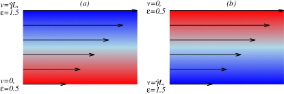
Figure 1: Schematic diagram of flow profile; (a) with a positive gradient of interaction energy $\varepsilon$, both flow velocity, $v$ and interaction energy, $\varepsilon$ increase in the same direction, (b) with a negative gradient of $\varepsilon$ .

We have considered the composite system consisting of polymer of $N(=50)$ beads (appendix A) and fluid (implicit solvent) confined between two walls such that one is stationary and other is moving with velocity $V_{x}$ resulting a velocity gradient in the flow, in the direction perpendicular to wall. The flow velocity experienced by each monomer is $\dot{\gamma}y_{i}$, where $\dot{\gamma}=\frac{dV_{x}}{dy}$, is the velocity gradient (shear rate) along the $y-$ direction. In order to exclude the effect of confinement, we have taken the width of channel greater than 4 time of radius of gyration of polymer. To confine the system in a channel of width $L(=20)$, we have taken the particle-wall interaction (at $y=0$ and $y=L$) in the form of soft repulsion of the Weeks-Chandler-Andersen potential deb . Simulation is carried out in the the reduced units (appendix A). Solvent quality gradient has been incorporated in the model system by linearly varying the interaction energy ($y\Delta\varepsilon$) associated with non-bonded monomers along the $y-$ direction. Fig.1 shows the schematic of flow profile with positive and negative gradient of $\varepsilon$, where value of $\varepsilon$ increases (Fig.1(a)) and decreases (Fig.1(b)) in direction of positive gradient of flow velocity, respectively. Here, we have taken $\Delta\varepsilon=0.05$ in the simulation. A change in color from red to blue (or vice versa) represent a gradient arising due to the change in solvent quality (or temperature). The dynamics of the $i^{th}$ bead of polymer chain (LABEL:sec:Supplementary) in shear flow is described by the generalized Langevin equation (GLE), which explicitly takes into account the effect of coupling to a thermostat to maintain the constant temperature (mcphie ; dobson1 ; dobson2 and appendix A).

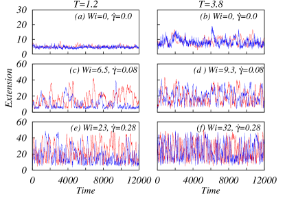
Figure 2: Time history of extension of polymer chain in flow direction at different Wiessenberg number, $Wi$. (a), (c) and (e) at temperature T=1.2 (poor solvent); (b), (d) and (f) at T=3.8 (good solvent) for both cases $\varepsilon$=$Const$ (red color) and $\varepsilon$=$y\Delta\varepsilon$ (blue color).

In absence of flow, a decrease in temperature leads to the coil-globule transition. The ${\theta}-$temperature, $T_{\theta}$ at which this transition takes place, is estimated from the measurement of $\frac{<R_{G}^{2}>}{N}$ at different temperature, where $R_{G}$ is the radius of gyration. The $\theta$ temperature ($\varepsilon=1.0$) has been estimated to be $T_{\theta}=2.5\pm 0.1$. At this temperature $\frac{<R_{G}^{2}>}{N}$ is found to be independent of $N$ murat . We have performed simulation in both regimes i.e. $T>T_{\theta}$ (good solvent) and $T<T_{\theta}$ (poor solvent). The dimensionless flow strength is characterized by the Weissenberg number, $Wi=\dot{\gamma}\tau_{0}$. Here, $\tau_{0}$ is the longest relaxation time of the polymer, which has been determined by fitting the time decay of the autocorrelation function of the end-to-end distance of polymer chain in the absence of a solvent flow. In Fig.2, we have compared the time series of extension of a single chain at different $Wi$ for the uniform solvent quality ($\varepsilon=constant$) and the varying solvent quality ($\varepsilon$=$y\Delta\varepsilon$). Fig.2(a) and (b) show the equilibrium extension ($\dot{\gamma}=0$) of polymer chain in poor ($T=1.2<T_{\theta}$) and good ($T=3.8>T_{\theta}$) solvents, respectively. It is evident from the Fig.2(c) that at low shear rate, polymer chain for varying interaction remains in globule state for a longer time compared to that of the constant interaction ($T<T_{\theta}$). However, at high temperature ($T>T_{\theta}$) there is rapid fluctuations in the extension (Fig.2(d)) for both types of solvent. The maximum extension of polymer depends on the shear rate irrespective of solvent quality. At high shear rate, (Fig.2(e) and (f)) show significant increase in the tumbling events.

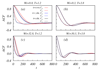
Figure 3: Normalised autocorrelation function (ACF) of the components of end to end vector $\vec{R}$ in flow and gradient direction $C_{x}$, $C_{y}$ for both cases $\varepsilon$=$cons$ and $\varepsilon$=$y\Delta\varepsilon$. (a) and (c) at different $Wi$ at temperature $T$=$1.2$, for poor solvent condition; (b) and (d) at $T$=$3.8$ for good solvent condition.

To study the tumbling dynamics, we calculated the autocorrelation function (ACF) $C_{x}$, $C_{y}$ Schroeder1 ; Buscalioni ; Florencio of components $x$ and $y$ of end to end vector, $\vec{R_{e}}$ in flow and gradient direction respectively, which are defined as $C_{\alpha}(t)=\langle{\delta{R_{\alpha}(t)}\delta{R_{\alpha}(0)}}\rangle/\langle{\delta{R_{\alpha}(0)}\delta{R_{\alpha}(0)}}\rangle$, where $\alpha=x,y$, $\delta{R_{\alpha}(t)}=R_{\alpha}(t)-\langle{R_{\alpha}}\rangle$ and $\langle{.}\rangle$ denotes the time average. Fig.3 shows the ACFs $C_{x}$, $C_{y}$ for both cases $\varepsilon$=$constant$ and $\varepsilon$=$y\Delta\varepsilon$ at temperatures $T=1.2$ and $T=3.8$. One remarkable feature which can be noticed from these plots is that the tumbling dynamics of polymer chain remains insensitive to the positive and negative interaction gradients. Furthermore, the effect of interaction gradient is visible only in the case of poor solvent at low $Wi$. At higher $Wi$, this effect is vanishing and both the ACFs behave similar to the case of $\varepsilon=constant$ (Fig.3(c)). In a good solvent ($T>T_{\theta}$), there is no effect of interaction gradient on ACFs even at lower value of $Wi$ (Fig.3(b) and (d)).

The dynamics of the chain under shear flow is characterised by well defined tumbling events. It is dissipative in nature and arising due to the external forcing similar to the one seen in randomly excited damped oscillator. This analogy may be used to calculate the characteristic time involved in tumbling. The generic form of a damped harmonic oscillator $F(t)=A^{2}cos(w_{d}t+\psi)exp(-\Gamma t)$ was used to fit the ACFs, $C_{x}$ and $C_{y}$ Florencio . The damping rate $\Gamma$, the natural frequency $w_{0}$ ($w_{o}^{2}$=$w_{d}^{2}+\Gamma^{2}$) and the phase constant $\psi$ are the three time parameters. The phase lag $\Delta\psi$=$\psi_{y}-\psi_{x}$ is always positive and gives a new characteristic time $\tau_{lag}=\Delta\psi/w_{d}$, which indicates how fast the chain extension $X$ in shear direction responses to a drag force arising due to the fluctuation in the extension $Y$ in the gradient direction. It is evident from Fig.3(a) that there is an increase in $\tau_{lag}$ at low $Wi$ due to the interaction gradient at low temperature. Values of $w_{d}$, $\Gamma$ and $w_{0}$ obtained from the fits of ACFs ($C_{x}$ and $C_{y}$) for $T=1.2$ (poor solvent) are shown in Fig.4 good . There are significant differences in the values of parameters of both ACFs. Furthermore, the dynamic of chain in flow direction is underdampped ($w_{0}\simeq w_{d}$). However, for low value of $Wi(<30)$, one observes $w_{0}\simeq\Gamma$ in gradient direction. This difference becomes more prominent in presence of interaction gradient i.e. $w_{0}\simeq\Gamma$ and $w_{d}\simeq 0$, while dynamics in flow direction remains unaffected. In all cases, the motion of the chain becomes underdamped as $Wi$ increases ($w_{0}\simeq w_{d}$ and $\Gamma<<w_{0}$). The natural frequency $w_{0}$ is related to tumbling time for tumbling process, succession of coil-stretch cycle, $\tau_{tumb}=\pi/w_{0}$ Florencio . In all cases, irrespective of directions, good or poor solvent quality, absence or presence of interaction gradient, the natural frequency is found to be scaled as $Wi^{2/3}$ for high $Wi$, a robust feature of tumbling dynamics found in previous theoretical and experimental studies schroeder ; victor ; Florencio .

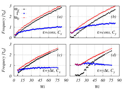
Figure 4: Values of $w_{d}$, $\Gamma$ and $w_{0}$ obtained from fits to ACF ($c_{x}$ and $c_{y}$) for T=1.2 (poor solvent).

Tumbling of chain in shear flow is a stochastic process smith ; Teixeria ; Schroeder1 . The tumbling time, i.e. time interval between subsequent flips of the polymer, is a random variable with relatively large fluctuations. Now onwards, we focus our study on the distribution of angular tumbling time $P(\tau)$, where $\tau$ is the time interval between two subsequent zero crossing of end-to-end distance, $R_{x}=x_{n}-x_{1}$ in the flow direction. For sufficiently large time intervals, it follows exponential distribution, $P(\tau)\approx exp(-\nu\tau)$ (Fig.5), where $\nu$ is the decay rate, its inverse gives the information of $\tau_{tumb}$. This is in agreement with previous studies victor ; celani ; puliafito ; sanjib ; Florencio . Fig.5, shows the distribution of angular tumbling time for different shear rates at low temperature. One can notice a change in slope at shear rate $\approx 0.02$ ($\varepsilon$ = constant) and $0.06$ ($\varepsilon=y\Delta\varepsilon$) in Fig.5(a) and (b), respectively. We identified these values as the critical shear rate, where polymer undergoes a shear induced coil-stretch transition katz . The most interesting feature of the Fig.5(b) is the presence of two time scales at intermediate shear rates for $\varepsilon=y\Delta\varepsilon$, which is absent for $\varepsilon$ = constant.

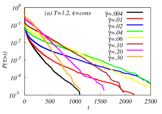
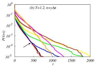
Figure 5: Cumulative distribution of characteristic tumbling time $\tau$ , at different $Wi$ for both cases (a) $\varepsilon$=$cons$ and (b) $\varepsilon$=$y\Delta\varepsilon$, at temperature $T$=$1.2$, for poor solvent condition. Arrow demarcates the emergence of new scaling, which is absent in (a).

Fig.6(a) and (b) show limiting decay rate $\nu$ of tumbling time distribution scaled with relaxation time $\tau_{0}$ with $Wi$ in poor and good solvent respectively. $\tau_{tumb}$ is nearly independent of $Wi$ at low values of $Wi$ and proportional to $\tau_{0}$. At higher $Wi$, $\nu\tau_{0}\approx Wi^{0.75\pm 0.05}$ and $\nu\tau_{0}\approx Wi^{0.85\pm 0.05}$ at high and low temperature, respectively. These exponents are steeper, show non-poissonian behaviour of tumbling process, in agreement with value in Florencio . Surprisingly, at intermediate shear rates (below the critical shear rate), the decay rate decreases with $Wi$. Moreover for $\varepsilon=y\Delta\varepsilon$, the decrease in decay rate is more steeper.

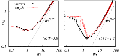
Figure 6: The limiting decay rate, $\nu$ of tumbling time distribution scaled with relaxation time $\tau_{0}$.

In this letter, we have studied for the first time effects of multi-factor gradients on the tumbling dynamics of polymer chain in the free draining limit. We have incorporated the gradient of non-bonded interaction energy parameter, $\varepsilon$ associated with LJ-potential as well as shear flow (velocity gradient) in the model system. In presence of the shear flow, two interesting cases namely positive and negative gradient of $\varepsilon$ with respect to velocity gradient were studied. Surprisingly, there are no notable differences in the tumbling dynamics of chain for both cases. Another interesting observation is that the tumbling dynamics remains invariant for both cases $\varepsilon$ = constant and $\varepsilon=y\Delta\varepsilon$ for poor and good solvent in high shear regime. This is because the energy scale associated with tumbling due to rotation at higher shear rate is much higher than the energy needed to stabilize the polymer conformation. At lower shear rate in poor solvent, where both energy scales are comparable, one observes significant difference in ACFs ($C_{x}$, $C_{y}$), whereas in the good solvent such difference is found to be absent. It is found that the tumbling frequency scales as $Wi^{2/3}$ (Fig.4) consistent with previous studies. Similar scaling is reported if one considers hydrodynamics interaction Florencio ; schroeder . Here, we show that it is the robust feature of the tumbling process irrespective of solvent quality, directions and gradient of chemical potential.

The long tail behavior of tumbling time distribution is found to be exponential with non-poissionian exponent (Fig.6). The exponent for poor solvent is found to be steeper than that of the good solvent. At low shear rates, tumbling time, $\tau_{tumb}$ is nearly independent of shear rate, At very low shear rates, the polymer conformation will be in the collapsed state and its shape is nearly like a sphere of radius $R_{G}$. In this regime, sphere will roll and the work done due to shear force is negligible compare to the interaction energy of polymer beads. As a result, $\tau_{tumb}$ is independent of shear rates. Above the critical shear rate, the work done by shear force is dominant and governs the tumbling dynamics of polymer. Increase in the rotational component of shear flow causes frequent tumbling of polymer accounting the decrease in $\tau_{tumb}$ with increase in shear rate. The most striking feature of present study is the change in the trend of limiting decay rate below the critical shear rate at low temperature. There is decrease in $\nu$ with increase in shear rates. At intermediate shear rate below the critical value, the work done due to shear force now is comparable to the interaction energy, and thus polymer deforms from the sphere like shape to an ellipsoid pointing along the flow direction, which inhibit tumbling. At this point, our work calls for further investigation by including hydrodynamics interaction and effects of chain size on the tumbling dynamics katz .

It may be difficult to implement varying solvent quality in terms of the interaction gradient in vitro similar to the one seen in vivo. However, if one maintains the two surfaces of the channel at two different temperatures, it is possible to achieve the steady state in temperature, which may be thought similar to the interaction gradient. Another way to realize such a gradient in vitro could be due to the differences in the affinity of the salt with the top and bottom surfaces of the channel, which will give rise a salt gradient. One may consider the case of an ionic salt, where electric field gives rise to such gradient. Rheological studies involving isotropic molecules (spherical in shape) and anisotropic molecules (e.g. liquid crystals) may confirm our findings maren1 ; Cates ; Foglino . Therefore, the present studies open several new issues, which warrant further experimental investigations to explore such hitherto unknown scaling related to the tumbling dynamics of polymer under multi-gradient fields, which may have potential applications in understanding the dynamics of active particles.

We thank Garima Mishra and Apratim Chaterjee for many helpful discussions on the subject. We are grateful to P.J. Daivis and Matthew Dobson for their discussions on generalized Langevin equation for this study. The financial assistance from SERB and INSPIRE program of DST, New Delhi, India are gratefully acknowledged.

Appendix A Supplementary material

In the present study, polymer chain is modelled by conventional bead-spring model kremer consisting of N beads where the all non-bonded beads interaction causing excluded volume effect is given by 12-6 Lennard-Jones potential:

$$V_{lj}\left({r}\right)=4\varepsilon\left(\left(\frac{\sigma}{r}\right)^{12}-\ \left(\frac{\sigma}{r}\right)^{6}\right),$$ (1)

where, $r$ is the distance between two monomers, $\varepsilon$ and $\sigma$ characterize the strength of the interaction (potential) and the diameter of monomers, respectively. Throughout the simulation, we have worked in the reduced units, where $\varepsilon=1.0$, $\sigma=1.0$ and $mass=1.0$ are the units of energy, distance and mass of beads, respectively. Units of other quantities are derived in terms of these parameters. Time is measured in units of ${\sigma\left({\frac{m}{\varepsilon}}\right)^{\frac{1}{2}}}$.

All bonded beads experience the finite extensible non linear (FENE) potential and repulsive part of the 12-6 Lennard-Jones(LJ) potential, are given as

$$V_{fene}=-\frac{kR_{0}^{2}}{2}\ln\left(1-\left(\frac{r}{R_{0}}\right)^{2}\right),$$ (2)

$$V_{lj}^{b}\left({r}\right)=4\varepsilon_{b}\left(\left(\frac{\sigma_{b}}{r}\right)^{12}-\ \left(\frac{\sigma_{b}}{r}\right)^{6}\right).$$ (3)

where, $k$ is spring constant and $R_{0}$ is the maximum extension of bond. We set $\varepsilon_{b}=1.0\varepsilon$, $\sigma_{b}=1.0\sigma$ and the values of other parameters are chosen from Ref. kremer in which $R_{0}={1.5\sigma}$, $k=30\frac{\varepsilon}{\sigma^{2}}$.

The cut-off distance of LJ-potential has been implemented by using the following definition of shifted force potential $V_{lj}^{sf}\left({r}\right)$ allen to remove the discontinuity in the potential as well as in the force:

$$V^{sf}\left({r}\right)=\begin{cases}V\left({r}\right)-V\left({r_{c}}\right)-\ \left({\frac{dV\left({r}\right)}{dr}}\right)_{r_{c}}\left({r-r_{c}}\right),r\leq r_{c}\\ 0,~{}~{}~{}~{}~{}~{}~{}~{}~{}~{}~{}~{}~{}~{}~{}~{}~{}~{}~{}~{}~{}~{}~{}~{}~{}~{}~{}~{}~{}~{}~{}~{}~{}~{}~{}~{}~{}~{}~{}~{}~{}~{}r>r_{c}\end{cases}$$ (4)

where $r_{c}$ is the cut-off distance for intermolecular interaction. We set $r_{c}=2.5\sigma$ and $2^{\frac{1}{6}}\sigma_{b}$ in Eqs.(1) and (3), respectively.

The particle-wall interaction (at $y=0$ and $y=L$) of composite system (polymer and fluid) confined between two walls of width $L$ is taken in the form of soft repulsion of the Weeks-Chandler-Andersen potential deb . For the wall at $y=0$,

$$V_{w}=4\varepsilon_{w}\left(\left(\frac{\sigma_{w}}{y}\right)^{12}-\ \left(\frac{\sigma_{w}}{y}\right)^{6}+\frac{1}{4}\right),\ 0\leq y\leq 2^{\frac{1}{6}}\sigma_{w}.$$ (5)

For the wall at $y=L$,

$$V_{w} =4\varepsilon_{w}\left(\left(\frac{\sigma_{w}}{L-y}\right)^{12}-\ \left(\frac{\sigma_{w}}{L-y}\right)^{6}+\frac{1}{4}\right),~{}~{}\text{for}$$

$$~{}~{}~{}~{}~{}~{}~{}~{}~{}~{}~{}~{}~{}~{}~{}~{}~{}~{}~{}~{}~{}~{}~{}~{}~{}~{}~{}~{}~{}~{}~{}~{}L-\sigma_{w}\leq y\leq 2^{\frac{1}{6}}\sigma_{w}$$ (6)

Here, $y$ is the y-coordinate of the bead along the flow gradient. In present simulations, we choose $\sigma_{w}=\frac{\sigma}{2}$ and the parameter $\varepsilon_{w}$ controls the strength of soft repulsion.

The dynamics of the $i^{th}$ bead of polymer chain in shear flow is described by the following Langevin equation:

$$\vec{\ddot{r}}_{i}(t)=\vec{F}_{i}^{c}(t)-\Gamma\left[\vec{\dot{r}}_{i}(t)\ -\dot{\gamma}y_{i}\hat{i}\right]+\dot{\gamma}\dot{y_{i}}\hat{i}+\vec{R}_{i}(t)$$ (7)

This is the generalized Langevin equation (GLE) for a particles in a steady shear flow, which explicitly takes into account the effect of coupling to a thermostat to maintain the steady state mcphie ; dobson1 ; dobson2 . In this equation, the Langevin thermostat is applied to the relative velocity coordinate and then transformed back to the laboratory frame. The first term is the conservative force, $\vec{\triangledown}V$, $V=V_{FENE}+V_{LJ}$. The second and third term represent drag force relative to the flow velocity and force in the x-direction due to the particle’s movement across the streamlines, respectively. The last term is the random force acting on $i^{th}$ bead due to solvent motion is kubo ; mcphie ; dobson1 ; dobson2 :

$$\langle{{\vec{R}_{i}(t)\vec{R}_{j}(t^{\prime})}}\rangle={6K_{B}T\Gamma\delta_{ij}\delta(t-t^{\prime})}.$$ (8)

Eq.(A7) is solved by using a fifth-order predictor corrector method allen , with a time step $\Delta t=0.006$. The simulation has been carried out over a broad range of friction coefficient 0.5 to 8.0. In order to vary $Wi$, one has to change either friction coefficient or shear rate. For a given shear rate, we vary friction coefficient to achieve desire range of $Wi$. We have checked the stability of simulation for long run. We have calculated the temperature from thermal momentum numerically and found that the temperature of the system remains same as of the bath temperature throughout the simulations.

References

- (1) B. Alberts, D. Bray, J. Lewis, M. Raff, K. Roberts and J. D. Watson, Molecular Biology of the Cell, (Garland Publishing: New York, 2002).
- (2) T. M. Keenan and A Folch Lab Chip 8 34 (2008).
- (3) R. B. Bird, R. C. Armstrong, and O. Hassager, Dynamics of Polymeric Liquids, vol. 1: Fluid Mechanics, 2nd ed. (Wiley-Interscience, New York, 1987).
- (4) M. Doi and S. F. Edwards The Theory of Polymer Dynamics, (Oxford University Press, New York, 1986).
- (5) P.G. de Gennes, J. Chem. Phys, 60 5030 (1974).
- (6) D. Smith, H. Babcock and S. Chu, Science, 283 1724 (1999); D. E. Smith and S. Chu, Science 281, 1335 (1998); T. T. Perkins, D. E. Smith and S. Chu, Science, 276, 2016 (1997).
- (7) C. M. Schroeder , R. E. Teixeira, E. S. G. Shaqfe and S. Chu, Phys. Rev. Lett. 95, 018301 (2005).
- (8) R. Delgado-Buscalioni, Phys. Rev. Lett. 96 088303 (2006).
- (9) P. S. Doyle, B. Ladoux, and J-L Viovy, Phys. Rev. Lett. 84, 4769 (2000).
- (10) R. G. Winkler, Phys. Rev. Lett. 97, 128301, (2006).
- (11) S. Gerashchenko and V. Steinberg, Phys. Rev. Lett. 96, 038304 (2006).
- (12) D. Das and S. Sabhapandit, Phys. Rev. Lett. 101, 188301 (2008).
- (13) P. G. de Gennes Scaling concepts in polymer physics(Cornell University Press, Ithaca, 1979).
- (14) R. M. Macnab and D. E. Koshland, PNAS, bf 69 2509 (1972).
- (15) D. Deb, A. Winkler, M. H. Yamani, M. Oettel, P. Virnau, and K. Binder, J.Chem. Phys. 134, 214706 (2011) and references therein.
- (16) M.G. McPhie, P.J. Daivis, I. K. Snook, J. Ennis and D.J. Evans, Physica A 299 412 (2001).
- (17) M. Dobson, F. Legoll, T. Lelivre, and G. Stoltz. ESAIM: M2AN, 47, 1583, (2013)
- (18) Matthew Dobson and Abdel Kader Geraldo, arXiv:1709.08118
- (19) G. S. Grest and M. Murat, Macromolecules, 26, 3108 (1993).
- (20) C.M. Schroeder, R.E. Teixeira, E.S.G. Shaqfeh and S. Chu, Macromolecules 38 1967 (2005).
- (21) F. B. Usabiaga and R. Delgado-Buscalioni, Macromol. Theory Simul., 20, 466 (2011).
- (22) In case of good solvent, the values of and for both ACFs are found to be equal within the error bar.
- (23) R.E. Teixeira, H.P. Babcock, E. Shaqfeh and S. Chu, Macromolecules 38 581 (2005).
- (24) A. Puliafito and K. Turitsyn, Physica D, 211 9 (2005).
- (25) A. Celani, A. Puliafito and K. Turitsyn, Europhys. Lett. 70, 464 (2005)
- (26) A. A. Katz et al Phys. Rev. Lett. 97, 138101 (2006).
- (27) D. Marenduzzo, E. Orlandini, and J. M. Yeomans, Phys. Rev. Lett. 98, 118102 (2007).
- (28) M. E. Cates et al Phys. Rev. Lett. 101, 068102 (2008).
- (29) M. Foglino, A. N. Morozov, Henrich, and D. Marenduzzo Phys. Rev. Lett. 119, 208002 (2017).
- (30) K. Kremer and G.S. Grest, Phys. Rev. A 33, 3628 (1986).
- (31) M. P. Allen and D. J. Tildesley, Computer Simulation of liquids, (1987).
- (32) R. Kubo, Rep. Prog. Phys, 29, 255 (1966).