The Logistic Network Lasso

Abstract

We apply the network Lasso to solve binary classification and clustering problems for network-structured data. To this end, we generalize ordinary logistic regression to non-Euclidean data with an intrinsic network structure. The resulting “logistic network Lasso” amounts to solving a non-smooth convex regularized empirical risk minimization. The risk is measured using the logistic loss incurred over a small set of labeled nodes. For the regularization we propose to use the total variation of the classifier requiring it to conform to the underlying network structure. A scalable implementation the learning method is obtained using an inexact variant of the alternating direction methods of multipliers which results in a scalable learning algorithm.

I Introduction

The recently introduced extension of the least absolute shrinkage and selection operator (Lasso) to network-structured data, coined the “network Lasso” (nLasso), allows efficient processing of massive datasets using modern convex optimization methods [4]. In this paper, we apply nLasso to semi-supervised classification and clustering of massive network-structured datasets (big data over networks) [1, 2, 3].

Most of the existing work on nLasso-based methods focused on predicting numeric labels (or target variables) within regression problems [5, 6, 4, 7, 8, 9]. In contrast, we apply nLasso to binary classification (and clustering) problems which assign binary-valued labels to data points. The resulting logistic nLasso (lnLasso) aims at balancing the empirical error, measured using the logistic loss, incurred for a small number of data points whose labels are known with the amount by which the resulting classifier conforms to the underlying network structure.

Thus, lnLasso is an instance of regularized empirical risk minimization with the total variation of the classifier as regularization term [10]. This minimization problem is a non-smooth convex optimization problem which we solve using an inexact form of the alternating direction method of multipliers (ADMM) [11].

The lnLasso provides an alternative to the family of label propagation (LP) methods [12]. While LP methods are based on using the squared error loss to measure the empirical risk incurred over labeled data points, the lnLasso uses the average logistic loss over the labeled data points to assess the quality of a particular classifier.

While lnLasso is based on a probabilistic model for the labels, it considers the network structure as given and fixed. This is different from the semi-supervised classification method presented in [13]. In particular, [13] applies belief propagation for a stochastic block model (SBM) to semi-supervised classification. This mehtod is an approximation to the Bayes optimal classifier given the probabilistic SBM.

Finally, our method is closely related to graph-cut methods [14, 15, 16]. Indeed, both are based on a similar optimization problem. In contrast to graph-cut methods, our approach provides a precise probabilistic i interpretation of this optimization problem. Moreover, while our implementation of lnLasso is based on convex optimization (allowing for highly scalable implementations), graph-cuts is based on combinatorial optimization.

II Problem Formulation

We consider network-structured datasets that can be represented by an undirected weighted graph (the “empirical graph”) $\mathcal{G}=(\mathcal{V},\mathcal{E},\mathbf{W})$. A particular node $i\in\mathcal{V}$ of the graph represents an individual data point (such as a document, an image or an entire social network user profile). Two different data points $i,j\in\mathcal{V}$ are connected by undirected edges $\{i,j\}\in\mathcal{E}$ if these data points are considered similar (such as the documents authored by the same person or the social network profiles of befriended users).

Each undirected edge $\{i,j\}\in\mathcal{E}$ is associated with a positive weight $W_{ij}>0$ quantifying the amount of similarity between data points $i,j\in\mathcal{V}$. The neighbourhood of a node $i\in\mathcal{V}$ is defined as $\mathcal{N}(i):=\{j:\{i,j\}\in\mathcal{E}\}$. Without essential loss of generality, we only consider datasets with a connected empirical graph $\mathcal{G}$ with more than one node.

It will be useful to think of an undirected edge $\{i,j\}\!\in\!\mathcal{E}$ as a pair of two directed edges $(i,j)$ and $(j,i)$. With a slight abuse of notation we denote by $\mathcal{E}$ the set of undirected edges as well as the set of directed edges obtained by replacing each undirected edge by a pair of directed edges.

On top of the network structure, datasets often convey additional information such as labels $y_{i}$ (e.g., the class membership) of the data points $i\in\mathcal{V}$. In what follows, we focus on binary classification problems involving binary labels $y_{i}\in\{-1,1\}$. Since the acquisition of reliable label information is costly, we typically have access only to few labels $y_{i}$ of the nodes in a small sampling set $\mathcal{M}\!\subset\!\mathcal{V}$.

We model the labels $y_{i}$ of the data points $i\in\mathcal{V}$ as independent random variables with (unknown) probabilities

$$p_{i}:={\rm Prob}\{y_{i}\!=\!1\},$$ (1)

We parametrize these probabilities using the logarithm of the “odds ratio”,

$$x[i]:={\rm log}(p_{i}/(1-p_{i})).$$ (2)

The quantity (2) defines a graph signal $x[\cdot]:\mathcal{V}\rightarrow\mathbb{R}$ assigning each node $i\in\mathcal{V}$ of the empirical graph $\mathcal{G}$ the signal value $x[i]$. Our approach uses a graph signal $x[\cdot]$ to represent a classifier for the data points in $\mathcal{G}$. In particular, we classify a data point $i\in\mathcal{V}$ as $\hat{y}_{i}={\rm sign}\{x[i]\}$. Any reasonable classifier $x[\cdot]$ should agree well with available label information such that $\hat{y}_{i}\approx y_{i}$ for all $i\in\mathcal{M}$.

III Logistic Network Lasso

It is sensible to learn a classifier $x[\cdot]:\mathcal{V}\rightarrow\mathbb{R}$ from few initial labels $\{y_{i}\}_{i\in\mathcal{M}}$ by maximizing their probability (evidence), or equivalently by minimizing the empirical error

$$\widehat{E}(x[\cdot])\!:=\!\frac{1}{\left|\mathcal{M}\right|}\sum_{i\in\mathcal{M}}\!\ell(y_{i}x[i])$$ (3)

with the logistic loss function

$$\ell(z):={\rm log}(1+\exp(-z)).\vspace*{-1mm}$$ (4)

The criterion (3) by itself is not sufficient for guiding the learning of a classifier $x[\cdot]$ based on the labels $\{y_{i}\}_{i\in\mathcal{M}}$. Indeed, the criterion (3) ignores the signal values $x[i]$ at non-sampled nodes $i\in\mathcal{V}\setminus\mathcal{M}$.

In order to learn an entire classifier $x[\cdot]$ from the incomplete information provided by the initial labels $\{y_{i}\}_{i\in\mathcal{M}}$, we need to impose some additional structure on the classifier $x[\cdot]$. In particular, any reasonable classifier $x[\cdot]$ should conform with the cluster structure of the empirical graph $\mathcal{G}$ [17].

The extend to which a graph signal $x[\cdot]$ conforms with the cluster structure is measured by the total variation (TV)

$$\|x[\cdot]\|_{\rm TV} :=\sum_{\{i,j\}\in\mathcal{E}}W_{ij}\left|x[j]-x[i]\right|.$$ (5)

Indeed, a graph signal $x[\cdot]$ has a small TV only if the signal values $x[i]$ are approximately constant over well connected subsets (clusters) of nodes.

We are led quite naturally to learning a classifier $x[\cdot]$ via the following regularized empirical risk minimization

$$\hat{x}[\cdot] \in\operatorname*{argmin}_{x[\cdot]\in\mathbb{R}^{\mathcal{V}}}\widehat{E}(x[\cdot])+\lambda\|x[\cdot]\|_{\rm TV}.$$ (6)

The regularization parameter $\lambda$ in (6) allows to trade-off a small TV $\|\hat{x}[\cdot]\|_{\rm TV}$ of the classifier $\hat{x}[\cdot]$ against a small empirical error $\widehat{E}(\hat{x}[\cdot])$ (cf. (3)). We refer to (6) as the logistic nLasso (lnLasso) problem. The choice of $\lambda$ can be guided by cross validation techniques [18].

Note that lnLasso (6) does not enforce directly the labels $y_{i}$ to be clustered. Instead, it requires the classifier $x[\cdot]$ (which parametrizes the probability distributed of the labels $y_{i}$ via (2)) to be clustered (have a small TV).

IV Implementation via Inexact ADMM

We now present a classification method which is obtained by solving (6) using inexact ADMM. To this end, we introduce for each directed edge $(i,j)\in\mathcal{E}$ of the oriented empirical graph $\mathcal{G}$, the auxiliary variable $z_{ij}$. These variables act as local copies of the optimization variables $x[i]$ in (6).

We can then reformulate lnLasso (6) as (cf. (5))

$$\hat{x}[\cdot]\in \operatorname*{argmin}_{x[\cdot]\in\mathbb{R}^{\mathcal{V}}}\widehat{E}(x[\cdot])+(\lambda/2)\sum_{(i,j)\in\mathcal{E}}W_{i,j}|z_{ij}-z_{ji}|$$ (7)

$$\text{s.t.}\indent x[i]=z_{ij}\indent i\in\mathcal{V},\indent j\in\mathcal{N}(i).$$ (8)

The reformulation (7) of the lnLasso (6) is computationally appealing since the objective function in (7) consists of two independent terms. The first term is the empirical risk $\widehat{E}(x[\cdot])$ which measures how well the initial labels $y_{i}$ agree with the classifier $x[\cdot]$. The second term is the scaled TV $\lambda\sum_{(i,j)\in\mathcal{E}}W_{i,j}|z_{ij}-z_{ji}|$, which measures how well the classifier $x[\cdot]$ is aligned with the cluster structure of $\mathcal{G}$. These two terms are coupled via (8).

In order to solve the non-smooth convex optimization problem (7), we apply an inexact variant of ADMM [19]. To this end, we define the augmented Lagrangian [11]

$$\mathcal{L}(x[\cdot],z_{ij},u_{ij}) :=\widehat{E}(x[\cdot])+(\lambda/2)\sum_{(i,j)\in\mathcal{E}}W_{ij}\left|z_{ij}-z_{ji}\right|$$ (9)

$$+\!(\rho/2)\sum_{(i,j)\in\mathcal{E}}\big{[}(x[i]\!-\!z_{ij}\!+\!u_{ij})^{2}\!-\!u_{ij}^{2}\big{]}$$

with dual variables $u_{ij}$ introduced for each edge $(i,j)\in\mathcal{E}$.

Ordinary (exact) ADMM optimizes $\mathcal{L}(x[\cdot],z_{ij},u_{ij})$ block coordinate-wise by iterating the following updates:

$$x^{(k+1)}[\cdot] \!:=\!\operatorname*{argmin}_{x[\cdot]\in\mathbb{R}^{\mathcal{V}}}\mathcal{L}(x[\cdot],z_{ij}^{(k)},u_{ij}^{(k)})$$ (10)

$$z^{(k+1)}_{ij} \!:=\!\operatorname*{argmin}_{z_{ij}\in\mathbb{R}}\mathcal{L}(x^{(k+1)}[\cdot],z_{ij},u_{ij}^{(k)})$$ (11)

$$u^{(k+1)}_{ij} \!:=\!u^{(k)}_{ij}\!+\!x^{(k+1)}[i]\!-\!z^{(k+1)}_{ij}\mbox{ for each }(i,j)\!\in\!\mathcal{E}.$$ (12)

The update (10) minimizes the empirical error $\widehat{E}(x[\cdot])$, while update (11) minimizes the TV $\|x[\cdot]\|_{\rm TV}$. These two minimization processes are coupled via (12) using the dual variables $\{u_{ij}\}_{(i,j)\in\mathcal{E}}$. Each dual variable $u_{i,j}$ corresponds to a particular directed edge $(i,j)\in\mathcal{E}$ and the corresponding constraint $x[i]=z_{ij}$ (see (8)).

Using the masked labels $\tilde{y}_{i}\!=\!y_{i}\!\in\!\{-1,1\}$ for sampled nodes $i\in\mathcal{M}$ and $\tilde{y}_{i}=0$ otherwise, the update (10) becomes

$$x^{(k\!+\!1)}[i]\!=\!\operatorname*{argmin}_{x\in\mathbb{R}}\underbrace{\ell(\tilde{y}_{i}x)\!+\!\frac{|\mathcal{M}|\rho}{2}\sum_{j\in\mathcal{N}(i)}(x\!-\!z_{ij}^{(k)}\!+\!u_{ij}^{(k)})^{2}}_{:=f_{i}(x)}.$$ (13)

The update (11) can be worked out as (see, e.g., [4])

$${z}_{ij}^{(k+1)}\!=\!\theta({x}^{(k\!+\!1)}[i]\!+\!{u}_{ij}^{(k)})\!+\!(1\!-\!\theta)({x}^{(k+1)}[j]\!+\!{u}_{ji}^{(k)})$$

with

$$\theta\!=\!\max\left(\frac{1}{2},1-\frac{(\lambda/\rho)W_{ij}}{|{x}^{(k+1)}[i]\!+\!{u}_{ij}^{(k)}\!-\!{x}^{(k+1)}[j]\!-\!{u}_{ji}^{(k)}|}\right).$$

The presence of the logistic loss function (4) precludes a closed-form solution of (13). However, since (13) amounts to a scalar unconstrained smooth minimization, we can solve (13) approximately by cheap iterative methods. Replacing the ADMM update (13) by an inexact update might still yield convergence to the solution of (7) [20, Theorem 8].

As we will show, (13) can be approximated by

$$\hat{x}^{(k\!+\!1)}[i]\!=\underbrace{\Phi_{i}\circ\ldots\circ\Phi_{i}}_{|\tilde{y}_{i}|\lceil 2\log(2(k\!+\!1))/\log(|\mathcal{M}|\rho d_{i})\rceil}(1/d_{i})\sum_{j\in\mathcal{N}(i)}\big{(}z^{(k)}_{ij}\!-\!u^{(k)}_{ij}\big{)}$$ (14)

with the node degree $d_{i}=|\mathcal{N}(i)|$ and the map

$$\Phi_{i}(x)\!:=\!\frac{\tilde{y}_{i}/(|\mathcal{M}|d_{i}\rho)}{1\!+\!\exp(\tilde{y}_{i}x)}\!+\!(1/d_{i})\sum_{j\in\mathcal{N}(i)}\big{(}z^{(k)}_{ij}\!-\!u^{(k)}_{ij}\big{)}.$$ (15)

Replacing the update (13) with (14) yields Alg. 1.

Algorithm 1 lnLasso via inexact ADMM

1:$\mathcal{G}$, $\mathcal{M}$, $\{y_{i}\}_{i\in\mathcal{M}}$, $\lambda$, $\rho$

2:Initialize:$k\!:=\!0$, $x^{(0)}[i]\!:=\!0$, $z^{(0)}_{ij}\!:=\!0$, $u^{(0)}_{ij}\!:=\!0$, $\tilde{y}_{i}\!:=\!0$, $\tilde{y}_{i}:=y_{i}$ for all sampled nodes $i\in\mathcal{M}$

3:repeat

4:     for $i\in\mathcal{V}$ do

5:         set $\tilde{x}^{(0)}\!:=\!(1/d_{i})\sum\limits_{j\in\mathcal{N}(i)}(z_{ij}^{(k)}\!-\!u_{ij}^{(k)})$

6:         set $n:=0$

7:         repeat

8:              $\tilde{x}^{(n+1)}:=\Phi_{i}(\tilde{x}^{(n)})$ (see (15))

9:              $n:=n+1$

10:         until $n\geq\lceil|\tilde{y}_{i}|2\log(2(k\!+\!1))/\log(|\mathcal{M}|\rho d_{i})\rceil$

11:         $\hat{x}^{(k+1)}[i]:=\tilde{x}^{(n)}$

12:     end for

13:     for  $(i,j)\in\mathcal{E}$ do

14:         $\theta:=\max\bigg{\{}1/2,1\!-\!\frac{(\lambda/\rho)W_{ij}}{|\hat{x}^{(k\!+\!1)}[i]\!+\!{u}^{(k)}_{ij}\!-\!\hat{x}^{(k\!+\!1)}[j]\!-\!{u}^{(k)}_{ji}|}\bigg{\}}$

15:          ${z}_{ij}^{(k\!+\!1)}\!:=\!\theta(\hat{x}^{(k\!+\!1)}[i]\!+\!{u}_{ij}^{(k)})\!+\!(1\!-\!\theta)(\hat{x}^{(k\!+\!1)}[j]\!+\!{u}_{ji}^{(k)})$

16:          ${u}_{ij}^{(k\!+\!1)}:={u}_{ij}^{(k)}\!+\!(\hat{x}^{(k\!+\!1)}[i]\!-\!{z}_{ij}^{(k\!+\!1)})$

17:     end for

18:     $k\!:=\!k\!+\!1$

19:until convergence

20:classifier $\hat{x}[i]:=\hat{x}^{(k)}[i]$ for all $i\in\mathcal{V}$

The classifier $\hat{x}[i]$ delivered by Alg. 1 is then used to label the data points as $\hat{y}_{i}=1$ if $\hat{x}[i]>0$ and $\hat{y}_{i}=-1$ otherwise. However, the classifier $\hat{x}[i]$ provides more information than just the resulting (predicted) labels $\hat{y}_{i}$.

Indeed, the magnitudes $|\hat{x}[i]|$ quantify the confidence in the predicted labels $y_{i}$. A magnitude $|\hat{x}[i]|$ close to zero indicates the predicted label $\hat{y}_{i}$ to be unreliable. On the other hand, if the magnitude $|\hat{x}[i]|$ is large then we can be quite confident in the predicted label $\hat{y}_{i}$.

The convergence of the iterates $\hat{x}^{(k)}[i]$ generated by Alg. 1 to the solution $\hat{x}[i]$ of the lnLasso problem (7) can be verified from [20, Theorem 8]. In particular, convergence is guaranteed (for any $\rho>0$) if the errors $\varepsilon_{k}=|\hat{x}^{(k+1)}[i]-x^{(k+1)}[i]|$ are sufficiently small such that $\sum_{k=1}^{\infty}\varepsilon_{k}<\infty$. The following result verifies exactly this condition.

Lemma 1.

For $|\mathcal{M}|\rho d_{i}>1$, the deviation between the inexact and exact updates (14) and (13) satisfies

$$|\hat{x}^{(k\!+\!1)}[i]\!-\!x^{(k\!+\!1)}[i]|\leq 1/(k\!+\!1)^{2}.$$ (16)

Proof.

The update (13) is an unconstrained minimization of a differentiable convex function $f_{i}(x)$. The solutions $x_{0}$ of (13) are solutions of $f^{\prime}_{i}(x_{0})=0$ [21]. Working out the derivative $f^{\prime}_{i}(x)$, this “zero-gradient condition” becomes

$$\frac{-\tilde{y}_{i}}{1\!+\!\exp(\tilde{y}_{i}x_{0})}\!+\!|\mathcal{M}|\rho\sum_{j\in\mathcal{N}(i)}(x_{0}\!-\!z_{ij}^{(k)}\!+\!u_{ij}^{(k)})=0.$$ (17)

The necessary and sufficient condition (17) for $x_{0}$ to solve (13) is, in turn, equivalent to the fixed-point characterization

$$x_{0}=\Phi_{i}(x_{0}),\vspace*{-2mm}$$ (18)

with the map $\Phi_{i}$ defined in (15).

The approximate update (14) is a fixed-point iteration [22, 23] for solving (18). The map $\Phi_{i}$ (15) is a contraction over the interval $[b_{i}\!-\!1,b_{i}\!+\!1]$ with the shorthand $b_{i}:=(1/d_{i})\sum_{j\in\mathcal{N}(i)}(z_{ij}^{(k)}\!-\!u_{ij}^{(k)})$. In particular,

$$\Phi_{i}([b_{i}\!-\!1,b_{i}\!+\!1])\subseteq[b_{i}\!-\!1,b_{i}\!+\!1]\vspace*{-2mm}$$

and

$$|\Phi_{i}(x)\!-\!\Phi_{i}(x^{\prime})|\!\leq\!|x\!-\!x^{\prime}|/(|\mathcal{M}|\rho d_{i})\mbox{ for }x,x^{\prime}\!\in\![b_{i}\!-\!1,b_{i}\!+\!1].\vspace*{0mm}$$

The bound (16) follows then from standard results on fixed-point iterations (see, e.g., [22, Thm. 1.48]). ∎

Note that Alg. 1 is highly scalable as it can be implemented using message passing over the empirical graph $\mathcal{G}_{\rm syn}$.

V Numerical Experiments

We assess the performance of lnLasso (Alg. 1) by means of numerical experiments using a synthetic dataset whose network structure conforms to the stochastic block model (SBM). In particular, we consider a dataset (of size $N=500$) whose empirical graph $\mathcal{G}$ is generated according to a SBM with two clusters $\mathcal{C}_{1}$, $\mathcal{C}_{2}$. The nodes are assigned to these two clusters (blocks) randomly with equal probability $1/2$. Two nodes within the same group are connected with probability $c_{\rm in}/N$ while nodes of different groups are connected with probability $c_{\rm out}/N$.

The weights of edges connecting nodes within cluster $\mathcal{C}_{1}$ are chosen as $W_{i,j}\sim[\mathcal{N}(10,1)]_{+}$ and the weights for edges within cluster $\mathcal{C}_{2}$ as $W_{i,j}\sim[\mathcal{N}(12,1)]_{+}$. The weights of boundary edges $\{i,j\}\in\partial\mathcal{F}$ are drawn according to $W_{i,j}\sim[\mathcal{N}(3,1)]_{+}$. The true underlying labels $y_{i}=1$ for $i\in\mathcal{C}_{1}$ and $y_{i}=-1$ for $i\in\mathcal{C}_{2}$ are observed only for nodes in the sampling set $\mathcal{M}$ selected uniformly at random.

The experiments involve $K\!=\!1000$ i.i.d. realizations of the empirical graph $\mathcal{G}$ and sampling set $\mathcal{M}$. For each realization of $\mathcal{G}$ and $\mathcal{M}$, we execute lnLasso with $\lambda=2\cdot 10^{-5}$ and $\rho=1$ (which implies the condition $|\mathcal{M}|d_{i}\rho>1$ required by Lemma 1). For comparison, we also implemented belief propagation (BP) for SBM [13], plain vanilla LP [24] and the max-flow (graph-cut) method [16].

In Fig. 1, we plot the average classification accuracies (rate of correct labels) achieved by the various methods for varying ratio $\epsilon\!=\!c_{\rm in}/c_{\rm out}$ of the SBM used to generate the empirical graph. Choosing $\epsilon\approx 1$ corresponds to a weak cluster structure, while for $\epsilon\!\gg\!1$ the cluster structure is strongly pronounced. The shaded areas in Fig. 1 indicate the empirical standard deviation obtained over the $1000$ simulation runs.

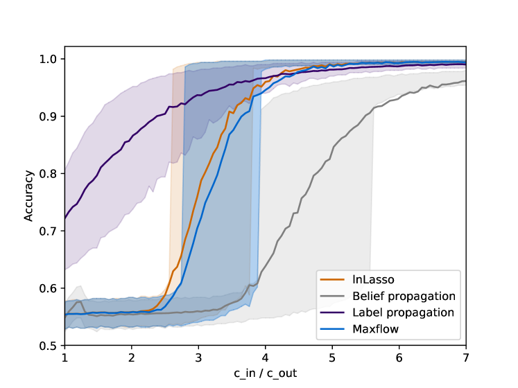
Figure 1: Classification accuracy for varying $c_{\rm in}/c_{\rm out}$.

According to Fig. 1, lnLasso performs poor relative to LP for $\epsilon\!<\!2.5$, while for $\epsilon\!>\!4$, lnLasso (along with the max-flow method) slightly outperforms LP. Moreover, our results suggest that lnLasso is more robust regarding the variations in the precise network structure compared to BP.

In Fig. 2, for the SBM with $\epsilon\!=\!5$, we depict the classification accuracy as a function of the amount of labeled nodes (selected uniformly at random) quantified by the sampling ratio $\alpha\!=\!|\mathcal{M}|/N$. The solid lines represent the average accuracies obtained for $1000$ simulation runs. For small sampling sets ($\alpha\ll 1$) the classification accuracy of lnLasso is poor compared to LP. However, for $\alpha\!>\!1/20$ lnLasso becomes significantly more accurate and for $\alpha\!>\!1/10$ even slightly outperforms LP. Overall, lnLasso is slightly better than max-flow and significantly better than BP.

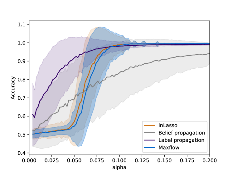
Figure 2: Classification accuracy for varying sampling ratio $\alpha$.

In a second experiment we compared LP with lnLasso on a dataset whose empirical graph is a chain. This chain graph is partitioned into two clusters $\mathcal{C}_{1}=\{1,\ldots,50\}$ and $\mathcal{C}_{2}=\{51,\ldots,100\}$. Edges within the same cluster have weight $W_{i,i+1}=1$, while the boundary edge $\{50,51\}$ has weight $W_{50,51}=1/2$. The nodes are labeled as $y_{i}=-1$ for $i\in\mathcal{C}_{1}$ and $y_{i}=1$ for $i\in\mathcal{C}_{2}$. We observe the labels only for the sampling set $\mathcal{M}=\{10,60\}$.

In Fig. 4, we depict the resulting classifiers obtained from LP and lnLasso (Alg. 1 with $\rho=1$ and $\lambda=1/10$), each running for $1000$ iterations. In contrast to LP, lnLasso recovers the cluster structure perfectly.

In a third experiment we use lnLasso to perform forground extraction on images. We represent a RGB image as a grid graph with each node representing a particular pixel. The nodes are connected to their nearest neighbours. Each node is associated a label $y=1$ if the corresponding pixel is foreground and $y=-1$ if the pixel is background. In Fig. 3, we show the result by highlighting pixel $i$ according to the classifier value $x[i]$.

Figure 3: The foreground extracted by lnLasso.

Figure 4: LP and lnLasso for chain graph.

VI Conclusions

We proposed the lnLasso for classifying network-structured datasets. In contrast to LP, which uses the squared error loss, lnLasso uses the logistic loss to within regularized empirical risk minimization. The regularization term of lnLasso is the TV of the classifier requiring it to conform with the cluster structure of the empirical graph. A scalable implementation of lnLasso is obtained via inexact ADMM. The effectiveness of lnLasso to learn the labels of network-structured data is assessed by means of illustrative numerical experiments. Our work opens several avenues for future research: We plan to extend the current approach for binary classification to multi-class and multi-label problems. Moreover, we aim at analysing the statistical properties of lnLasso. This analysis would help to guide the choice of the regularization parameter in lnLasso.

References

- [1] S. Bhagat, C. Graham, and S. Muthukrishnan, Social network data analytics, Springer, 2011.
- [2] L. Lovász, “Large networks and graph limits,” American Mathematical Society, vol. 60, 2012.
- [3] S. Cui, A. Hero, Z.-Q. Luo, and J.M.F. Moura, Eds., Big Data over Networks, Cambridge Univ. Press, 2016.
- [4] D. Hallac, J. Leskovec, and S. Boyd, “Network lasso: Clustering and optimization in large graphs,” in Proc. SIGKDD, 2015, pp. 387–396.
- [5] A. Jung, N.T. Quang, and A. Mara, “When is network lasso accurate?,” Frontiers in Appl. Math. and Stat., vol. 3, pp. 28, 2018.
- [6] A. Jung and M. Hulsebos, “The network nullspace property for compressed sensing of big data over networks,” Front. Appl. Math. Stat., Apr. 2018.
- [7] S. Chen, A. Sandryhaila, J. M. F. Moura, and J. Kovačević, “Signal recovery on graphs: Variation minimization,” IEEE Trans. Signal Processing, vol. 63, no. 17, pp. 4609–4624, Sept. 2015.
- [8] A. Sandryhaila and J. M. F. Moura, “Big data analysis with signal processing on graphs: Representation and processing of massive data sets with irregular structure,” IEEE Signal Processing Magazine, vol. 31, no. 5, pp. 80–90, Sept 2014.
- [9] A. Jung, “On the complexity of sparse label propagation,” Front. Appl. Math. Stat., Jul. 2018.
- [10] V. N. Vapnik, The Nature of Statistical Learning Theory, Springer, 1999.
- [11] S. Boyd, N. Parikh, E. Chu, B. Peleato, and J. Eckstein, Distributed Optimization and Statistical Learning via the Alternating Direction Method of Multipliers, vol. 3 of Foundations and Trends in Machine Learning, Now Publishers, Hanover, MA, 2010.
- [12] O. Chapelle, B. Schölkopf, and A. Zien, Eds., Semi-Supervised Learning, The MIT Press, Cambridge, Massachusetts, 2006.
- [13] P. Zhang, C. Moore, and L. Zdeborova, “Phase transitions in semisupervised clustering of sparse networks,” arXiv, 2014.
- [14] P. Ruusuvuori, T. Manninen, and H. Huttunen, “Image segmentation using sparse logistic regression with spatial prior,” in 2012 Proceedings of the 20th European Signal Processing Conference (EUSIPCO), Aug. 2012, pp. 2253–2257.
- [15] R. K chichian, S. Valette, and M. Desvignes, “Automatic multiorgan segmentation via multiscale registration and graph cut,” IEEE Transactions on Medical Imaging, pp. 1–1, 2018.
- [16] Y. Boykov and V. Kolmogorov, “An experimental comparison of min-cut/max- flow algorithms for energy minimization in vision,” IEEE Transactions on Pattern Analysis and Machine Intelligence, vol. 26, no. 9, pp. 1124–1137, Sept. 2004.
- [17] M. E. J. Newman, Networks: An Introduction, Oxford Univ. Press, 2010.
- [18] T. Hastie, R. Tibshirani, and J. Friedman, The Elements of Statistical Learning, Springer Series in Statistics. Springer, New York, NY, USA, 2001.
- [19] J. Eckstein and W. Yao, “Approximate ADMM algorithms derived from Lagrangian splitting,” Computational Optimization and Applications, vol. 68, no. 2, pp. 363 – 405, Nov. 2017.
- [20] J. Eckstein and D. P. Bertsekas, “On the Douglas-Rachford splitting method and the proximal point algorithm for maximal monotone operators,” Math. Program., vol. 55, no. 3, pp. 293–318, June 1992.
- [21] S. Boyd and L. Vandenberghe, Convex Optimization, Cambridge Univ. Press, Cambridge, UK, 2004.
- [22] H. H. Bauschke and P. L. Combettes, Convex Analysis and Monotone Operator Theory in Hilbert Spaces, Springer, New York, 2011.
- [23] A. Jung, “A fixed-point of view on gradient methods for big data,” Frontiers in Applied Mathematics and Statistics, vol. 3, 2017.
- [24] X. Zhu and Z. Ghahramani, “Learning from labeled and unlabeled data with label propagation,” Tech. Rep., 2002.