Geometry of limits of zeros
of polynomial sequences of type $(1,1)$

Abstract.

In this paper, we study the root distribution of some univariate polynomials satisfying a recurrence of order two with linear polynomial coefficients. We show that the set of non-isolated limits of zeros of the polynomials is either an arc, or a circle, or a “lollipop”, or an interval. As an application, we discover a sufficient and necessary condition for the universal real-rootedness of the polynomials, subject to certain sign condition on the coefficients of the recurrence. Moreover, we obtain the sharp bound for all the zeros when they are real.

1. Introduction

Root distribution of polynomials in a sequence discover intensive information about the interrelations of the polynomials in the sequence, especially when the sequence satisfies a recurrence. Stanley [14] provides some figures for the root distribution of some polynomials in a sequence arising from combinatorics.

In the study of the root distribution of sequential polynomials, both the real-rootedness and the limiting distribution of zeros of the polynomials receive much attention. Some evidence for the significance of real-rootedness of polynomials can be found in Stanley [15, §4]. Bleher and Mallison [6] consider the zeros of Taylor polynomials, and the asymptotics of the zeros for linear combinations of exponentials. Some study on certain “zero attractor” of particular sequences of polynomials can be found in [7, 10]. The exploration of zero attractors of Appell polynomials has been regarded as “gems in experimental mathematics” in [8]. Limiting distribution of zeros has been used to study the four-color theorem via the chromatic polynomials initiated by Birkhoff [5], which amounts to the nonexistence of a chromatic polynomial with a zero at the point $4$. Beraha and Kahane [2] examine the limits of zeros for the sequence of chromatic polynomials of a special family of $3$-regular graphs, described as to consist of an inner and outer square separated by $n$ $4$-rings. It turns out that the number $4$ is a limit of zeros of polynomials in this family.

Motived by the LCGD conjecture from topological graph theory, Gross, Mansour, Tucker and the first author [11, 12] study the root distribution of polynomials satisfying the recurrence

(1.1) $$W_{n}(z)=A(z)W_{n-1}(z)+B(z)W_{n-2}(z),$$

where the functions $A(z)$ and $B(z)$ are polynomials such that one of them is linear and that the other is constant. They established the real-rootedness subject to some sign conditions of the coefficients of $A(z)$ and $B(z)$. Since the real-rootedness implies the log-concavity, they confirm the LCGD conjecture for many graph families whose genus polynomials satisfy Eq. 1.1 with the sign conditions. Orthogonal polynomials and quasi-orthogonal polynomials have closed relations with Eq. 1.1; see Andrews, Richard and Ranjan [1] and Brezinski, Driver and Redivo-Zaglia [9]. Jin and Wang [13] characterized the common zeros of polynomials $W_{n}(z)$ for general $A(z)$ and $B(z)$.

Following Gross et al. [11], a sequence $\{W_{n}(z)\}_{n}$ of polynomials satisfying Eq. 1.1 is said to be of type $(\deg A(z),\,\deg B(z))$. It is normalized if $W_{0}(z)=1$ and $W_{1}(z)=z$. When $A(z)=az+b$ and $B(z)=cz+d$ are linear, Eq. 1.1 reduces to

(1.2) $$W_{n}(z)=(az+b)W_{n-1}(z)+(cz+d)W_{n-2}(z).$$

Concentrating on the root distribution, and considering the polynomials defined by $(-1)^{n}W_{n}(-z)$, one may suppose without loss of generality that $c\geq 0$. We use a quadruple $(\operatorname{\mathrm{sgn}}(a),\operatorname{\mathrm{sgn}}(b),\operatorname{\mathrm{sgn}}(c),\operatorname{\mathrm{sgn}}(d))$, each coordinate of which is either $+$ or $-$ or $0$, to denote the combination of signs of the numbers $a,b,c,d$.

Gross et al. [11, 12], establish the real-rootedness for Cases $(+,*,0,-)$, $(0,+,+,+)$ and $(0,+,+,-)$, where the symbol $*$ indicates that the number $b$ might be of any sign. In Case $(-,-,+,-)$, Wang and Zhang [17] establish the real-rootedness of all polynomials $W_{n}(z)$ for when $\Delta_{g}>0$, where $\Delta_{g}=(b+c)^{2}+4d(1-a)$. In Case $(+,+,+,+)$, they [18] show that every polynomial $W_{n}(z)$ is real-rooted if and only if $ad\leq bc$.

According to Beraha, Kahane, and Weiss’ result [3, 4] on limits of zeros of polynomials satisfying Eq. 1.1, polynomials satisfying Eq. 1.2 have at most two isolated limits of zeros. In this paper, we show that the set of non-isolated limits of zeros of polynomials satisfying Eq. 1.2 is either an arc, or a circle, or a “lollipop”, or an interval. As an application, we can show that in Case $(+,-,+,-)$, every polynomial is real-rooted if and only if $ad\leq bc$. Moreover, when the isolated limits are real, the zeros approach to them in an oscillating manner in Cases $(0,+,+,+)$ and $(+,+,+,+)$, that is, from both the left and right sides of the isolated limits, while the convergence way is from only one side in Case $(+,-,+,-)$; see Theorem 3.4.

We should mention that the generating function of the normalized polynomials satisfying Eq. 1.1 is

$$\sum_{n\geq 0}W_{n}(z)t^{n}=\frac{1+(z-A(z))t}{1-A(z)t-B(z)t^{2}}.$$

In comparison, the root distribution of the polynomials generated by the function

$$\sum_{n\geq 0}W_{n}(z)t^{n}=\frac{1}{1-A(z)t-B(z)t^{2}}$$

has been investigated in [16], in which Tran found an algebraic curve containing the zeros of all polynomials $W_{n}(z)$ with large subscript $n$.

This paper is organised as follows. After reviewing necessary notion and and notation, we interpret Beraha et al.’s characterization for polynomials satisfying Eq. 1.2 in Theorem 2.3. In §3, we provide a sufficient and necessary condition of real-rootedness in Case $(+,-,+,-)$, and the root distribution when they are real-rooted as an application of Theorem 2.3.

2. Geometry of the limits of zeros

Throughout this paper, we let $a,b,c,d\in\mathbb{R}$, $ac\neq 0$, and let $\{W_{n}(z)\}_{n\geq 0}$ be a sequence of polynomials satisfying Eq. 1.2. Then the polynomial $W_{n}(z)$ has leading term $a^{n-1}z^{n}$. For any complex number $z=re^{i\theta}$ with $\theta\in(-\pi,\pi]$, we use the square root notation $\sqrt{z}$ to denote the number $\sqrt{r}e^{i\theta/2}$, which lies in the right half-plane $\theta\in(-\pi/2,\,\pi/2]$. The general formula in 2.1 is the base of our study, which can be found in [11, 12].

Lemma 2.1.

Let $A,B\in\mathbb{C}$. Suppose that $W_{0}=1$ and $W_{n}=AW_{n-1}+BW_{n-2}$ for $n\geq 2$. Then

$$W_{n}=\begin{cases}{\displaystyle{\alpha_{+}\lambda_{+}^{n}+\alpha_{-}\lambda_{-}^{n}}},&\textrm{ if $\Delta\neq 0$},\\[5.0pt] {\displaystyle{A+nh\over 2}\cdot\biggl{(}{{A\over 2}}\biggr{)}^{n-1}},&\textrm{ if $\Delta=0$},\end{cases}$$

for $n\geq 0$, where $h=2W_{1}-A$ and

$$\lambda_{\pm}=\frac{A\pm\sqrt{\Delta}}{2},\qquad\alpha_{\pm}=\frac{\sqrt{\Delta}\pm h}{2\sqrt{\Delta}},\qquad\text{with $\Delta=A^{2}+4B$}.$$

Accordingly, we employ the notations

$$\Delta(z) =A(z)^{2}+4B(z)=a^{2}z^{2}+(2ab+4c)z+(b^{2}+4d),$$

$$h(z) =2W_{1}(z)-A(z)=(2-a)z-b,$$

$$\lambda_{\pm}(z) =\frac{A(z)\pm\sqrt{\Delta(z)}}{2},$$

$$\alpha_{\pm}(z) =\frac{\sqrt{\Delta(z)}\pm h(z)}{2\sqrt{\Delta(z)}},$$

$$g(z) =-\alpha_{+}(z)\alpha_{-}(z)\Delta(z)=\frac{h^{2}(z)-\Delta(z)}{4}=(1-a)z^{2}-(b+c)z-d.$$

Denote by $x_{A}=-b/a$ and $x_{B}=-d/c$ the zeros of $A(z)$ and $B(z)$ respectively. The function $\Delta(z)$ has two zeros

$$x_{\Delta}^{\pm}=x_{A}+\frac{-2c\pm 2\sqrt{\Delta_{\Delta}}}{a^{2}},$$

where $\Delta_{\Delta}=c^{2}-a^{2}B(x_{A})$ is the discriminant of $\Delta(z)$. A number $z^{*}\in\mathbb{C}$ is a limit of zeros of the sequence $\{W_{n}(z)\}_{n}$ of polynomials if there is a zero $z_{n}$ of $W_{n}(z)$ for each $n$ such that $\lim_{n\to\infty}z_{n}=z^{*}$.

Lemma 2.2 (Beraha et al. [3]).

Under the non-degeneracy conditions

1. the sequence $\{W_{n}(z)\}_{n}$ does not satisfy a recurrence of order less than two,

2. $\lambda_{+}(z)\neq\omega\lambda_{-}(z)$ for some $z\in\mathbb{C}$ and some constant $\omega$ such that $|\omega|=1$,

a number $z$ is a limit of zeros if and only if it satisfies one of the following conditions:

1. $\alpha_{-}(z)=0$ and $\lambda_{+}(z)<\lambda_{-}(z)$;

2. $\alpha_{+}(z)=0$ and $\lambda_{+}(z)>\lambda_{-}(z)$;

3. $\lambda_{+}(z)=\lambda_{-}(z)$.

A limit $z$ of zeros is said to be non-isolated if it satisfies Item (C-iii), and to be isolated if it satisfies Item (C-i) or Item (C-ii). We denote the set of non-isolated limits of zeros of the polynomials $W_{n}(z)$ by $\clubsuit$, and denote the set of isolated limits of zeros by $\spadesuit$. The clover symbol $\clubsuit$ is adopted for the leaflets of a clover are not alone, while the spade symbol $\spadesuit$ appearing as a single leaflet represents isolation in comparison.

Theorem 2.3.

Let $a,b,c,d\in\mathbb{R}$ and $ac\neq 0$. Let $\{W_{n}(z)\}_{n}$ be a sequence of polynomials satisfying Eq. 1.2 with $W_{0}(z)=1$ and $W_{1}(z)=z$. Then the sets of isolated and non-isolated limits of zeros of $\{W_{n}(z)\}_{n}$ are respectively

$$\spadesuit =\{z\in\mathbb{C}\colon g(z)=0,\,\Re\bigl{(}{A(z)\overline{h(z)}}\bigr{)}<0\}\quad\hbox{ and }\quad$$

$$\clubsuit =\begin{cases}\wideparen{x_{\Delta}^{-}x_{A}x_{\Delta}^{+}},&\text{if $\Delta_{\Delta}<0$};\\[5.0pt] C_{0},&\text{if $\Delta_{\Delta}=0$};\\[5.0pt] J_{\Delta}\cup C_{0},&\text{if $\Delta_{\Delta}>0$ and $B(x_{A})>0$};\\[5.0pt] J_{\Delta},&\text{if $\Delta_{\Delta}>0$ and $B(x_{A})\leq 0$};\end{cases}$$

where $\overline{z}$ denotes the complex conjugate of $z$, $\wideparen{x_{\Delta}^{-}x_{A}x_{\Delta}^{+}}$ stands for the circular arc connecting the points $x_{\Delta}^{-}$ and $x_{\Delta}^{+}$, through the point $x_{A}$,

$$C_{0}=\{z\in\mathbb{C}\colon\lvert z-x_{B}\rvert=\lvert x_{A}-x_{B}\rvert\}$$

is the circle with center $x_{B}$ and radius $\lvert x_{A}-x_{B}\rvert$, and

$$J_{\Delta}=\{x\in\mathbb{R}\colon x_{\Delta}^{-}\leq x\leq x_{\Delta}^{+}\}$$

is an interval.

Proof.

Item (N-i) is satisfied since otherwise one would have $W_{n}(z)=z^{n}$ for each $n$, contradicting the fact $W_{2}(z)=az^{2}+(b+c)z+d$. Item (N-ii) holds true since $|\lambda_{-}(x)|\neq|\lambda_{+}(x)|$ for sufficiently large real number $x$.

Suppose that $z\in\spadesuit$. From definition, we have $\alpha_{-}(z)\alpha_{+}(z)=0$, which implies

$$0=g(z)=\frac{h^{2}(z)-\Delta(z)}{4}.$$

Thus $\sqrt{\Delta(z)}\in\{\pm h(z)\}$. If $\sqrt{\Delta(z)}=h(z)$, then $\alpha_{-}(z)=0$ from definition. By 2.2, we have $\lambda_{+}(z)<\lambda_{-}(z)$, i.e., $\Re\bigl{(}{A(z)\overline{h(z)}}\bigr{)}<0$. Along the same line we can handle the other case $\sqrt{\Delta(z)}=-h(z)$.

It is clear that $\{x_{A},\,x_{\Delta}^{-},\,x_{\Delta}^{+}\}\subseteq\clubsuit$. Let $z=x+yi\in\clubsuit$ such that $A(z)\Delta(z)\neq 0$, where $x,y\in\mathbb{R}$. If $y=0$, then $z,\,A(z),\,\Delta(z)\in\mathbb{R}$. In this case, we can infer that

$$\lambda_{-}(z)=\lambda_{+}(z)\quad\iff\quad\Delta(z)<0\quad\iff\quad\Delta_{\Delta}>0\;\text{and}\;x\in(x_{\Delta}^{-},\,x_{\Delta}^{+}).$$

Otherwise $y\neq 0$. We can infer that

$$\lambda_{-}(z)=\lambda_{+}(z) \iff\text{the vectors $A(z)$ and $\sqrt{\Delta(z)}$ are orthogonal}$$

$$\iff\text{the vectors $A^{2}(z)$ and $\Delta(z)$ have opposite directions}$$

$$\iff\text{$A^{2}(z)$ and $B(z)$ have opposite directions, $\lvert A^{2}(z)\rvert<\lvert 4B(z)\rvert$}$$

$$\iff\begin{cases}\Re A^{2}(z)\cdot\Im B(z)=\Re B(z)\cdot\Im A^{2}(z)\\[5.0pt] \Im A^{2}(z)\cdot\Im B(z)<0\\[5.0pt] \lvert\Im A^{2}(z)\rvert<4\lvert\Im B(z)\rvert\end{cases}$$

$$\iff\begin{cases}\,(x-x_{B})^{2}+y^{2}=(x_{A}-x_{B})^{2}\\ (x-x_{A})(x-x_{A}+2c/a^{2})<0\end{cases}$$

$$\iff z\in C_{0}\cap S_{0}\setminus\{x_{A},\,x_{\Delta}^{-},\,x_{\Delta}^{+}\},$$

where $S_{0}=\{z\in\mathbb{C}\colon\lvert\Re z-x_{A}\rvert\leq\lvert 2c/a^{2}\rvert,\,c\cdotp(\Re z-x_{A})\leq 0\}$ is the vertical strip with boundaries $\Re z=x_{A}$ and $\Re z=x_{A}-2c/a^{2}$. It is clear that the boundary $\Re z=x_{A}$ intersects the circle $C_{0}$ at the point $x_{A}$. To figure out the intersection of the other boundary with $C_{0}$, we proceed according to the sign of $\Delta_{\Delta}$.

Suppose that $\Delta_{\Delta}<0$. Then $J_{\Delta}=\emptyset$ from definition, and

$$\Re\bigl{(}{x_{\Delta}^{\pm}}\bigr{)}=x_{A}-\frac{2c}{a^{2}}\quad\hbox{ and }\quad\Im\bigl{(}{x_{\Delta}^{\pm}}\bigr{)}=\pm\frac{2\sqrt{-\Delta_{\Delta}}}{a^{2}}.$$

It follows that

$$\bigl{(}{x_{\Delta}^{\pm}-x_{B}}\bigr{)}^{2}=\biggl{(}{x_{A}-\frac{2c}{a^{2}}-x_{B}}\biggr{)}^{2}+\biggl{(}\frac{2\sqrt{-\Delta_{\Delta}}}{a^{2}}\biggr{)}^{2}=(x_{A}-x_{B})^{2}.$$

Thus the points $x_{\Delta}^{\pm}$ lie on the intersection of the boundary $\Re z=x_{A}-2c/a^{2}$ and the circle $C_{0}$. Since the intersection contains at most two points, the points $x_{\Delta}^{\pm}$ consitute the intersection. Hence the set $\clubsuit=C_{0}\cap S_{0}$ is the circular arc $\wideparen{x_{\Delta}^{-}x_{A}x_{\Delta}^{+}}$.

When $\Delta_{\Delta}=0$, the points $x_{\Delta}^{\pm}=x_{A}-2c/a^{2}$ coincide with each other. As a consequence, we have $C_{0}\cap S_{0}=C_{0}$ and $\clubsuit=J_{\Delta}\cup C_{0}=C_{0}$.

Below we can suppose that $\Delta_{\Delta}>0$. Note that

(2.1) $$B(x_{A})=c(x_{A}-x_{B}).$$

When $B(x_{A})\leq 0$, we claim that $C_{0}\cap S_{0}=\{x_{A}\}$. Let $z\in C_{0}\cap S_{0}$. If $c>0$, then $x_{A}\leq x_{B}$ by Eq. 2.1. Since $z\in C_{0}$, we have $\Re z\geq x_{A}$. Since $z\in S_{0}$, we have $c(\Re z-x_{A})\leq 0$. Therefore, we infer that $\Re z=x_{A}$, and $z=x_{A}$ consequently. Otherwise $c<0$. Then $x_{A}\geq x_{B}$ by Eq. 2.1. In this case, $z\in C_{0}$ implies $\Re z\leq x_{A}$, and $z\in S_{0}$ implies $\Re z\geq x_{A}$. Hence $z=x_{A}$ for the same reason. This proves the claim. Since $\Delta(x_{A})=4B(x_{A})\leq 0$, we have $x_{A}\in J_{\Delta}$. Hence $\clubsuit=J_{\Delta}$.

When $B(x_{A})>0$, we claim that $C_{0}\subset S_{0}$. Let $z\in C_{0}$. One may show $c(\Re z-x_{A})\leq 0$ in the same fashion as when $B(x_{A})<0$. By geometric interpretation and the condition $\Delta_{\Delta}>0$, we deduce that

$$|\Re z-x_{A}|\leq(\text{the diameter of $C_{0}$})=2|x_{A}-x_{B}|<|2c/a^{2}|.$$

This proves the claim and hence $\clubsuit=J_{\Delta}\cup C_{0}$. ∎

We remark that $z\in\spadesuit$ if and only if $\overline{z}\in\spadesuit$. Since $\Delta_{\Delta}\leq 0$ implies $B(x_{A})>0$, the case “$\Delta>0$ and $B(x_{A})\leq 0$” in Theorem 2.3 can be reduced to “$B(x_{A})\leq 0$”.

Corollary 2.4.

Let $a,b,c,d\in\mathbb{R}$ and $ac\neq 0$. Let $\{W_{n}(z)\}_{n}$ be a sequence of polynomials satisfying Eq. 1.2 with $W_{0}(z)=1$ and $W_{1}(z)=z$. If every polynomial $W_{n}(z)$ for large $n$ is real-rooted, then $B(x_{A})\leq 0$, and $\Delta\geq 0$ as a consequence.

Proof.

Since every polynomial $W_{n}(z)$ for large $n$ is real-rooted, we have $\spadesuit\cup\clubsuit\subset\mathbb{R}$. By Theorem 2.3, we find either $\clubsuit=J_{\Delta}$, or $\clubsuit=C_{0}$ and $C_{0}$ degenerates to a single point. In the former case, we find $B(x_{A})\leq 0$. In the latter case, we have $\Delta_{\Delta}=0$ and $x_{A}=x_{B}$, which is impossible since otherwise

$$0=\Delta_{\Delta}=c^{2}-a^{2}B(x_{A})=c^{2},$$

a contradiction. This completes the proof. ∎

When $\clubsuit=J_{\Delta}\cup C_{0}$, it turns out that the set $\clubsuit$ looks like a lollipop; see Fig. 2.1.

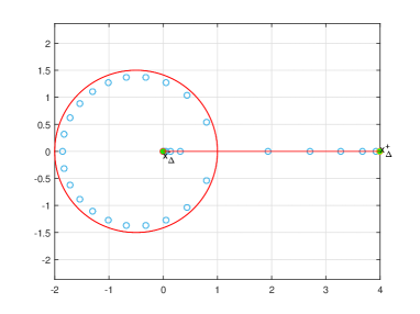
Figure 2.1. The zero distribution of $W_{30}(z)$ for the parameters $(a,b,c,d)=(1,\,-2,\,2,\,-1)$ and $(a,b,c,d)=(1,\,2,\,-2,\,-1)$, for each of which we have $x_{A}=-2$, $x_{B}=-1/2$, and $B(x_{A})=3$.

Theorem 2.5.

Suppose $\Delta_{\Delta}>0$ and $B(x_{A})>0$.† Then $J_{\Delta}\cap C_{0}=\{2x_{B}-x_{A}\}$, and the part of $J_{\Delta}$ outside the circle $C_{0}$ is longer than the part of $J_{\Delta}$ inside $C_{0}$.

Proof.

By Theorem 2.3, we have $\clubsuit=J_{\Delta}\cup C_{0}$. First of all, denote $x_{0}=2x_{B}-x_{A}$ to be one of the two real points on $C_{0}$, other than $x_{A}$. Since

$$\Delta(x_{0})=-\frac{4B(x_{A})\Delta_{\Delta}}{c^{2}}<0,$$

we have $x_{0}\in J_{\Delta}$. Second, the centre of the circle $C_{0}$ is not on the interval $J_{\Delta}$ since $\Delta(x_{B})=A^{2}(x_{B})>0$. It follows that $J_{\Delta}\cap C_{0}=\{x_{0}\}$. Thirdly, note that

(2.2) $$x_{0}-\frac{x_{\Delta}^{-}+x_{\Delta}^{+}}{2}=\frac{1}{c}\cdot\frac{2\Delta_{\Delta}}{a^{2}}.$$

If $c>0$, then $x_{B}<x_{A}$ by Eq. 2.1. It follows that $x_{0}<x_{B}$. Thus the interval $J_{\Delta}$ intersects the circle $C_{0}$ from the left of $C_{0}$. By Eq. 2.2, we have $x_{0}>(x_{\Delta}^{-}+x_{\Delta}^{+})/2$. Thus the part of $J_{\Delta}$ outside the circle $C_{0}$ is longer than the part of $J_{\Delta}$ inside. The other case $c<0$ can be handled in the same way. ∎

3. The interlacing zeros for Case $(+,-,+,-)$

Here is the main result of this section.

Theorem 3.1.

Let $a,c>0$ and $b,d<0$. Let $\{W_{n}(z)\}_{n}$ be a sequence of polynomials satisfying Eq. 1.2 with $W_{0}(z)=1$ and $W_{1}(z)=z$. Then $W_{n}(z)$ is real-rooted if and only if $x_{A}\leq x_{B}$.

The necessity part of Theorem 3.1 can be seen directly from 2.4. The sufficiency part will be handled for the case $x_{A}<x_{B}$ in Theorem 3.4, and for the case $x_{A}=x_{B}$ in Theorem 3.6. Throughout this section, we suppose that $x_{A}\leq x_{B}$, which implies that $\Delta_{\Delta}>0$ and $x_{\Delta}^{\pm}\in\mathbb{R}$. The zeros of the function $g(z)$ are

$$x_{g}^{\pm}=\begin{cases}\displaystyle\frac{b+c}{2(1-a)}\pm\frac{\sqrt{\Delta_{g}}}{2\lvert 1-a\rvert},&\text{if $a\neq 1$},\\[8.0pt] \displaystyle-{d\over b+c},&\text{if $a=1$ and $b+c\neq 0$},\end{cases}$$

where $\Delta_{g}=(b+c)^{2}+4d(1-a)$. We define two numbers $u$ and $v$ by

(3.1) $$(u,v)=\begin{cases}(x_{\Delta}^{-},\,x_{\Delta}^{+}),&\text{if $a<2$ and $F\leq 0$};\\[4.0pt] (x_{g}^{-},\,x_{g}^{+}),&\text{if $a>2$ and $F<0$};\\[4.0pt] (x_{g}^{+},\,x_{\Delta}^{+}),&\text{if $a<1$ and $F>0$};\\[4.0pt] (x_{g}^{-},\,x_{\Delta}^{+}),&\text{otherwise};\end{cases}$$

where $F=\Delta_{g}-\Delta_{\Delta}=d(a-2)^{2}+bc(2-a)+b^{2}$. Note that $(u,v)=(x_{\Delta}^{-},\,x_{\Delta}^{+})$ if $a=1$ and $b+c=0$. Furthermore, we have $u,v\in\mathbb{R}$ since $\Delta_{g}>\Delta_{\Delta}>0$ whenever $a\geq 2$ or $F>0$. As will be seen in Theorems 3.4 and 3.6, we have $u<v$ and the interval $(u,v)$ is the best bound for the zeros of $W_{n}(z)$.

3.1. Case $x_{A}<x_{B}$

We determine the signs of $W_{n}(u)$ and $W_{n}(v)$ in 3.2.

Lemma 3.2.

Let $a,c>0$ and $b,d<0$. Let $\{W_{n}(z)\}_{n}$ be a sequence of polynomials satisfying Eq. 1.2 with $W_{0}(z)=1$ and $W_{1}(z)=z$. Suppose that $x_{A}<x_{B}$. Then we have

(3.2) $$u\leq x_{\Delta}^{-}<x_{A}<x_{\Delta}^{+}\leq v<x_{B},$$

(3.3) $$u<0<v,$$

(3.4) $$W_{n}(u)(-1)^{n}>0,$$

(3.5) $$W_{n}(v)>0,\quad\hbox{ and }\quad$$

(3.6) $$\{u,v\}\subseteq\spadesuit\cup\clubsuit.$$

Proof.

The premise $x_{A}<x_{B}$ implies $\Delta(x_{A})=4B(x_{A})<0$. It follows that

$$x_{A}\in(x_{\Delta}^{-},\,x_{\Delta}^{+}),\qquad x_{\Delta}^{+}>0,\qquad A(x_{\Delta}^{+})>0>A(x_{\Delta}^{-}),\quad\hbox{ and }\quad$$

(3.7) $$h(x_{\Delta}^{+})=(2-a)x_{\Delta}^{+}-b\geq-b>0\qquad\text{if $a\leq 2$}.$$

Since $\Delta(x_{B})=A^{2}(x_{B})>0$ and $x_{\Delta}^{-}<x_{A}<x_{B}$, we have $x_{\Delta}^{+}<x_{B}$.

To confirm Relation (3.6), by Theorem 2.3, it suffices to show that

(3.8) $$A(x)h(x)<0,\qquad\text{for any $x\in\{u,v\}\backslash\{x_{\Delta}^{-},\,x_{\Delta}^{+}\}$}.$$

Let $x_{h}$ be the unique zero of the function $h(z)$ when $a\neq 2$. Then $x_{h}=b/(2-a)$. We proceed according to the definition of the numbers $u$ and $v$.

Case 3.2.1.

$a<2$, $F\leq 0$ and $[u,v]=J_{\Delta}$. It is routine to compute that

(3.9) $$h(x_{\Delta}^{-})h(x_{\Delta}^{+})=\frac{4F}{a^{2}}.$$

Together with Eq. 3.7, we have $h(x_{\Delta}^{-})\leq 0$ and thus

$$x_{\Delta}^{-}\leq x_{h}=\frac{b}{2-a}<0,$$

verifying Eq. 3.3. By 2.1, we have

(3.10) $$W_{n}(x_{\Delta}^{\pm})=\frac{A(x_{\Delta}^{\pm})+nh(x_{\Delta}^{\pm})}{2}\cdot\biggl{(}{\frac{A(x_{\Delta}^{\pm})}{2}}\biggr{)}^{n-1},$$

which implies Eqs. 3.4 and 3.5.

Case 3.2.2.

$a>2$, $F<0$ and $[u,v]=[x_{g}^{-},\,x_{g}^{+}]$. Observe that

(3.11) $$g(x_{\Delta}^{\pm})=\frac{h^{2}(x_{\Delta}^{\pm})}{4}\geq 0.$$

Since the polynomial $g(z)$ is quadratic with leading coefficient negative, we can derive all inequalities in (3.2) except $v<x_{B}$. Since $F<0$, we have $d(a-2)-bc<0$ and thus

$$g(x_{B})=\frac{-d}{c^{2}}\bigl{(}{(a-1)d-bc}\bigr{)}<\frac{-d}{c^{2}}\bigl{(}{(a-2)d-bc}\bigr{)}<0.$$

Since $x_{g}^{-}<x_{A}<x_{B}$, we infer that $x_{g}^{+}<x_{B}$.

On the other hand, by Vièta’s theorem, we have

(3.12) $$x_{g}^{-}x_{g}^{+}=\frac{d}{a-1},$$

whose negativity verifies Eq. 3.3. By 2.1, we have

(3.13) $$W_{n}(x_{g}^{\pm})=(x_{g}^{\pm})^{n},$$

which implies Eqs. 3.4 and 3.5. It is routine to compute that

(3.14) $$h(x_{g}^{-})h(x_{g}^{+})=\frac{F}{a-1}\qquad\text{if $a\neq 1$}.$$

Thus $h(v)<0<h(u)$. By (3.2), we have $A(u)<0<A(v)$. This proves Eq. 3.8.

Case 3.2.3.

$a<1$, $F>0$ and $[u,v]=[x_{g}^{+},\,x_{\Delta}^{+}]$. In view of Eqs. 3.10, 3.13 and 3.7, to confirm Eqs. 3.2, 3.3, 3.4, 3.5 and 3.8, we shall show that

$$x_{g}^{+}\leq x_{\Delta}^{-},\qquad x_{g}^{+}<0,\quad\hbox{ and }\quad h(x_{g}^{+})>0.$$

In fact, we note that the polynomial $g(z)$ is quadratic with leading coefficient positive. On the one hand, Eq. 3.14 gives $x_{h}\in(x_{g}^{-},\,x_{g}^{+})$. This confirms $h(x_{g}^{+})>0$ immediately. By Eq. 3.9, we can deduce that $x_{h}<x_{\Delta}^{-}$, since otherwise one would have the absurd inequality

$$0<x_{\Delta}^{+}<x_{h}=\frac{b}{2-a}<0.$$

Thus Eq. 3.11 implies $(x_{g}^{-},\,x_{g}^{+})\cap J_{\Delta}=\emptyset$. Moreover, the whole interval $(x_{g}^{-},\,x_{g}^{+})$ lies to the left of $J_{\Delta}$. This proves $x_{g}^{+}\leq x_{\Delta}^{-}$. On the other hand, by Eq. 3.12 we have $x_{g}^{-}x_{g}^{+}>0$. Since $x_{g}^{-}<x_{h}<0$, we find $x_{g}^{+}<0$.

Case 3.2.4.

For all remaining cases we have $[u,v]=[x_{g}^{-},\,x_{\Delta}^{+}]$. This time, to confirm Eqs. 3.2, 3.3, 3.4, 3.5 and 3.8, we shall show that

$$x_{g}^{-}\leq x_{\Delta}^{-},\qquad x_{g}^{-}<0,\qquad h(x_{\Delta}^{+})\geq 0,\quad\hbox{ and }\quad h(x_{g}^{-})>0.$$

In fact, when $a=1$, in view of Case 3.2.1, we now have $F>0$ and thus $b+c<0$. Note that $g(z)=-(b+c)z-d$. It follows from Eq. 3.11 that $x_{g}^{-}\leq x_{\Delta}^{-}$. Since $g(0)=-d>0$, we obtain $x_{g}^{-}<0$. By Eq. 3.7, we have $h(x_{\Delta}^{+})\geq 0$. It is routine to compute that

$$h(x_{g}^{-})=x_{g}^{-}-b=-\frac{d}{b+c}-b=-\frac{F}{b+c}>0.$$

Now, in view of Cases 3.2.1 and 3.2.3, we have $a>1$. Consequently, one may derive $J_{\Delta}\subseteq[x_{g}^{-},\,x_{g}^{+}]$ and $x_{g}^{-}<0$ as in Case 3.2.2. We shall handle the two inequalities involving $h$ according to the value range of $a$. If $a=2$, then the function $h(z)=-b$ reduces to a positive constant and we are done. Now we can suppose that $a\neq 2$.

1. If $a>2$, then

   $$h(x_{\Delta}^{-})+h(x_{\Delta}^{+})=\frac{4}{a^{2}}\bigl{(}{(a-2)c-ab}\bigr{)}>0.$$

   In view of Case 3.2.2, we have $F\geq 0$. By Eq. 3.9, we have $h(x_{\Delta}^{-})h(x_{\Delta}^{+})\geq 0$. Therefore, we infer that $h(x_{\Delta}^{+})\geq 0$. Since the polynomial $h(z)$ is strictly decreasing and $x_{g}^{-}<x_{\Delta}^{+}$, we have $h(x_{g}^{-})>h(x_{\Delta}^{+})>0$.

2. If $1<a<2$, by Eq. 3.7, it suffices to show that $h(x_{g}^{-})>0$. In view of Case 3.2.1, we have $F>0$. By Eqs. 3.7 and 3.9, we have $h(x_{\Delta}^{-})>0$ and $x_{h}<x_{\Delta}^{-}$. By Eq. 3.14, we have $h(x_{g}^{-})h(x_{g}^{+})>0$. Since $J_{\Delta}\subseteq[x_{g}^{-},\,x_{g}^{+}]$, we deduce that $x_{h}<x_{g}^{-}$, i.e., $h(x_{g}^{-})>0$.

This completes the proof. ∎

Let $X,Y\subset\mathbb{R}$ such that $|X|-|Y|\in\{0,1\}$. We say that $X$ interlaces $Y$, if the elements $x_{i}$ of $X$ and the elements $y_{j}$ of $Y$ can be arranged so that $x_{1}\leq y_{1}\leq x_{2}\leq y_{2}\leq\cdots$, and that $X$ strictly interlaces $Y$ if no equality holds in the ordering. 3.3 is Lemma 3.3 of [12], wherein used in a proof of the real-rootedness of polynomials $W_{n}(z)$ defined by Eq. 1.2 with $a>0$, $b\in\mathbb{R}$, $c=0$ and $d<0$ by induction.

Lemma 3.3 (Gross et al. [12]).

Let $\{W_{n}(z)\}_{n}$ be a sequence of polynomials satisfying Eq. 1.1. Let $m\geq 0$ and $\alpha,\beta\in\mathbb{R}$. Suppose that the polynomial $W_{m+2}(x)$ has degree $m+2$, and that $B(x)<0$ for all $x\in R_{m+1}$, $W_{m}(\alpha)W_{m+2}(\alpha)>0$, $W_{m}(\beta)W_{m+2}(\beta)>0$, $|R_{m+1}|=m+1$, $R_{m+1}\subset(\alpha,\beta)$, and $R_{m+1}$ strictly interlaces $R_{m}$. Then we have $|R_{m+2}|=m+2$, $R_{m+2}\subset(\alpha,\beta)$, and $R_{m+2}$ strictly interlaces $R_{m+1}$.

Now we are in a position to show the real-rootedness with the interlacing property and the best bound of all zeros.

Theorem 3.4.

Let $a,c>0$ and $b,d<0$ such that $x_{A}<x_{B}$. Let $\{W_{n}(z)\}_{n}$ be a sequence of polynomials satisfying Eq. 1.2 with $W_{0}(z)=1$ and $W_{1}(z)=z$. Then every polynomial $W_{n}(z)$ is real-rooted. Denote by $R_{n}$ the zero set of $W_{n}(z)$. Then $R_{n}\subset(u,v)$, and the set $R_{n+1}$ strictly interlaces $R_{n}$. Moreover, the bound $(u,v)$ is sharp, in the sense that both the numbers $u$ and $v$ are limits of zeros.

Proof.

We prove by induction with aid of 3.3 for $(\alpha,\beta)=(u,v)$. Note that $R_{1}=\{0\}$. By 3.2, we have $u<0<v$. From definition, any singleton set strictly interlaces the empty set $R_{0}$. Now, we can suppose, for some $m\geq 0$, that $|R_{m+1}|=m+1$, $R_{m+1}\subset(u,v)$, and $R_{m+1}$ strictly interlaces $R_{m}$. Let $n\geq 0$. From Eq. 1.2, every polynomial $W_{n}(z)$ is of degree $n$. By 3.2, we have $B(x)<0$ for $x\in R_{n}$, $W_{n}(u)W_{n+2}(u)>0$ and $W_{n}(v)W_{n+2}(v)>0$. By 3.3, we obtain the real-rootedness, the bound $(u,v)$ and the strict interlacing property. By Theorem 2.3, we have $\{x_{\Delta}^{\pm}\}\subseteq\clubsuit$. By 3.2, we have $\{u,v\}\backslash\{x_{\Delta}^{\pm}\}\subseteq\spadesuit$. Hence both the numbers $u$ and $v$ are limits of zeros. This completes the proof. ∎

We remark that the sharpness of the bound $(u,v)$ can be shown by using the totally different method demonstrated in the proof of Theorem 4.5 in [12].

3.2. Case $x_{A}=x_{B}$

Suppose that $x_{A}=x_{B}$. Then Eq. 3.1 reduces to

$$u=\begin{cases}x_{\Delta}^{-},&\text{if $a<2$ and $F\leq 0$}\\[4.0pt] x_{g}^{+},&\text{if $a<1$ and $F>0$}\\[4.0pt] x_{g}^{-},&\text{otherwise}\end{cases}\qquad\quad\hbox{ and }\quad\qquad v=x_{\Delta}^{+}=x_{A}=x_{B}.$$

In an analogue with 3.2, we have 3.5.

Lemma 3.5.

Let $a,c>0$ and $b,d<0$. If $x_{A}=x_{B}$, then $u\leq x_{\Delta}^{-}$, $u<0$, $W_{n}(u)(-1)^{n}>0$, and $u\in\spadesuit$ as if $u\neq x_{\Delta}^{-}$.

Proof.

Same to the proof of 3.2. ∎

Now we can demonstrate the root distribution of the polynomials $\{W_{n}(z)\}$.

Theorem 3.6.

Let $a,c>0$ and $b,d<0$ such that $x_{A}=x_{B}$. Let $\{W_{n}(z)\}_{n}$ be a sequence of polynomials satisfying Eq. 1.2 with $W_{0}(z)=1$ and $W_{1}(z)=z$. Then the function $U_{n}(z)=W_{n}(z)/A^{\lfloor n/2\rfloor}(z)$ is a polynomial, with all its zeros lying in the interval $(u,\,x_{B})$. Moreover, the interval $(u,\,x_{B})$ is sharp in the sense that both the numbers $u$ and $x_{B}$ are limits of zeros of the polynomials $U_{n}(z)$.

Proof.

By Eq. 1.2, the functions $U_{n}(z)$ satisfy the recurrence

(3.15) $$U_{n}(z)=\begin{cases}\displaystyle\qquad U_{n-1}(x)+c^{\prime}\cdot U_{n-2}(x),&\quad\text{if $n$ is even},\\[4.0pt] \displaystyle A(x)U_{n-1}(x)+c^{\prime}\cdot U_{n-2}(x),&\quad\text{if $n$ is odd},\end{cases}$$

where $c^{\prime}=c/a$, with $U_{0}(z)=1$ and $U_{1}(z)=z$. It follows immediately that the function $U_{n}(z)$ is a polynomial of degree $\lceil{n/2}\rceil$. Let $R_{n}^{\prime}$ be the zero set of $U_{n}(z)$.

We shall show by induction that the zeros $z_{j}$ of $U_{n}(z)$ strictly interlaces the zeros $x_{j}$ of $U_{n-1}(z)$ from the left, in the interval $(u,\,x_{B})$, i.e.,

(3.16) $$\begin{cases}u<z_{1}<x_{1}<z_{2}<\cdots<z_{\lceil{\frac{n}{2}}\rceil}<x_{\lceil{\frac{n-1}{2}}\rceil}<x_{B},&\text{if $n$ is even};\\ u<z_{1}<x_{1}<z_{2}<\cdots<z_{\lceil{\frac{n-1}{2}}\rceil}<x_{\lceil{\frac{n-1}{2}}\rceil}<z_{\lceil{\frac{n}{2}}\rceil}<x_{B},&\text{if $n$ is odd}.\end{cases}$$

We make some preparations. First, by Eq. 3.15, it is direct to show by induction that $U_{n}(x_{B})>0$. Second, by 3.5, we have $u\leq x_{\Delta}^{-}<x_{\Delta}^{+}=x_{A}$ and $W_{n}(u)(-1)^{n}>0$. Therefore, we have $A(u)<0$ and thus

$$U_{n}(u)(-1)^{\lceil{n/2}\rceil}>0.$$

In particular, we have $U_{2}(u)<0$. Since $U_{2}(u)=z+c^{\prime}$, we have $u<-c^{\prime}<0<x_{B}$. This checks the truth for $n=2$. Let $n\geq 3$. By induction hypothesis, the set $R_{n-1}^{\prime}$ strictly interlaces $R_{n-2}^{\prime}$ from the left. Therefore, we have

$$U_{n-2}(x_{j})(-1)^{\lceil{n/2}+j}\rceil>0\qquad\text{for $j\leq\lceil{(n-1)/2}\rceil$.}$$

By Eq. 3.15, the number $U_{n}(x_{j})$ has the same sign as the number $U_{n-2}(x_{j})$, that is, $U_{n}(x_{j})(-1)^{\lceil{n/2}+j}\rceil>0$. By using the intermediate value theorem, we derive the desired (3.16).

Same to the proof of Theorem 3.4, one may show the minimality of the interval $(u,x_{B})$ as a bound of the zeros of polynomials $W_{n}(z)$. Note that $x_{\Delta}^{-}\neq x_{\Delta}^{+}$. By Theorem 2.3, each point in the interval $J_{\Delta}$ is a limit of zeros of the polynomials $W_{n}(z)$. Therefore, each point in $J_{\Delta}$ is a limit of zeros of the polynomials $U_{n}(z)$, and the interval $(u,x_{B})=(u,x_{\Delta}^{+})$ becomes the best bound of the union of zeros of all polynomials $U_{n}(z)$. This completes the proof. ∎

References

- [1] G.E. Andrews, A. Richard, and R. Ranjan, Special Functions, Camb. Univ. Press, Cambridge, 1999.
- [2] S. Beraha, J. Kahane, Is the four-color conjecture almost false? J. Combin. Theory Ser. B 27(1) (1979), 1–12.
- [3] S. Beraha, J. Kahane, and N. J. Weiss, Limits of zeroes of recursively defined polynomials, Proc. Natl. Acad. Sci. 72(11) (1975), 4209.
- [4] —, Limits of zeroes of recursively defined families of polynomials, Adv. in Math. Suppl. Stud. 1 (1978), 213–232.
- [5] G.D. Birkhoff, A determinant formula for the number of ways of coloring a map, Ann. of Math. 14(2) (1912), 42–46.
- [6] P. Bleher, R. Mallison Jr., Zeros of sections of exponential sums, Int. Math. Res. Not. 2006 (2006), 1–49, Article ID 38937.
- [7] R. Boyer and W.M.Y. Goh, On the zero attractor of the Euler polynomials, Adv. in Appl. Math. 38(1) (2007), 97–132.
- [8] —, Appell polynomials and their zero attractors, Gems in experimental mathematics, 69–96, Contemp. Math. 517 (2008), 69–96. Amer. Math. Soc., Providence, RI, 2010.
- [9] C. Brezinski, K.A. Driver, M. Redivo-Zaglia, Quasi-orthogonality with applications to some families of classical orthogonal polynomials, Appl. Numer. Math. 48 (2004), 157–168.
- [10] W. Goh, M.X. He, P.E. Ricci, On the universal zero attractor of the Tribonacci-related polynomials, Calcolo 46 (2009), 95–129.
- [11] J.L. Gross, T. Mansour, T.W. Tucker, and D.G.L. Wang, Root geometry of polynomial sequences I: Type , J. Math. Anal. Appl. 433(2) (2016), 1261–1289.
- [12] —, Root geometry of polynomial sequences II: type , J. Math. Anal. Appl. 441(2) (2016), 499–528.
- [13] D.D.D. Jin and D.G.L. Wang, Common zeros of polynomials satisfying a recurrence of order two, arXiv:1712.04231.
- [14] R.P. Stanley, http://www-math.mit.edu/~rstan/zeros.
- [15] —, Positivity problems and conjectures in algebraic combinatorics, in V. Arnold, M. Atiyah, P. Lax, and B. Mazur (Eds.), Mathematics: frontiers and perspectives, Providence: Amer. Math. Soc., 2000, pp. 295–319.
- [16] K. Tran, Connections between discriminants and the root distribution of polynomials with rational generating function, J. Math. Anal. Appl. 410 (2014), 330–340.
- [17] D.G.L. Wang and J.J.R. Zhang, Piecewise interlacing property of polynomials satisfying some recurrence of order two, arXiv:1712.04225.
- [18] —, Root geometry of polynomial sequences III: Type with positive coefficients, arXiv:1712.06105.