Measurements of $\mu\mu$ pairs from open heavy flavor and Drell-Yan in $p$$+$$p$ collisions at $\sqrt{s}=200$ GeV

Abstract

PHENIX reports differential cross sections of $\mu\mu$ pairs from semileptonic heavy-flavor decays and the Drell-Yan production mechanism measured in $p$$+$$p$ collisions at $\sqrt{s}=200$ GeV at forward and backward rapidity ($1.2<|\eta|<2.2$). The $\mu\mu$ pairs from $c\bar{c}$, $b\bar{b}$, and Drell-Yan are separated using a template fit to unlike- and like-sign muon pair spectra in mass and $p_{T}$. The azimuthal opening angle correlation between the muons from $c\bar{c}$ and $b\bar{b}$ decays and the pair-$p_{T}$ distributions are compared to distributions generated using pythia and powheg models, which both include next-to-leading order processes. The measured distributions for pairs from $c\bar{c}$ are consistent with pythia calculations. The $c\bar{c}$ data presents narrower azimuthal correlations and softer $p_{T}$ distributions compared to distributions generated from powheg. The $b\bar{b}$ data are well described by both models. The extrapolated total cross section for bottom production is $3.75{\pm}0.24({\rm stat}){\pm}^{0.35}_{0.50}({\rm syst}){\pm}0.45({\rm global})$[$\mu$b], which is consistent with previous measurements at the Relativistic Heavy Ion Collider in the same system at the same collision energy, and is approximately a factor of two higher than the central value calculated with theoretical models. The measured Drell-Yan cross section is in good agreement with next-to-leading-order quantum-chromodynamics calculations.

I Introduction

Lepton pair spectra are a classic tool to study particle production in collisions of hadronic beams. Famous discoveries using lepton pairs include the Drell-Yan mechanism for lepton pair production Christenson et al. (1970) and the $J/\psi$ meson Aubert et al. (1974).

In this paper, we focus on the contribution of $c\bar{c}$ and $b\bar{b}$ decays to the lepton pair continuum above a mass of 1 GeV/$c^{2}$. In recent years, measurements of $c\bar{c}$ and $b\bar{b}$ via the lepton pair continuum have been reported for various collisions systems at the Relativistic Heavy Ion Collider (RHIC) by the PHENIX Adare et al. (2009a, 2010, 2015, 2016, 2017a) and STAR Adamczyk et al. (2014) Collaborations. So far these measurements have been limited to $e^{+}e^{-}$ pairs at midrapidity. Now PHENIX adds a new measurement of the $\mu\mu$ pair continuum at forward rapidity obtained in $p$+$p$ collisions at $\sqrt{s}=200$ GeV. With these data the contributions from $c\bar{c}$ and $b\bar{b}$ decays and the Drell-Yan production mechanism can be separated and used to determine their differential cross sections as function of pair mass, $p_{T}$ and opening angle.

Measurements of $c\bar{c}$ and $b\bar{b}$ in $p$+$p$ collisions are important to further our understanding of the $c\bar{c}$ and $b\bar{b}$ production process, which despite considerable experimental and theoretical effort remains incomplete. Significant differences persist between data and perturbative-quantum-chromodynamics (pQCD) based model calculations Cacciari et al. ; Sjostrand et al. ; Norrbin and Sjostrand (2000); Frixione et al. (a, b); Vogt (2008). Single $p_{T}$ spectra of charm and bottom mesons, as well as their decay leptons have been measured over a wide range of beam energies and rapidity. For charm production, precise measurements at RHIC Adare et al. (2011a); Aidala et al. (2017a); Xie (2017), Tevatron Acosta et al. (2003) and the Large Hadron Collider (LHC) Acharya et al. (2017); Aaij et al. (a); Aad et al. (2016); Sirunyan et al. indicate that pQCD calculations underestimate the charm cross section, even when contributions beyond leading order are taken into account Sjostrand et al. ; Frixione et al. (b, a); Cacciari et al. . For bottom production, the case is less clear. At RHIC, the bottom cross section has been measured via various channels by PHENIX Aidala et al. (2017b); Adare et al. (2009b, 2017a) and STAR Aggarwal et al. (2010). The measured bottom cross sections also tend to be above pQCD predictions, albeit with relatively large uncertainties. At higher energies, the bottom cross sections measured by D0 at $\sqrt{s}=1.8$ TeV Abbott et al. (2000), ALICE at $\sqrt{s}=2.76$ and $7$ TeV Abelev et al. (2014), and ATLAS at $\sqrt{s}=7$ TeV Aad et al. (2012) again tend to be above pQCD predictions, while similar measurements from CDF at $\sqrt{s}=1.8$ TeV Acosta et al. (2005a), CMS at $\sqrt{s}=7$ TeV Chatrchyan et al. (2011) and LHCb at $\sqrt{s}=7$ and $13$ TeV Aaij et al. (2017) do not demonstrate significant deviations from pQCD.

Studying the angular correlation between the heavy flavor quarks, or their decay products, provides additional constraints on theoretical models and may help to disentangle different heavy flavor production mechanisms. Measurements at the Tevatron Acosta et al. (2005b) and LHC Khachatryan et al. ; Aaij et al. (b) can be reasonably well described by next-to-leading-order (NLO) pQCD calculations. At RHIC, dilepton measurements at midrapidity Adare et al. (2009a, 2015, 2017a) can also be reproduced by different pQCD models in the measured phase space, but extrapolations beyond the measured range are model dependent, in particular for $c\bar{c}$ production.

Besides the interest in the production mechanism itself, a solid understanding of $c\bar{c}$ and $b\bar{b}$ production in $p$+$p$ collision is needed as a baseline for measurements involving nuclear beams, where deviations from the $p$+$p$ baseline are often interpreted as evidence for hot or cold nuclear matter effects. In collisions with nuclei, modifications to the parton distribution functions, typically expressed as shadowing or anti-shadowing, may need to be taken into account. Also modifications in the final state, incorporated through changes to the fragmentation functions may need to be considered. It is broadly expected that in asymmetric collision systems like $p$$+A$ or $d$$+$$A$, deviations from the $p$+$p$ baseline indicate such cold nuclear matter effects. Uncertainties on $c\bar{c}$ and $b\bar{b}$ production in $p$+$p$ limit the precision on the quantification of cold nuclear matter effects. For example, previous dilepton correlation studies indicated a significant modification of heavy flavor yields at forward-midrapidity in $d$$+$Au collisions Adare et al. (2014a), but not at mid-midrapidity Adare et al. (2017a). In addition, in heavy-ion collisions the charm contribution is an important background to possible thermal dilepton radiation from the Quark Gluon Plasma Adare et al. (2010, 2016); Adamczyk et al. (2014). Current uncertainties in our understanding of $c\bar{c}$ and $b\bar{b}$ production prohibit this measurement at RHIC energies.

In this study we make use of the fact that muon pairs from $c\bar{c}$ and $b\bar{b}$ decays and from Drell-Yan production contribute with different strength to the muon pair continuum in different phase-space regions for $\mu^{+}\mu^{-}$ and $\mu^{\pm}\mu^{\pm}$ charge combinations. Neither $c\bar{c}$ decays nor Drell-Yan production contribute to $\mu^{\pm}\mu^{\pm}$ pairs. In contrast, $b\bar{b}$ decays do. As illustrated in Fig. 1, $\mu^{\pm}\mu^{\pm}$ muon pairs from bottom arises from two separate mechanisms, (i) from a combination of $B\rightarrow\mu$ and $B\rightarrow D\rightarrow\mu$ decay chains Patrignani et al. (2016) or (ii) from decays following $B^{0}\bar{B^{0}}$ oscillations Glashow (1961). These two contributions dominate the high mass $\mu^{\pm}\mu^{\pm}$ spectrum, which allows a precise measurement of the bottom cross section.

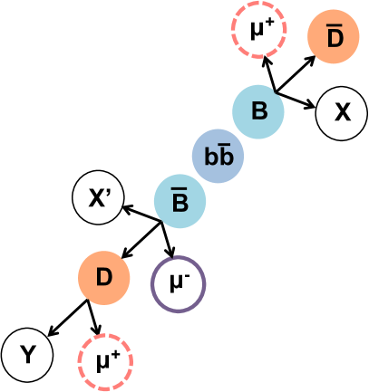
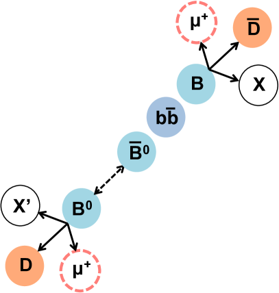
Figure 1: Like-sign muon pairs from bottom may arise from a combination of $B\rightarrow\mu$ and $B\rightarrow D\rightarrow\mu$ decay chains or from decays following $B^{0}\bar{B^{0}}$ oscillations .

At midrapidity the $e^{+}e^{-}$ pair continuum is dominated by pairs from heavy flavor decays in the measurable range from 1 to 15 GeV/$c^{2}$ Adare et al. (2017a), and thus having established the $b\bar{b}$ contribution would be sufficient to extract the $c\bar{c}$ cross section. However, at forward rapidity, $\mu^{+}\mu^{-}$ pairs from Drell-Yan can not be neglected. The Drell-Yan process involves quark-antiquark annihilation Drell and Yan (1970), whereas heavy flavor production is dominated by gluon fusion Norrbin and Sjostrand (2000). Due to the relative large Bjorken-$x$ of valence quarks compared to gluons, at forward rapidity the $\mu\mu$ pair yield above a mass of 6 GeV/$c^{2}$ is dominated by pairs from the Drell-Yan process. Thus, the Drell-Yan contribution can be determined from $\mu^{+}\mu^{-}$ pairs at high masses.

Once the contributions from $b\bar{b}$ decays and Drell-Yan production are constrained, the yield from $c\bar{c}$ can be measured in the mass range from 1 to 3 GeV/$c^{2}$, where it is significant, but only one of multiple contributions to the total yield in the mass range.

The paper is organized as follows: Sec. II outlines the experimental apparatus and the relevant triggers. Sec. III describes the procedure to extract muon pairs from the data. The expected $\mu\mu$ pair sources are discussed in Sec. IV. The Monte Carlo simulation used to generate templates for $\mu\mu$ pair spectra from the expected sources, which can be compared to the data, are presented in Sec. V. In Sec. VI we document the iterative template fitting method used to determine $c\bar{c}$, $b\bar{b}$ and Drell-Yan cross sections. Sec. VII discusses the sources of systematic uncertainties. The results are presented in Sec. VIII and finally we summarize our findings in Sec. X.

II Experimental Setup

The PHENIX detector comprises two central arms at midrapidity and two muon arms at forward and backward rapidity Adcox et al. (2003). The configuration of the experiment used for data taking with $p$+$p$ collisions in 2015 is shown in Fig. 2. Two muon spectrometers cover $\Delta\phi=2\pi$ in azimuth and $-2.2<\eta<-1.2$ (south arm) and $1.2<\eta<2.4$ (north arm) in pseudorapidity. The central arms are not used in this analysis.

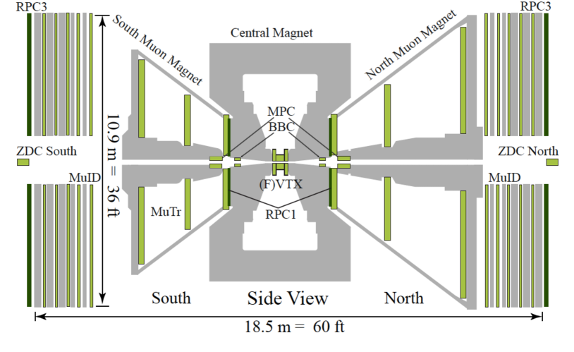
Figure 2: Side view of the PHENIX detector in the 2015 run.

Each muon arm comprises a forward-silicon vertex tracker (FVTX), followed by a hadron absorber with a muon spectrometer behind it. The spectrometer is composed of a charged particle tracker (MuTr) inside a magnet and a muon identification system (MuID). The FVTX allows for precision tracking, but has limited acceptance and is thus not used in this analysis.

The hadron absorber is composed of layers of copper, iron, and stainless steel, corresponding to a total of 7.2 interaction lengths ($\lambda_{I}$). The absorber suppresses muons from pion and kaon decays by about a factor of 1000, as it absorbs most pions and kaons before they decay. A small fraction of pions and kaons decays before they reach the absorber, which starts about 40 cm away from the nominal interaction point.

The MuTr has three stations of cathode strip chambers and provides a momentum measurement for the charged particles remaining after the absorber. The MuID is comprised of five alternating planes of steel absorbers [$4.8~{}(5.4)~{}\lambda_{I}$ for south (north) arm] and Iarocci tubes (gap 0–gap 4). The MuID provides identification of charged-particle trajectories based on the penetration depth. Only muons with momentum larger than 3 GeV/$c$ can penetrate all layers of absorbers. Signals in multiple MuID planes are combined to MuID tracks, which are used in the PHENIX trigger system to preselect events containing muon candidates. The trigger used to select the event sample for this analysis is a pair trigger (MuIDLL1-2D). For muon pairs with tracks that do not overlap in the MuID the MuIDLL1-2D is fired if both tracks independently fulfill the single track trigger requirement (MuDLL1-1D), which requires that the MuID track has at least one hit in the last two planes. A more detailed description of the PHENIX muon arms can be found in Ref. Akikawa et al. (2003).

The beam-beam counters (BBC) Allen et al. (2003) comprise two arrays of 64 quartz Čerenkov detectors located at $z=\pm 144~{}{\rm cm}$ from the nominal interaction point. Each BBC covers the full azimuth and the pseudorapidity range $3.1<|\eta|<3.9$. The BBCs are used to determine the collision-vertex position along the beam axis ($z_{\rm vtx}$) with a resolution of roughly 2 cm in $p$+$p$ collisions. The BBCs information also provides a minimum-bias (MB) trigger, which requires a coincidence between both sides with at least one hit on each side. The cross section of inelastic $p$+$p$ collisions at $\sqrt{s}=200$ GeV measured by the BBC, which is determined via the van der Meer scan technique Drees et al. (2003) ($\sigma^{p+p}_{\rm BBC}$), is $23.0{\pm}2.2$ mb.

III Data Analysis

III.1 Data set and event selection

The data set analyzed here was taken with $p$+$p$ collisions at $\sqrt{s}=200$ GeV in 2015. The data were selected with the $\mu\mu$ pair trigger (MuIDLL1-2D) in coincidence with the MB trigger. Each event in the sample has a reconstructed vertex within $z=\pm 30$ cm of the nominal collision point. The data sample corresponds to $1.2\times 10^{12}$ MB events or to an integrated luminosity of $\int\mathcal{L}dt=51$ pb^-1.

III.2 Track reconstruction

Each reconstructed muon track comprises a combination of a reconstructed tracklet in the MuTr and in the MuID. A number of quality cuts are applied to reduce the number of background muons from light hadron decays. They are summarized in Tab. 1. The tracklet in the MuTr must have a minimum of 11 hits and a $\chi^{2}/NDF$ smaller than 15 (20) for the south (north) arm. The MuID tracklet has to penetrate to the last gap and must have at least 5 associated hits. MuID tracklets with $\chi^{2}/NDF$ larger than 5 are rejected. MuTr tracklets are projected to MuID gap 0. We apply cuts on the distance between the projection of the MuTr tracklet and the MuID tracklet (DG0) and the difference between the track angles (DDG0). Figure 3 depicts DG0 and DDG0 distributions for muons with momenta of 4 to 5 GeV/$c$ from $\mu\mu$ pairs in the mass region 2.8–3.4 GeV/$c^{2}$ where $\mu\mu$ pairs from $J/\psi$ dominate the yield. Both distributions are compared to tracks from simulated $J/\psi$ decays. These cut variables are well described by simulations. We apply a cut at 3$\sigma$ ($99.87\%$ efficiency) of the momentum dependent matching resolution of signal tracks determined from Monte Carlo simulations with geant4 Agostinelli et al. (2003).

In addition to the basic track quality cuts, we enforce that the momentum of all reconstructed muon tracks are within $3<p$ [GeV/$c]<20$ and that their rapidity to be $1.2<|\eta|<2.2$. These requirements limit effects from detector acceptance edges. The upper limit on $p$ removes tracks from hadronic decays within the MuTr volume that lead to a mis-reconstructed momentum. We also require that all tracks satisfy the MuIDLL1-1D trigger condition.

While traversing the hadron absorber muons undergo multiple scattering and lose typically $2$ GeV of their energy before they reach the MuTr, where the momentum of the track is determined. Thus, the momentum needs to be corrected to correspond to the momentum in front of the absorber. The relative resolution has two main components, the intrinsic resolution of the MuTr and the resolution of the energy loss correction. Below 10 GeV/$c$ the resolution depends only moderately on rapidity or momentum and is approximately constant between 3.5 and 5%. Towards larger momenta it gradually increases but remains below 10% for all momenta considered in this analysis ($p<20$ GeV/$c$). Multiple scattering in the absorber adds an uncertainty of 160 mrad on the angular measurement from the MuTr. This can be vastly improved with the FVTX, which measures the track in front of the absorber. However, as discussed in the following section we do not make use of this improvement in the current analysis.

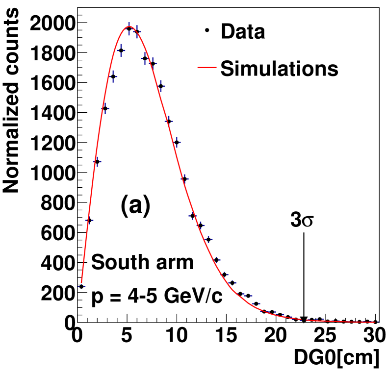
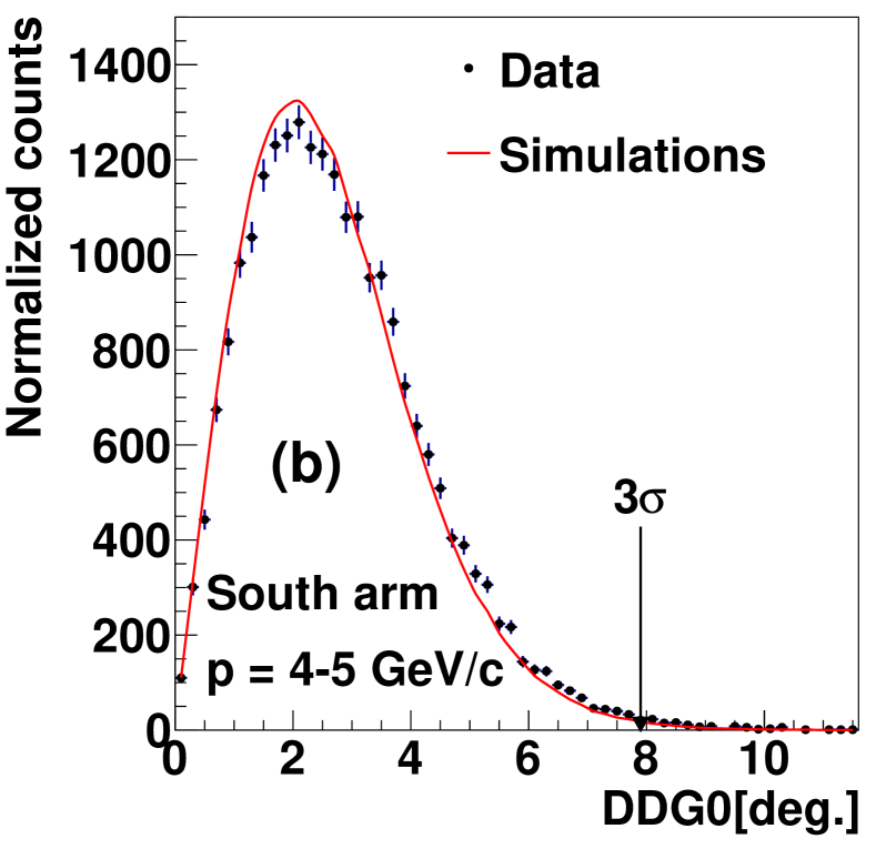
Figure 3: Matching of MuTr to MuID tracklets in distance (DG0) and angle (DDG0) for tracks from pairs in the $J/\psi$ mass region. Data and simulations are compared. The $3\sigma$ cut applied in the data analysis is indicated.

III.3 Muon pair selection

All muon tracks in a given event are combined to pairs and their masses and momenta are calculated. The mass is calculated from a fit to the two tracks with the constraint that both originate at a common vertex within the range $\pm 40$ cm around the nominal event vertex. This fitting procedure improves the resolution of the opening angle of the pair, which in turn significantly improves the mass resolution at $m<3$ GeV/$c^{2}$ where the mass resolution is dominated by effects from multiple scattering. We achieve a mass resolution $\sigma_{m}/m\approx 12.6\%,~{}7.4\%,~{}5.7\%$ at $m=1.02,~{}3.10,~{}9.46$ GeV/$c^{2}$ corresponding to the $\phi,~{}J/\psi$ and $\Upsilon(1S)$ respectively, which is sufficient for the analysis of the $\mu\mu$ pair continuum.

The mass resolution could be further improved by constraining the fit to the measured vertex position. However, our data set contains on average 22% of pileup events with two collisions recorded simultaneously. For these events only an average vertex position can be measured, which is often off by tens of centimeters from one or both of the collision points. This leads to $\mu\mu$ pair masses reconstructed hundreds of MeV/c² different from the true mass and results in a mass resolution function with significant non-Gaussian tails.

Figure 4(a) compares the mass distribution of the south muon arm and Fig. 4(b) for the north arm. The mass is calculated from the fits that constrain the tracks to originate from a vertex located at (i) $\pm 40$ cm of the nominal vertex (mass_nominal), and (ii) $\pm 2$ cm of the measured vertex using the BBC (mass_BBC). Although the width of the $J/\psi$ is narrower for mass_BBC as expected, the yield at the continuum on either sides of the $J/\psi$ is significantly different for the two mass calculations. To further diagnose this issue, we selected pairs with mass_BBC between 1.4 and 2.4 GeV/$c^{2}$ [panel (c)] and between 4.0 and 5.8 GeV/$c^{2}$ [panel (d)], and compared mass_BBC and mass_nominal distributions. In both mass_BBC selections, a clear $J/\psi$ peak is observed for mass_nominal, which indicates that the mass_BBC continuum contains a significant fraction of mis-reconstructed $J/\psi$ mesons, where the mis-reconstructed mass is due to a mis-measured vertex using the BBC in pileup events. To avoid this undesirable complication of the analysis of the $\mu\mu$ pair continuum, we do not make use of the improvement of the mass resolution. The pileup events increase the yield of $\mu\mu$ pairs per event by about 10%, this is taken into account in the normalization procedure.

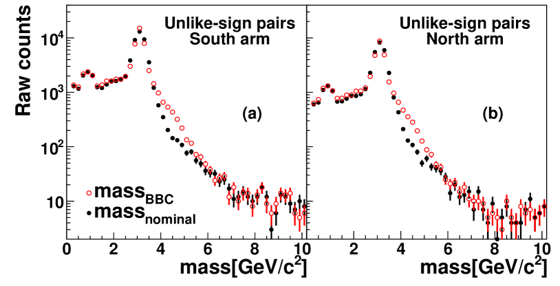
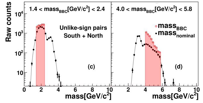
Figure 4: The mass spectra from the (a) south and (b) north arms, where the mass is calculated with different constraints to the vertex position: (i) a common vertex within $\pm 40$ cm around the nominal event vertex (mass_nominal, closed circles), and (ii) the vertex measured by the BBC (mass_BBC, open circles). mass_BBC and mass_nominal distributions are compared with pairs selected with mass_BBC (c) between 1.4 and 2.4 GeV/$c^{2}$, and (d) between 4.0 and 5.8 GeV/$c^{2}$.

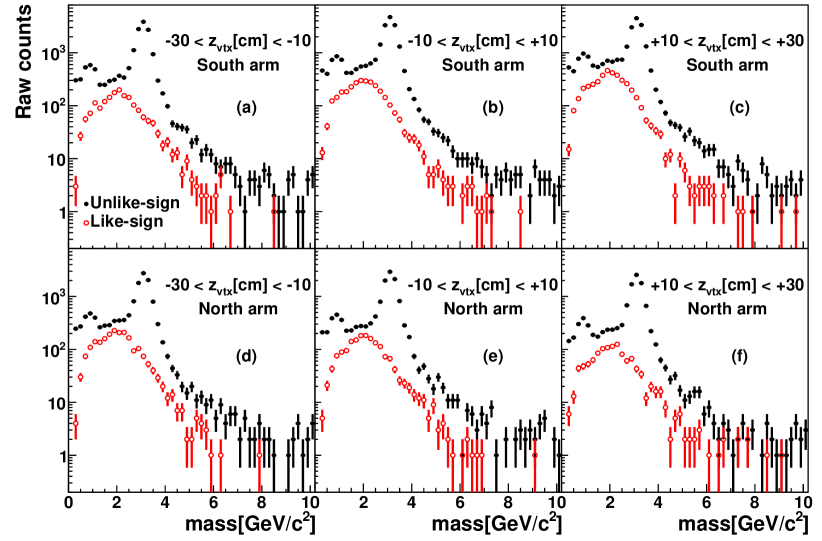
Figure 5: Raw mass spectra for the south and north muon arms in different $z_{\rm vtx}$ slices.

We apply additional quality cuts to the muon pairs, which are summarized in Table 2. The $\chi^{2}_{\rm vtx}$, computed from the simultaneous fit of the two muon tracks, must be less than 5. This cut mainly removes tracks that were either scattered by large angles in the absorber or that resulted from light hadron decays. We also remove pairs with a momentum asymmetry ($|p_{1}-p_{2}|/|p_{1}+p_{2}|$) larger than 0.55 because these pairs are mostly from random pairs where one hadron has decayed into a muon inside the MuTr and is mis-reconstructed as a higher momentum track, thus yielding a fake high mass pair.

Finally, we impose cuts to ensure spatial separation between two tracks in the MuTr and MuID volumes. Specifically we require that the vertical and horizontal spatial separation of the two tracks at the MuID gap 0 exceeds 20 cm. This cut removes all pairs with tracks that overlap so that for the remaining pairs the pair reconstruction and trigger efficiencies factorize into a product of single track efficiencies.

Table 1: Track quality cuts used in this analysis.

	south	north
Penetrate MuID last gap
MuTr $\chi^{2}$	$<15$	$<20$
Number of hits in MuTr	$>10$	$>10$
MuID $\chi^{2}$	$<5$	$<5$
Number of hits in MuID	$>5$	$>5$
${\rm DG0}(p)$	$<3\sigma$	$<3\sigma$
${\rm DDG0}(p)$	$<3\sigma$	$<3\sigma$

Table 2: Pair cuts used in this analysis.

$\chi^{2}_{\rm vtx}$	$<5$
$|p_{1}-p_{2}|/|p_{1}+p_{2}|$	$<0.55$
Muon pair do not share the same MuTr octant
$\Delta x$, $\Delta y$ at MuID gap 0	$>20$ cm

Figure 5 shows the raw mass spectra after imposing all single and pair cuts. Spectra are presented for $\mu^{+}\mu^{-}$ and $\mu^{\pm}\mu^{\pm}$ pairs measured for collisions in three vertex regions separately for the south and north arms.

The most prominent feature in the spectra is the $J/\psi$ peak at $\sim{3.1}$ GeV/$c^{2}$. For each arm the yield is independent of $z$ within 10%–20%. Pairs in the north arm are reconstructed with about 2/3 of the efficiency compared to the south arm, which is mostly due to a larger dead area in the north MuTr, but otherwise the spectra are similar for mirrored $z$ ranges. The like-sign spectra have the lowest yield for the $z$ range closest to the absorber, negative and positive $z$ for south and north arm, respectively. The $\mu^{\pm}\mu^{\pm}$ yield increases by roughly a factor of three as the collision point moves away from the absorber and more pions and kaons decay in flight before reaching the absorber.

IV Expected pair sources

To interpret the experimental data shown in Fig. 5, we need to compare it to the $\mu\mu$ pairs from known sources, commonly referred to as “cocktail”. Besides our signal of interest, $\mu\mu$ pairs from open heavy flavor (semi-leptonic decays of $c\bar{c}$ and $b\bar{b}$) and Drell-Yan, the cocktail contains large contributions from hadron (pseudoscalar and vector meson) decays, and unphysical background pairs. The quantitative comparison is done through template $\mu\mu$ pair distributions that are generated for the individual known sources.

The unphysical background pairs typically involve muons from the decays of light hadrons ($\pi^{\pm}$, $K^{\pm}$, and $K^{0}$). The production rates of decay muon from light hadrons overwhelm those of signal muons from $c\bar{c}$, $b\bar{b}$, and Drell-Yan. Therefore, in spite of the large hadron rejection power ($\sim 1/1000$) of the muon arms, a substantial fraction of the reconstructed muons are from pion and kaon decays that occur before they reach the absorber. Because the distance to the absorber varies from 10 to 70 cm, depending on the $z$ location of the event vertex $z_{\rm vtx}$, the unphysical background varies significantly with $z_{\rm vtx}$. A smaller, but non negligible fraction of background tracks are hadrons that penetrate all layers of absorber and are therefore reconstructed as muon candidates. In addition, hadrons can interact strongly with the absorber to produce showers of secondary particles, which can also be reconstructed as muon candidates. Pairs including at least one of these so called hadronic tracks, i.e. a muon from light hadron decay, a punch-through hadron or a secondary particle from hadronic showers, are a large contribution to the measured $\mu\mu$ pairs.

In the following subsections we discuss how we can generate the known sources of $\mu\mu$ pairs, which are needed as input for the templates of $\mu\mu$ pair spectra used in the subsequent analysis.

IV.1 Physical $\mu\mu$ pair sources

IV.1.1 Hadron decays to $\mu\mu$ pairs ($h\rightarrow\mu\mu(X)$)

Decays from $\eta$, $\eta^{\prime}$, $\omega$, $\rho$, and $\phi$ dominate the $\mu^{+}\mu^{-}$ pair yield below a mass of 1 GeV/$c^{2}$, whereas decays from $J/\psi$, $\psi^{\prime}$, and $\Upsilon(1S+2S+3S)$ dominate the $\mu^{+}\mu^{-}$ pair yield in narrow mass regions at higher masses. We use existing data to constrain the input distributions for these mesons whenever possible.

The mesons $\rho$, $\omega$, $\phi$, and $J/\psi$ can be generated based on the measured differential cross sections Adare et al. (2012, 2014b) that are displayed on in Fig. 6(c). We use the Gounaris/Sakurai parameterization to describe the line shape of the $\rho$ meson mass distribution Gounaris and Sakurai (1968). The $\rho$ is fixed to the $\omega$ with $\sigma_{\rho}/\sigma_{\omega}=1.21\pm 0.13$, which is consistent with the value found in jet fragmentation Patrignani et al. (2016). Because there is no measurement at forward rapidity, we constrain the $\eta$ and $\eta^{\prime}$ using measurements at midrapidity Adler et al. (2007a); Adare et al. (2011b, c), which is shown in Fig. 6(a), and use pythia v6.428 Sjostrand et al. to extrapolate to forward rapidity.

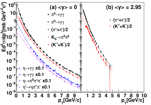
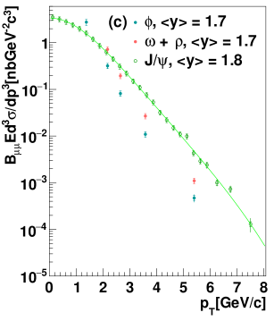
Figure 6: Compilation of meson production in $p$+$p$ collisions at $\sqrt{s}=200$ GeV at (a) $\langle y\rangle=0$, (b) $\langle y\rangle=2.95$ and (c) $\langle y\rangle=1.7$–1.8. The data at $\langle y\rangle=0$ is taken from PHENIX: $\pi^{0}\rightarrow\gamma\gamma$ Adare et al. (2007)(black star),Adler et al. (2003)(black open circle), $(\pi^{+}+\pi^{-})/2$ Adare et al. (2011d), $K_{S}\rightarrow\pi^{0}\pi^{0}$ Adare et al. (2011b), $(K^{+}+K^{-})/2$ Adare et al. (2011d), $\eta\rightarrow\gamma\gamma$ Adler et al. (2007a)(blue star),Adare et al. (2011c)(blue open circle), $\eta\rightarrow\pi^{0}\pi^{+}\pi^{-}$ Adler et al. (2007a), $\eta^{\prime}\rightarrow\eta\pi^{+}\pi^{-}$ Adare et al. (2011b). The data at $\langle y\rangle=2.95$ is taken from BRAHMS: $(\pi^{+}+\pi^{-})/2$ Arsene et al. (2007), $(K^{+}+K^{-})/2$ Arsene et al. (2007). The data at $\langle y\rangle=1.7$–1.8 is taken from PHENIX: $\phi\rightarrow\mu\mu$ Adare et al. (2014b), $\omega+\rho\rightarrow\mu\mu$ Adare et al. (2014b), $J/\psi\rightarrow\mu\mu$ Adare et al. (2012). The curves are fits using modified Hagedorn Adare et al. (2017a) or Tsallis Tsallis (1988) functions to data.

The $p_{T}$ spectra of $\psi^{\prime}$ and $\Upsilon$ are generated using pythia and normalized using the measurements of $\psi^{\prime}$ to $J/\psi$ ratio Adare et al. (2017b) and $B_{\mu\mu}dN_{\Upsilon}/dy$ Adare et al. (2013), respectively. All mesons are decayed using pythia to handle the decay kinematics.

IV.1.2 Open Heavy flavor

The $\mu\mu$ pairs that originate from semi-leptonic decays of heavy flavor hadrons, or heavy flavor pairs, are simulated using two event generators, pythia and powheg.

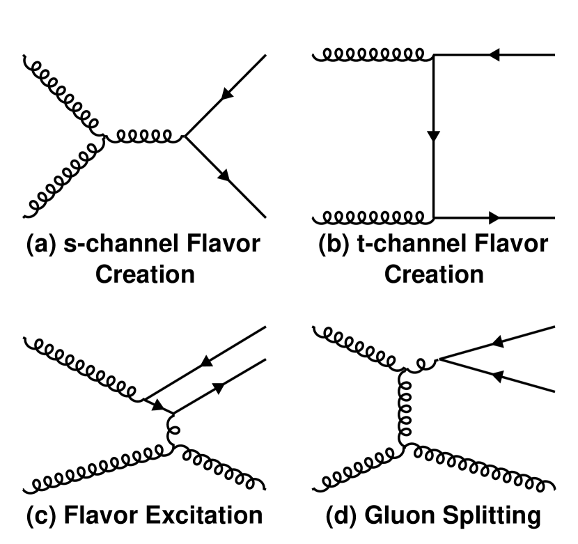
Figure 7: Feynman diagrams corresponding to flavor creation (a,b), flavor excitation (c) and gluon splitting (d) Norrbin and Sjostrand (2000); Ilten et al. (2017).

We use pythia version v6.428 Sjostrand et al. . We use Tune A input parameters as shown in Table 6 in Appendix C. In contrast to using the forced $c\bar{c}$ and $b\bar{b}$ production modes (MSEL4 or 5), which include only lowest-order process of flavor creation ($gg\to Q\bar{Q}$), we used the mode (MSEL1) which also simulates higher-order processes of flavor excitation ($gQ\to gQ$) and gluon splitting ($gg\to Q\bar{Q}g$). Figure 7 shows the Feynman diagrams corresponding to the different production processes. Leading order matrix elements are used for the initial hard process, and next-to-leading order corrections are implemented with a parton-shower approach. A classification of the three classes of processes can be achieved by tagging the event record which contains the full ancestry of any given particle; a detailed account of the characterization of these three classes can be found in Ref. Norrbin and Sjostrand (2000).

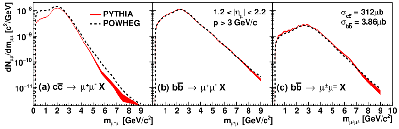
Figure 8: Comparison of $\mu\mu$ yield in the ideal muon arm acceptance determined using pythia (red solid) and powheg (black dotted). Both are normalized using cross sections($\sigma_{cc}=312\mu b$, $\sigma_{bb}=3.86\mu b$) from Adare et al. (2017a). The width of the pythia band represents the statistical uncertainty in the calculation.

We also use powheg version v1.0 Frixione et al. (a) interfaced with pythia v8.100 Sjostrand et al. (2008) to generate heavy flavor muon pairs. We use the default setting for $c\bar{c}$ and $b\bar{b}$ productions, including the choices for normalization and factorization scales and heavy quark masses. CTEQ6M is used for parton distribution functions of the proton. In contrast to pythia, NLO corrections are directly implemented in the hard process using next-to-leading order matrix elements. As such, the classification of processes in pythia is not applicable for powheg; there is no trivial connection between the classes of processes in the pythia formalism and the powheg formalism.

The simulated mass spectra of pairs in the ideal muon arm acceptance, which requires that each muon has a momentum $p>3$ GeV/$c$ and falls into the pseudorapidity range $1.2<|\eta|<2.2$, from $c\bar{c}$ and $b\bar{b}$ are shown in Fig. 8. Like-sign pairs from $c\bar{c}$ is found to be negligible compared to $b\bar{b}$ in the entire kinematic region and hence neglected for this analysis.

The $\mu^{+}\mu^{-}$ and $\mu^{\pm}\mu^{\pm}$ pair spectra from $b\bar{b}$ are very similar for both generators; this is consistent with the findings in Refs. Adare et al. (2015, 2017a) that, because of the large $b$-quark mass the spectra are dominated by decay kinematics rather than the correlation between the $b$ and $\bar{b}$ quarks. For the same reason variations of the scale and PDFs have a small effect on the shape of the mass spectra.

In contrast, we observe a significant model dependence for $\mu^{+}\mu^{-}$ pairs from $c\bar{c}$, indicating a much larger sensitivity to the correlation between the $c$ and $\bar{c}$ quarks. Similar to $e^{+}e^{-}$ pairs Adare et al. (2016), this is most pronounced at low masses. This is due to differences in description of the correlations between the $c$ and $\bar{c}$ quarks; the opening angle distributions in powheg is flatter which leads to higher yields at low masses. A smaller but non-negligible discrepancy at higher masses is also observed. Because high mass pairs are dominated by back-to-back pairs from leading order processes, this difference is likely due to a harder $p_{T}$ spectrum predicted by powheg compared to pythia.

IV.1.3 Drell-Yan

We use pythia v6.428 to simulate $\mu\mu$ pairs from the Drell-Yan production mechanism (Drell-Yan pairs). The input parameters are shown in Table 7 in Appendix C. The primordial $k_{T}$ is generated from a Gaussian distribution. The width of the distribution is $1.1$ GeV/$c$ and was determined by investigating the $p_{T}$ distribution of unlike-sign pairs in the mass region 4.8–8.6 GeV/$c^{2}$ where the yield is expected to be dominated by Drell-Yan Arnaldi et al. (2009). The procedure and its associated uncertainties will be explained in detail in Sec. VII.1.4.

IV.2 Unphysical $\mu\mu$ pair sources

Unphysical pair background is customarily subdivided into combinatorial and correlated pairs. Here the idea is that for combinatorial pairs the two tracks have no common origin and thus are uncorrelated. In contrast, for correlated pairs the tracks do have a common origin, for example they both stem from the decay chain of a heavy hadron or they were part of the fragmentation products of a jet or the like.

In $p$+$p$ collisions, or generally in events with a small number of produced particles, the distinction between combinatorial and correlated pairs is not well defined. A $p$+$p$ collision typically produces hard scattered partons accompanied by an underlying event, which consists of initial and final state radiation, beam-beam remnants and multiple parton interactions. The complex event structure in a single $p$+$p$ event forbids a clear identification of whether two particles stem from a common origin or not. All particles are produced from the two colliding protons, and thus are correlated through momentum and charge conservation. Therefore, the separation is more procedural and is defined by how the relative contributions of correlated and combinatorial pairs are determined. We use an approach that maximizes the number of pairs considered combinatorial, which will be discussed in detail in Sec. VI.1.2.

The individual contributions of the unphysical pair background are determined using Monte-Carlo event generators. We treat pairs that are made from two hadronic tracks (hadron-hadron pairs: $N_{hh}$) and those with one hadronic track and the other being a muon from the decay of a $D$, $B$, or $J/\psi$ meson (muon-hadron pairs: $N_{Dh}$, $N_{Bh}$ and $N_{Jh}$) separately.

IV.2.1 Hadron-hadron pairs: $N_{hh}$

The $N_{hh}$ pairs are simulated with pythia, using parameters listed in Table 6. This Tune A setup reproduces jet-like hadron-hadron correlations at midrapidity in $p$+$p$ collisions at $\sqrt{s}=200$ GeV Adler et al. (2006a) reasonably well. To also reproduce the $p_{T}$ spectra we use momentum dependent weighting to match the pythia distributions to data. In the literature there are no data for $p_{T}$ spectra of charged pions and kaons from $p$+$p$ collisions at $\sqrt{s}=$200 GeV in the rapidity region covered by the muon arms. Thus, we interpolate between $p_{T}$ spectra measured at midrapidity Adler et al. (2003); Adare et al. (2007, 2011d, 2011b) and very forward rapidity ($2.9<y<3.0$) Arsene et al. (2007). The data are given in Fig. 6. Weighting factors are extracted for both rapidity ranges as a function of $p_{T}$, by taking the ratio between data and pythia,

$$w_{h}(y=0,p_{T}) =\frac{E\frac{d^{3}\sigma}{dp^{3}}|_{y=0,DATA}}{E\frac{d^{3}\sigma}{dp^{3}}|_{y=0,PYTHIA}},$$ (1)

$$w_{h}(y=2.95,p_{T}) =\frac{E\frac{d^{3}\sigma}{dp^{3}}|_{y=2.95,DATA}}{E\frac{d^{3}\sigma}{dp^{3}}|_{y=2.95,PYTHIA}},$$ (2)

where $h$ stands for pion or kaon. For a given $p_{T}$, we linearly interpolate the weighting factors as a function of $y$:

$$w_{h}(y,p_{T})= \frac{y}{2.95}\times[w_{h}(y=2.95,p_{T})-w_{h}(y=0,p_{T})]$$

$$+w_{h}(y=0,p_{T}).$$ (3)

These weighting factors are shown in Fig. 9. Above $p_{T}$ = 5 GeV/$c$, where there are no data at forward rapidity, the weights are assumed to be constant. The systematic uncertainties from this weighting procedure are discussed in Sec. VII. The weighting factors are applied to each input particle generated with the pythia simulation.

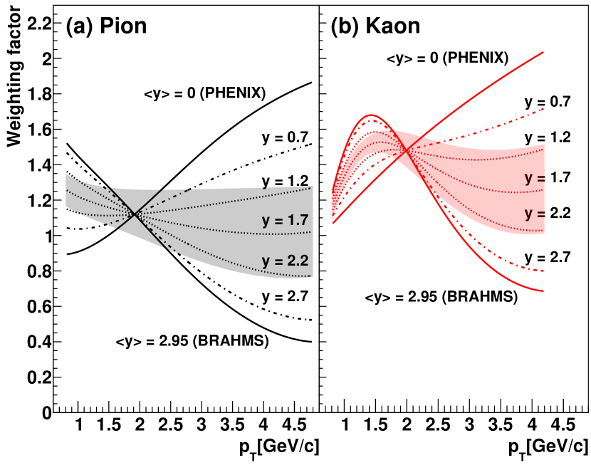
Figure 9: Weighting factors for (a) pions and (b) kaons in different rapidity slices. The shaded bands indicate uncertainty brackets used for the investigation of systematic uncertainties (see Sec. VII.1.1).

IV.2.2 Muon-hadron pairs: $N_{Dh}$, $N_{Bh}$, and $N_{Jh}$

Muon-hadron pairs $N_{Dh}$ and $N_{Bh}$ as defined above are constructed using the same pythia and powheg simulations that determine the open heavy flavor pair input. The pion and kaon $p_{T}$ spectra are tuned the same way as discussed above. For the muon-hadron pairs involving decays of the $J/\psi$ ($N_{Jh}$) we also match the pythia $J/\psi$ momentum spectrum at forward rapidity to reproduce the measured $J/\psi$-hadron yield per MB event Adare et al. (2012) (see Fig. 6).

IV.2.3 Combinatorial pair background

The combinatorial pair background is constructed via an event mixing technique, which combines tracks from different events of similar vertex position $z$. This is done separately for data and the events used to simulate hadron-hadron pairs, and muon-hadron pairs.

To optimize the description of the pair background spectrum, we maximize the contribution identified as combinatorial pair background, subtract the combinatorial component from the simulation of hadron-hadron and muon-hadron pairs, and substitute the combinatorial pair background with the one determined from data. The motivation of this procedure and the details of the normalization of individual components are discussed in Sec. VI.1.

V Simulation framework

To directly compare the expected sources to the data, the $\mu\mu$ pairs from the expected sources are propagated through a Monte-Carlo simulation of the PHENIX detector. This simulation is designed to emulate in detail the detector response, and the recording and analysis of data taken with the PHENIX experiment. Histograms of the expected number of $\mu\mu$ pairs are constructed in mass-$p_{T}$ bins, which serve as templates for the subsequent fitting procedure.

The $\mu\mu$ pairs from all physical sources are propagated through the default PHENIX simulation framework. The same approach is not practical for unphysical pair background from $\pi$ and $K$ decays. Because of the large ($\sim$1/1000) rejection power for these backgrounds, an undesirably large amount of simulations would be necessary to reach sufficient statistical accuracy. Therefore, we use a fast Monte-Carlo (FastMC), developed specifically for this analysis. Detailed descriptions of the two simulation chains can be found in Appendix A.

VI Iterative procedure to extract charm, bottom and Drell-Yan cross sections

In the previous two sections we have discussed the different expected sources of $\mu\mu$ pairs and how template distribution of $\mu\mu$ pairs are generated for each. In this section we compare the templates for the expected sources to the experimental data and determine the absolute contribution of each source.

After an initial normalization is chosen for each template, the key sources, $c\bar{c}$, $b\bar{b}$, Drell-Yan, and the hadronic pair background, are normalized in an iterative template fitting procedure.

VI.1 Initial normalization and data-driven tuning of cocktail

VI.1.1 Physical $\mu\mu$ pair sources

The normalization of muon pairs from hadron decays $h\rightarrow\mu\mu(X)$ is fixed because the cross sections of the parent mesons are set by experimental data as discussed in Sec. IV.1.1. The normalizations for each component are varied separate within experimental uncertainties to estimate the corresponding systematic uncertainties (see Sec. VII).

The distributions for muon pairs from $c\bar{c}$, $b\bar{b}$, and Drell-Yan are normalized by the parameters $\kappa_{c\bar{c}}$, $\kappa_{b\bar{b}}$, and $\kappa_{\rm DY}$. These parameters will be determined via the iterative fitting procedure presented in this section. The initial values of $\kappa_{c\bar{c}}$, $\kappa_{b\bar{b}}$, and $\kappa_{\rm DY}$ are set based on measured data Adare et al. (2017a).

VI.1.2 Correlated hadrons and combinatorial pair background

The composition and normalization of the unphysical pair background sources is key to understanding the $\mu\mu$ continuum and requires a more detailed discussion. In $p$+$p$ collisions at $\sqrt{s}=200$ GeV, the multiplicity of produced particles is low, and hence there is no clear-cut method to differentiate between a correlated pair and a combinatorial pair. Great care is taken to assure that the procedure used to define combinatorial pairs and how their contribution is normalized does not affect the extraction of physical quantities.

One possibility to circumvent the distinction of correlated and combinatorial pairs is to generate hadron-hadron and muon-hadron pairs using a Monte-Carlo event generator like pythia interfaced to the FastMC framework. Templates from a full event normalization include all background pair sources, hence the distinction between them is not necessary. However, in this method the extracted physical cross section is sensitive to how accurate pythia describes the underlying event and how well geant4 treats hadronic interactions in the absorber. This may increase the systematic uncertainties on the extraction of the $c\bar{c}$, $b\bar{b}$, and Drell-Yan components.

In this analysis we use a data-driven hybrid approach, in which

• the maximum possible number of combinatorial pairs is determined from the generated pythia and/or powheg events,

• the correlated hadronic pairs are calculated by subtracting the combinatorial pairs determined by mixing generated events,

• the combinatorial pairs are replaced by the combinatorial pairs determined from data.

Although the distinction between correlated hadronic pairs and combinatorial pairs depends on the choice of the normalization procedure, using different procedures has a negligible effect on extraction of physical cross sections. The separation of these two components is mostly important for the evaluation of systematic uncertainties, because the correlated hadronic pairs depend on simulations and the combinatorial pairs do not. Replacing the combinatorial pairs from the generator with mixed pairs from data should be regarded as a correction to the simulations to reduce systematic uncertainties.

Normalizing hadron-hadron and muon-hadron pairs

The templates for hadron-hadron pairs $N_{hh}(m,p_{T},z)$ are generated using pythia simulations interfaced to the FastMC, as discussed above. Templates are determined separately for the three different $z$ regions ($z^{\prime}_{i}$) available in the FastMC simulations, $z^{\prime}_{0}=(-22.5,-17.5~{}{\rm cm})$, $z^{\prime}_{1}=(-2.5,+2.5~{}{\rm cm})$ and $z^{\prime}_{2}=(+17.5,+22.5~{}{\rm cm})$, respectively. Only pions, kaons, and their decay products are considered. The momentum spectra were tuned to accurately describe experimental data, where available (see Sec. IV.2.1). Therefore, $N_{hh}$ contains the correct mix of individual hadron-hadron pair sources per event. $N_{hh}$ is initially normalized as a per event yield for generated MB $p$+$p$ collisions.

Similarly, muon-hadron pair templates from $c\bar{c}$ and $b\bar{b}$ are constructed using pythia and powheg generators interfaced to the FastMC. The templates $N_{Dh}(m,p_{T},z)$ and $N_{Bh}(m,p_{T},z)$ correspond to muon-hadron pairs from $c\bar{c}$ and $b\bar{b}$, respectively. Each is normalized per $c\bar{c}$ or $b\bar{b}$ event. Thus, they can be added to $N_{hh}$ scaled by the normalization factors $\kappa_{c\bar{c}}$ and $\kappa_{b\bar{b}}$, used for the $\mu\mu$ pairs, such that $\kappa_{c\bar{c}}N_{Dh}$ and $\kappa_{b\bar{b}}N_{Bh}$ are the expected muon-hadron pair yields per MB $p$+$p$ event.

For $J/\psi$, the differential cross section at forward rapidity has been measured Adare et al. (2012). Analogous to the pion and kaon simulations, we weight the simulated $J/\psi$ momentum distribution to match the $J/\psi$ yield at forward rapidity. Because the simulated $J/\psi$ yield is normalized to the measured yield, the muon-hadron pair template $N_{Jh}(m,p_{T},z)$ represents a yield per MB $p$+$p$ event.

The full per MB $p$+$p$ event hadronic pair background can thus be written as:

$$N_{hbg}=\kappa_{c\bar{c}}N_{Dh}+\kappa_{b\bar{b}}N_{Bh}+N_{hh}+N_{Jh},$$ (4)

where the templates are functions of $m$, $p_{T}$, and $z$. Figure 10(a) shows $N_{hbg}$ and its individual contributions integrated over $z$ and $p_{T}$ as a function of mass.

Choice and normalization of the combinatorial pair background

To minimize any remaining model dependence in $N_{hbg}$ used in the analysis, we determine the combinatorial contribution to $N_{hbg}$ from mixed generated events and replace it with the combinatorial pairs determined from data. For each simulation we determine the combinatorial pairs by mixing either hadron-hadron pairs or muon-hadron pairs from different events at the same $z^{\prime}_{i}$. For a given $z^{\prime}_{i}$ bin the combinatorial pairs are then constructed as:

$$N_{\rm comb,sim}=\kappa_{c\bar{c}}N_{Dh}^{\rm mix}+\kappa_{b\bar{b}}N_{Bh}^{\rm mix}+N_{hh}^{\rm mix}+N_{Jh}^{\rm mix},$$ (5)

which observes the same relative normalization of the individual components as in Eq. 4. The contributions of each component to the hadronic and the combinatorial pair background, normalized following the above procedure are shown in Fig. 10(b).

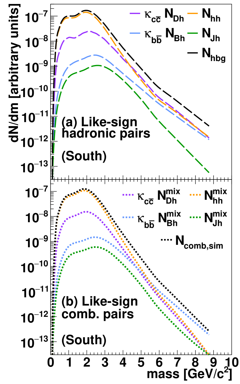
Figure 10: (a) full simulation for hadronic pairs and (b) combinatorial pairs for mass spectra of hadron-hadron and muon-hadron pairs from charm, bottom and $J/\psi$ after initial normalization and tuning.

The normalization of the combinatorial pairs is determined statistically via the ZYAM (Zero Yield At Minimum) technique Adler et al. (2006b) as described below. We use the azimuthal angle difference $\Delta\phi_{prim}$ of the like-sign hadronic pairs with masses less than 3 GeV/$c^{2}$. Here $\Delta\phi_{prim}$ is the difference of the azimuthal angles of the input particles ($\pi$, $K$, $D$, or $B$); the distribution is shown in Fig. 11.

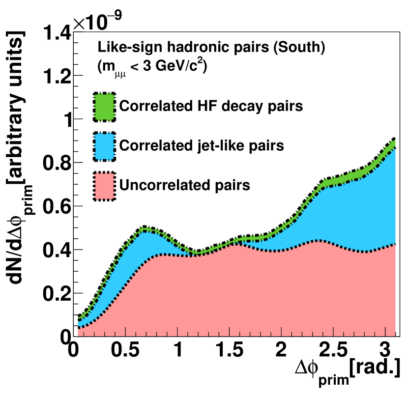
Figure 11: ZYAM normalization procedure for the south muon arm. The normalization of the uncorrelated pairs from event mixing (red) is determined by enforcing the requirement that the yield of the uncorrelated pairs ($N_{\rm corr,sim}$) is identical to the yield of foreground pairs ($N_{hbg}$), excluding the pairs from heavy-flavor decay chains (green) at $\Delta\phi_{prim}\sim\pi/2$. The excess yield is from away-side and near-side jet-like correlations (blue). The periodicity of the distributions arises from the octant structure of the MuTr.

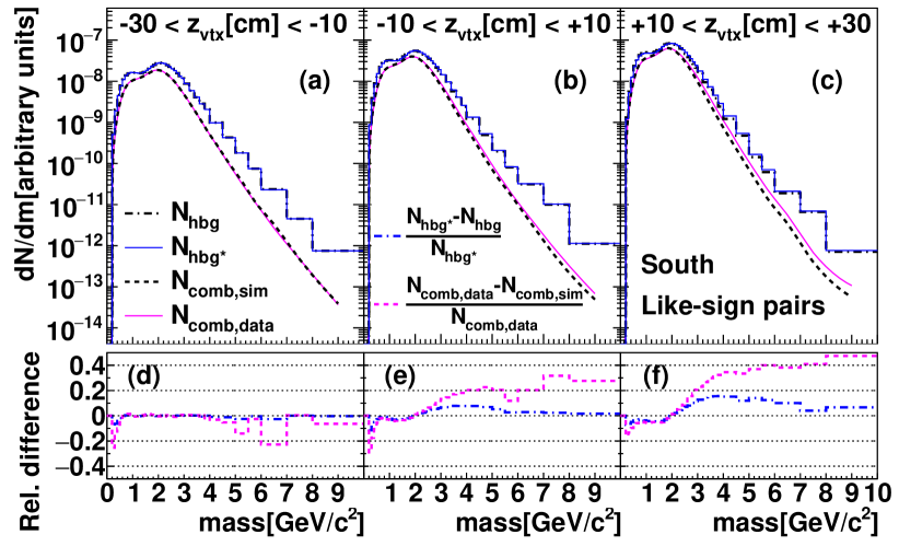
Figure 12: Like-sign mass spectra of the hadronic pair background (before and after correction by replacing with combinatorial pairs from data), and combinatorial background (simulations and data) in different $z_{\rm vtx}$ regions. Panels (d,e,f) show the relative difference between different mass spectra.

First, we remove muon-hadron pairs in which both tracks originated from heavy flavor ($c\bar{c}$ or $b\bar{b}$) pairs, because these pairs can uniquely be identified as correlated. For the remaining pairs we assume that correlations result mostly from jet-fragmentation. These should have a minimal contribution for $\Delta\phi_{prim}\sim\pi/2$. Thus, our ZYAM assumption is that the correlated yield vanishes at $\Delta\phi_{prim}=\pi/2$. The excess yield for $\Delta\phi_{prim}<\pi/2$ can be interpreted as pairs from the same jet, whereas the excess yield for $\Delta\phi_{prim}>\pi/2$ would correspond to $\mu\mu$ pairs from back-to-back jets. The correlated $N_{\rm corr,sim}$ and combinatorial $N_{\rm comb,sim}$ contributions are now separated via the relations:

$$N_{\rm corr,sim} =N_{hbg}-N_{\rm comb,sim}.$$ (6)

The separation of $N_{hbg}$ into correlated and uncorrelated components is done for each of the three vertex region $z^{\prime}_{i}$ used in the FastMC simulations. In the data, mixed events are also constructed in 5 cm $z$-bins, but over the full range from -30 cm to 30 cm. The template distributions are aggregated for three broad vertex ranges, $z_{0}=(-30,-10~{}{\rm cm})$, $z_{1}=(-10,+10~{}{\rm cm})$ and $z_{2}=(+10,+30~{}{\rm cm})$. The normalization of the mixed events from the data is matched to those from the simulation by scaling $N_{hbg}(z^{\prime}_{i})$ such that the number of combinatorial pairs of data and simulations are identical in the normalization mass region $\mathcal{M}$ ($m<3$GeV/$c^{2}$) for each $z$ bin, i.e., we require:

$$\int\limits_{\mathcal{M}}N_{\rm comb,sim}(z^{\prime}_{i})=\int\limits_{\mathcal{M}}N_{\rm comb,data}(z_{i})$$ (7)

This rescaling is necessary because we are approximating a $\Delta z_{i}$ range of 20 cm from data with a $\Delta z_{i}^{\prime}$ range of 5 cm from simulations. For the two $z$ bins further away from the absorber, this approximation holds well even without rescaling because the multiplicity falls linearly with the distance from the absorber, and the center of the bin times the bin width is to first order a good approximation of the integral of the bin. However, for the $z$ bin closest to the absorber, this linear relation no longer holds and a scaling factor of $1.2$ is applied to $N_{\rm comb,sim}$ according to Eq. 7.

We then replace the combinatorial background from simulations by data for each vertex region $z_{i}$:

$$N_{hbg*}(z_{i})=N_{\rm corr,sim}(z^{\prime}_{i})+N_{\rm comb,data}(z_{i}).$$ (8)

The hadronic pair background in each vertex slice for the south arm, before and after the above replacement of the combinatorial pair background, is shown in Fig. 12. The relative mass-dependent difference between the two estimates of the hadronic pair background ranges from $\sim 0\%$ for the $z_{\rm vtx}$ region closest to the absorber to a maximum of $\sim 20\%$ at $m\sim 4$ GeV/$c^{2}$ for the z_vtx region furthest away from the absorber.

The same normalization is applied to unlike-sign hadronic pairs. Both the unlike- and like-sign hadronic pairs are scaled with a common normalization factor $\kappa_{h}$ to be determined in the fitting procedure. Finally, we define the correlated hadronic pairs, $N_{\rm cor}$ and combinatorial pairs, $N_{\rm comb}$ via the relations:

$$N_{\rm cor} =N_{\rm corr,sim},$$

$$N_{\rm comb} =N_{\rm comb,data}.$$ (9)

The distinction between correlated and combinatorial hadronic pairs depends on the details of the normalization procedure. Different normalization procedures can lead to significant differences in the relative contributions of correlated and combinatorial components. However, the effect on the extraction of physical cross sections is small. The variations are included in the systematic uncertainties (see Sec. VII.1.5).

VI.2 Iterative fit

Fit strategy

The absolute contribution of each of the various known sources to the $\mu^{+}\mu^{-}$ and $\mu^{\pm}\mu^{\pm}$ spectra is determined by a fitting procedure using a template distribution for each contribution. There are four fit parameters, $\kappa_{c\bar{c}}$, $\kappa_{b\bar{b}}$, $\kappa_{\rm DY}$, and $\kappa_{h}$, which are normalization factors for the contributions from $c\bar{c}$, $b\bar{b}$, Drell-Yan, and the hadronic pairs.

We adopt the following iterative fitting strategy, here parameters marked with a tilde correspond to fit values obtained in the previous step:

1. With a fixed $\kappa_{c\bar{c}}$, fit the like-sign spectrum with $\kappa_{b\bar{b}}$ and $\kappa_{h}$ as free parameters in mass-$p_{T}$-$z_{\rm vtx}$ slices in the mass range 1–10 GeV/$c^{2}$.

2. With the same $\kappa_{c\bar{c}}$ as in step (i) and $\tilde{\kappa}_{b\bar{b}}$ and $\tilde{\kappa}_{h}$ obtained in (i), fit mass and $p_{T}$ slices in the unlike-sign mass region 4.4–8.5 GeV/$c^{2}$ with $\kappa_{\rm DY}$ as a free parameter.

3. With $\tilde{\kappa}_{b\bar{b}}$ and $\tilde{\kappa}_{h}$ obtained in (i) and $\tilde{\kappa}_{\rm DY}$ in (ii), fit mass and $p_{T}$ slices in the unlike-sign mass region 1.4–2.5 GeV/$c^{2}$ with $p_{T}<2$ GeV/$c$, with $\kappa_{c\bar{c}}$ as a free parameter.

4. Iterate with $\tilde{\kappa}_{c\bar{c}}$ from (iii).

This method of fitting exploits the fact that the like-sign pairs contain mainly contributions from hadronic pairs and $b\bar{b}$; charm only contributes via muon-hadron pairs and is non-dominant while Drell-Yan does not contribute. Thus, the fit results in step (i) is not sensitive to the initial starting value of $\kappa_{c\bar{c}}$. The contribution of hadronic pairs to the $\mu^{+}\mu^{-}$ and $\mu^{\pm}\mu^{\pm}$ pairs increases as the distance between the event vertex $z_{\rm vtx}$ and the absorber becomes larger, due to enhanced probability of pions and kaons to decay before they hit the absorber. In contrast, the yield of $\mu\mu$ pairs from $b\bar{b}$ is independent of $z_{\rm vtx}$. To optimize the separating power between $\mu\mu$ pairs from $b\bar{b}$ and the hadronic pairs, in step (i) we fit like-sign pairs in mass-$p_{T}$-$z_{\rm vtx}$ slices. Step (i) gives strong constraints on $\kappa_{b\bar{b}}$ and $\kappa_{h}$, which are to first order free from systematic uncertainties on the $c\bar{c}$ and Drell-Yan templates. With $\kappa_{b\bar{b}}$ and $\kappa_{h}$ constrained, we move on to step (ii), where we fit the unlike-sign pairs with mass 4.4–8.5 GeV/$c^{2}$. This mass region is chosen to avoid contributions from quarkonia decays. Here, Drell-Yan and $b\bar{b}$ contributions are expected to dominate while contributions from $c\bar{c}$ and hadrons are secondary. Although Drell-Yan also contributes to lower masses, the sensitivity to the intrinsic $k_{T}$ make it unfavorable to constrain $\kappa_{\rm DY}$ in the low mass region. With $\kappa_{b\bar{b}}$, $\kappa_{h}$ and $\kappa_{\rm DY}$ constrained, we fit in the mass region 1.4–2.5 GeV/$c^{2}$ to constrain $\kappa_{c\bar{c}}$. This mass region is chosen to minimize the contributions of decays from quarkonia and low mass mesons. In this step, we exclude the region with $p_{T}>2$ GeV/$c$ from the $\mu^{+}\mu^{-}$ spectra from the fit, to avoid the uncertainty of the shape of Drell-Yan contribution in this region due to its sensitivity to $k_{T}$. We then repeat this fitting procedure using the fitted $\kappa_{c\bar{c}}$ value obtained in step (iii), and iterate until stable fit results are obtained. Although the fit results in step (i) is not very sensitive to the initial starting value of $\tilde{\kappa}_{c\bar{c}}$, the iterative procedure ensures consistency and robustness of the final fit results.

Fit function

We use the log-likelihood fit which is applicable to bins having few (or zero) entries. For fitting the $\mu^{\pm}\mu^{\pm}$ spectra in step (i), we first divide the data and simulations into mass, $p_{T}$ and $z_{\rm vtx}$ bins. The parameters $\kappa_{b\bar{b}}$ and $\kappa_{h}$ are then varied to minimize the negative log-likelihood defined by:

$$\begin{split}ln\mathcal{L}(\kappa_{b\bar{b}},\kappa_{h})&=\sum_{i}y_{i}lnC(i;\kappa_{b\bar{b}},\kappa_{h})-\sum_{i}C(i;\kappa_{b\bar{b}},\kappa_{h}),\\ C(i;\kappa_{b\bar{b}},\kappa_{h})&=\kappa_{b\bar{b}}N_{b\bar{b}}(i)+\kappa_{h}N_{hbg*}(i;\tilde{\kappa}_{c\bar{c}},\kappa_{b\bar{b}}),\end{split}$$ (10)

where $y_{i}$ is the number of counts in the $i$^th mass-$p_{T}$-$z_{\rm vtx}$ bin and $C(i;\kappa_{b\bar{b}},\kappa_{h})$ is the number of expected counts in the $i$^th mass-$p_{T}$-$z_{\rm vtx}$ bin from all cocktail components. $N_{b\bar{b}}(i)$ is the number of $\mu\mu$ pairs from $b\bar{b}$ in the $i^{th}$ bin per generated $b\bar{b}$ event, $N_{hbg*}(i;\tilde{\kappa}_{c\bar{c}},\kappa_{b\bar{b}})$ is the sum of the combinatorial and correlated hadronic pairs per MB event, with fixed $\tilde{\kappa}_{c\bar{c}}$.

Similarly the log-likelihood function for step (ii) is defined as:

$$\begin{split}ln\mathcal{L}(\kappa_{\rm DY})=\sum_{i}y_{i}lnC(i;\kappa_{\rm DY})-\sum_{i}C(i;\kappa_{\rm DY}),\\ C(i;\kappa_{\rm DY})=\kappa_{\rm DY}N_{\rm DY}(i)+\tilde{\kappa}_{b\bar{b}}N_{b\bar{b}}(i)+\tilde{\kappa}_{c\bar{c}}N_{c\bar{c}}(i)\\ +\tilde{\kappa}_{h}N_{hbg*}(i;\tilde{\kappa}_{c\bar{c}},\tilde{\kappa}_{b\bar{b}}))+N_{h\rightarrow\mu\mu(X)}(i),\\ \end{split}$$ (11)

where $y_{i}$ is the number of counts in the $i$^th mass-$p_{T}$ bin, $C(i;\kappa_{\rm DY})$ is the number of expected counts in the $i$^th mass-$p_{T}$ bin from all cocktail components. The definitions for $N_{b\bar{b}}(i)$ is the same as in Eq. 10, while $N_{hbg*}(i;\tilde{\kappa}_{c\bar{c}},\tilde{\kappa}_{b\bar{b}})$ is the sum of the combinatorial and correlated hadronic pairs per MB event, with fixed $\tilde{\kappa}_{c\bar{c}}$ and fixed $\tilde{\kappa}_{b\bar{b}}$. $N_{c\bar{c}}(i)$ and $N_{\rm DY}(i)$ are the number of $\mu\mu$ pairs from $c\bar{c}$ and Drell-Yan pairs in the $i^{th}$ bin per generated $c\bar{c}$ and Drell-Yan event respectively. $N_{h\rightarrow\mu\mu(X)}(i)$ is the number of $\mu\mu$ pairs from hadron decays which is constrained from previous measurements.

Finally, the log-likelihood function for step (iii) is defined as:

$$\begin{split}ln\mathcal{L}(\kappa_{c\bar{c}})=\sum_{i}y_{i}lnC(i;\kappa_{c\bar{c}})-\sum_{i}C(i;\kappa_{c\bar{c}}),\\ C(i;\kappa_{c\bar{c}})=\kappa_{c\bar{c}}N_{c\bar{c}}(i)+\tilde{\kappa}_{\rm DY}N_{\rm DY}(i)+\tilde{\kappa}_{b\bar{b}}N_{b\bar{b}}(i)\\ +\tilde{\kappa}_{h}N_{hbg*}(i;\tilde{\kappa}_{c\bar{c}},\tilde{\kappa}_{b\bar{b}}))+N_{h\rightarrow\mu\mu(X)}(i),\\ \end{split}$$ (12)

where $y_{i}$ is the number of counts in the $i$^th mass-$p_{T}$ bin, $C(i;\kappa_{c\bar{c}})$ is the number of expected counts in the $i$^th mass-$p_{T}$ bin from all cocktail components. The definitions for $N_{c\bar{c}}(i)$, $N_{b\bar{b}}(i)$, $N_{\rm DY}(i)$, $N_{hbg*}(i;\tilde{\kappa}_{c\bar{c}},\tilde{\kappa}_{b\bar{b}})$, and $N_{h\rightarrow\mu\mu(X)}(i)$ are the same as in equations (10) and (11).

Fit results

The three step fitting procedure is iterated until we obtain stable values of $\kappa_{c\bar{c}}$, $\kappa_{b\bar{b}}$, $\kappa_{\rm DY}$, and $\kappa_{h}$. The fitting procedure is done separately for the two arms. Because the contribution of charm to the like-sign spectrum is very small, the fit converges after two to three iterations. The fit results for the two arms are consistent with each other.

In this section, example fit results using the following simulation configurations are shown: $c\bar{c}$ and $b\bar{b}$ generated using powheg, Drell-Yan generated using pythia with intrinsic $k_{T}=1.1$ GeV/$c$. Variations of simulation settings are considered in the evaluation of systematic uncertainties, which will be discussed in Sec. VII. Mass spectra of $\mu^{+}\mu^{-}$ and $\mu^{\pm}\mu^{\pm}$ pairs integrated over $p_{T}$ are shown in Figs. 13 and 14 respectively. Figs. 15 and 16, give a more detailed view of $\mu^{+}\mu^{-}$ and $\mu^{\pm}\mu^{\pm}$ mass spectra in $p_{T}$ slices. The data distributions are well described by the cocktail simulation in both mass and $p_{T}$ except for a small kinematic region at $m<1~{}\mbox{GeV/$c^{2}$}$ which is unimportant for the current analysis.

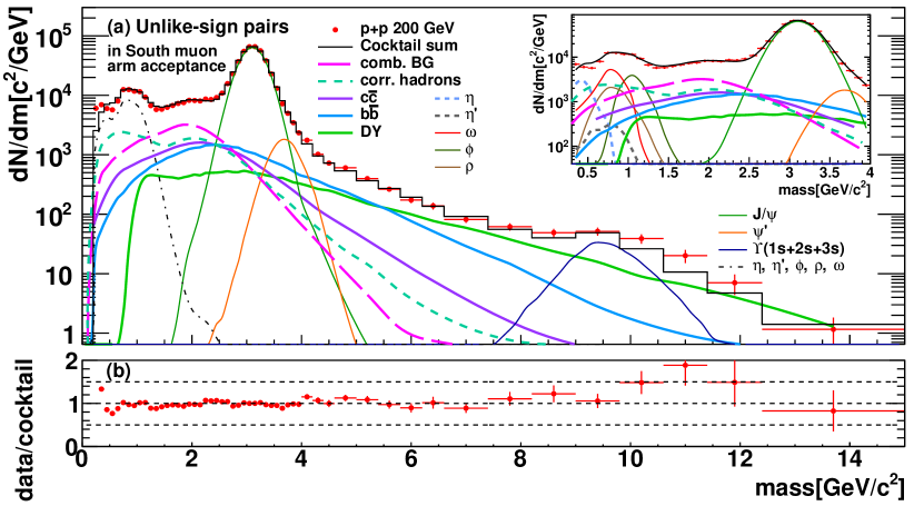
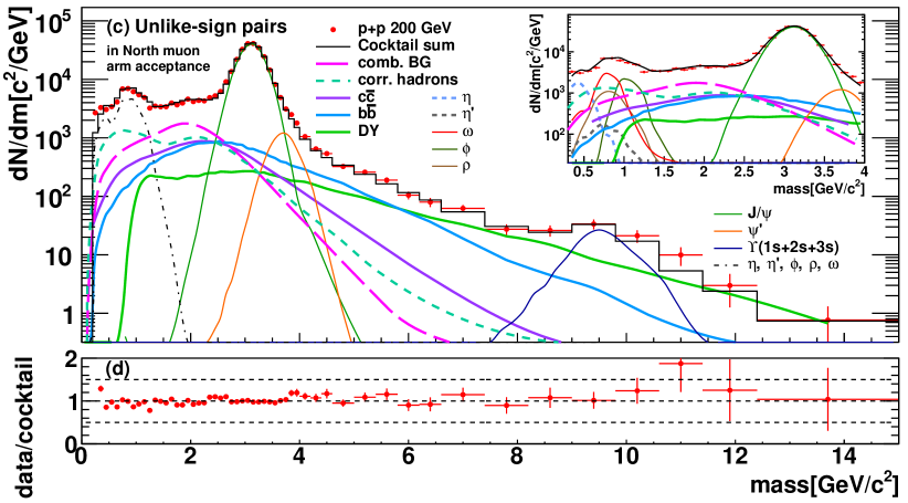
Figure 13: Inclusive $\mu^{+}\mu^{-}$ pair mass distributions from $p$+$p$ collisions at $\sqrt{s}=200$ GeV over the mass range from 0 to 15 GeV/$c^{2}$. The inset shows the mass region below 4 GeV/$c^{2}$ with more detail. Results are shown separately for the (a) south and (c) north muon arms. The data are compared to the cocktail of expected sources. Contributions from $c\bar{c}$ and $b\bar{b}$ are generated using powheg. Panels (b) and (d) show the ratio of the data divided by the known sources.

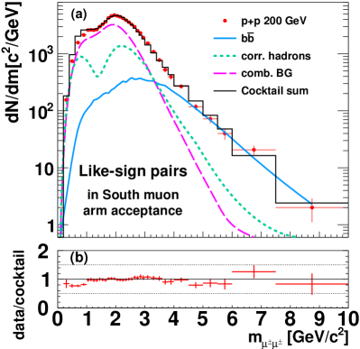
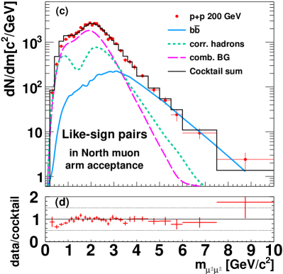
Figure 14: Inclusive like-sign $\mu\mu$ pair yield from $p$+$p$ collisions as a function of mass for the (a) south and (c) north muon arms and (b),(d) the ratio of data to expected sources. Contributions from $b\bar{b}$ are generated using powheg.

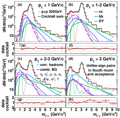
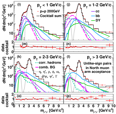
Figure 15: Inclusive unlike-sign $\mu\mu$ pair yield from $p$+$p$ collisions at $\sqrt{s}=200$ GeV as a function of mass in different $p_{T}$ slices for the (a,b,c,d) south and (i,j,k,l) north muon arms. The ratio of data to expected sources are shown in panels (e,f,g,h) for the south arm and (m,n,o,p) for the north arm.

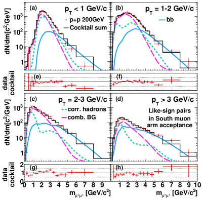
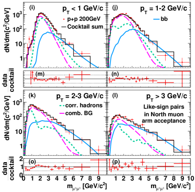
Figure 16: Inclusive like-sign $\mu\mu$ pair yield from $p$+$p$ collisions at $\sqrt{s}=200$ GeV as a function of mass for the (a,b,c,d) south and north (i,j,k,l) muon arms. The ratio of data to expected sources are shown in panels (e,f,g,h) for the south arm and (m,n,o,p) for the north arm.

VI.3 Signal extraction

Different cocktail components contribute with different strength to the muon pair continuum in different mass regions for $\mu^{+}\mu^{-}$ and $\mu^{\pm}\mu^{\pm}$ charge combinations. To obtain differential measurements we identify mass regions for the $c\bar{c}$, $b\bar{b}$, and Drell-Yan signal, where the ratio of the signal to all other $\mu\mu$ pairs is the most favorable for that signal. These regions are referred to in the following as charm, bottom, or Drell-Yan mass region, respectively. The mass regions are:

• Charm: $1.5<m_{\mu^{+}\mu^{-}}<2.5$ GeV/$c^{2}$

• Bottom: $3.5<m_{\mu^{\pm}\mu^{\pm}}<10.0$ GeV/$c^{2}$

• Drell-Yan:

  $4.8<m_{\mu^{+}\mu^{-}}<8.2$ GeV/$c^{2}$

  and $11.2<m_{\mu^{+}\mu^{-}}<15.0$ GeV/$c^{2}$

For each region we extract differential distributions by subtracting all other $\mu\mu$ pair sources.

VI.3.1 Azimuthal correlations and pair $p_{T}$ of $\mu^{+}\mu^{-}$ from $c\bar{c}$

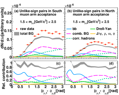
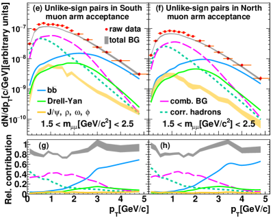
Figure 17: The $\mu\mu$ pair data in the charm mass region as a function of (a,b) $\Delta\phi$ or (c,d) pair $p_{T}$ are shown. Contributions from all known sources other than charm decays are also shown. Panels (c,d,g,h) give the ratio of different components to the total yield. Gray bands indicate the systematic uncertainty on the sum of all contributions.

Figure 17 shows the number of pairs per event as a function of their azimuthal opening angle, $\Delta\phi$, or their pair transverse momentum $p_{T}$ in the charm mass region. The data are compared to all other sources that contribute in this region. For each $\Delta\phi$ or $p_{T}$ bin, the number of pairs from charm decays ($N^{+-}_{c\bar{c}}$) is obtained as:

$$\begin{split}N^{+-}_{c\bar{c}}=N_{\rm incl}^{+-}-N_{b\bar{b}}^{+-}-N_{\rm DY}^{+-}-N_{\rho,\phi,\omega}^{+-}-N_{J/\psi}^{+-}\\ -N_{\rm cor}^{+-}-N_{\rm comb}^{+-},\end{split}$$ (13)

where $N_{\rm incl}^{+-}$ is the number of pairs passing all single and pair cuts in Tables 1 and 2, $N_{b\bar{b}}^{+-}$ is the estimated number of pairs from bottom decays, $N_{\rm DY}^{+-}$ is the estimated number of pairs from Drell-Yan, $N_{\rho,\phi,\omega}^{+-}$ is the estimated number of pairs from low mass vector meson decays, $N_{J/\psi}^{+-}$ is the estimated number of pairs from $J/\psi$ decays, $N_{\rm cor}^{+-}$ is the estimated number of pairs from correlated hadrons, and $N_{\rm comb}^{+-}$ is the estimated number of combinatorial pairs.

VI.3.2 Azimuthal correlations and pair $p_{T}$ of $\mu^{\pm}\mu^{\pm}$ from $b\bar{b}$

The azimuthal opening angle distribution and pair $p_{T}$ distribution for $\mu^{\pm}\mu^{\pm}$ pairs from the bottom mass region is shown in Fig. 18. Besides the $b\bar{b}$ contribution there are also contributions from correlated and combinatorial hadronic pairs. The number of pairs from bottom decays ($N_{b\bar{b}}^{\pm\pm}$) is obtained according to the following relation:

$$N_{b\bar{b}}^{\pm\pm}=N_{\rm incl}^{\pm\pm}-N_{\rm cor}^{\pm\pm}-N_{\rm comb}^{\pm\pm},$$ (14)

where $N_{\rm incl}^{\pm\pm}$ is the number of pairs passing all single and pair cuts in Tables 1 and 2, $N_{\rm cor}^{\pm\pm}$ is the estimated number of pairs from correlated hadrons, and $N_{\rm comb}^{\pm\pm}$ is the estimated number of combinatorial pairs. We subtract the background as a function of $\Delta\phi$ or pair $p_{T}$.

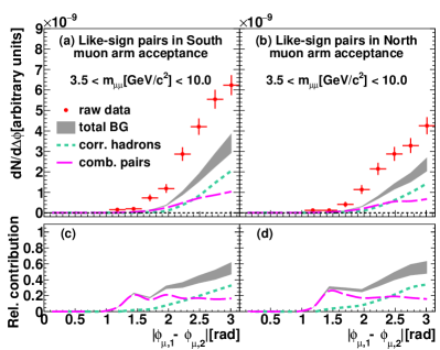
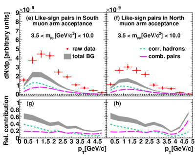
Figure 18: The like-sign $\mu\mu$ pair data in the bottom mass region as a function of (a,b) $\Delta\phi$ or (c,d) pair $p_{T}$ are shown. Contributions from all known sources other than bottom decays are also shown. Panels (c,d,g,h) give the ratio of different components to the total yield. Gray bands indicate the systematic uncertainty on the sum of all contributions.

VI.3.3 Pair mass and $p_{T}$ distribution of $\mu^{+}\mu^{-}$ pairs from Drell-Yan

The Drell-Yan yield is extracted in a mass region that excludes the $\Upsilon$ mass region. The primary sources of background pairs are from bottom and charm decays. The number of pairs from Drell-Yan ($N^{+-}_{\rm DY}$) is obtained as:

$$\begin{split}N^{+-}_{\rm DY}=N_{\rm incl}^{+-}-N_{b\bar{b}}^{+-}-N_{c\bar{c}}^{+-}-N_{J/\psi,\psi^{\prime}}^{+-}\\ -N_{\Upsilon}^{+-}-N_{\rm cor}^{+-}-N_{\rm comb}^{+-},\end{split}$$ (15)

where $N_{\rm incl}^{+-}$ is the number of pairs passing all single and pair cuts in Tables 1 and 2, $N_{J/\psi,\psi^{\prime}}^{+-}$ is the estimated number of pairs from $J/\psi$ and $\psi^{\prime}$ decays, $N_{\Upsilon}^{+-}$ is the estimated number of pairs from the $\Upsilon$ family, $N_{\rm cor}^{+-}$ is the estimated number of pairs from correlated hadrons, and $N_{\rm comb}^{+-}$ is the estimated number of combinatorial pairs. The background contributions as a function of pair mass or $p_{T}$ are shown in Fig. 19.

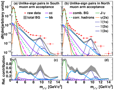
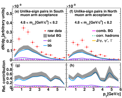
Figure 19: The unlike-sign $\mu\mu$ pair data used to determine the Drell-Yan contribution as a function of (a,b) mass or (c,d) pair $p_{T}$ are shown. Contributions from all known sources other than the Drell-Yan process are also shown. Panels (c,d,g,h) give the ratio of different components to the total yield. Gray bands indicate the systematic uncertainty on the sum of all contributions.

VI.4 Acceptance and Efficiency Corrections

To obtain a physical yield or cross section $\Gamma$, the raw yield $\Gamma_{raw}$ determined in the previous section, must be corrected for detector effects in multiple steps.

$$\begin{split}\Gamma=\Gamma_{raw}\cdot\frac{\sigma_{\rm BBC}}{N_{\rm BBC}\cdot\epsilon_{\rm bias}}\cdot\frac{\alpha}{A\times\epsilon_{\rm rec}},\end{split}$$ (16)

where $\Gamma$ and $\Gamma_{raw}$ can represent differential or integrated quantities. The raw yield is converted to yield per event by dividing by $N_{\rm BBC}$, the number of sampled MB events. The $p$+$p$ cross section sampled by the BBC is $\sigma_{\rm BBC}=23.0\pm 2.2$ mb at $\sqrt{s}=200$ GeV Drees et al. (2003), it relates to the inelastic $p$+$p$ cross section $\sigma_{pp}$:

$$\sigma_{pp}=\frac{\sigma_{\rm BBC}}{\epsilon_{\rm BBC}},$$ (17)

where $\epsilon_{\rm BBC}=0.55\pm 0.06$ is the fraction of inelastic $p$+$p$ collisions recorded by the BBC. The BBC trigger bias for hard scattering events is ${\epsilon_{\rm bias}}=0.79\pm 0.02$ Adler et al. (2007b).

The other factors in Eq. 16 are $\epsilon_{\rm rec}$, the pair reconstruction efficiency that accounts for efficiency losses due to track reconstruction, single track and pair cuts, the software trigger efficiency, and detector inefficiency; $A$, the detector acceptance; and $\alpha$, an additional normalization constant that accounts for effects not included in the Monte-Carlo simulation, which will be described in detail in Sec. VII.4.

The acceptance $A$ has different meanings for the different measurements presented here. The azimuthal opening angle distributions for $\mu\mu$ pairs from $c\bar{c}$ and $b\bar{b}$ are corrected up to the ideal muon arm acceptance, which requires that each muon has a momentum $p>3$ GeV/$c$ and falls in the pseudorapidity range $1.2<|\eta|<2.2$. For the $\mu\mu$ pairs from Drell-Yan production the correction is for the muon pair to be in the rapidity range $1.2<|y^{\mu\mu}|<2.2$. To determine the $b\bar{b}$ cross section we correct up to 4$\pi$, the full phase space as shown in Tab. 3. In general, $A\times\epsilon_{\rm rec}$ is calculated using the default simulation framework. Input from the appropriate physics event generator is run through the simulation; the ratio of the reconstructed $\Gamma_{raw}^{MC}$ yield over the input yield $\Gamma^{MC}$ gives $A\times\epsilon_{\rm rec}$.

Finally, the factor $\alpha$ accounts for the combined effect of double interactions, $\alpha_{double}$; modifications of the reconstruction efficiency due to detector occupancy, $\alpha_{\rm occ}$; the change of the trigger livetime with luminosity, $\alpha_{live}$; and additional variations with luminosity, $\alpha_{lum}$; which are not included in the Monte-Carlo simulations. We determine $\alpha$ by comparing the measured $J/\psi$ cross section Adare et al. (2012) with the result using Eq. 16 with $\alpha=1$. $\alpha=1.38$ for south and north muon arm, respectively. We obtain $\alpha=1.30\pm 0.16$ and $\alpha=1.38\pm 0.17$ for south and north muon arm, respectively. Our values are consistent with the product of the individual factors $\alpha_{double}\times\alpha_{\rm occ}\times\alpha_{live}\times\alpha_{lum}$ within the systematic uncertainties, where the individual factors are determined with data driven methods (see Sec. VII.4).

VI.4.1 Azimuthal correlations and pair $p_{T}$ of $\mu\mu$ from $c\bar{c}$ and $b\bar{b}$

The fully corrected per event pair yield is given by Eq. 18.

$$\begin{split}\frac{dN}{dX}=\frac{N_{\rm HF}}{\Delta X}\cdot\frac{\epsilon_{\rm BBC}}{N_{\rm BBC}\cdot\epsilon_{\rm bias}}\cdot\frac{\alpha}{\epsilon_{\rm rec}(X)},\end{split}$$ (18)

where $X$ is either $\Delta\phi$ or pair $p_{T}$, $\Delta X$ is the corresponding bin width, and $N_{\rm HF}$ refers to $N_{c\bar{c}}^{+-}$ or $N_{b\bar{b}}^{\pm\pm}$ given by Eq. 13 and Eq. 14, respectively. All other factors are the same as in Eq. 16.

The pair reconstruction efficiency $\epsilon_{\rm rec}(X)$ is determined using input distributions from pythia and powheg and is computed by taking the ratio of reconstructed and generated yields with both generated tracks satisfying the condition of the ideal muon arm acceptance ($p>3$ GeV/$c$ and $1.2<|\eta|<2.2$). Here we correct the data up to the ideal muon arm acceptance. We do not correct up to $\mu\mu$ pairs in $1.2<|y_{\mu\mu}|<2.2$ to avoid systematic effects from model dependent extrapolations. Systematic uncertainties for model dependent efficiency corrections are determined by comparing $\epsilon_{\rm rec}(X)$ using pythia or powheg as input distributions. This will be discussed in detail in Section VII.

VI.4.2 Drell-Yan

The differential cross section as a function of mass or $p_{T}$ is given by Eq. 19 and Eq. VI.4.2.

$$\begin{split}\frac{d^{2}\sigma}{dmdy}=\frac{N_{\rm DY}}{\Delta m\Delta y}\cdot\frac{\sigma_{\rm BBC}}{N_{\rm BBC}\cdot\epsilon_{\rm bias}}\cdot\frac{\alpha\cdot\beta(m,y)}{A\times\epsilon_{\rm rec}(m,y)},\end{split}$$ (19)

$$\frac{1}{2\pi p_{T}} \frac{d^{2}\sigma}{dydp_{T}}=$$

$$\frac{N_{\rm DY}}{2\pi p_{T}\Delta y\Delta p_{T}}\cdot\frac{\sigma_{\rm BBC}}{N_{\rm BBC}\cdot\epsilon_{\rm bias}}\cdot\frac{\alpha\cdot\beta(y,p_{T})}{A\times\epsilon_{\rm rec}(y,p_{T})},$$ (20)

where $N_{\rm DY}$ is raw yield of pairs from Drell-Yan given by Eq. 15. $\Delta m$, $\Delta p_{T}$, and $\Delta y$ are the bin widths in pair mass, pair $p_{T}$ and pair rapidity respectively. The factors $\beta(m,y)$ and $\beta(y,p_{T})$ correct the cross section averaged over the bin to the cross section at the bin center. These correction factors are estimated using pythia simulations and lie between 0.97 and 1.03. All other factors are the same as in Eq. 16.

The pair acceptance and efficiency $A\times\epsilon_{\rm rec}(m,y)$ and $A\times\epsilon_{\rm rec}(y,p_{T})$ are determined using input distributions generated using pythia. It corrects the pair yield to one unit of rapidity at $1.2<|y^{\mu\mu}|<2.2$.

VI.4.3 Bottom cross section

We also determine the $b\bar{b}$ cross section from the measured $\mu\mu$ pair yield from $b\bar{b}$. In the fitting procedure we determined the normalization $\kappa_{b\bar{b}}$, which was chosen such that it directly relates to the $\sigma_{b\bar{b}}$ cross section:

$$\sigma_{b\bar{b}}=\frac{\alpha\cdot\sigma_{\rm BBC}}{N_{\rm BBC}\cdot\epsilon_{\rm bias}}\cdot\kappa_{b\bar{b}}.$$ (21)

The acceptance and efficiency corrections, trigger efficiency, branching ratios, and oscillation parameters are all implicitly encapsulated in $\kappa_{b\bar{b}}$, because the templates for fitting already include all the aforementioned considerations.

We used two models pythia and powheg, to take into account a possible model dependence. The extrapolation from the limited phase space of our $\mu\mu$ measurement to the entire kinematic region can be divided into four steps:

• Extrapolation from $\mu^{\pm}\mu^{\pm}$ muon pairs with $m_{\mu\mu}>3$ GeV/$c^{2}$ in the ideal muon arm acceptance to all muon pairs ($\mu^{\pm}\mu^{\pm}$ and $\mu^{+}\mu^{-}$) with $m_{\mu\mu}>3$ GeV/$c^{2}$ in the ideal muon arm acceptance.

• Extrapolation to all muon pairs in the entire mass region ($m_{\mbox{$\mu\mu$}}>0$ GeV/$c^{2}$) in the ideal muon arm acceptance.

• Extrapolation to all muon pairs with the pseudorapidity of each muon satisfying $1.2<|\eta_{\mu}|<2.2$.

• Extrapolation to muon pairs in $4\pi$.

Table 3: Step by step reduction of phase space for $\mu\mu$ pairs from $b\bar{b}$ production; starting from all $\mu\mu$ pairs produced to like-sign $\mu\mu$ pairs with $m_{\mu\mu}>3$ GeV/$c^{2}$ in the ideal muon arm acceptance. All numbers represent the number of $\mu\mu$ pairs per generated pythia or powheg $b\bar{b}$ event in the specified phase space. Each step is cumulative to the previous, i.e. each row includes one more restriction to the $\mu\mu$ phase space. The factors in brackets quantify the decrease of the number of pairs from the previous step.

	Event gen.
condition	pythia	powheg
$4\pi$	$6.76\times 10^{-2}~{}(15.4)$	$6.73\times 10^{-2}~{}(15.6)$
$1.2<|\eta_{\mu}|<2.2$	$4.39\times 10^{-3}~{}(10.7)$	$4.32\times 10^{-3}~{}(10.7)$
$p_{\mu}>3$ GeV/$c$	$4.11\times 10^{-4}~{}(3.48)$	$4.04\times 10^{-4}~{}(3.39)$
$m_{\mu\mu}>3$ GeV/$c^{2}$	$1.18\times 10^{-4}~{}(3.19)$	$1.19\times 10^{-4}~{}(3.48)$
$\mu^{\pm}\mu^{\pm}$ in PHENIX	$3.71\times 10^{-5}$	$3.42\times 10^{-5}$

Table 3 quantifies each step. For clarity they are shown in reversed order. One can see that in each step, the difference between pythia and powheg is less than $8\%$, which is consistent with the observation from Ref. Adare et al. (2015), that the model dependence of the extrapolation is small because the $\mu\mu$ (or $ee$) pair distributions from bottom are dominated by decay kinematics.

The differential cross section $d\sigma_{b\bar{b}}/dy_{b}|_{\langle y_{b}\rangle=\pm 1.7}$ can be calculated as follows:

$$\frac{d\sigma_{b\bar{b}}}{dy_{b}}|_{\langle y_{b}\rangle=\pm 1.7}=\frac{\alpha\cdot\sigma_{\rm BBC}}{N_{\rm BBC}\cdot\epsilon_{\rm bias}}\cdot\frac{dN_{b}}{dy_{b}}|_{\langle y_{b}\rangle=\pm 1.7}\cdot\kappa_{b\bar{b},\frac{N}{S}},$$ (22)

where $dN_{b}/dy_{b}|_{\langle y_{b}\rangle=\pm 1.7}$ is the rapidity density of $b$ quarks determined from the average of pythia and powheg, $\kappa_{b\bar{b},\frac{N}{S}}$ is the fitted normalization for bottom from the north (south) muon arm.

VII Systematic uncertainties

We consider four types of sources of possible systematic uncertainties on the extraction of $\mu\mu$ pairs from $c\bar{c}$, $b\bar{b}$, and Drell-Yan. These are uncertainties:

• on the shape of the template distributions,

• on the normalization of template distributions,

• on the acceptance and efficiency corrections,

• and on the overall global normalization.

The first three sources of systematic uncertainties are point-to-point correlated, but allow for a gradual overall change in the shape of the distributions. We refer to these uncertainties as type B. Global normalization uncertainties do not affect the shape of the distributions but only the absolute normalization; these are quoted separately as type C.

There are multiple contributors to each type of systematic error, for example the $c\bar{c}$ and $b\bar{b}$ templates are model dependent and can be determined with pythia or powheg. For each such case we repeat the full analysis with the various assumptions. The spread of the results around the default analysis is used to assign systematic uncertainties.

If we considered two assumptions, like in the example given, we quote the uncertainty as half the difference between the two assumptions. If there is a clearly preferred default case, we use the difference of results obtained with extreme assumptions to assign systematic uncertainties.

We quantify all systematic uncertainties as standard deviations. The systematic uncertainties on the different measurements are summarized in Table. 4. For the differential distributions of $c\bar{c}$, $b\bar{b}$, and Drell-Yan, the systematic uncertainties vary with azimuthal opening angle, pair $p_{T}$ or mass as shown in Fig. 20.

Table 4: Summary of arm-averaged relative systematic uncertainties for the total bottom cross section $\sigma_{b\bar{b}}$, the differential Drell-Yan cross section $d^{2}\sigma_{DY\rightarrow\mu\mu}/dmdy$, and the $b\bar{b}$ ($c\bar{c}$) differential yields $dN_{b\bar{b}(c\bar{c})\rightarrow\mu\mu}/d\Delta\phi$. The systematic uncertainty type is indicated in the second column and is applicable only to the differential measurements. The uncertainties for the differential measurements vary with azimuthal opening angle, pair $p_{T}$, or mass. Asymmetric uncertainties are quoted in bracketed values. For the $c\bar{c}$ measurement, the regions $\Delta\phi<\pi/2$, $p_{T}<0.5$ GeV/$c$ and $p_{T}>2.0$ GeV/$c$ are excluded because the yield approaches zero and relative systematic uncertainties diverge. With these regions excluded, the difference between the systematic uncertainties of all measurements for the south and north muon arms differs by no greater than $2\%$ for all systematic uncertainties sources.

	type	$\sigma_{b\bar{b}}$	$\frac{dN_{b\bar{b}\rightarrow\mu\mu}}{d\Delta\phi}$	$\frac{dN_{b\bar{b}\rightarrow\mu\mu}}{dp_{T}}$	$\frac{d^{2}\sigma_{DY\rightarrow\mu\mu}}{dmdy}$	$\frac{1}{2\pi p_{T}}\frac{d^{2}\sigma_{DY\rightarrow\mu\mu}}{dyp_{T}}$	$\frac{dN_{c\bar{c}\rightarrow\mu\mu}}{d\Delta\phi}$	$\frac{dN_{c\bar{c}\rightarrow\mu\mu}}{dp_{T}}$
Input hadron spectra	B	$+$4.7%	$+$($<$6%)	$+$($<$12%)	$+$($<$14%)	$+$($<$20%)	$+$($<$9%)	$+$($<$9%)
		$-$11.0%	$-$($<$19%)	$-$($<$25%)	$-$($<$7%)	$-$($<$9%)	$-$($<$4%)	$-$($<$4%)
Hadron simulation	B	2%	$<$1%	$<$1%	$<$1%	$<$1%	$<$1%	$<$1%
$c\bar{c}$ (shape)	B	2%	$<$4%	$<$5%	$<$4%	$<$6%	-	-
$b\bar{b}$ (shape)	B	-	-	-	$<$14%	$<$17%	$<$3%	$<$3%
Drell-Yan (shape)	B	$<$1%	$<1$%	$<$1%	-	-	$<$6%	$<$5%
ZYAM normalization	B	$<$1%	$<$1%	$<$1%	$<$1%	$<$1%	$<$2%	$<$3%
pythia $h$-$h$ correlations	B	-	-	-	-	-	$<$14%	$<$13%
Simulations($\phi$,$z$)	B	$<$1%	$<4$%	$<5$%	$<$1%	$<$1%	$<8$%	$<$8%
Fitting range	B	$2$%	$<$1%	$<$1%	$<1$%	$<1$%	$<$1%	$<$1%
$\phi,\omega,\rho,J/\psi,\psi^{\prime},\Upsilon$ norm.	B	-	-	-	$<$2%	$<1$%	$<$1%	$<$1%
Statistical uncertainty in fit	B	-	$<$4%	$<$4%	$<$6%	$<$8%	$<$10%	$<$10%
$b\bar{b}$ model dep. extrapolation	-	6.5%	-	-	-	-	-	-
Model dep. eff. corrections	B		$<$10%	$<$3%	-	-	$<$5%	$<$4%
Trigger efficiency	B	1.5%	1.5%	1.5%	1.5%	1.5%	1.5%	1.5%
MuTr efficiency	B	4%	4%	4%	4%	4%	4%	4%
MuID efficiency	B	2%	2%	2%	2%	2%	2%	2%
Sum of type B	-	$+$9.3%	$+$(4%–11%)	$+$(6%–14%)	$+$(4%–21%)	$+$(13%–28%)	$+$(10%–28%)	$+$(10%–20%)
systematic uncertainties		$-$13.2%	$-$(4%–22%)	$-$(6%–26%)	$-$(4%–17%)	$-$(11%–22%)	$-$(10%–20%)	$-$(8%–16%)
Global normalization	C	12%	12%	12%	12%	12%	12%	12%

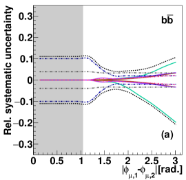
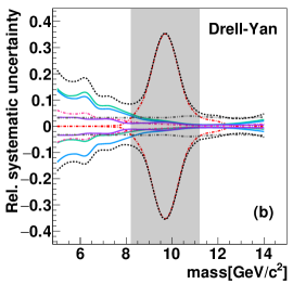
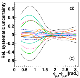
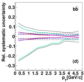
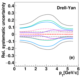
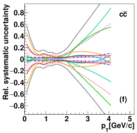
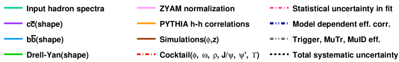
Figure 20: Relative two-arm averaged systematic uncertainties for $c\bar{c}$ and $b\bar{b}$ measurements as a function of $\Delta\phi$ or pair $p_{T}$ and Drell-Yan measurement as a function of mass or $p_{T}$. The shaded regions are excluded from the respective measurements.

VII.1 Shape of simulated distributions

The $c\bar{c}$, $b\bar{b}$, Drell-Yan, and hadronic pair background components are correlated through the fitting procedure, thus an uncertainty on the shape for any one template distribution will affect the fit results of all four components simultaneously. For example, if one increases the hardness of the input pion $p_{T}$ spectrum, the number of high mass like-sign hadron-hadron pairs will increase, which will lead to a smaller $\mu^{\pm}\mu^{\pm}$ pair yield from $b\bar{b}$. Because $b\bar{b}$ is the main competing source to the Drell-Yan process in the high $\mu^{+}\mu^{-}$ pair mass region, this will in turn lead to a larger Drell-Yan yield. Drell-Yan and bottom both contributes to the intermediate mass region where $c\bar{c}$ is extracted, and hence will also modify the $c\bar{c}$ yield.

In the following we will discuss the uncertainties on the shape of individual contributions and how these uncertainties propagate to the measurement of all components.

VII.1.1 Input hadron spectra

The input pion and kaon $p_{T}$ spectra are tuned to match PHENIX and BRAHMS data at $\langle y\rangle=0$ and $\langle y\rangle=2.95$, respectively. This is achieved by applying weighting factors ($w_{h}(y)$) to the $p_{T}$ spectra from pythia, which are determined by a linear interpolation between the two ratios of pythia to the data at $\langle y\rangle=0$ and $\langle y\rangle=2.95$ (see Fig. 9). To estimate the systematic uncertainties on the input hadron $p_{T}$ spectra, we vary the weighting function. We use either $w_{h}(\langle y\rangle=0)$ for all light hadrons, which gives a harder $p_{T}$ spectra than the default case, or $w_{h}(\langle y\rangle=2.95)$, which gives a softer $p_{T}$ spectra. The shape of the hadron-hadron pair mass distribution changes significantly only for masses above 3 GeV/$c^{2}$.

We take the difference of the cross sections obtained using these two sets of $p_{T}$ spectra and the default $p_{T}$ spectra as a systematic uncertainty on the input hadron spectra. For $\sigma_{b\bar{b}}$, this is determined to be ${+4.7\%}$ and ${-11.0\%}$. The uncertainties are also propagated to the $b\bar{b}$ and $c\bar{c}$ azimuthal opening angle distributions and the Drell-Yan yields. In all cases this is a dominant contributor to the systematic uncertainties (see Table 4).

We have also considered using the bands shown in Fig. 9 as limits for the weighting factors, which lead to smaller uncertainties and we choose to quote the more conservative estimate. Uncertainties related to the choice of parton distribution function (PDF) are estimated by evaluating the differences obtained with simulations using the CTEQ5, CTEQ6, MRST2001(NLO) Martin et al. (2002) and GRV98(LO) Glück et al. (1998) parton distribution functions. The differences are negligible compared to the uncertainty due to shapes of the light hadron $p_{T}$ spectra.

VII.1.2 Hadron simulation

The default PHENIX geant4 simulation utilizes the standard HEP physics list QGSP-BERT. For hadronic interactions of pions, kaons and nuclei above 12 GeV, the quark gluon string model (QGS) is applied for the primary string formation and fragmentation. At lower energies, the Bertini cascade model (BERT) is used, which generates the final state from an intranuclear cascade.

To estimate possible uncertainty due to the description of the hadronic interactions in the absorbers, we have used two other physics lists: The (i) FTFP-BERT list, which replaces QGS with the Fritiof model (FTF) for high energies. The FTF uses an alternative string formation model followed by the Lund fragmentation model. And (ii) QGSP-BIC where the low energy approach is replaced by the binary cascade model (BIC), which was optimized to describe proton and neutron interactions, but is less accurate for pions.

Using these different physics lists leads to a 2% difference of $\sigma_{b\bar{b}}$, and a negligible difference to the charm and Drell-Yan normalizations.

VII.1.3 Charm and bottom simulation

There are potential model dependencies of the $\mu\mu$ and muon-hadron templates for $c\bar{c}$ and $b\bar{b}$. To estimate these we compare the $\mu\mu$ and muon-hadron templates obtained using pythia and powheg. Systematic uncertainties on charm and bottom are assumed to be uncorrelated and are added in quadrature.

Due to the large mass of the bottom quark, decay kinematics govern the shape of the distributions, hence the difference between pythia and powheg is small (see Fig. 8). The largest effect of this uncertainty is exhibited at mass $\sim 5$ GeV/$c^{2}$ for the Drell-Yan measurement where the contribution of $b\bar{b}$ is around 40% of the total yield.

For charm, the model dependence is larger than that of bottom, particularly for $m<1$ GeV/$c^{2}$. In the high mass region powheg tends to predict higher yields for both $\mu\mu$ and muon-hadron templates, which is likely due to a harder single muon $p_{T}$ spectrum. However, this has a small effect on the extraction of bottom and Drell-Yan yields in the high mass region where the contribution of charm is less than 10%.

VII.1.4 Drell-Yan

The intrinsic $k_{T}=1.1$ GeV/$c$ used in the pythia simulations is determined by minimizing $\chi^{2}$ of the $p_{T}$ distribution of Drell-Yan pairs in the Drell-Yan mass region, between data and simulations. Background components (mostly from $c\bar{c}$ and $b\bar{b}$) are normalized using cross sections obtained from the procedure and subtracted as a function of $p_{T}$. We find that an intrinsic $k_{T}$ of 1.1 GeV/$c$ best describes the $p_{T}$ distribution of Drell-Yan pairs in the high mass region (see Fig. 21).

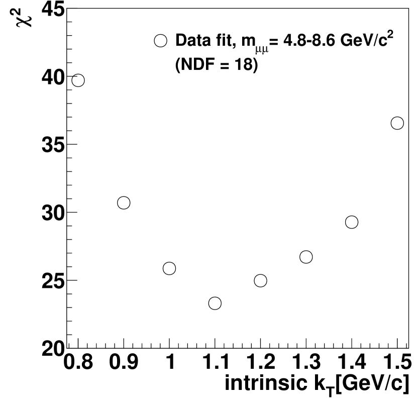
Figure 21: The $\chi^{2}$ for the pair $p_{T}$ spectrum of Drell-Yan pairs in the mass region 4.8–8.6 GeV/$c^{2}$ compared to pythia simulations with different intrinsic $k_{T}$. The $\chi^{2}$ is minimized at a $k_{T}$ of 1.1 GeV/$c$.

We vary the $k_{T}$ by $\pm 0.1$ GeV/$c$ where the $\chi^{2}$ changes by $\sim 1$ to estimate uncertainties in the Drell-Yan distributions. The uncertainty mainly affects the $c\bar{c}$ yield at $\Delta\phi<\pi/2$ and $p_{T}>2$ GeV/$c$ and is negligible elsewhere.

VII.1.5 ZYAM normalization

To estimate the effect of varying the relative contributions between correlated and uncorrelated pairs, we have varied the mass region which we use for the $\Delta\phi_{prim}$ distribution. Instead of the default normalization region $\mathcal{M}$ below 3 GeV/$c^{2}$, we picked 3 separate regions: 0.7–1.3 GeV/$c^{2}$, 1.3–1.6 GeV/$c^{2}$, 1.6–2.2 GeV/$c^{2}$. This results in a variation of the ratio of correlated to uncorrelated pairs by $\pm$10%. The relative effect on the sum of correlated and uncorrelated pairs is less than 2% over the entire mass region, and has a negligible effect on the determination of $b\bar{b}$, $c\bar{c}$, and Drell-Yan cross sections.

VII.1.6 Hadron-hadron correlations from pythia

For the measurement of $c\bar{c}$ yields as a function of $\Delta\phi$ or pair $p_{T}$, correlated hadron pairs are a major background source. To estimate the uncertainty in the description of Tune A pythia, we compare distributions of like-sign pairs between data and simulation in the same mass region (1.5–2.5 GeV/$c^{2}$) where other contributions, including $b\bar{b}$ are negligible. We observe that the width of the back-to-back peak at $\Delta\phi=\pi$ is slightly wider in data compared to pythia simulation. This is seen in the $p_{T}$ distributions as well, because $p_{T}$ is strongly correlated with $\Delta\phi$. The discrepancy is strictly less than 12% and varies with $\Delta\phi$ or $p_{T}$. One data driven approach would be to apply an additional weight to the unlike-sign hadronic pair background as a function of $\Delta\phi$ or $p_{T}$, where the weight is computed by taking the ratio between data and simulations using the like-sign pairs as a function of $\Delta\phi$ or $p_{T}$ in the same mass region. This is motivated by the fact that the like-sign pairs are dominated by hadronic contributions in the mass region of interest.

Here we take the average between the Tune A setup and this data driven modification to be our central value, and assign a systematic uncertainty on the $c\bar{c}$ yields as the difference between these two approaches. The resultant systematic uncertainty is strongly $\Delta\phi$ and $p_{T}$ dependent, ranging from $0\%$ to $14\%$.

VII.1.7 Azimuthal angle($\phi$) description in simulations

We compare the $\phi$ distributions of single tracks in data, simulations with the default framework, and the FastMC. We find reasonable agreement between data and the default simulation and conclude that the uncertainty from the default simulation framework is negligible. However, for simulations using the FastMC, we approximated the relative $\phi$ dependent efficiency by a weighting strategy in $\phi$ bins of finite width, which gives rise to a small smearing in the $\phi$ (and hence $\Delta\phi$ and to a lesser extent $p_{T}$) distributions (see Fig. 36). We assign $5\%$ uncertainty to the $\Delta\phi$ distributions generated using the FastMC, which is estimated by comparing $\Delta\phi$ distributions of mixed pairs between FastMC and real data. This in turn gives rise to an average of $5\%$ and $3\%$ to the $c\bar{c}$ and $b\bar{b}$ differential yields respectively.

VII.1.8 $z$-vertex description of simulations

We have generated hadronic pairs in discrete $z_{\rm vtx}$ regions that cover 1/4 of the full collision $z_{\rm vtx}$ region using the FastMC. Figure 22 shows a comparison of data and simulations in different $z_{\rm vtx}$ regions after the initial normalization (Sec. VI.1.2) and iterative fitting procedure (Sec. VI.2). We see good agreement between the simulations and data in all $z_{\rm vtx}$ regions; there is no indication that the approximations in the $z_{\rm vtx}$ description of correlated hadrons is biasing the fit of the like-sign pairs.

To estimate the systematic uncertainty on this approximation, recall that the yield of decay muons varies linearly with $z_{\rm vtx}$, whereas the yield of prompt muons is constant Aidala et al. (2017a). Thus, the main effect of the $z_{\rm vtx}$ approximation is the uncertainty on the prompt muon to decay muon ratio. In the FastMC the ratio is determined in three vertex bins of 5 cm width at $z_{\rm vtx}=$ -20, 0, and 20 cm, instead of the full 20 cm $z_{\rm vtx}$ slices. We assign a systematic uncertainty by varying the prompt muon to decay muon ratio separately for each $z_{\rm vtx}$ region. Because prompt muons are dominated by charm decays, we estimate this effect by varying the charm cross section by $\pm 15\%$ for one particular $z$ slice separately. The effect on the fitted $b\bar{b}$ cross section is $\sim 1\%$ and is negligible compared to other sources of systematic uncertainties.

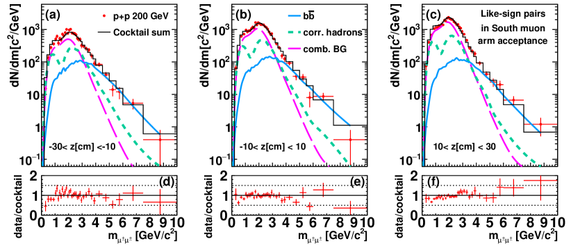
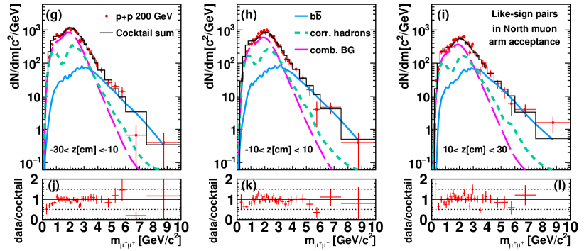
Figure 22: Inclusive like-sign $\mu\mu$ pair yield from $p$+$p$ collisions at $\sqrt{s}=200$ GeV as a function of mass in three $z$ vertex bins for the south and north muon arms. The data are compared to the contributions from $b\bar{b}$ decays, and the correlated & combinatorial contribution from hadronic pairs.

VII.2 Normalization of simulated distributions

In addition to uncertainties due to the shape of distributions, uncertainties on the normalization of one component can affect the yield of other components. We list sources of such uncertainties in this section.

VII.2.1 Fitting

To estimate uncertainties in the fit range, we vary the lower bound of the fit range of like-sign pairs from $m=1.0$ GeV/$c^{2}$ to $m=2.0$ GeV/$c^{2}$. The variation in $\sigma_{b\bar{b}}$ is around $2\%$ and is assigned as the systematic uncertainty on the fit range. The unlike-sign fit range is also varied to diagnose possible effects due to non Gaussian tails of the mass distribution of $\mu^{+}\mu^{-}$ pairs from resonance decays. The variation of $\kappa_{c\bar{c}}$ is less than 5% with different fit ranges in the unlike-sign, and this $\kappa_{c\bar{c}}$ variation propagates into $<1$% variation in $\sigma_{b\bar{b}}$.

We estimate possible uncertainties due to the stability of the fit by varying the binning of distributions. The variations are negligible compared to the statistical uncertainty. We therefore do not assign systematic uncertainties on fit stability.

VII.2.2 Normalization of cocktail components

The vector mesons $\phi,~{}\omega,~{}\rho,~{}J/\psi,~{}\psi^{\prime}$, and $\Upsilon$ are background components to determine $N_{c\bar{c}}^{+-}$ and $N_{\rm DY}^{+-}$ in Eq. 13 and 15, respectively. Their normalizations are fixed using previous measurements. The normalization of each component has associated statistical and systematic uncertainties from those measurements. We add these uncertainties in quadrature and vary normalizations of these background components to estimate propagated uncertainties in $N_{c\bar{c}}^{+-}$ and $N_{\rm DY}^{+-}$. Because the template fit excludes all mass regions dominated by resonance decays, the uncertainty from the normalizations of the resonances only have a minor effect of less than 2% on the fit results, which is negligible compared to other sources of uncertainties.

VII.2.3 Statistical uncertainty in fit result

Charm, bottom, and hadronic pairs are background components for $N_{\rm DY}^{+-}$. The statistical uncertainties on fitted values of $\kappa_{c\bar{c}}$, $\kappa_{b\bar{b}}$, and $\kappa_{h}$ become a source of systematic uncertainty for $N_{\rm DY}^{+-}$. Similarly, systematic uncertainties for $N^{+-}_{c\bar{c}}$ arise from statistical uncertainties on $\kappa_{h}$, $\kappa_{\rm DY}$, and $\kappa_{b\bar{b}}$, and $N_{b\bar{b}}^{\pm\pm}$ from $\kappa_{h}$ and $\kappa_{c\bar{c}}$. The statistical uncertainties for $\kappa_{b\bar{b}}$ and $\kappa_{\rm DY}$ is $\sim 8\%$, and for $\kappa_{h}$ is $\sim 2\%$ for each arm. The associated systematic uncertainty depends heavily on the signal to background ratio and varies from measurement to measurement.

VII.3 Extrapolation, acceptance and efficiency

This section details systematic uncertainties related to acceptance and efficiency.

VII.3.1 Model dependence on $b\bar{b}$

We use the high mass like-sign pairs to constrain $\sigma_{b\bar{b}}$, hence a determination of $d\sigma_{b\bar{b}}/dy$ involves an extrapolation to zero mass at forward rapidity, whereas the determination of $\sigma_{b\bar{b}}$ involves a further extrapolation to the full rapidity region. This is dependent on correlations between $\mu\mu$ pairs from bottom as well as the oscillation parameters and branching ratios. To quantify the uncertainty in the extrapolation, we take the average of the fitted cross section $\sigma_{b\bar{b}}$ using pythia and powheg and assign the difference ($\pm 6.5\%$) as the systematic uncertainty. We note that the difference between the default values of the time-integrated probability for a neutral $B^{0}_{d}$ ($B^{0}_{s}$) to oscillate $\chi_{d}$ ($\chi_{s}$) of pythia and the values from the PDG, $\chi_{d}=0.1860\pm 0.0011$ ($\chi_{s}=0.499304\pm 0.000005$) Patrignani et al. (2016) is less than $2\%$ and hence much less than the assigned uncertainty.

VII.3.2 Model dependence on efficiency correction

The charm and bottom azimuthal opening angle distributions are corrected to represent $\mu\mu$ pairs the ideal muon arm acceptance. To assess the sensitivity to different input distributions we compare the efficiency as a function of $\Delta\phi$ calculated using pythia and powheg. No model dependence of the efficiency corrections is observed for $\mu\mu$ pairs with $\Delta\phi>1.5$ from $c\bar{c}$ and $b\bar{b}$. For $\Delta\phi<1.5$, we assign an additional uncertainty based on the difference of the efficiency corrections calculated by pythia and powheg.

The charm and bottom pair $p_{T}$ spectra are also corrected to represent the muon arm acceptance. No model dependence of the efficiency corrections is observed for $\mu\mu$ pairs in the measured $p_{T}$ range. We assign an uncertainty based on the statistical uncertainty of the calculated efficiency corrections.

For Drell-Yan, we estimate the model dependence of the acceptance and efficiency corrections by varying the intrinsic $k_{T}$ settings of pythia within the systematic limits as described in Sec. VII.1.4. No model dependence of the acceptance and efficiency corrections is observed. We assign an uncertainty based on the statistical uncertainty of the calculated efficiency corrections.

VII.3.3 Trigger efficiency

The possible discrepancy between the software trigger emulator and the hardware trigger is quantified by comparing the real data trigger decision with the offline software trigger. We find that they differ by within $1.0\%$ and $1.5\%$ for the south and north arm, respectively. We use these values as estimates of the associated systematic uncertainty.

VII.3.4 Reconstruction efficiency

The muon track reconstruction and muon identification used in this analysis is the standard PHENIX muon reconstruction chain. The systematic uncertainties have been previously studied. We assign MuTr ($4\%$) and MuID ($2\%$) as systematic uncertainties on reconstruction efficiency based on the work published in Aidala et al. (2017a).

VII.4 Global normalization uncertainties

The absolute normalization of the $\mu\mu$ pair spectra is set by the measured $J/\psi$ yield Adare et al. (2012), which is measured with an accuracy of 12%. This is the systematic uncertainty on the scale for all results presented in this paper.

The normalization is expressed in Eq. 16 by the factor $\alpha$, which accounts for the combined effect of the change of the trigger livetime with luminosity $\alpha_{live}$, modifications of the reconstruction efficiency due to detector occupancy $\alpha_{\rm occ}$, additional variations of the efficiencies with luminosity $\alpha_{lum}$, and the effect of double interactions $\alpha_{double}$.

As a cross-check, these individual factors were determined separately. The trigger livetime was monitored during data taking and the correction was found to be 1.35 (1.30) for the south(north) arm, respectively. The occupancy effect was studied by embedding simulated $\mu\mu$ pairs in $p$+$p$ events and results in $\alpha_{\rm occ}=1.06\ (1.04)$. In addition, there is a drop of the detector efficiency with increasing beam intensity that was found to give $\alpha_{lum}=1.04\ (1.07)$.

Finally, the approximately 20% double interactions in the sample increase the pair yield by about 11%, resulting in $\alpha_{double}=0.90$. The yield increase is smaller than the number of double interactions mostly for two reasons. Diffractive events contribute to events with double interactions but do not contribute significantly to the pair yield. Events with double interactions contain collisions more than 40–50 cm away from the nominal collision point; pairs from these events have significantly reduced reconstruction efficiency. The combination of both effects approximately cancel the efficiency losses due to detector occupancy and high interaction rates.

The product of individual corrections to the normalization is $\alpha_{double}\times\alpha_{\rm occ}\times\alpha_{live}\times\alpha_{lum}$ = 1.33 (1.34) for the south (north) arm. These values are consistent within uncertainties with $1.30\pm 0.16$ ($1.38\pm 0.17$), the values based on the $J/\psi$ measurement.

VIII Results

VIII.1 Azimuthal opening angle and pair $p_{T}$ distributions for $\mu\mu$ pairs from $c\bar{c}$ and $b\bar{b}$

The fully corrected $\mu\mu$ pair yield from $c\bar{c}$ and $b\bar{b}$ decays are shown in Figs. 23 and 24 as a function of $\Delta\phi$ and pair $p_{T}$. The muons are in the nominal acceptance of $p>3$ GeV/$c$ and $1.2<|\eta|<2.2$. The pairs are in selected mass ranges of $1.5<m_{\mu^{+}\mu^{-}}<2.5$ GeV/$c^{2}$ and $3.5<m_{\mu^{\pm}\mu^{\pm}}<10.0$ GeV/$c^{2}$ for $c\bar{c}$ and $b\bar{b}$, respectively. The yields for the two pseudorapidity regions are consistent with each other. Due to the mass selection, the $\Delta\phi$ and $p_{T}$ distributions are highly correlated with each other.

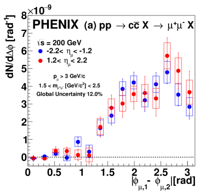
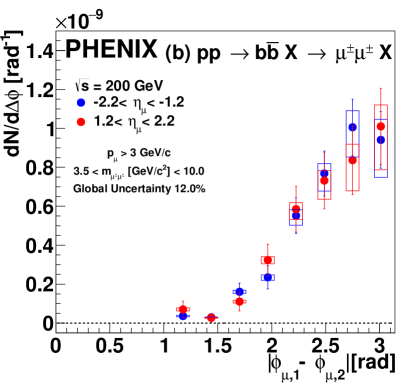
Figure 23: The corrected $\mu\mu$ yield as a function of $\Delta\phi$ from (a) charm and (b) bottom decays. The error bars correspond to statistical uncertainties, and the boxes correspond to the type B systematic uncertainties. The $12.0\%$ type C systematic uncertainty is not shown. Results are given separately for the south and north muon arms.

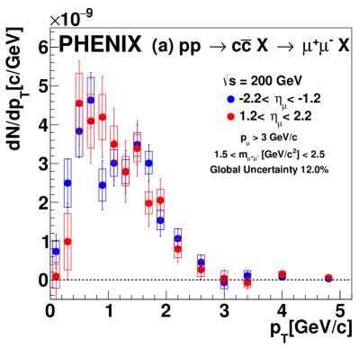
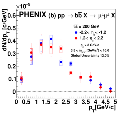
Figure 24: The corrected $\mu\mu$ yield as a function of pair $p_{T}$ from (a) charm and (b) bottom decays. The error bars correspond to statistical uncertainties, and the boxes correspond to the type B systematic uncertainties. The additional $12.0\%$ type C systematic uncertainty is not shown. Results are presented separately for the south and north muon arms.

The spectra for the two pseudorapidity regions are combined using the method documented in Appendix B and compared to model calculations based on pythia and powheg. The comparison is shown in Figs. 25 and 26. Pairs generated by the models are filtered with the same kinematic cuts that are applied in the data analysis. The model curves are normalized using the fitting procedure outlined in Sec. VI.2.

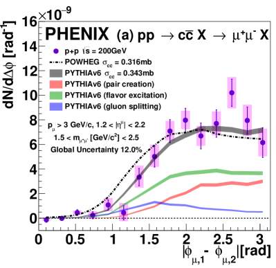
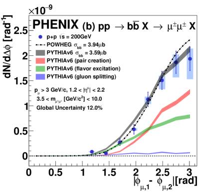
Figure 25: The corrected $\mu\mu$ yield as a function of azimuthal opening angle from (a) charm and (b) bottom decays. The data are compared to the distributions calculated with powheg and pythia. The model calculations are normalized to the data (see text for details). For pythia the $\mu\mu$ pair yield is broken down into contributions from pair creation, flavor excitation, and gluon splitting.

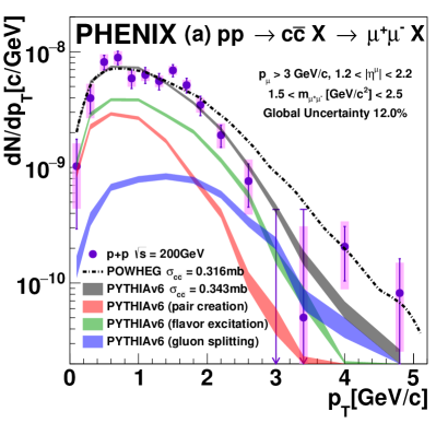
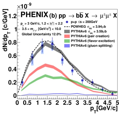
Figure 26: The corrected $\mu\mu$ yield as a function of pair $p_{T}$ from (a) charm and (b) bottom decays. Presentation of the comparison to powheg and pythia is the same as Fig. 25. The upper limits on panel (a) indicate 95% confidence level (For a data point with value $d$ and statistical uncertainty $\sigma$, the upper limit $u$ is determined by the following relation: $\int_{0}^{u}f/\int_{0}^{\infty}f=0.95$, where $f$ is a Gaussian distribution with mean $d$ and width $\sigma$.)

For $c\bar{c}$ the model calculations are normalized in the kinematic region $1.4<m<2.5$ GeV/$c^{2}$ and $p_{T}<2$ GeV/$c$ to the data. Consequently, as seen in Fig. 26, the $p_{T}$ spectrum is adequately described by both pythia and powheg for $p_{T}<2$ GeV/$c$. However, for $p_{T}>2$ GeV/$c$, the yield predicted by powheg is systematically higher than the data, while the yield from pythia is more consistent with the data.

The larger yield predicted by powheg also manifests itself in the $\Delta\phi$ projection at $\Delta\phi<1.5$. For $c\bar{c}$, the azimuthal correlation determined with powheg is significantly wider compared to the one from pythia. Again the data favor pythia in the probed kinematic region. This is particularly apparent at $\Delta\phi<\pi/2$.

Because both pythia and powheg use the pythia fragmentation scheme and very similar parton distribution functions, the differences between the model calculations must result from the underlying correlation between the $c$ and $\bar{c}$ quarks that originate from the pQCD differential-cross-section calculation. Our data are more consistent with pythia than with powheg. We note that this preference is not limited to data taken in the kinematic region accessible in this analysis; it also holds true for the mid-forward kinematic region probed by the PHENIX electron-muon measurement Adare et al. (2014a) and mid-mid kinematic region probed by the PHENIX dielectron measurement Adare et al. (2017a).

For $b\bar{b}$, pythia shows a slightly wider peak in $\Delta\phi$ than powheg. However, within uncertainties the data are well described by both generators in $\Delta\phi$ and $p_{T}$. The smaller model dependence can be traced back to the larger $b$ quark mass, which is much larger than the muon mass Adare et al. (2017a). For the bulk of $B$ meson decays, the momentum of the muon is nearly uncorrelated to the momentum of the decay muon. Therefore, the opening angle between two muons from $b\bar{b}$ is randomized. In other words, the distributions of $\mu\mu$ pairs from $b\bar{b}$ are mostly determined by the decay kinematics and are less sensitive to the correlation between the $b$ and $\bar{b}$ quark.

For the pythia calculation we can distinguish heavy flavor production from different processes, specifically pair creation, flavor excitation, and gluon splitting. To separate these we access the ancestry information using the pythia event record. Despite the fact that the measured azimuthal opening angle and pair $p_{T}$ distributions are constrained due to the limited acceptance and the mass selection, there are clear differences between the shapes generated by different processes. The leading order pair creation features a strong back-to-back peak, whereas next-to-leading-order processes exhibit much broader distributions. For $b\bar{b}$, pythia predicts negligible contribution from gluon splitting, whereas for $c\bar{c}$, there is significant contribution from gluon splitting, particularly for $\Delta\phi<1$ and $p_{T}>3$ GeV/$c$. For both $c\bar{c}$ and $b\bar{b}$, the default ratios and shapes of the three different processes from pythia describe the data well.

Although for powheg a similar separation is not possible, it seems as if contributions from higher order processes with characteristics similar to gluon splitting are more frequent in powheg than in pythia, leading to a broader azimuthal opening angle distribution and a harder $p_{T}$ spectrum for pairs from $c\bar{c}$. More constraints on the $c\bar{c}$ correlations, which seem to drive the observed model differences, could be obtained from a quantitative and systematic study of heavy flavor correlations for $p$+$p$ collisions at $\sqrt{s}=200$ GeV obtained from different kinematic regions. A simultaneous analysis of the $ee$ Adare et al. (2017a), $e\mu$ Adare et al. (2014a) and $\mu\mu$ data can provide stronger discriminating power to different theoretical models. Such an analysis is presented in Aidala et al. .

IX Bottom cross section

To determine heavy flavor production cross sections, the $\mu\mu$ pair data need to be extrapolated from the small kinematic region covered by the experiment to the full phase space. This extrapolation has to rely on model calculations. For the case of charm, there are significant discrepancies between the differential distributions calculated by different models, hence an extrapolation to full phase space is model dependent Adare et al. (2017a). However, this is less of an issue for bottom production. The distributions of $\mu\mu$ pairs from $b\bar{b}$ are dominated by decay kinematics and model dependent systematic uncertainties on the extrapolation are much less dominant. In the following we determine the average of the bottom cross sections obtained from pythia and powheg using the fitting procedure, and assign systematic uncertainties according to the difference between models.

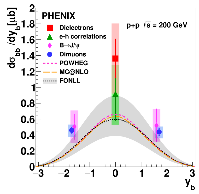
Figure 27: Rapidity density $d\sigma_{b\bar{b}}/dy_{b}$ in $p$+$p$ collisions at $\sqrt{s}=200$ GeV measured in PHENIX via various channels compared to theoretical calculations. Here $y_{b}$ is the rapidity of a $b$ quark.

The extracted cross sections using pythia and powheg are listed in Table. 5. The first two columns display the cross sections obtained by fitting data from the south and north muon arm at backward and forward rapidity, respectively. These values are then converted rapidity $d\sigma_{b\bar{b}}/dy$ at $y=-1.7$ and $y=+1.7$, corresponding to the average rapidity of the south and north muon arms.

Table 5: $\sigma_{b\bar{b}}$ from fit using different models. Only statistical uncertainties are shown.

	south	north	combined
pythia $\sigma_{b\bar{b}}$ [$\mu$b]	$3.71\pm 0.29$	$3.42\pm 0.35$	$3.59\pm 0.22$
powheg $\sigma_{b\bar{b}}$ [$\mu$b]	$3.94\pm 0.31$	$3.94\pm 0.40$	$3.94\pm 0.25$
average $\sigma_{b\bar{b}}$ [$\mu$b]	$3.82\pm 0.30$	$3.65\pm 0.38$	$3.75\pm 0.24$

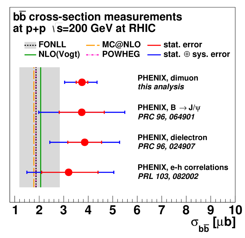
Figure 28: Bottom cross section $\sigma_{b\bar{b}}$ in $p$+$p$ collisions at $\sqrt{s}=200$ GeV measured at RHIC via various channels compared to NLL and NLO calculations. The gray band represents the systematic uncertainty in the FONLL calculation.

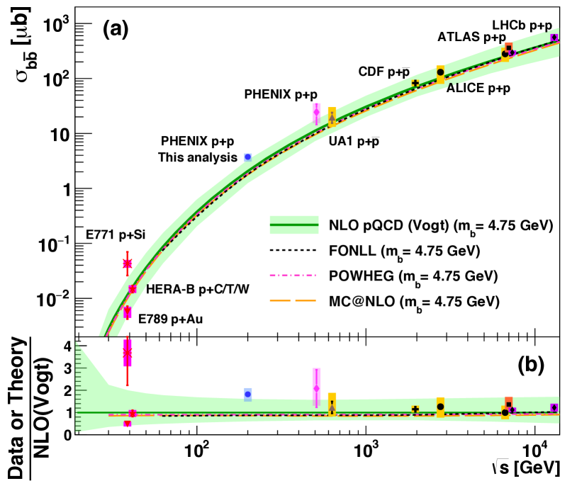
Figure 29: Bottom cross section $\sigma_{b\bar{b}}$ as a function of $\sqrt{s}$. Uncertainties due to rapidity extrapolation are not included in the LHCb measurements. Measured cross sections are compared to NLL and NLO calculations.

The results are shown in Fig. 27 and compared to other PHENIX bottom-cross-section measurements via various channels ($B\rightarrow J/\psi$ Aidala et al. (2017b), dielectrons Adare et al. (2017a), $e$-$h$ correlations Adare et al. (2009b)), and differential cross sections computed using fixed-order-plus-next-to-leading-log (FONLL) Cacciari et al. , mcnlo Frixione et al. (b) and powheg Frixione et al. (a). In all three calculations, we adopted the “standard” value of $m_{b}=4.75$ GeV/$c^{2}$ Vogt (2008). This choice of the bottom quark mass is mainly motivated by the mass of $\Upsilon(1S)$. It has been shown in previous studies that the NLO pQCD calculations with this standard value of $m_{b}$ can reproduce the $p$$+A$ and $\pi$+$p$ bottom cross sections at low energies fairly well to within large experimental and theoretical uncertainties Vogt (2003). The large theoretical uncertainties arise from the renormalization and factorization scale, bottom quark mass and PDF choices. We observe that the model dependence on the differential bottom cross section as a function of rapidity is small ($<10$%); it is mainly due to the uncertainties in the PDFs. The shaded band correspond to theoretical uncertainties estimated using a FONLL calculation, which includes uncertainties on the renormalization and factorization scales, bottom quark mass (varied between $4.5$ and $5.0$ GeV/$c^{2}$), and PDFs, added in quadrature. The measurements at $\sqrt{s}=$200 GeV tend to prefer the upper limit of this uncertainty band.

The measurements using the two muon arms can be combined to give a more precise measurement of the total bottom cross section, $\sigma_{b\bar{b}}[\mu b]=3.75\pm 0.24(stat)\pm^{0.35}_{0.50}(syst)\pm 0.45(global)$, which is the most precise measurement of the bottom cross section at $\sqrt{s}=200$ GeV to date. In Fig. 28, our measurement is compared to all other RHIC measurements.

As can be seen from Figs. 27 and 28, all RHIC bottom-cross-section measurements are remarkably consistent with each other. We compare to the total cross sections from various next-to-leading order (NLO) or next-to-leading logarithmic (NLL) calculations, including the NLO calculation from Ref. Vogt (2008), again using the value $m_{b}=4.75$ GeV/$c^{2}$ for the bottom quark mass. The total bottom cross section is around a factor of two higher than all theoretical calculations with $m_{b}=4.75$ GeV/$c^{2}$.

These measurements can be compared to the global trend of the $b\bar{b}$ cross section as a function of $\sqrt{s}$ Alexopoulos et al. (1999); Jansen et al. (1995); Abt et al. (2006); Acosta et al. (2005a); Abelev et al. (2013); Albajar et al. (1991); Aaij et al. (2017); Aidala et al. (2017c); Abelev et al. (2014); Aad et al. (2012), as shown in Fig. 29. Interestingly, the variation of different theoretical calculations is less than 8% despite spanning 5 orders of magnitude in cross section and 3 orders of magnitude in beam energy. At beam energies larger than 2 TeV, the data points from the Tevatron and LHC are in good agreement with the central values of the theoretical calculations, in contrast to measurements at $\sqrt{s}=200$ GeV at RHIC. Following the unconstrained averaging procedure adopted by the PDG  Patrignani et al. (2016), the weighted average of the $\sigma_{b\bar{b}}$ measurements at RHIC is $3.8\pm 0.5\ \mu b$, and is $>3\sigma$ higher than the theoretical central values (see Fig. 28). This may suggest that while the current central/default settings of these theoretical calculations may reasonably describe bottom cross sections at high beam energies, they fail to describe the cross section at $\sqrt{s}=200$ GeV.

An input bottom quark mass $m_{b}=4.12\pm 0.11$ GeV/$c^{2}$ is required for powheg to reproduce the bottom cross section measured at $\sqrt{s}=200$ GeV. This mass is significantly lower than the pole mass of the bottom quark, 4.78 GeV/$c^{2}$ Patrignani et al. (2016), hence it is unlikely that this discrepancy can be explained solely by the uncertainty in the bottom quark mass.

This measurement indicates that an effect which is more visible at lower beam energies may still be missing in current theoretical calculations. Future measurements at beam energies between $\sim 10$ GeV and $\sim 1000$ GeV with higher precision should help shed light on this issue.

IX.1 Drell-Yan differential cross section

The fully corrected $\mu\mu$ pair cross section from the Drell-Yan process in the pair rapidity region $1.2<|y^{\mbox{$\mu\mu$}}|<2.2$, as a function of mass, and a function of $p_{T}$ for pairs in the mass region $4.8<m$ [GeV/$c^{2}$ ]$<8.2$ are shown in Figs. 30 and 31, respectively. The kinematic region covered by the measurement corresponds to a Bjorken-$x$ value of $\approx 5\times 10^{-3}$. The measured differential Drell-Yan cross section at forward and backward rapidities are consistent with each other.

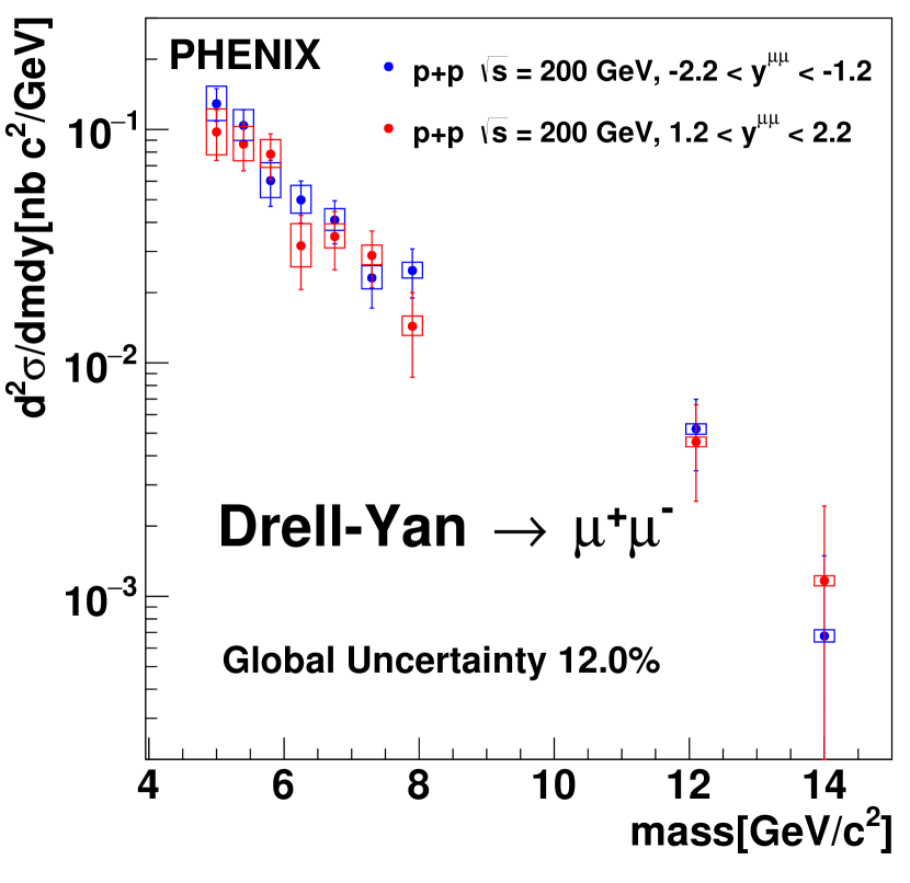
Figure 30: The corrected $\mu\mu$ yield from Drell-Yan in pair rapidity region $1.2<|y^{\mbox{$\mu\mu$}}|<2.2$ as a function or pair mass. Results are shown separately for the south and north muon arms.

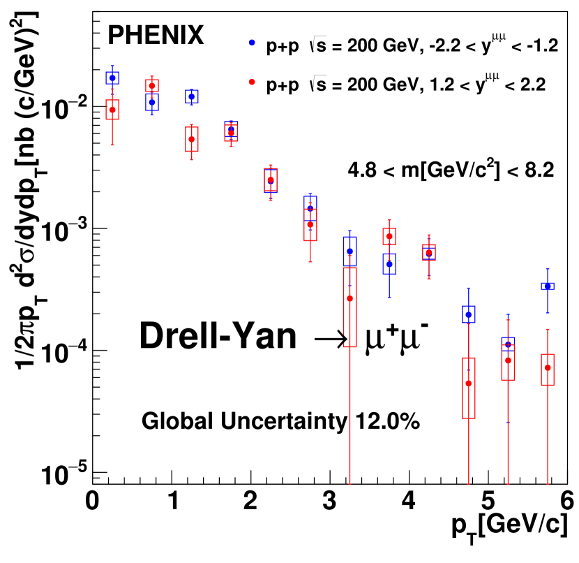
Figure 31: The corrected $\mu\mu$ yield from Drell-Yan in pair rapidity region $1.2<|y^{\mbox{$\mu\mu$}}|<2.2$ and mass region $4.8<m<8.2$ GeV/$c^{2}$ as a function of pair $p_{T}$. Results are shown separately for the south and north muon arms.

We combine the measurements from the two rapidity regions. The mass spectrum is then compared with NLO calculations from Vitev Neufeld et al. (2011) and Qiu J. et al Fai et al. (2005) in Fig. 32. Both calculations adopt the factorization approach where higher orders are evaluated order-by-order in perturbation theory. Within experimental uncertainties, the data are well reproduced by NLO calculations. The $p_{T}$ spectrum of Drell-Yan muon pairs in the mass region 4.8–8.2 GeV/$c^{2}$ is shown in Fig. 33 and compared to pythia, where the intrinsic $k_{T}$ is tuned from the procedure described in VII.1.4, and normalized from the fitting procedure as documented in the above text. We find that an intrinsic $k_{T}$ of 1.1 GeV/$c$ and a k-factor of 1.23 best describe the data. To date this is the first Drell-Yan measurement at RHIC energies. As Drell-Yan is a common background to various physics processes involving dileptons, the presented data may give a constraint for the background estimation of such measurements. The Drell-Yan cross section as a function of invariant mass and $p_{T}$ can also provide constraints on the unpolarized transverse-momentum-dependent parton distribution functions (TMD PDFs), which is of critical importance to understanding the internal structure of the proton. This measurement gives input to a previously unexplored phase space and serves as a solid baseline for future measurements.

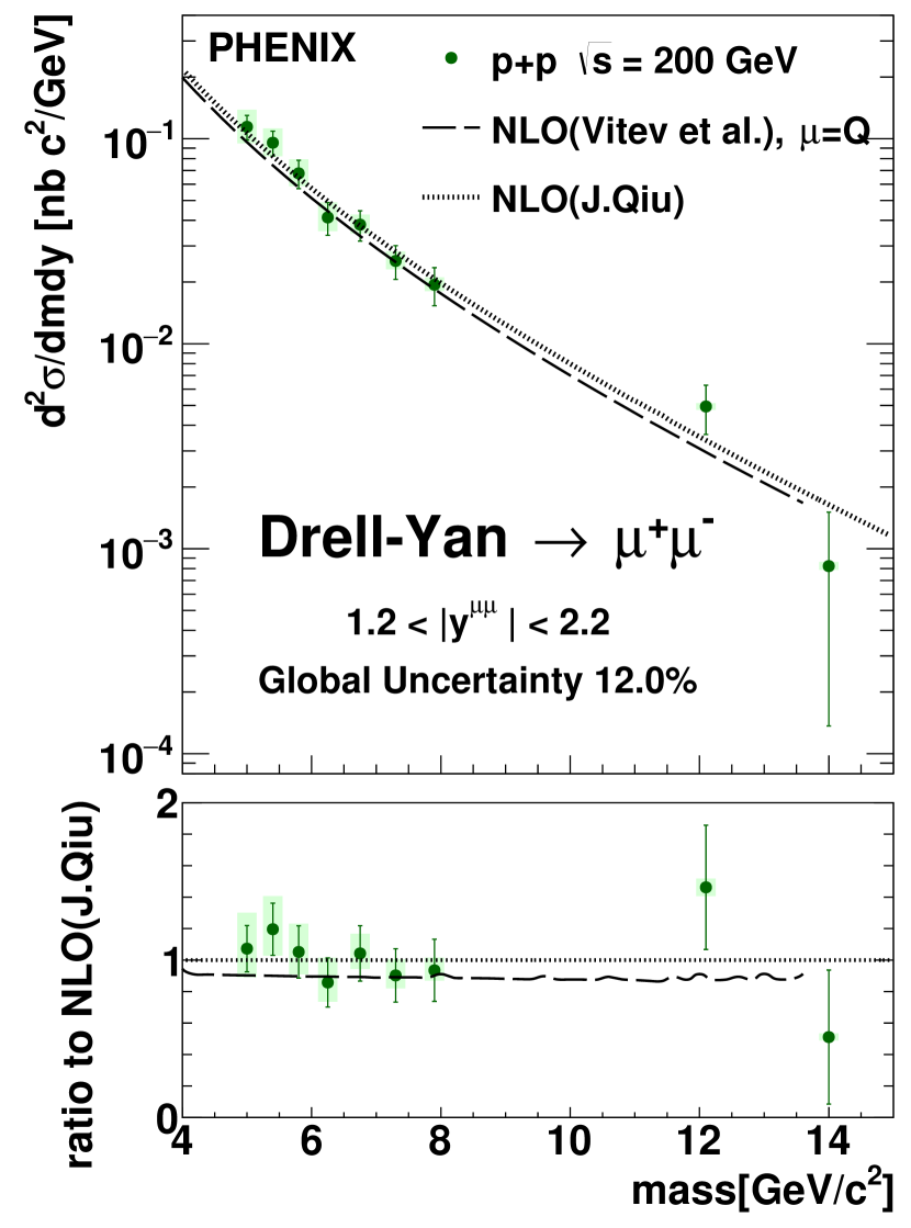
Figure 32: Panel (a) shows the corrected $\mu\mu$ yield from Drell-Yan in pair rapidity region $1.2<|y^{\mbox{$\mu\mu$}}|<2.2$. Data are compared to NLO calculations. Panel (b) gives the ratio of the data to one of the NLO calculations.

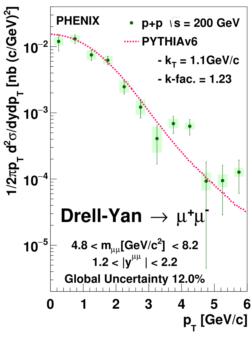
Figure 33: The corrected $\mu\mu$ yield from Drell-Yan in pair rapidity region $1.2<|y^{\mbox{$\mu\mu$}}|<2.2$ and mass region $4.8<m<8.2$ GeV/$c^{2}$ as a function of pair $p_{T}$. Data are compared pythia calculations under settings used for this analysis.

X Summary

We present $\mu\mu$ pair measurements from open heavy flavor decays and the Drell-Yan mechanism in $p$+$p$ collisions at $\sqrt{s}=200$ GeV.

Invariant yields of $\mu\mu$ pairs from $c\bar{c}$ and $b\bar{b}$ are measured as a function of $\Delta\phi$ and $p_{T}$ and compared to different models, pythia and powheg. Within experimental uncertainties, the azimuthal opening angle and pair $p_{T}$ distributions from $b\bar{b}$ are well described by these models. For $c\bar{c}$, the data favor the pythia description, while the powheg calculations predict a systematically higher yield than pythia at smaller opening angles in the probed kinematic region.

We find that the high mass like-sign pairs are dominated by decays from open bottom, which provides a strong constraint to the bottom cross section. The measured total bottom cross section is consistent with RHIC measurements at the same energy, and is around a factor of two higher than the central value of NLL and NLO calculations with an input bottom quark mass of $m_{b}=4.75$ GeV/$c^{2}$.

The Drell-Yan cross section as a function of mass in 4.8–15.0 GeV/$c^{2}$ is presented and compared to NLO calculations from Vitev and Qiu. Within uncertainties we find good agreement between NLO calculations and data. The Drell-Yan $p_{T}$ cross section in the mass region 4.8–8.2 GeV/$c^{2}$ is also presented, along with the pythia tune that best describes the data.

Appendix A DETAILED DESCRIPTION OF SIMULATION FRAMEWORKS

Details of the two simulation chains used in this analysis, namely the default PHENIX simulation framework and the fastMC, are discussed in the following. The flowchart shown in Fig. 34 summarizes a comparison between the data reconstruction framework and the two simulation chains.

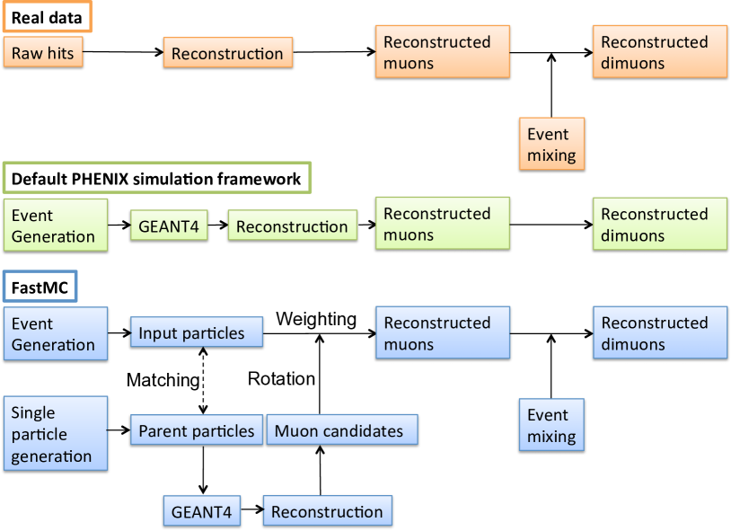
Figure 34: Flow chart of the analysis chain of the dimuon reconstruction for real data, default PHENIX simulation framework, and FastMC framework.

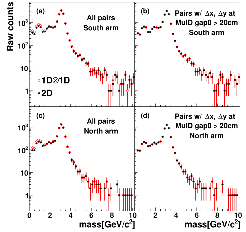
Figure 35: The mass spectra of MuIDLL1-1D triggered data for the (a,b) south arm and (c,d) the north arm are shown separately. Open circles are pairs in which both associated tracks satisfy the MuIDLL1-1D condition, while closed circles are pairs in which the associated tracks satisfy the MuIDLL1-2D condition. Panels (a,c) show all pairs, while the panels (b,d) show only pairs with a spatial separation exceeding 20 cm at MuID gap 0.

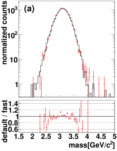
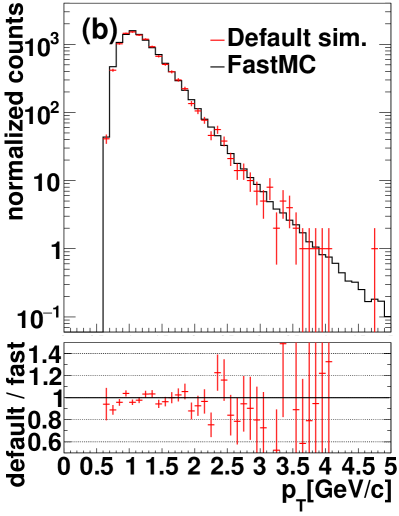
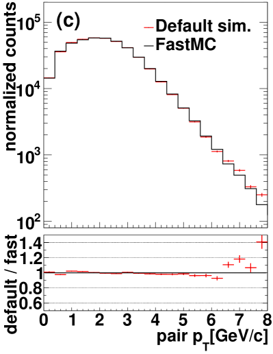
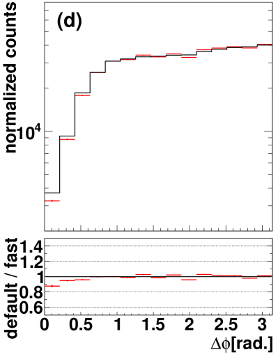
Figure 36: Comparison of distributions from FastMC and default PHENIX simulation framework. (a) mass spectrum of $J/\psi$ muon pairs; (b) single $p_{T}$ spectrum of muons from $\pi^{\pm}$ and $K^{\pm}$ with realistic input $p_{T}$ spectra; (c) pair $p_{T}$ spectrum of muon pairs from $b\bar{b}$; (d) $\Delta\phi$ of muon pairs from $b\bar{b}$.

A.1 Default PHENIX simulation framework

The default PHENIX simulation is based on a detailed geant4 Agostinelli et al. (2003) implementation of the muon arms. This framework takes into account the detector’s geometrical acceptance and all inefficiencies from dead channels. To account for variations of detector performance during the data taking period, the data are split into run groups with similar performance. For each group a map of dead channels is created for the MuTr. The simulation randomly selects these maps according to the sampled luminosity for each run group.

Muon pairs from physical sources are simulated with a $z$-vertex distribution taken from MB $p$+$p$ data. Once the pairs are processed through the detector simulation, they are reconstructed using the same procedure and filtered with the same cuts as used for real data. Thus, all detector effects including acceptance, dead areas, track reconstruction, and analysis cuts are taken properly into account.

Because the analyzed data are triggered with the MuIDLL1-2D trigger, the effects of the trigger also need to be accounted for. To achieve this, we apply an offline software trigger to all simulated tracks, which is an exact replication of the online hardware MuIDLL1-1D trigger. We require that both tracks of a pair fulfill the MUIDLL1-1D trigger condition. Here we make use of the fact that after enforcing a spatial separation of 20 cm between two MuID tracks, the MuIDLL1-2D pair trigger is reduced to a logical AND of the MuIDLL1-1D single track triggers. The separation cut necessary to achieve this factorization was determined from experimental data. In Fig. 35(a,c) a $\sim$20–30% difference between the mass distribution from data triggered with the MuIDLL1-2D and the data requiring each track fulfills the MuIDLL1-1D is visible at low masses. Once the separation cut is applied the difference disappears, as seen in panels (b) and (d).

A.2 FastMC

In spite of the large hadron rejection power ($\sim 1/1000$) of the muon arms, a significant fraction of the reconstructed muons are from decays of light-flavor mesons ($\pi^{\pm}$, $K^{\pm}$, and $K^{0}$). Using the default Monte-Carlo to simulate these pairs is unpractical, because for every 1,000,000 generated pairs of particles in the detector acceptance, only one muon pair would be reconstructed from the simulation. In the FastMC approach we separate the generation of particles that result in reconstructed $\mu\mu$ pairs from the simulation of the detailed detector response to an individual particle. The FastMC proceeds in four steps: (i) generation of a repository of possible detector responses to an individual particle using the default simulation framework, (ii) creation of events with multiple muons from the sources discussed in Sec. IV, here the repository created in step (i) is used to determine the detector response, (iii) weighting each reconstructed muon with the appropriate probability for being reconstructed and not rejected by the analysis cuts, and (iv) finally forming muon pairs and calculating their mass, $p_{T}$ and azimuthal opening angle.

A.2.1 Detector response to individual particles

For each particle species ($\pi^{\pm}$, $K^{\pm}$, $K^{0}$, and $\mu^{\pm}$) $\sim 10^{9}$ particles were simulated. All particles are propagated through the full geant4 simulation and reconstruction chain. Light hadrons ($\pi^{\pm}$, $K^{\pm}$, and $K^{0}$) may give rise to a reconstructed muon either via (i) decaying to a muon in flight (decay muons), or (ii) penetrating all absorber layers (punch-through hadrons). The contribution from protons is negligible ($<1\%$) compared to kaons and pions and hence neglected in this study.

These parent particles are generated with flat distribution in momentum $p$ and polar angle $\theta$, and uniform distribution in $\phi$. Simulations are performed in three uniform $z$-vertex regions, $(-22.5,-17.5~{}{\rm cm})$, $(-2.5,2.5~{}{\rm cm})$, and $(17.5,22.5~{}{\rm cm})$, to account for variances in detector response along $z_{\rm vtx}$. Improvements by expanding to full collision $z_{\rm vtx}$ coverage in simulations is expected to be minimal(see Sec. VII.1.8). All reconstructed variables are stored along with the generated vertex and parent momentum information. These muon candidates are grouped into pools according to parent particle species and parent $p$ and $\theta$, where $p$ and $\theta$ ranges from 2 to 32 GeV/$c$ and 0 to 0.8 radians respectively, which covers the kinematic region relevant for this analysis. One single pool covers the kinematic region $\Delta p\times\Delta\theta=0.1\times 0.02$ [GeV/$c$ rad]. The minimum number of muon candidates in one pool is $\sim 10$. These pools are used as repository for the possible detector response to parent particles in the subsequent steps of the FastMC.

A.2.2 Events with reconstructed muons

To create an event with reconstructed muons, we first generate events of particles as discussed in Sec. IV.2. For each event the list of particles is filtered so that only $\pi^{\pm}$, $K^{\pm}$, $K^{0}$, and $\mu^{\pm}$ in the vicinity of the muon arm acceptance are kept, and the momentum information of these particles is stored. We will refer to these particles as input particles.

A given input particle is matched to a pool of muon candidates in the repository for that particle species, and the input particle’s $p$ and $\theta$. We randomly choose one muon candidate from the pool and use the reconstructed variables from that muon candidate for the input particle. The repository pools were generated from parent particles with a uniform $\phi$ distribution. While the input particles are matched to the muon candidate in parent $p$ and $\theta$, they are not matched in $\phi$. We therefore rotate all reconstructed variables in the azimuthal plane from the $\phi$ of the parent of the muon candidate to the $\phi$ of input particle.

At this point we have created a reconstructed muon with all the characteristics that could have resulted from propagating the input particle through the default simulation framework. In particular, because the matching of input particles to muon candidates is completely random, the relative contributions and momentum distribution of decay muons and punch-through hadrons are properly accounted for. This procedure is repeated for all input particles in an event.

A.2.3 Weighting each reconstructed muon with its probability

So far each input particle leads to a reconstructed muon. This does not take into account the hadron rejection of the muon arms and the reconstruction efficiencies. Rejection and efficiency are encapsulated in weighting factors that are applied to each reconstructed muon. We factorize the weight into two components weight_reco and weight_ϕ, which are discussed in the following. The final weight is calculated as:

$${\rm weight}={\rm weight}_{\rm reco}\times{\rm weight}_{\phi}.$$ (23)

Weighting in $p$ and $\theta$

The survival probability of a decay muon is highly dependent on the momentum of the muon, as well as the amount of material it traverses in the absorber, which in turn is dependent on the input particle’s momentum $p$ and the polar angle $\theta$. We associate a weighting factor weight${}_{\rm reco}(p,\theta,z)$ to each muon candidate. This factor is the probability that an input particle with momentum $p$ and polar angle $\theta$, produced at vertex $z$, results in the reconstructed muon candidate, averaged over $\phi$. The weight is computed by dividing the number of reconstructed muons in each pool by the number of parent particles generated to create the corresponding pool.

Weighting in $\phi$

In addition to weight${}_{\rm reco}(p,\theta,z)$, we also need to weight in $\phi$ direction, weight_ϕ, to account for the $\phi$ dependent relative survival probability and reconstruction efficiency. These mainly depend on the geometry of the MuTr, thus the weighting factors are determined by a combination of variables $(\phi^{\rm MuTr},p_{T}^{\rm MuTr},p_{z}^{\rm MuTr})$, which are the azimuthal position, transverse momentum, and longitudinal momentum evaluated at MuTr Station 1. To determine weight_ϕ, we generate single muons with a realistic momentum distribution and propagate these muons through the default simulation framework. Because the overall survival probability is factored into weight_reco, weight_ϕ is normalized by requiring the average value of weight_ϕ to be one, i.e.

$${\rm weight}_{\phi}(\phi^{\rm MuTr},p_{T}^{\rm MuTr},p_{z}^{\rm MuTr})$$

$$=\frac{N_{\rm reco}(\phi^{\rm MuTr},p_{T}^{\rm MuTr},p_{z}^{\rm MuTr})\int^{+\pi}_{-\pi}d\phi^{\rm MuTr}}{\int^{+\pi}_{-\pi}d\phi^{\rm MuTr}N_{\rm reco}(\phi^{\rm MuTr},p_{T}^{\rm MuTr},p_{z}^{\rm MuTr})}.$$ (24)

A.2.4 Constructing muon pairs

In each event all reconstructed muons are combined to pairs. The pair variables are constructed from the reconstructed muon information following the exact same procedure as in real data. The weighting factor for a muon pair is the product of the weighting factors of the two reconstructed muons:

$${\rm weight}_{12}={\rm weight}_{1}\times{\rm weight}_{2}.$$ (25)

This assumes that the pair reconstruction efficiency is a product of single track reconstruction efficiencies, which is true for tracks that are spatially separated in the MuTr and MuID. The latter is assured by the pair cuts we apply.

To estimate the accuracy of the FastMC, which is used to simulate muon-hadron and hadron-hadron pairs, we propagate $\mu\mu$ pairs and single hadrons through the default simulation framework and FastMC and compared the resulting distributions. We find that the mass resolution, $\Delta\phi$, single and pair $p_{T}$ distributions are well reproduced by the FastMC (see Fig. 36). Small discrepancies are observed in the azimuthal opening angle distribution $\Delta\phi$ between the two muons for small $\Delta\phi$. This is likely due to the $\phi$ weighting procedure. The related systematic uncertainties will be discussed in Sec. VII.

Appendix B WEIGHTED AVERAGE OF SOUTH AND NORTH MUON ARM RESULTS

We calculate a weighted average of the results from the south and north muon arms to obtain final results. The same method of weighting is used for all combined quantities, including the bottom cross section, angular and momentum distributions for $c\bar{c}$ and $b\bar{b}$ muon pairs, and the Drell-Yan $p_{T}$ and mass distributions. Each quantity $\Gamma$, which can represent a yield in a given bin or a cross section, is calculated as a weighted average of the measured values $\Gamma_{S}$ and $\Gamma_{N}$ using the south and north arm respectively, according to:

$$\Gamma=\frac{w_{S}\Gamma_{S}+w_{N}\Gamma_{N}}{w_{{\rm tot}}}.$$ (26)

The weights for the south and north arms, $w_{j}$ ($j=S,N$), are calculated from the inverse of the quadrature sum of statistical and uncorrelated systematic uncertainties, i.e. those systematic errors that are not common for the south and north measurements. Denoting $\sigma^{2}_{j,{\rm syst}}$, $\sigma^{2}_{j,{\rm uncorr}}$ and $\sigma^{2}_{j,{\rm corr}}$ as the total, uncorrelated, and correlated systematic uncertainties such that $\sigma^{2}_{j,{\rm syst}}=\sigma^{2}_{j,{\rm uncorr}}+\sigma^{2}_{j,{\rm corr}}$, the weights $w_{j}$ are given by the relation:

$$w_{j}=\frac{1}{\sigma^{2}_{j,{\rm stat}}+\sigma^{2}_{j,{\rm uncorr}}}.$$ (27)

The weight $w_{{\rm tot}}$ is the sum of the weights for south and north arm, i.e. $w_{{\rm tot}}=w_{S}+w_{N}$. For the statistical uncertainties on the weighted average we quote:

$$\sigma^{2}_{{\rm stat}}=\frac{w_{S}^{2}\sigma^{2}_{S,{\rm stat}}+w_{N}^{2}\sigma^{2}_{N,{\rm stat}}}{w_{{\rm tot}}^{2}}.$$ (28)

The systematic uncertainties that are fully correlated between south and north arms are treated separately from uncorrelated systematic uncertainties as specified below:

$$\sigma^{2}_{{\rm syst}}= \frac{w_{S}^{2}\sigma^{2}_{S,{\rm uncorr}}+w_{N}^{2}\sigma^{2}_{N,{\rm uncorr}}}{w_{{\rm tot}}^{2}}$$

$$+\frac{(w_{S}\sigma_{S,{\rm corr}}+w_{N}\sigma_{N,{\rm corr}})^{2}}{w_{{\rm tot}}^{2}},$$ (29)

These systematic uncertainties are calculated separately for the upper and lower boundaries.

Appendix C SIMULATION PARAMETERS

Table 6: Parameters used in pythia Tune A simulation.

Parameter	Setting	Description
MSEL	1	Turn on all QCD processes
PARP(67)	4.0	Set hard scattering scale $\mu^{2}$
PARP(82)	2.0	Turn off $p_{T}$ for multiparticle interactions
PARP(84)	0.4	Radius of core Gaussian matter
PARP(85)	0.9	Probability that two gluons are
		produced with colors connected
		to the nearest neighbors
PARP(86)	0.95	Probability that two gluons
		are produced with PARP(85)
		conditions or closed loop
PARP(89)	1800	Reference energy scale of the turn-off $p_{T}$
PARP(90)	0.25	Energy dependence of the turn-off $p_{T}$
PARP(91)	1.5	Primordial $k_{T}$ Gaussian width
CKIN(3)	1.5	Lower cutoff on $\hat{p}_{\perp}$
MSTP(51)	7	CTEQ 5L, leading order PDF

Table 7: Parameters used in pythia Drell-Yan simulations.

Parameter	Setting	Description
MSEL	0	Select subprocesses manually
MSTP(43)	3	Select Drell-Yan process
		Complete $Z^{0}/\gamma^{*}$ structure
MSUB(1)	1	Turn on $q+\bar{q}$ $\rightarrow$ $Z^{0}/\gamma^{*}$ $\rightarrow$ $\mu^{+}\mu^{-}$
MSTP(91)	1	Gaussian primordial $k_{T}$
PARP(91)	$1.1$	Gaussian width of $k_{T}$ in GeV/$c$
MSTP(33)	1	Inclusion of k-factors in
		hard cross sections
MSTP(32)	4	Use $Q^{2}=\hat{s}^{2}$
CKIN(1)	0.5	Lower cutoff on $\hat{m}=\sqrt{\hat{s}}$
CKIN(2)	-1	Upper cutoff on $\hat{m}=\sqrt{\hat{s}}$
CKIN(3)	0.0	Lower cutoff on $\hat{p}_{\perp}$
CKIN(4)	-1	Upper cutoff on $\hat{p}_{\perp}$
MSTP(51)	7	CTEQ 5L, leading order PDF

Appendix D DATA TABLES

Table 8: The differential yield $dN/d\phi$ of unlike-sign muon pairs from charm with mass 1.5–2.5 GeV/$c^{2}$ in the ideal muon arm acceptance, as a function of the pair azimuthal opening angle.

$|\phi_{\mu,1}$–$\phi_{\mu,2}|$	$dN/d\phi$	stat. error	sys. error (type B)	sys. error (type C)
[rad]	$10^{-9}\times$[rad-1]	$10^{-9}\times$[rad-1]	$10^{-9}\times$[rad-1]	$10^{-9}\times$[rad-1]
0–$\frac{\pi}{15}$	-0.136	0.199	${}^{+3.3\times 10^{-2}}_{-4.3\times 10^{-2}}$	$1.6\times 10^{-2}$
$\frac{\pi}{15}$–$\frac{2\pi}{15}$	-1.43 $\times 10^{-2}$	0.130	${}^{+4.87\times 10^{-2}}_{-3.22\times 10^{-2}}$	1.7 $\times 10^{-3}$
$\frac{2\pi}{15}$–$\frac{3\pi}{15}$	0.456	0.237	${}^{+0.165}_{-0.174}$	5.5$\times 10^{-2}$
$\frac{3\pi}{15}$–$\frac{4\pi}{15}$	0.238	0.280	${}^{+0.334}_{-0.298}$	2.9$\times 10^{-2}$
$\frac{4\pi}{15}$–$\frac{5\pi}{15}$	1.08	0.41	${}^{+0.57}_{-0.51}$	0.13
$\frac{5\pi}{15}$–$\frac{6\pi}{15}$	0.443	0.579	${}^{+0.792}_{-0.685}$	5.3$\times 10^{-2}$
$\frac{6\pi}{15}$–$\frac{7\pi}{15}$	3.34	0.71	${}^{+0.94}_{-0.85}$	0.40
$\frac{7\pi}{15}$–$\frac{8\pi}{15}$	5.02	0.87	${}^{+0.95}_{-0.85}$	0.60
$\frac{8\pi}{15}$–$\frac{9\pi}{15}$	7.09	0.93	${}^{+0.83}_{-0.77}$	0.85
$\frac{9\pi}{15}$–$\frac{10\pi}{15}$	7.97	0.97	${}^{+0.77}_{-0.73}$	0.96
$\frac{10\pi}{15}$–$\frac{11\pi}{15}$	6.69	1.05	${}^{+0.82}_{-0.80}$	0.80
$\frac{11\pi}{15}$–$\frac{12\pi}{15}$	7.70	1.11	${}^{+0.98}_{-0.96}$	0.92
$\frac{12\pi}{15}$–$\frac{13\pi}{15}$	10.2	1.1	${}^{+1.3}_{-1.3}$	1.2
$\frac{13\pi}{15}$–$\frac{14\pi}{15}$	7.95	1.09	${}^{+1.28}_{-1.27}$	0.95
$\frac{14\pi}{15}$–$\pi$	6.15	1.21	${}^{+1.13}_{-1.12}$	0.74

Table 9: The differential yield $dN/d\phi$ of like-sign muon pairs from bottom with mass 3.5–10.0 GeV/$c^{2}$ in the ideal muon arm acceptance, as a function of the pair azimuthal opening angle.

$|\phi_{\mu,1}$–$\phi_{\mu,2}|$	$dN/d\phi$	stat. error	sys. error (type B)	sys. error (type C)
[rad]	$10^{-9}\times$[rad-1]	$10^{-9}\times$[rad-1]	$10^{-9}\times$[rad-1]	$10^{-9}\times$[rad-1]
$\frac{4\pi}{12}$–$\frac{5\pi}{12}$	$8.36\times 10^{-2}$	$3.47\times 10^{-2}$	${}^{+9.2\times 10^{-3}}_{-9.2\times 10^{-3}}$	$1.0\times 10^{-2}$
$\frac{5\pi}{12}$–$\frac{6\pi}{12}$	$5.74\times 10^{-2}$	$2.72\times 10^{-2}$	${}^{+3.5\times 10^{-3}}_{-3.6\times 10^{-3}}$	$6.9\times 10^{-3}$
$\frac{6\pi}{12}$–$\frac{7\pi}{12}$	0.274	$6.6\times 10^{-2}$	${}^{+1.1\times 10^{-2}}_{-1.2\times 10^{-2}}$	$3.3\times 10^{-2}$
$\frac{7\pi}{12}$–$\frac{8\pi}{12}$	0.531	$9.6\times 10^{-2}$	${}^{+2.3\times 10^{-2}}_{-2.8\times 10^{-2}}$	$6.4\times 10^{-2}$
$\frac{8\pi}{12}$–$\frac{9\pi}{12}$	1.13	0.14	${}^{+5\times 10^{-2}}_{-9\times 10^{-2}}$	0.14
$\frac{9\pi}{12}$–$\frac{10\pi}{12}$	1.51	0.18	${}^{+9\times 10^{-2}}_{-0.18}$	0.18
$\frac{10\pi}{12}$–$\frac{11\pi}{12}$	1.87	0.22	${}^{+0.16}_{-0.30}$	0.22
$\frac{11\pi}{12}$–$\pi$	1.94	0.24	${}^{+0.21}_{-0.41}$	0.23

Table 10: The differential yield $dN/dp_{T}$ of unlike-sign muon pairs from bottom with mass 1.5–2.5 GeV/$c^{2}$ in the ideal muon arm acceptance, as a function of the pair transverse momentum.

$p_{T}$	$dN/dp_{T}$	stat. error	sys. error (type B)	sys. error (type C)
[GeV/$c$]	$10^{-9}\times$[$c$/GeV]	$10^{-9}\times$[$c$/GeV]	$10^{-9}\times$[$c$/GeV]	$10^{-9}\times$[$c$/GeV]
0–0.2	1.02	0.73	${}^{+0.59}_{-0.59}$	0.12
0.2–0.4	3.97	1.05	${}^{+1.32}_{-1.31}$	0.48
0.4–0.6	8.16	1.17	${}^{+1.37}_{-1.36}$	0.98
0.6–0.8	8.91	1.19	${}^{+1.22}_{-1.21}$	1.07
0.9-1.0	5.89	1.08	${}^{+0.92}_{-0.91}$	0.71
1.0–1.2	6.31	1.00	${}^{+0.75}_{-0.73}$	0.76
1.2–1.4	5.58	0.90	${}^{+0.66}_{-0.64}$	0.67
1.4–1.6	6.91	0.84	${}^{+0.62}_{-0.60}$	0.83
1.6–1.8	5.15	0.75	${}^{+0.58}_{-0.53}$	0.62
1.8–2.0	3.46	0.67	${}^{+0.53}_{-0.49}$	0.42
2.0–2.4	1.90	0.41	${}^{+0.50}_{-0.43}$	0.23
2.4–2.8	0.761	0.309	${}^{+0.408}_{-0.370}$	$9.1\times 10^{-2}$
2.8–3.2	$-5.97\times 10^{-2}$	0.239	${}^{+0.353}_{-0.298}$	$7.2\times 10^{-3}$
3.2–3.6	$5.02\times 10^{-2}$	0.203	${}^{+0.259}_{-0.242}$	$6.0\times 10^{-3}$
3.6–4.4	0.206	0.102	${}^{+0.135}_{-0.118}$	$2.5\times 10^{-2}$
4.4–5.2	$8.18\times 10^{-2}$	$8.03\times 10^{-2}$	${}^{+6.77\times 10^{-2}}_{-5.64\times 10^{-2}}$	$9.8\times 10^{-3}$

Table 11: The differential yield $dN/dp_{T}$ of like-sign muon pairs from bottom with mass 3.5–10.0 GeV/$c^{2}$ in the ideal muon arm acceptance, as a function of the pair transverse momentum.

$p_{T}$	$dN/dp_{T}$	stat. error	sys. error (type B)	sys. error (type C)
[GeV/$c$]	$10^{-9}\times$[$c$/GeV]	$10^{-9}\times$[$c$/GeV]	$10^{-9}\times$[$c$/GeV]	$10^{-9}\times$[$c$/GeV]
0–0.5	0.199	$5.7\times 10^{-2}$	${}^{+2.7\times 10^{-2}}_{-5.0\times 10^{-2}}$	$2.4\times 10^{-2}$
0.5–1.0	0.576	$9.2\times 10^{-2}$	${}^{+5.6\times 10^{-2}}_{-0.122}$	$6.9\times 10^{-2}$
1.0–1.5	0.754	$9.9\times 10^{-2}$	${}^{+6.1\times 10^{-2}}_{-0.126}$	$9.0\times 10^{-2}$
1.5–2.0	0.777	$9.5\times 10^{-2}$	${}^{+5.0\times 10^{-2}}_{-9.6\times 10^{-2}}$	$9.3\times 10^{-2}$
2.0–2.5	0.536	$7.8\times 10^{-2}$	${}^{+3.3\times 10^{-2}}_{-5.8\times 10^{-2}}$	$6.4\times 10^{-2}$
2.5–3.0	0.376	$6.5\times 10^{-2}$	${}^{+2.0\times 10^{-2}}_{-3.1\times 10^{-2}}$	$4.5\times 10^{-2}$
3.0–3.5	0.230	$4.9\times 10^{-2}$	${}^{+1.1\times 10^{-2}}_{-1.8\times 10^{-2}}$	$2.8\times 10^{-2}$
3.5–4.0	0.199	$4.3\times 10^{-2}$	${}^{+8\times 10^{-3}}_{-1.0\times 10^{-2}}$	$2.4\times 10^{-2}$
4.0–4.5	$9.05\times 10^{-2}$	$2.93\times 10^{-2}$	${}^{+3.8\times 10^{-3}}_{-4.9\times 10^{-3}}$	$1.09\times 10^{-2}$
4.5–5.0	$2.37\times 10^{-2}$	$1.75\times 10^{-2}$	${}^{+1.4\times 10^{-3}}_{-1.4\times 10^{-3}}$	$2.9\times 10^{-3}$

Table 12: The differential Drell-Yan cross section $\frac{d^{2}\sigma}{dmdy}$ as a function of the muon pair mass, where the muon pair rapidity $|y_{\mu\mu}|$ is between 1.2 and 2.2.

$m_{\mu\mu}$	$\frac{d^{2}\sigma}{dmdy}$	stat. error	sys. error (type B)	sys. error (type C)
[GeV/$c^{2}$]	[pb $c^{2}$/GeV]	[pb $c^{2}$/GeV]	[pb $c^{2}$/GeV]	[pb $c^{2}$/GeV]
5	114	16	${}^{+24}_{-19}$	14
5.4	95.6	13.3	${}^{+16.8}_{-13.4}$	11.5
5.8	67.8	10.7	${}^{+11.6}_{-9.1}$	8.1
6.25	41.3	7.5	${}^{+7.6}_{-5.9}$	5.0
6.75	38.1	6.5	${}^{+4.6}_{-3.6}$	4.6
7.3	25.3	4.8	${}^{+2.9}_{-2.3}$	3.0
7.9	19.4	4.1	${}^{+1.7}_{-1.4}$	2.3
12.1	4.94	1.33	${}^{+0.19}_{-0.19}$	0.59
14	0.823	0.686	${}^{+3.9\times 10^{-2}}_{-3.4\times 10^{-2}}$	$9.9\times 10^{-2}$

Table 13: The differential Drell-Yan cross section $\frac{1}{2\pi p_{T}}\frac{d^{2}\sigma}{dydp_{T}}$ as a function of the muon pair transverse momentum, where the muon pair mass $m_{\mu\mu}$ is between 4.8 and 8.2 GeV/$c^{2}$ and the muon pair rapidity $|y_{\mu\mu}|$ is between 1.2 and 2.2.

$p_{T}$	$\frac{1}{2\pi p_{T}}\frac{d^{2}\sigma}{dydp_{T}}$	stat. error	sys. error (type B)	sys. error (type C)
[GeV/$c$]	[pb ($c$/GeV)2]	[pb ($c$/GeV)2]	[pb ($c$/GeV)2]	[pb ($c$/GeV)2]
0.25	12.0	3.4	${}^{+1.9}_{-1.6}$	1.4
0.75	13.1	2.0	${}^{+1.8}_{-1.4}$	1.6
1.25	7.48	1.30	${}^{+1.42}_{-1.14}$	0.90
1.75	6.22	0.93	${}^{+1.00}_{-0.81}$	0.75
2.25	2.48	0.55	${}^{+0.59}_{-0.46}$	0.30
2.75	1.22	0.39	${}^{+0.37}_{-0.29}$	0.15
3.25	0.408	0.239	${}^{+0.206}_{-0.157}$	$4.9\times 10^{-2}$
3.75	0.688	0.198	${}^{+0.123}_{-0.103}$	$8.3\times 10^{-2}$
4.25	0.627	0.164	${}^{+8.4\times 10^{-2}}_{-7.1\times 10^{-2}}$	$7.5\times 10^{-2}$
4.75	$9.29\times 10^{-2}$	$8.84\times 10^{-2}$	${}^{+3.30\times 10^{-2}}_{-2.59\times 10^{-2}}$	$1.12\times 10^{-2}$
5.25	$9.47\times 10^{-2}$	$6.61\times 10^{-2}$	${}^{+2.28\times 10^{-2}}_{-1.98\times 10^{-2}}$	$1.14\times 10^{-2}$
5.75	0.127	$6.6\times 10^{-2}$	${}^{+1.9\times 10^{-2}}_{-1.9\times 10^{-2}}$	$1.5\times 10^{-2}$

References

- Christenson et al. (1970) J. H. Christenson, G. S. Hicks, L. M. Lederman, P. J. Limon, B. G. Pope, and E. Zavattini, “Observation of massive muon pairs in hadron collisions,” Phys. Rev. Lett. 25, 1523 (1970).
- Aubert et al. (1974) J. J. Aubert et al. (E598 Collaboration), “Experimental Observation of a Heavy Particle ,” Phys. Rev. Lett. 33, 1404 (1974).
- Adare et al. (2009a) A. Adare et al. (PHENIX Collaboration), “Dilepton mass spectra in + collisions at = 200 GeV and the contribution from open charm,” Phys. Lett. B 670, 313 (2009a).
- Adare et al. (2010) A. Adare et al. (PHENIX Collaboration), “Detailed measurement of the pair continuum in and Au+Au collisions at GeV and implications for direct photon production,” Phys. Rev. C 81, 034911 (2010).
- Adare et al. (2015) A. Adare et al. (PHENIX Collaboration), “Cross section for production via dielectrons in Au collisions at GeV,” Phys. Rev. C 91, 014907 (2015).
- Adare et al. (2016) A. Adare et al. (PHENIX Collaboration), “Dielectron production in AuAu collisions at =200 GeV,” Phys. Rev. C 93, 014904 (2016).
- Adare et al. (2017a) A. Adare et al. (PHENIX Collaboration), “Measurements of pairs from open heavy flavor in + and +A collisions at GeV,” Phys. Rev. C 96, 024907 (2017a).
- Adamczyk et al. (2014) L. Adamczyk et al. (STAR Collaboration), “Dielectron Mass Spectra from Au+Au Collisions at =200 GeV,” Phys. Rev. Lett. 113, 022301 (2014), [Addendum: Phys. Rev. Lett. 113, 049903 (2014)].
- (9) M. Cacciari, M. Greco, and P. Nason, “The spectrum in heavy flavor hadroproduction,” J. High Energy Phys. 05 (1998) 007.
- (10) T. Sjostrand, S. Mrenna, and P. Z. Skands, “PYTHIA 6.4 Phys. and Manual,” J. High Energy Phys. 05 (2006) 026 .
- Norrbin and Sjostrand (2000) E. Norrbin and T. Sjostrand, “Production and hadronization of heavy quarks,” Eur. Phys. J. C 17, 137 (2000).
- Frixione et al. (a) S. Frixione, P. Nason, and G. Ridolfi, “A Positive-weight next-to-leading-order Monte Carlo for heavy flavour hadroproduction,” (a), J. High Energy Phys. 09 (2007) 126.
- Frixione et al. (b) S. Frixione, P. Nason, and B. R. Webber, “Matching NLO QCD and parton showers in heavy flavor production,” (b), J. High Energy Phys. 08 (2003) 007.
- Vogt (2008) R. Vogt, “The Total charm cross-section,” Eur. Phys. J. ST 155, 213 (2008).
- Adare et al. (2011a) A. Adare et al. (PHENIX Collaboration), “Heavy Quark Production in and Energy Loss and Flow of Heavy Quarks in Au+Au Collisions at GeV,” Phys. Rev. C 84, 044905 (2011a).
- Aidala et al. (2017a) C. Aidala et al. (PHENIX Collaboration), “Cross section and transverse single-spin asymmetry of muons from open heavy-flavor decays in polarized + collisions at GeV,” Phys. Rev. D 95, 112001 (2017a).
- Xie (2017) Guannan Xie (STAR Collaboration), “Measurement of Meson Production and Azimuthal Anisotropy in Au+Au Collisions at = 200 GeV,” Proceedings, 8th International Conference on Hard and Electromagnetic Probes of High-energy Nuclear Collisions: Hard Probes 2016 (HP2016): Wuhan, Hubei, China, September 23-27, 2016, Nucl. Part. Phys. Proc. 289, 209 (2017).
- Acosta et al. (2003) D. Acosta et al. (CDF Collaboration), “Measurement of prompt charm meson production cross sections in collisions at TeV,” Phys. Rev. Lett. 91, 241804 (2003).
- Acharya et al. (2017) S . Acharya et al. (ALICE Collaboration), “Measurement of D-meson production at mid-rapidity in collisions at TeV,” Eur. Phys. J. C 77, 550 (2017).
- Aaij et al. (a) Roel Aaij et al. (LHCb Collaboration), “Measurements of prompt charm production cross-sections in collisions at TeV,” (a), J. High Energy Phys. 03 (2016) 159; [Erratum: J. High Energy Phys. 05 (2017) 074].
- Aad et al. (2016) G. Aad et al. (ATLAS Collaboration), “Measurement of , and meson production cross sections in collisions at TeV with the ATLAS detector,” Nucl. Phys. B 907, 717 (2016).
- (22) A. M Sirunyan et al. (CMS Collaboration), “Nuclear modification factor of D0 mesons in PbPb collisions at TeV,” arXiv:1708.04962.
- Aidala et al. (2017b) C. Aidala et al. (PHENIX Collaboration), “B-meson production at forward and backward rapidity in and Cu+Au collisions at GeV,” Phys. Rev. C 96, 064901 (2017b).
- Adare et al. (2009b) A. Adare et al. (PHENIX Collaboration), “Measurement of Bottom versus Charm as a Function of Transverse Momentum with Electron-Hadron Correlations in Collisions at GeV,” Phys. Rev. Lett. 103, 082002 (2009b).
- Aggarwal et al. (2010) M. M. Aggarwal et al. (STAR Collaboration), “Measurement of the Bottom contribution to non-photonic electron production in collisions at =200 GeV,” Phys. Rev. Lett. 105, 202301 (2010).
- Abbott et al. (2000) B. Abbott et al. (D0 Collaboration), “The production cross section and angular correlations in collisions at TeV,” Phys. Lett. B 487, 264 (2000).
- Abelev et al. (2014) Betty Bezverkhny Abelev et al. (ALICE Collaboration), “Beauty production in pp collisions at = 2.76 TeV measured via semi-electronic decays,” Phys. Lett. B738, 97 (2014).
- Aad et al. (2012) Georges Aad et al. (ATLAS Collaboration), “Measurement of the b-hadron production cross section using decays to final states in pp collisions at sqrt(s) = 7 TeV with the ATLAS detector,” Nucl. Phys. B 864, 341 (2012).
- Acosta et al. (2005a) D. Acosta et al. (CDF Collaboration), “Measurement of the meson and hadron production cross sections in collisions at GeV,” Phys. Rev. D 71, 032001 (2005a).
- Chatrchyan et al. (2011) Serguei Chatrchyan et al. (CMS Collaboration), “Measurement of the production cross section in Collisions at TeV,” Phys. Rev. Lett. 106, 252001 (2011).
- Aaij et al. (2017) R. Aaij et al. (LHCb Collaboration), “Measurement of the -quark production cross-section in 7 and 13 TeV collisions,” Phys. Rev. Lett. 118, 052002 (2017), [Erratum: Phys. Rev. Lett. 119, 169901 (2017)].
- Acosta et al. (2005b) D. Acosta et al. (CDF Collaboration), “Measurements of azimuthal production correlations in collisions at TeV,” Phys. Rev. D 71, 092001 (2005b).
- (33) V. Khachatryan et al. (CMS Collaboration), “Measurement of Angular Correlations based on Secondary Vertex Reconstruction at TeV,” J. High Energy Phys. 03 (2011) 136.
- Aaij et al. (b) R Aaij et al. (LHCb Collaboration), “Observation of double charm production involving open charm in collisions at =7 TeV,” (b), J. High Energy Phys. 06 (2012) 141; [Addendum: J. High Energy Phys. 03 (2014) 108].
- Adare et al. (2014a) A. Adare et al. (PHENIX Collaboration), “Heavy-flavor electron-muon correlations in and +Au collisions at = 200 GeV,” Phys. Rev. C 89, 034915 (2014a).
- Patrignani et al. (2016) C. Patrignani et al. (Particle Data Group Collaboration), “Rev. of Particle Phys.” Chin. Phys. C 40, 100001 (2016).
- Glashow (1961) S. L. Glashow, “Partial Symmetries of Weak Interactions,” Nucl. Phys. A 22, 579 (1961).
- Drell and Yan (1970) S. D. Drell and T.-M. Yan, “Massive Lepton Pair Production in Hadron-Hadron Collisions at High-Energies,” Phys. Rev. Lett. 25, 316 (1970), [Erratum: Phys. Rev. Lett.25,902(1970)].
- Adcox et al. (2003) K. Adcox et al. (PHENIX Collaboration), “PHENIX detector overview,” Nucl. Instrum. Methods Phys. Res., Sec. A 499, 469 (2003).
- Akikawa et al. (2003) H. Akikawa et al. (PHENIX Collaboration), “PHENIX muon arms,” Nucl. Instrum. Methods Phys. Res., Sec. A 499, 537 (2003).
- Allen et al. (2003) M. Allen et al. (PHENIX Collaboration), “PHENIX inner detectors,” Nucl. Instrum. Methods Phys. Res., Sec. A 499, 549 (2003).
- Drees et al. (2003) A. Drees, B. Fox, Z. Xu, and H. Huang, “Results from Vernier Scans at RHIC during the Run 2001-2002,” Particle accelerator. Proceedings, Conference, PAC 2003, Portland, USA, May 12-16, 2003, Conf. Proc. C 030512, 1688 (2003).
- Agostinelli et al. (2003) S. Agostinelli et al. (GEANT4 Collaboration), “GEANT4 Collaboration: A Simulation toolkit,” Nucl. Instrum. Methods Phys. Res., Sec. A 506, 250 (2003).
- Adare et al. (2012) A. Adare et al. (PHENIX Collaboration), “Ground and excited charmonium state production in collisions at GeV,” Phys. Rev. D 85, 092004 (2012).
- Adare et al. (2014b) A. Adare et al. (PHENIX Collaboration), “Low-mass vector-meson production at forward rapidity in collisions at GeV,” Phys. Rev. D 90, 052002 (2014b).
- Gounaris and Sakurai (1968) G. J. Gounaris and J. J. Sakurai, “Finite width corrections to the vector meson dominance prediction for ,” Phys. Rev. Lett. 21, 244 (1968).
- Adler et al. (2007a) S. S. Adler et al. (PHENIX Collaboration), “High transverse momentum meson production in +, Au and Au+Au collisions at = 200 GeV,” Phys. Rev. C 75, 024909 (2007a).
- Adare et al. (2011b) A. Adare et al. (PHENIX Collaboration), “Measurement of neutral mesons in + collisions at =200 GeV and scaling properties of hadron production,” Phys. Rev. D 83, 052004 (2011b).
- Adare et al. (2011c) A. Adare et al. (PHENIX Collaboration), “Cross section and double helicity asymmetry for mesons and their comparison to neutral pion production in + collisions at GeV,” Phys. Rev. D 83, 032001 (2011c).
- Adare et al. (2007) A. Adare et al. (PHENIX Collaboration), “Inclusive cross-section and double helicity asymmetry for production in + collisions at = 200 GeV: Implications for the polarized gluon distribution in the proton,” Phys. Rev. D 76, 051106 (2007).
- Adler et al. (2003) S. S. Adler et al. (PHENIX Collaboration), “Mid-rapidity neutral pion production in proton proton collisions at =200 GeV,” Phys. Rev. Lett. 91, 241803 (2003).
- Adare et al. (2011d) A. Adare et al. (PHENIX Collaboration), “Identified charged hadron production in collisions at and 62.4 GeV,” Phys. Rev. C 83, 064903 (2011d).
- Arsene et al. (2007) I. Arsene et al. (BRAHMS Collaboration), “Production of mesons and baryons at high rapidity and high in proton-proton collisions at = 200 GeV,” Phys. Rev. Lett. 98, 252001 (2007).
- Tsallis (1988) Constantino Tsallis, “Possible Generalization of Boltzmann-Gibbs Statistics,” J. Statist. Phys. 52, 479 (1988).
- Adare et al. (2017b) A. Adare et al. (PHENIX Collaboration), “Measurement of the relative yields of to mesons produced at forward and backward rapidity in , Al, Au, and 3HeAu collisions at GeV,” Phys. Rev. C 95, 034904 (2017b).
- Adare et al. (2013) A. Adare et al. (PHENIX Collaboration), “ production in Au and + collisions at GeV and cold-nuclear matter effects,” Phys. Rev. C 87, 044909 (2013).
- Ilten et al. (2017) P. Ilten, N. L. Rodd, J. Thaler, and Mike Williams, “Disentangling Heavy Flavor at Colliders,” Phys. Rev. D 96, 054019 (2017).
- Sjostrand et al. (2008) T. Sjostrand, S. Mrenna, and P. Z. Skands, “A Brief Introduction to PYTHIA 8.1,” Comput. Phys. Commun. 178, 852 (2008).
- Arnaldi et al. (2009) R Arnaldi et al. (NA60 Collaboration Collaboration), “Evidence for the production of thermal-like muon pairs with masses above 1-GeV/ in 158-A-GeV Indium-Indium Collisions,” Eur. Phys. J. C 59, 607 (2009).
- Adler et al. (2006a) S. S. Adler et al. (PHENIX Collaboration), “Jet structure from dihadron correlations in +Au collisions at =200 GeV,” Phys. Rev. C 73, 054903 (2006a).
- Adler et al. (2006b) S. S. Adler et al. (PHENIX Collaboration), “Dense-Medium Modifications to Jet-Induced Hadron Pair Distributions in Au+Au Collisions at GeV,” Phys. Rev. Lett. 97, 052301 (2006b).
- Adler et al. (2007b) S. S. Adler et al. (PHENIX Collaboration), “Centrality dependence of pi0 and eta production at large transverse momentum in GeV dAu collisions,” Phys. Rev. Lett. 98, 172302 (2007b).
- Martin et al. (2002) Alan D. Martin, R. G. Roberts, W. J. Stirling, and R. S. Thorne, “MRST2001: Partons and from precise deep inelastic scattering and Tevatron jet data,” Eur. Phys. J. C 23, 73 (2002).
- Glück et al. (1998) M. Glück, E. Reya, and A. Vogt, “Dynamical parton distributions revisited,” Eur. Phys. J. C 5, 461 (1998).
- (65) C. Aidala et al. (PHENIX Collaboration), “Correlations of , , and pairs in + collisions at GeV and implications for and production mechanisms,” ArXiv:1805.04075.
- Vogt (2003) R. Vogt, “Heavy quark production in heavy ion colliders,” Quark and hadron dynamics. Proceedings, Workshop, Budapest, Hungary, March 3-7, 2002, Acta Phys. Hung. A 18, 11 (2003).
- Alexopoulos et al. (1999) T. Alexopoulos et al. (E771 Collaboration), “A Measurement of the anti- cross-section in 800-GeV/ proton silicon interactions,” Phys. Rev. Lett. 82, 41 (1999).
- Jansen et al. (1995) D. M. Jansen et al., “Measurement of the bottom quark production cross-section in 800-GeV/ proton-gold collisions,” Phys. Rev. Lett. 74, 3118 (1995).
- Abt et al. (2006) I. Abt et al. (HERA-B Collaboration), “Improved measurement of the -anti- production cross section in 920-GeV fixed-target proton-nucleus collisions,” Phys. Rev. D 73, 052005 (2006).
- Abelev et al. (2013) B. Abelev et al. (ALICE Collaboration), “Measurement of electrons from beauty hadron decays in collisions at TeV,” Phys. Lett. B 721, 13 (2013), [Erratum: Phys. Lett.B 763, 507 (2016)].
- Albajar et al. (1991) C. Albajar et al. (UA1 Collaboration), “Beauty production at the CERN anti- collider,” Phys. Lett. B 256, 121 (1991), [Erratum: Phys. Lett. B 262, 497 (1991)].
- Aidala et al. (2017c) C. Aidala et al. (PHENIX Collaboration), “Measurements of at forward rapidity in + collisions at =510 GeV,” Phys. Rev. D 95, 092002 (2017c).
- Neufeld et al. (2011) R. B. Neufeld, I. Vitev, and B.-W. Zhang, “A possible determination of the quark radiation length in cold nuclear matter,” Phys. Lett. B 704, 590 (2011).
- Fai et al. (2005) G. Fai, J. Qiu, and X.-F. Zhang, “Probing small- gluons by low-mass Drell-Yan pairs at colliders,” Phys. Rev. C 71, 014901 (2005).