The influence of continuum radiation fields on hydrogen radio recombination lines

Abstract

Calculations of hydrogen departure coefficients using a model with the angular momentum quantum levels resolved that includes the effects of external radiation fields are presented. The stimulating processes are important at radio frequencies and can influence level populations. New numerical techniques with a solid mathematical basis have been incorporated into the model to ensure convergence of the solution. Our results differ from previous results by up to 20 per cent. A direct solver with a similar accuracy but more efficient than the iterative method is used to evaluate the influence of continuum radiation on the hydrogen population structure. The effects on departure coefficients of continuum radiation from dust, the cosmic microwave background, the stellar ionising radiation, and free-free radiation are quantified. Tables of emission and absorption coefficients for interpreting observed radio recombination lines are provided.

1 Introduction

Emission lines from gaseous nebulae contain a wealth of information on the conditions in the plasma, but to interpret observed spectra theoretical models of line fluxes are required. The construction of new radio telescopes such as MeerKAT, ALMA and LOFAR provides new opportunities to study emission lines with improved sensitivity at low frequencies. Fig. 1 shows the H$n\alpha$ transitions (hydrogen transitions between principal quantum numbers $n+1\rightarrow n$) that will be observable with each of these telescopes. Low frequency ($\leq 1.4$ GHz) detections of hydrogen recombination lines are rare (Anantharamaiah, 2002), but carbon lines are commonly detected at these frequencies. Transitions in carbon produce lines with different frequencies to hydrogen, but reliable calculations of lines with $n\gtrsim 300$ are needed to interpret results from insturments such as LOFAR.

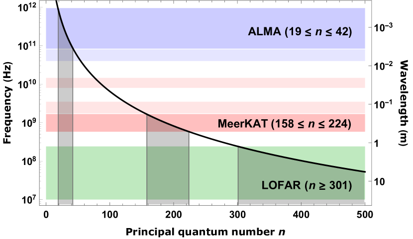
Figure 1: The black line shows the frequencies (wavelengths) of H$n\alpha$ transitions as a function of $n$ for hydrogen. The horizontal shaded bands depict the operating frequency bands of ALMA (blue), MeerKAT (red) and LOFAR (green). The lighter shaded bands are planned additions to the telescopes, but are not operational yet. The vertical grey shaded areas indicate the ranges of principal quantum number for which the H$n\alpha$ transitions will technically fall into the observing frequencies of the respective telescopes. A colour version of this graph is available in the electronic copy of this article.

Goldberg (1966) showed that at low frequencies where stimulated processes are important the accuracy of the calculation of atomic level populations has a substantial influence on the theoretical intensities of recombination lines. This sentiment is echoed 50 years later by Sánchez Contreras et al. (2017) who also point out that there is disagreement between the results of various authors without one set of values clearly being the correct one. The need for accurate values is even more important now that radio telescopes with high sensitivity are being constructed.

Burgess & Summers (1976) included stimulated emission and absorption terms for the bound-bound and bound-free transitions in an $n$-model that went up to principal quantum number $n=500$. They found that stimulated processes can have a significant effect on the values of the departure coefficients. This work was expanded by Summers (1977) who resolved the angular momentum states for levels with $n\leq 35$, but only considered how the ¹S, ²S and ²P levels of hydrogen were affected by a stellar radiation field. Brocklehurst & Salem (1977) and Salem & Brocklehurst (1979) published their programme and tables based on the $n$-model of Brocklehurst (1970) that gave departure coefficients for $50\leq n\leq 300$. The programme included updated collisional cross sections from Gee et al. (1976), collisions due to protons, as well as radiative processes involving an external field, but did not consider angular momentum changing collisions. The programme was modified by Walmsley (1990) to generate results down to $n=20$.

The results of Storey & Hummer (1995) (hereafter SH95) are considered to be the definitive values for optical/IR recombination lines, but stimulated processes are not included in their model. However, the values of SH95 are being used to study low frequency lines (see for example Fujiyoshi et al., 2006; Bendo et al., 2017; Sánchez Contreras et al., 2017). In this paper we present results using a model that includes stimulated and absorption processes in the bound-bound and bound-free transitions in an $nl$-model, and use updated numerical methods. Our results are compared to those of SH95. The current calculated values differ significantly from their results for levels with principal quantum number $n\gtrsim 30$.

In section 2 we describe our model and calculational details. A stopping criterion for an iterative method of solution is derived in section 3, and the results of including this in our calculations are compared with those of SH95. The use of a direct solver is also discussed here. The stimulating effects of continuum radiation fields within a nebula are considered in section 4. Finally, the main conclusions of this article are outlined in section 7. Details of the atomic calculations used in our model are presented in the appendix.

2 The model

To determine theoretical line intensities, the electron populations $N_{nl}$ of all bound states need to be calculated. The level populations $N_{nl}$ are described by statistical equilibrium which requires that the total rate of all transitions into any particular level must equal the total rate of the transitions out of that level.

Menzel (1937) introduced a correction factor, denoted by $b_{nl}$, to compensate for the degree of departure from local thermodynamic equilibrium (LTE) of the level population from the LTE value $N_{nl}^{*}$ so that

$$b_{nl}=\frac{N_{nl}}{N_{nl}^{*}}\,.$$ (1)

A departure coefficient $b_{nl}$ that is equal to unity indicates that the level $nl$ is in LTE with the electron gas. In this scheme, the Saha-Boltzmann equation for hydrogen becomes

$$N_{nl}=b_{nl}N_{\mathrm{e}}N_{\mathrm{p}}\left(\frac{h^{2}}{2\pi m_{\mathrm{e}}k_{\mathrm{B}}T_{\mathrm{e}}}\right)^{3/2}(2l+1)\exp\left(\frac{\chi_{nl}}{k_{\mathrm{B}}T_{\mathrm{e}}}\right)\,,$$ (2)

where $N_{\mathrm{e}}$ and $N_{\mathrm{p}}$ are the number density of electrons and protons respectively, $h$ is Planck’s constant, $m_{\mathrm{e}}$ is the electron mass, $k_{\mathrm{B}}$ is the Boltzmann constant and $T_{\mathrm{e}}$ is the kinetic temperature of the free electron gas. The ionisation potential of level $nl$ for hydrogen is given by $\chi_{nl}=R_{\mathrm{H}}hc/n^{2}$ where $R_{\mathrm{H}}$ is the Rydberg constant for hydrogen and $c$ the speed of light in a vacuum.

Collisional processes within the plasma become more efficient than their radiative counterparts as the principal quantum number $n$ of the level increases. Therefore, for each set of physical conditions there will be an $n=n^{*}$ where the collisional processes dominate completely and set up Boltzmann distributions with temperature $T_{\mathrm{e}}$ among the levels so that $b_{nl}=1$ for $n\geq n^{*}.$

Goldberg (1966) introduced an amplification factor $\beta_{n,n^{\prime}}$ with $n>n^{\prime}$ that is given by

$$\beta_{n,n^{\prime}}=\frac{\left(1-\frac{b_{n^{\prime}}}{b_{n}}e^{-h\nu/k_{\mathrm{B}}T_{\mathrm{e}}}\right)}{\left(1-e^{-h\nu/k_{\mathrm{B}}T_{\mathrm{e}}}\right)}$$ (3)

where $\nu$, the frequency associated with the $n$-$n^{\prime}$ transition, is given by

$$\nu=R_{\mathrm{H}}c\left(\frac{1}{n^{{}^{\prime}2}}-\frac{1}{n^{2}}\right)\,.$$ (4)

The amplification factors give the departure of the ratios of level populations from what is expected in LTE, as opposed to the departure coefficients that represent the departure of individual level populations from LTE. A value of $\beta_{n,n^{\prime}}<0$ indicates a population inversion between levels $n$ and $n^{\prime}$, with an increased amount of inversion for smaller values of $\beta_{n,n^{\prime}}$. Therefore, stimulated emission will be important for levels for which $\beta_{n,n^{\prime}}\ll 0$. An illustrative discussion of the amplification factor can be found in Strelnitski et al. (1996).

Baker & Menzel (1938) introduced two simple assumptions which are referred to as Case A and Case B. For Case A, the nebula is taken to be optically thin to all line radiation. For Case B, it is assumed that all photons produced by Lyman transitions are optically thick and are absorbed close to the point where they are emitted (this is called the on-the-spot approximation). From a calculational perspective, this means that all transitions to the $n=1$ level are ignored. Osterbrock (1962) concluded that Case B is a good quantitative approximation for nebular conditions.

Substituting the Saha-Boltzmann equation (2) into the rate equation of all processes due to statistical balance yields

$$\left(\frac{h^{2}}{2\pi m_{\mathrm{e}}k_{\mathrm{B}}T_{\mathrm{e}}}\right)^{-3/2}\left(\alpha_{nl}^{\mathrm{r}}+\alpha_{nl}^{\mathrm{s}}+N_{\mathrm{e}}C_{i,nl}\right)\ +$$

$$\underset{m>n}{\sum}\;\underset{l^{\prime}=l\pm 1}{\sum}b_{ml^{\prime}}(2l^{\prime}+1)e^{\chi_{ml^{\prime}}/k_{\mathrm{B}}T_{\mathrm{e}}}\left(A_{ml^{\prime},\,nl}+B_{ml^{\prime},\,nl}J_{\nu}+N_{\mathrm{e}}C_{ml^{\prime},\,nl}\right)$$

$$+\underset{k<n}{\sum}\;\underset{l^{{}^{\prime\prime}}=l\pm 1}{\sum}b_{kl^{{}^{\prime\prime}}}(2l^{{}^{\prime\prime}}+1)e^{\chi_{kl^{{}^{\prime\prime}}}/k_{\mathrm{B}}T_{\mathrm{e}}}\left(B_{kl^{{}^{\prime\prime}},\,nl}J_{\nu}+N_{\mathrm{e}}C_{kl^{{}^{\prime\prime}},\,nl}\right)$$

$$+\underset{l^{\prime}=l\pm 1}{\sum}b_{nl^{\prime}}(2l^{\prime}+1)e^{\chi_{nl^{\prime}}/k_{\mathrm{B}}T_{\mathrm{e}}}\sum_{q}N_{q}C^{q}_{nl^{\prime},\,nl}$$

$$=\ b_{nl}(2l+1)e^{\chi_{nl}/k_{\mathrm{B}}T_{\mathrm{e}}}\left[\alpha_{nl}^{\mathrm{p}}+N_{\mathrm{e}}C_{nl,i}\right.$$

$$\left.+\underset{k<n}{\sum}\;\underset{l^{{}^{\prime\prime}}=l\pm 1}{\sum}\left(A_{nl,\,kl^{{}^{\prime\prime}}}+B_{nl,\,kl^{{}^{\prime\prime}}}J_{\nu}+N_{\mathrm{e}}C_{nl\,kl^{{}^{\prime\prime}}}\right)\right.$$

$$\left.+\underset{m>n}{\sum}\;\underset{l^{\prime}=l\pm 1}{\sum}\left(B_{nl,\,ml^{\prime}}J_{\nu}+N_{\mathrm{e}}C_{nl,\,ml^{\prime}}\right)\ +\underset{l^{\prime}=l\pm 1}{\sum}\sum_{q}N_{q}C^{q}_{nl,\,nl^{\prime}}\right]\,.$$ (5)

The left-hand side contains all processes that populate level $nl$. The terms represent radiative recombination ($\alpha_{nl}^{\mathrm{r}}$), stimulated recombination ($\alpha_{nl}^{\mathrm{s}}$), three-body recombination ($C_{i,nl}$), spontaneous emission ($A_{nl,\,n^{\prime}l^{\prime}}$), stimulated emission ($B_{nl,\,n^{\prime}l^{\prime}}$), collisional de-excitation ($C_{nl,\,n^{\prime}l^{\prime}}$), absorption ($B_{n^{\prime}l^{\prime},\,nl}$), collisional excitation ($C_{n^{\prime}l^{\prime},\,nl}$) and elastic collisions ($C^{q}_{nl,\,nl^{\prime}}$). The mean intensity of incident radiation fields is given by $J_{\nu}$.

The right-hand side includes all processes that depopulate level $nl$. The terms represent photoionisation ($\alpha_{nl}^{\mathrm{p}}$), collisional ionisation ($C_{nl,i}$), spontaneous emission, stimulated emission, collisional de-excitation, collisional excitation, absorption and elastic collisions, respectively.

The $N_{q}$ represent the number densities of the different species interacting via elastic collisions with the bound electrons. In this work, electrons, protons and He⁺ ions are taken to induce these collisions, with the proton number density $N_{\mathrm{p}}=0.909N_{\mathrm{e}}$ and the He⁺ number density $N_{\mathrm{He}^{+}}=0.090N_{\mathrm{e}}$. These are the same values used by SH95.

Equation (5) represents a system of linear equations in the $b_{nl}$ values. Therefore, it can be written in matrix form as

$$\textbf{{A}}\mathbf{\cdot}\mathbf{b}=\mathbf{y}$$ (6)

where $\mathbf{b}$ is a vector with the $b_{nl}$ values as entries. The diagonal entries of the matrix A represent the processes depopulating a level $nl$ and the off-diagonal entries in a given row are the bound-bound processes that are populating that level. Only dipole transitions are considered in this work which results in A being sparse, i.e. most of the entries in the A matrix are equal to zero. The vector $\mathbf{y}$ contains the first term of equation (5) as well as the populating contributions of levels with $n>n_{\mathrm{c}}$.

The values of the $b_{nl}$’s for a specific set of conditions are found in a two step process. First, a set of equations for which the angular momentum states are not resolved are solved to obtain values for $b_{n}$. The values produced by this method are valid for $n>n_{\mathrm{c}}$ where the equation (7) holds. This is referred to as the $n$-model.

Next, equations (5) are solved explicitly for $n\leq n_{\mathrm{c}}$ to obtain the $b_{nl}$ values for this range. This part is referred to as the $nl$-model and the $b_{n}$’s for this range are obtained via equations (8). Sections 2.1 and 2.2 provide details regarding the the two parts of the model and calculational details of the individual rates in equation (5) are given in Appendix A.

2.1 The $n$-model

The approach of Brocklehurst (1970) was followed for the $n$-model. In addition to the processes in the Brocklehurst model, our $n$-model includes stimulated emission and absorption terms. In principle, an isolated atom has an infinite number of energy levels. To make the mathematics computationally viable, an upper cut-off $n_{\text{max}}$ was introduced for the highest $n$ level for which the rate equations were solved explicitly. The contributions to the sums above $n_{\text{max}}$ were converted into an integral using the trapezoidal rule. This integral was then approximated using a 20-point Gaussian quadrature. The remaining rate equations were cast into matrix form.

Because the departure coefficients vary smoothly and slowly with $n$, the Lagrange interpolation technique of Burgess & Summers (1969) was employed to reduce the number of equations to be solved five fold. The condensed rate equations were solved by direct Gaussian elimination with the use of partial pivoting. The resulting condensed vector containing the $b_{n}$ values was interpolated to give the full set of values. The $b_{n}$ values found using this method compared very well with the results of solving the full system of equations.

2.2 The $nl$-model

To obtain the departure coefficients for $n\leq n_{\mathrm{c}}$, the rate equations (5) have to be solved simultaneously. The main difference between the $b_{n}$’s from the $n$-model and the ones obtained from the $nl$-model and equation (8) is the inclusion of the elastic collisions between bound electrons and free particles. The elastic collisions’ effects are important for the populations of mid- to high-energy levels where the $b_{n}$’s calculated with the $nl$-model can differ significantly from those of the $n$-model.

The semi-classical impact-parameter formulation developed by Pengelly & Seaton (1964) for the rates of angular momentum changing collisions has been considered definitive for many decades. Recently, Vrinceanu et al. (2012) presented updated formulae for these transition rates for both the quantum and semi-classical case. Guzmán et al. (2016) did an in-depth analysis of the two approaches and concluded that the analytic equations presented in Pengelly & Seaton (1964) are much faster to compute and agree very well with the exact quantum mechanical probabilities of Vrinceanu et al. (2012). This supports an earlier conclusion of Storey & Sochi (2015). In this work, the formalism of Pengelly & Seaton (1964) was followed with the modification of Guzmán et al. (2016) to get the partial rates directly. Details are given in section A.2.2.

There will be a $n=n_{\mathrm{c}}<n^{*}$ where the collisional processes will be much faster than the radiative processes, but radiative effects are still evident. For $n_{\mathrm{c}}<n<n^{*}$, the angular momentum states are populated statistically according to

$$N_{nl}=\frac{2l+1}{n^{2}}N_{n}\,.$$ (7)

The departure coefficient, $b_{n}$, that represents the departure from LTE for an energy level $n$ is defined as the weighted sum of the $b_{nl}$’s

$$b_{n}=\frac{1}{n^{2}}\sum_{l=0}^{n-1}(2l+1)b_{nl}\,.$$ (8)

Therefore, it follows that $b_{n}=b_{nl}$ for $n>n_{\mathrm{c}}$.

Equation (5) represents a total of $n_{\mathrm{c}}(n_{\mathrm{c}}+1)/2$ equations that have to be solved simultaneously. This value is generally ${\sim}10^{4}$.

The populating contributions of the first $20$ energy levels beyond $n_{\mathrm{c}}$ are calculated explicitly and incorporated into the vector $\mathbf{y}$ in equation (6). The populating effects of levels $n>n_{\mathrm{c}}+20$ are approximated with a 20-point Gaussian quadrature in the same way as the contributions of $n>n_{\text{max}}$ are handled in the $n$-model and added to $\mathbf{y}$. The depopulating effects of levels with $n_{\mathrm{c}}<n\leq n_{\mathrm{c}}+20$ and $n>n_{\mathrm{c}}+20$ are treated similarly, but added to the total depopulation rate for each level contained in the diagonal of the matrix A.

The level $n_{\mathrm{c}}$ is determined empirically to ensure the results of the $nl$-model are used up to a sufficiently high principal quantum number so that they match the results of the $n$-model to four significant digits. The level above which equation (8) is valid was found to be weakly dependent on temperature and is calculated using

$$n_{\mathrm{c}}=350-15\ln(N_{\mathrm{e}})$$ (9)

and rounding up to the nearest multiple of $5$.

3 Stopping criterion

3.1 Background

Because the values of $b_{nl}$ do not vary smoothly, the matrix condensation technique used in the $n$-model cannot be employed at this step. The standard method of solving the large number of simultaneous equations in the $nl$-model is to use an iterative method (e.g. Brocklehurst, 1971; Smits, 1991; Storey & Hummer, 1995; Salgado et al., 2017). An important aspect of an iterative solution is a test to indicate when convergence of the departure coefficients has been achieved, and to stop the iterations. In most previous work, the stopping criterion has not been explicitly stated, except for Salgado et al. (2017), who terminate their iterative procedure when the difference between two successive iterations is less than 1 per cent.

We show here that such a stopping criterion is not appropriate and can stop the iterative process before the values of the departure coefficients have converged to values within a known error. If the iterative procedure is making small corrections to the $b_{nl}$’s, the convergence rate can be slow, with the result that a stopping criterion such as the one used by Salgado et al. (2017) can signal convergence has occured. Many more iterations can be required before convergence is reached. These tiny corrections can accumulate to a significant number, as will be shown below. For the conditions considered in this work, the matrix A has a condtion number $\kappa(\textbf{{A}})\sim 10^{7}$ which is very large and means the matrix is ill-conditioned, which results in a slow convergence rate (Douglas et al., 2016).

3.2 Derivation

To derive a stopping criterion, we define the following quantities and notation. Let $\mathbf{b}^{(i)}$ be the vector containing the departure coefficients as entries after $i$ iterations. The residual $\mathbf{r}^{(i)}$ after $i$ iterations is given by

$$\mathbf{r}^{(i)}=\textbf{{A}}\mathbf{\cdot}\mathbf{b}^{(i)}-\mathbf{y}$$ (10)

and provides an indication of the quality of $\mathbf{b}^{(i)}$. The vector of errors $\mathbf{e}^{(i)}$ after $i$ iterations is the difference between $\mathbf{b}^{(i)}$ and the true solution $\mathbf{b}$, i.e.

$$\mathbf{e}^{(i)}=\mathbf{b}^{(i)}-\mathbf{b}\,.$$ (11)

Of course, $\mathbf{b}$ is generally unknown and therefore $\mathbf{e}^{(i)}$ cannot be calculated directly. However, if an upper bound for the error can be defined then a stopping criterion can be constructed such that the iterations will only stop after it is guaranteed that the errors are smaller than some predefined number.

A norm of a vector or matrix, indicated using double bars $\|\cdot\|$, is a non-negative number that gives a measure of the magnitude of the vector or matrix. There are various types of norms that can be defined, all of which obey a specified set of properties. In particular, for a matrix M and vector $\mathbf{v}$ the inequality

$$\|\textbf{{M}}\mathbf{v}\|\leq\|\textbf{{M}}\|\|\mathbf{v}\|$$ (12)

will hold for any consistent pair of vector and matrix norms. Note that the quantity called the condition number mentioned above is defined as

$$\kappa(\textbf{{M}})=\|\textbf{{M}}^{-1}\|\ \|\textbf{{M}}\|\,.$$ (13)

If $\kappa(\textbf{{M}})\gg 1$ then the matrix is called ill-conditioned.

Using the tools developed above, an appropriate stopping criterion for an iterative solution to the set of equations represented by equation (6) can now be derived. Substituting equation (6) into equation (11) and using equation (10) gives

$$\mathbf{e}^{(i)} =\mathbf{b}^{(i)}-\textbf{{A}}^{-1}\mathbf{y}$$

$$=\textbf{{A}}^{-1}(\textbf{{A}}\mathbf{\cdot}\mathbf{b}^{(i)}-\mathbf{y})$$

$$=\textbf{{A}}^{-1}\mathbf{r}^{(i)}.$$ (14)

Taking the norm on both sides and using the submultiplicative property given in equation (12) leads to

$$\|\mathbf{e}^{(i)}\|=\|\textbf{{A}}^{-1}\mathbf{r}^{(i)}\|\leq\|\textbf{{A}}^{-1}\|\|\mathbf{r}^{(i)}\|\,.$$ (15)

Therefore, stopping the iterative procedure only after

$$\|\mathbf{r}^{(i)}\|\leq\epsilon\mathbf{\cdot}\frac{\|\mathbf{b}^{(i)}\|}{\|\textbf{{A}}^{-1}\|}$$ (16)

will guarantee that the relative error is smaller than some predefined tolerance $\epsilon\ll 1$. That is, equation (16) implies

$$\frac{\|\mathbf{e}^{(i)}\|}{\|\mathbf{b}^{(i)}\|}\leq\frac{\|\textbf{{A}}^{-1}\|\|\mathbf{r}^{(i)}\|}{\|\mathbf{b}^{(i)}\|}\leq\epsilon\,.$$ (17)

Equation (17) is true for any consistent pair of vector and submultiplicative matrix norms.

One appropriate set of such norms is the $l_{1}$ norm of a vector and the corresponding operator norm of a matrix. For a general $n$-vector $\mathbf{v}$ with components $v_{i}$ and a general $n\times n$ matrix M with entries $m_{ij}$, these norms are given respectively by

$$\|\mathbf{v}\|_{1}=\sum_{i=1}^{n}|v_{i}|\qquad\mathrm{and}\qquad\|\textbf{{M}}\|_{1}=\max_{1\leq j\leq n}\sum_{i=1}^{n}\left|m_{ij}\right|\,.$$ (18)

The matrix norm $\|\textbf{{M}}\|_{1}$ corresponds to the maximum sum of the absolute values of the individual columns of M.

Calculating matrix inverses are notoriously expensive. Because an algorithm for estimating the $l_{1}$ norm of the inverse of a matrix is available, these norms have been used. The algorithm of Hager (1984) that estimates the $l_{1}$ norm of the inverse of a matrix without inverting the matrix first, was refined by Higham (1988). This algorithm usually gives the exact value of $\|\textbf{{A}}^{-1}\|_{1}$ and, at worst, gives an order of magnitude estimate for the types of matrices considered here (Higham, 1988). The values of $\|\mathbf{b}^{(i)}\|_{1}$ and $\|\mathbf{r}^{(i)}\|_{1}$ can be calculated directly.

3.3 Effects on departure coefficients

In this section an iterative procedure is applied to the linear system (5) in order to show the effect of the stopping criterion given in equation (16) on the departure coefficients. The procedure is a derivative of the Gauss-Seidel method and is described in Brocklehurst (1971). The same method was used by SH95 and Salgado et al. (2017).

The results of the $n$-model are refined using this iterative scheme as follows. The departure coefficients $b_{n}$ from the $n$-model are used as the initial values so that $b_{nl}=b_{n}$ at the start of the algorithm. The rate equation (5) is then solved to obtain $b_{nl}$ for decreasing values of $n$ starting with $n=n_{\mathrm{c}}$. The $b_{nl}$ values for a given $n$ are solved simultaneously as an $n\times n$ matrix by including all the terms that do not depend on these specific $b_{nl}$ values in the right-hand side of equation (6). Each newly calculated set of $b_{nl}$’s is used in subsequent calculations down to $n=2$ for Case A and $n=3$ for Case B. This constitutes one iteration and the process is repeated until the stopping criterion (16) is met.

Fig. 2 shows the evolution of a subset of departure coefficients as the iterative procedure progresses for a gas at $T_{\mathrm{e}}=10^{4}$ K with density $N_{\mathrm{e}}=10^{4}$ cm^-3 for Case B with no external radiation field present. The values on the left-hand side of the graph show the values after one iteration and the values on the far right indicate the values after convergence is reached. For this case, the $b_{nl}$’s converged to four significant digits ($\epsilon=5\times 10^{-5}$) after $1\,375$ iterations. The dashed vertical line at 3 iterations indicates the first point in the process where the departure coefficients from two successive iterations change by less than 1 per cent. From the graph it is clear that a small change in the departure coefficients during the procedure is not sufficient to indicate convergence.

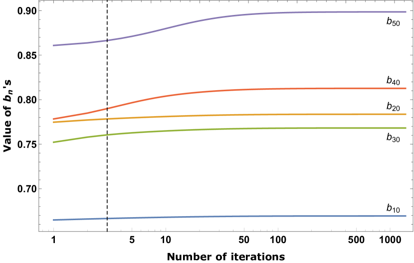
Figure 2: The evolution of five departure coefficients for $T_{\mathrm{e}}=10^{4}$ K, $N_{\mathrm{e}}=10^{4}$ cm^-3 Case B as the iterative procedure of the $nl$-model progresses. Convergence is reached after 1 375 iterations. The dashed line at 3 iterations shows the first point where the values of the $b_{nl}$’s change by less than 1 per cent.

4 Comparison to previous results

A comparison of the current results with those of SH95 for a range of temperatures at a fixed electron density of $N_{\mathrm{e}}=10^{4}$ cm^-3 is shown in Fig. 3. The largest discrepancy occurs at intermediate principal quantum numbers. This is unsurprising, since the behaviour of the $b_{nl}$’s at low and high $n$’s are not governed by the $nl$-model. At low energy levels, radiative processes dominate and the departure coefficients would be largely unaffected by the elastic collisions introduced in the $nl$-model. Therefore, at these levels the final $b_{nl}$’s will be very close to their initial values obtained from the $n$-model. At high energy levels, the collisional processes dominate completely and all $b_{nl}$’s will tend towards unity, reducing the difference between the two sets of calculations.

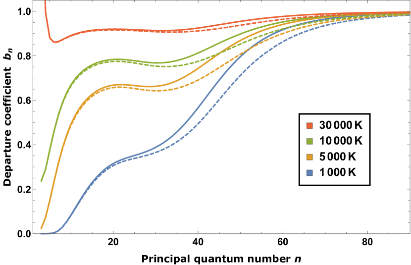
Figure 3: Departure coefficients $b_{n}$ for Case B for a variety of temperatures at electron density $N_{\mathrm{e}}=10^{4}$ cm^-3. Dashed lines represent the values obtained by SH95 and solid lines in the same colour show the current results for the same conditions. A colour version of this figure is available in the electronic version of the article.

Fig. 4 shows the difference between the unsummed $b_{nl}$ values of SH95 and the current work. As expected, the differences are very small for low values of $n$, but become more pronounced as $n$ and $l$ increase. This effect is due to elastic collisions becoming the dominant process at intermediate and high $n$ levels.

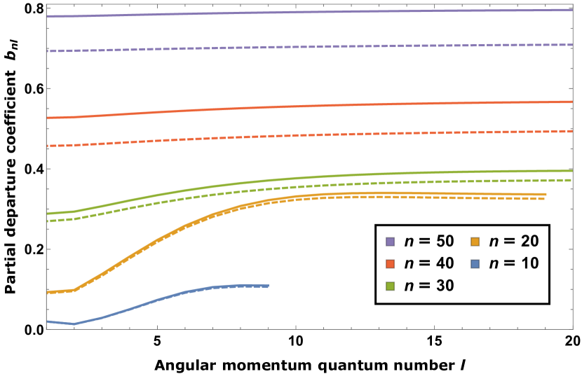
Figure 4: Partial departure coefficients $b_{nl}$ for a selected number of principal quantum numbers $n$ for $T_{\mathrm{e}}=10^{3}$ K and $N_{\mathrm{e}}=10^{4}$ cm^-3, Case B. Solid lines represent the calculations of this work, dashed lines of the same colour show the results of SH95 for the same $n$. A colour version of this figure is available in the electronic version of the article.

The results show that line enhancement by stimulated emission of H$n\alpha$ transitions for intermediate $n$ are less extreme than previously thought, with the point of maximum inversion occurring at a lower level. Fig. 5 illustrates the amplification factor as defined in equation (3) for H$n\alpha$ transitions for the same parameters as Fig. 3. The lines that fall in the optical range are largely unaffected, with the largest deviation from previous results in the radio regime.

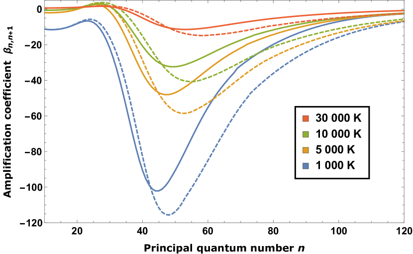
Figure 5: The amplification factor $\beta_{n,n+1}$ for H$n\alpha$ transitions for electron density $N_{\mathrm{e}}=10^{4}$ cm^-3 and a range of temperatures under Case B conditions. Solid lines show the current results and dashed lines are those of SH95. A colour version of this figure is available in the electronic version of the article.

The discrepancy between our values and those of SH95 increases as the temperature decreases and the density increases; there is a stronger dependence on temperature than density. For $T_{\mathrm{e}}=500$ K and $N_{\mathrm{e}}=10^{6}$ cm^-3 the maximum relative difference is 22.5 per cent. We can match the values of SH95 within a per cent by terminating our procedure prematurely. Storey (private communication) has noted that the SH95 model converges extremely fast (within 10 iterations) and that the departure coefficients do not change significantly if either the number of iterations or $n_{c}$ is increased.

At this stage we do not understand the reasons that the SH95 model converges so fast and to different values than ours. The differences in inelastic collisional rates between the models certainly plays a role, but does not account fully for the differences. We have performed many tests on our model, but cannot get it to converge as fast or to the same values as SH95. Clearly, this is an issue that will need further investigation.

Obtaining a solution from thousands of iteration steps takes a significant amount of time. To speed up the solution, a direct solver using the PARDISO package (Petra et al., 2014a; Petra et al., 2014b) was tested. It is a sophisticated solver for systems of linear equations that exploits the sparsity of A to solve the system in a very efficient manner. The direct solver is considerably faster at solving the set of linear equations than the iterative method.

The departure coefficients shown in the rest of the paper were obtained using the above direct solver package. The $b_{nl}$’s obtained from the iterative method with the given stopping criterion match those using the direct solver. An error estimate of the quality of the results of the direct solver was obtained using

$$\epsilon\approx\|\textbf{{A}}\cdot\mathbf{b}-\mathbf{y}\|/\|\mathbf{b}\|\,.$$ (19)

It was found that $\epsilon\leq 10^{-4}$ in all cases.

5 Stimulating effects of continuum radiation

In this section we examine the effects of the continuum radiation fields on the population structure of hydrogen in nebular environments. Specifically, their role in stimulating transitions between electronic states.

The continuum radiation in the diffuse ISM consists of different components, each of which are examined to determine their effect on departure coefficients. The radiation fields considered here are the stellar radiation field, the free-free radiation field generated by the electrons in the gas, the cosmic microwave background radiation (CMBR) and emission from dust.

Fig. 6 shows the mean intensity $J_{\nu}$ of these fields as a function of the frequency associated with H$n\alpha$ transitions. The population inversion of the excited electrons is most pronounced for energy levels $30\lesssim n\lesssim 80$ (refer to Fig. 5), so that electrons in these levels are susceptible to being stimulated.

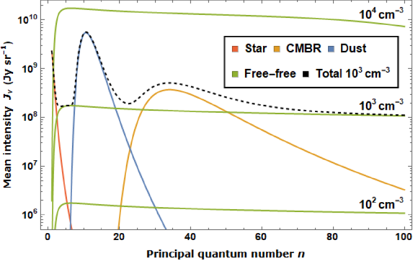
Figure 6: Spectrum of continuum radiation fields $J_{\nu}$ within a model ionised nebula at $T_{\mathrm{e}}=10^{4}$ K. The free-free field is shown for three different densities. The horizontal axis shows the principal quantum number for H$n\alpha$ transitions, and the vertical axis shows the mean intensities of the various radiation fields.

5.1 Stellar radiation field

Photoionised nebulae require a nearby hot source of ultraviolet radiation to ionise atoms in the gas. In Fig. 6 the blackbody radiation field from a $T=50\,000$ K source with dilution factor $W=10^{-12}$ is shown on the far left. As can be seen, the intensity of the ionising radiation from such a hot star drops off very quickly with decreasing frequency (increasing $n$ in the diagram) and is negligible at frequencies low enough to stimulate transitions in hydrogen. An O or B star has to be a distance of $\lesssim 10\,\mathrm{AU}$ from the gas to have any noticeable effect on the departure coefficients and, therefore, can be neglected in these calculations.

5.2 Cosmic microwave background radiation

The CMBR has a low temperature ($T=2.7$ K) but is undiluted blackbody radiation. Coincidentally, the intensity of the radiation peaks around a frequency corresponding to H$n\alpha$ with $n\sim 40$ which is where the population inversion is strongest.

For a density of $N_{\mathrm{e}}=10^{2}$ cm^-3 stimulated emissions due to the CMBR make up in excess of 10 per cent of the downward $\mathrm{H}n\alpha$ transitions for $40\lesssim n\lesssim 60$. As the density increases, the effect of stimulated emission decreases because the influence of elastic collisions increase at these levels. The correction that the inclusion of the CMBR in the model provides to the summed $b_{nl}$’s is typically less than 1 per cent.

5.3 Free-free radiation

Continuous free-free radiation is produced by a plasma as charged free particles interact with each other without capture taking place. The free particles are assumed to be in thermodynamic equilibrium at a temperature $T_{\mathrm{e}}$. Disregarding background radiation, the specific intensity of the free-free radiation is given by

$$J_{\nu}^{\mathrm{ff}}=B_{\nu}(T_{\mathrm{e}})\left(1-e^{-\tau_{\nu}^{\mathrm{ff}}}\right)\,,$$ (20)

where $B_{\nu}$ is the Planck function for frequency, and $\tau_{\nu}^{\mathrm{ff}}$ is the optical depth of this radiation.

Following Dickinson et al. (2003), the appropriate optical depth for the free-free radiation is given by

$$\tau_{\nu}^{\mathrm{ff}} =-3.014\times 10^{-2}\,T_{\mathrm{e}}^{-3/2}\left(\frac{10^{9}}{\nu}\right)^{2}$$

$$\times\left[\ln\left(4.955\times 10^{-2}\nu^{-1}\right)+1.5\ln\left(T_{\mathrm{e}}\right)\right](\mathrm{EM})\,,$$ (21)

where EM is the emission measure in cm^-6 pc. For a homogeneous gas, EM = $N_{\mathrm{e}}^{2}$ cm^-6 pc.

The intensity of the free-free radiation within a nebula is strongly dependent on the electron density $N_{\mathrm{e}}$. The effect of this radiation on the population structure of hydrogen is negligible for low densities, but can become significant for $N_{\mathrm{e}}>10^{4}$ cm^-3. For example, the departure coefficients of a gas with $N_{\mathrm{e}}=10^{6}$ cm^-3 and $T_{\mathrm{e}}=10^{4}$ K will be affected by up to 12 per cent around $n=20$ by the inclusion of the free-free radiation field due to stimulated processes, as illustrated in Fig. 7. The free-free radiation affects departure coefficients for principal quantum numbers in the range $10\lesssim n\lesssim 60$.

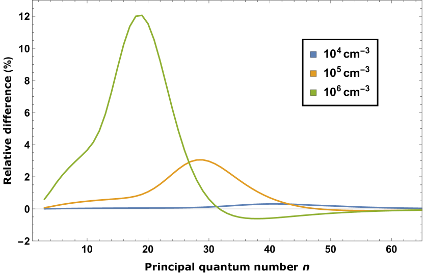
Figure 7: The effects of the free-free radiation field on the population structure of hydrogen for $T_{\mathrm{e}}=10^{4}$ K, and a range of densities in Case B. The relative difference between the departure coefficients calculated when no radiation field is present and when the free-free field is included in the calculations are shown for each principal quantum number.

5.4 Dust

Dust grains form an important component of the ISM and have been found to be intermixed with the ionised media of H ii regions and planetary nebulae (Barlow, 1993; Kingdon & Ferland, 1997). Emission from dust grains can dominate the spectrum from H ii regions and PNe at long wavelengths, outshining the free-free specific intensity by orders of magnitudes.

To model the emission from dust within the cloud, a modified blackbody spectrum of the form

$$J_{\nu}^{\mathrm{d}}=\tau_{\nu}^{\mathrm{d}}B_{\nu}(T_{\mathrm{d}})\,,$$ (22)

was used, where $\tau_{\nu}^{\mathrm{d}}$ is an optical depth and $T_{\mathrm{d}}$ is the dust temperature (Planck Collaboration et al., 2014). The angle-averaged optical depth

$$\tau_{\lambda}^{\mathrm{d}}=1.5\times 10^{-3}\left(\frac{100\mathrm{\mu m}}{\lambda}\right)^{1.7}$$ (23)

from Draine (2011) was used.

The effect of the dust radiation on the $b_{n}$ values is very limited as the populations are only weakly inverted at the frequencies where this radiation can stimulate transitions. In Fig. 6 a dust temperature of $T_{\mathrm{d}}=50$ K (Dupac et al., 2003) is shown, but the result is independent of $T_{\mathrm{d}}$ since this has little effect on the frequency range of the field.

In this work we have only considered the effect of the radiation from dust on the level populations. Hummer & Storey (1992) have shown that absorption by dust can affect the Case B recombination spectrum, possibly with a greater effect on the departure coefficients than emission.

6 Description of tables

The programme described here calculates departure coefficients $b_{nl}$ for level $nl$ in hydrogen. From this, theoretical spectral line intensities can be calculated. The formulae required to calculate values that can be compared with observed lines are presented below, and then the entries in the tables are explained.

NE = 10000 TE = 10000 CASE B NC = 210 NO RAD
-------------------------------------------------------------------
BN’S
3	2.374e-01	4	2.895e-01	5	3.769e-01	6	4.616e-01	7	5.328e-01	8	5.897e-01	9	6.344e-01	10	6.694e-01	11	6.968e-01	12	7.184e-01
13	7.355e-01	14	7.489e-01	15	7.595e-01	16	7.678e-01	17	7.741e-01	18	7.787e-01	19	7.818e-01	20	7.836e-01	21	7.842e-01	22	7.838e-01
$\boldsymbol{\vdots}$
BNL’S
n = 3
0	1.022e+00	1	2.336e-01	2	8.271e-02
n = 4
0	1.132e+00	1	3.300e-01	2	1.446e-01	3	2.553e-01
n = 5
0	1.206e+00	1	3.973e-01	2	1.891e-01	3	3.235e-01	4	4.239e-01
$\boldsymbol{\vdots}$
JNM’S
n = 4
1	1.217e-25	2	9.879e-27	3	3.289e-27
n = 5
1	5.304e-26	2	4.633e-27	3	1.602e-27	4	7.710e-28
n = 6
1	2.830e-26	2	2.563e-27	3	8.903e-28	4	4.426e-28	5	2.432e-28
$\boldsymbol{\vdots}$
KMN’S
n = 4
3	3.271e-23
n = 5
3	1.003e-23	4	-8.418e-25
n = 6
3	4.463e-24	4	2.892e-24	5	-1.518e-23
$\boldsymbol{\vdots}$

Table 1: An extract of one of the output tables for the conditions $T_{\mathrm{e}}=10^{4}$ K and $N_{\mathrm{e}}=10^{4}$ cm^-3, Case B, with no external radiation present. The values of the departure coefficients ($b_{n}$), the partial departure coefficients ($b_{nl}$), the emission coefficients ($j_{nn^{\prime}}$) and the absorption coefficients ($\kappa_{n^{\prime}n}$) are tabulated for each case.

The emission coefficient $j_{nn^{\prime}}$ for line radiation is given by

$$j_{nn^{\prime}}=\frac{h\nu}{4\pi}\sum_{l=0}^{n-1}\sum_{l^{\prime}=l\pm 1}b_{nl}N_{nl}^{*}A_{nl,n^{\prime}l^{\prime}}$$ (24)

and the absorption coefficient by

$$\kappa_{n^{\prime}n}=\frac{h\nu}{4\pi}\sum_{l=0}^{n-1}\sum_{l^{\prime}=l\pm 1}\left[b_{nl}N_{nl}^{*}B_{n^{\prime}l^{\prime},nl}\left(1-\frac{b_{nl}}{b_{n^{\prime}l^{\prime}}}e^{-h\nu/k_{\mathrm{B}}T_{\mathrm{e}}}\right)\right]\,.$$ (25)

The tables containing our results are available online in machine-readable ASCII format and can be downloaded from the article webpage. The file names are a concatenation of the significands and exponents of the electron density and temperature, the case (A or B) and any ambient radiation that has been included in the model, all separated by an underscore. Free-free radiation is indicated by ‘FF’, the CMBR by ‘CMB’, and no radiation field is designated with the number ‘0’. For example, the file named ‘13_14_B_0.dat’ contains the results for Case B with $N_{\mathrm{e}}=10^{4}$ cm^-3 and $T_{\mathrm{e}}=10^{4}$ K with no ambient radiation present. The header in each file contains the same data as in the file name, as well as the value of $n_{\mathrm{c}}$.

Each file contains the $b_{n}$ values calculated using equation (8) for each value of $n$ from $n=2$ for Case A and $n=3$ for Case B to $n=500$. This is followed by the partial departure coefficients $b_{nl}$ with the appropriate values of $l$ tabulated after each value of $n$ up to $n=100$. The emission coefficients $j_{nn^{\prime}}$ and absorption coefficients $\kappa_{n^{\prime}n}$ as defined by equations (24) and (25), respectively, are given next. The coefficients are tabulated next to the lower level $n^{\prime}$ for ascending values of the upper level $n$. An extract of one of the data files is shown in table 1.

7 Conclusions

Updated calculations of departure coefficients for hydrogen atoms under nebular conditions are presented. The elastic collision rates of Guzmán et al. (2016) have been used, which differ from values used in previous models. We have also included stimulated and absorption processes in our equations of statistical equilibrium. The model used to do the calculations is similar to that of SH95.

A stopping criterion has been derived and employed to determine when to terminate the iterative procedure, which ensures that the $b_{nl}$ values have converged to a predefined accuracy. This requires that many more iterative steps are required before a solution is reached than have been used in previous works. In practice, we found that it is more time efficient to use a direct solver rather than the iterative method to achieve an acceptable accuracy.

We investigated the effects of stimulated emission due to various components of the continuum field within a nebula on the population structure of hydrogen. Even though the stellar radiation field and emission from dust dominate the continuum spectrum at certain frequencies, the effects on the population structure of both fields are negligible. The free-free radiation field has the largest influence on the departure coefficients, increasing as the density increases. The CMBR typically has an effect of less than 1 per cent on the departure coefficients.

Our results give departure coefficients that are consistently larger (closer to LTE) than those of SH95. The current results produce amplification factors $\beta_{n,n+1}$ that are smaller than in previous calculations, producing less extreme population inversions. The value of $n_{\mathrm{c}}$, the level at which populations become statistically distributed, has been determined empirically. The value, which depends on the electron density $N_{\mathrm{e}}$, is much larger than used in other models.

Results for He and metal atoms and ions will be considered in a separate publication.

Appendix A Calculational details

The various atomic rates used in our calculations are based on standard algorithms from the literature which, in many cases, have been used by numerous authors over the years. There are possibly slight differences in formulae used for large values of $n$ and the values at which these approximations are used, and therefore, for completeness, we present in this section how we calculated the various rates. Because there is as yet no compelling evidence to indicate that particles in astronomical plasmas obey anything other than regular thermodynamic velocity distributions, all our velocity distribution functions are Maxwellian.

Although the $n$-method models are run before the $nl$-models, we usually calculate the $nl$-model atomic rates first, and then use these with the appropriate weighting to determine the $n$-model value. The conversion formulae we used are presented at the end of each section.

The symbols used are: $a_{0}$ is the Bohr radius, $c$ is the speed of light in a vacuum, $e$ is the elementary charge, $g_{nl}$ is the statistical weight of level $nl$, $h$ is Planck’s constant, $k_{\mathrm{B}}$ is Boltzmann’s constant, $m_{\mathrm{e}}$ is the electron mass, $R_{\mathrm{H}}$ is the Rydberg constant for hydrogen, $T_{\mathrm{e}}$ is the kinetic temperature of the free electron gas, $Z$ is the atomic charge, $\alpha$ is the fine structure constant, and $\nu$ is the frequency of the emitted or absorbed photon.

A.1 Radiative processes

Because electric dipole transitions are orders of magnitude larger than forbidden transitions, only transitions that satisfy $l\rightarrow l\pm 1$ are included in our models.

A.1.1 Bound-bound transitions

The rate of a spontaneous dipole transition from level $nl$ to a lower energy level $n^{\prime}l^{\prime}$ is calculated using (Brocklehurst, 1971)

$$A_{nl,\,n^{\prime}l^{\prime}}=\frac{64\pi^{4}\nu^{3}}{3Z^{2}hc^{3}}\frac{\max(l,\,l^{\prime})}{2l+1}e^{2}a_{0}^{2}\left[\tau_{nl}^{n^{\prime}l^{\prime}}\right]^{2}$$ (26)

in cgs units, where $\tau_{nl}^{n^{\prime}l^{\prime}}$ is the bound-bound radial dipole matrix element of the transition. An explicit formula for the bound-bound dipole matrix element of a transition between $nl$ and $n^{\prime}\,l-1$ for hydrogen is given by Gordon (1929). The matrix element $\tau_{nl}^{n^{\prime}\,l+1}$ for a transition $nl\rightarrow n^{\prime}\,l+1$ is obtained by making the substitutions $n\rightarrow n^{\prime}$ and $l\rightarrow l+1$ in the above formula.

Direct calculation of the matrix elements $\tau_{nl}^{n^{\prime}l^{\prime}}$ is impractical for large principal quantum numbers due to overflow errors in the calculation of the hypergeometric functions. An iterative scheme described by van Regemorter et al. (1979) is used to calculate $\tau_{nl}^{n^{\prime}l^{\prime}}$ for large $n$. The results were compared to the tables of Green et al. (1957), which are almost identical to the relativistic transition probabilities of Wiese & Fuhr (2009), and show good agreement.

The Einstein A-values for the $n$-model, $A_{nn^{\prime}}$, are obtained from (26) using

$$A_{nn^{\prime}}=\frac{1}{n^{2}}\sum_{l}\sum_{l^{\prime}=l\pm 1}\left(2l+1\right)A_{nl,\,n^{\prime}l^{\prime}}\,.$$ (27)

For levels with $n>500$, the approximation due to Menzel (1937) for the A-value is used, which is given by

$$A_{nn^{\prime}}=\frac{16\alpha^{4}c}{3\pi\sqrt{3}a_{0}}\frac{g_{nn^{\prime}}}{n^{3}n^{\prime}(n^{2}-n^{\prime 2})}$$ (28)

where $g_{nn^{\prime}}$ is the bound-bound Gaunt factor that is approximated by

$$g_{nn^{\prime}}=1-\frac{0.1728\left(1+n^{\prime 2}/n^{2}\right)}{\left(1-n^{\prime 2}/n^{2}\right)^{2/3}\left(n^{\prime}\right)^{2/3}}\,.$$ (29)

For high $n$-levels, the approximation (28) generally performs well. Because collisional processes will always dominate over radiative processes at these levels (for the conditions considered here), inaccuracies introduced by this approximation are not important.

The rate coefficients for stimulated emission $B_{nl,\,n^{\prime}l^{\prime}}$ and absorption $B_{n^{\prime}l^{\prime},\,nl}$ are calculated using the Einstein relations (Einstein, 1916) given by

$$B_{nl,\,n^{\prime}l^{\prime}}=\frac{g_{n^{\prime}l^{\prime}}}{g_{nl}}B_{n^{\prime}l^{\prime},\,nl}=\frac{c^{2}}{2h\nu^{3}}A_{nl,\,n^{\prime}l^{\prime}}\,.$$ (30)

A.1.2 Bound-free transitions

Radiative recombination

The radiative recombination rate coefficient $\alpha_{nl}^{\mathrm{r}}$ to the level $nl$ is defined by

$$N_{\mathrm{e}}N_{\mathrm{p}}\alpha_{nl}^{\mathrm{r}}=N_{\mathrm{e}}N_{\mathrm{p}}\int\sigma_{nl}^{r}(v)\,vf(v)\,dv$$ (31)

where $\sigma_{nl}^{\mathrm{r}}(v)$ is the radiative recombination cross-section and $f(v)$ is the speed distribution of the free electrons.

An expression for $\alpha_{nl}^{\mathrm{r}}$ that uses a Maxwellian distribution with a temperature $T_{\mathrm{e}}$ for the free electron velocities is given by Burgess (1965) as

$$\alpha_{nl}^{\mathrm{r}}=\left(\frac{2\pi^{1/2}\alpha^{4}a_{0}^{2}c}{3}\right)\frac{2y^{1/2}}{n^{2}}\sum_{l^{\prime}=l\pm 1}I\!\left(n,\,l,\,l^{\prime},\,T_{\mathrm{e}}\right)$$ (32)

where

$$I\!\left(n,\,l,\,l^{\prime},\,T_{\mathrm{e}}\right) =\mathrm{max}\!\left(l,\,l^{\prime}\right)\,y$$

$$\times\intop_{0}^{\infty}\left(1+n^{2}\kappa^{2}\right)^{2}\Theta\!\left(n,\,l;\,\kappa,\,l^{\prime}\right)\mathrm{e}^{-y\kappa^{2}}\;d\!\left(\kappa^{2}\right)$$ (33)

and

$$y=\frac{R_{\mathrm{H}}hc}{k_{\mathrm{B}}T_{\mathrm{e}}},\qquad\Theta(n,\,l;\,\kappa,\,l^{\prime})=\left(1+n^{2}\kappa^{2}\right)\left|\tau_{nl}^{\kappa l^{\prime}}\right|^{2}\,.$$ (34)

The parameter $\kappa$ is the energy of the free electron expressed in terms of the ionisation energy of hydrogen so that the energy difference between the bound and free states is given by

$$h\nu=\left(1+n^{2}\kappa^{2}\right)\chi_{n}$$ (35)

with $\chi_{n}=\chi_{1}/n^{2}$ the ionisation energy of level $n$.

The radial dipole matrix elements for transitions between a bound and a free state $\tau_{nl}^{\kappa l^{\prime}}$ are computed using the recurrence relations given by Burgess (1965). These equations satisfy the exact matrix elements for hydrogenic atoms. Burgess (1965) observes that severe scaling problems can occur with this method for large $n$. This was overcome by doing calculations with the natural logarithm of the recurrence relations. The natural logarithm reduces the size of the numbers stored in the computer memory at intermediate steps, thereby preventing overflow errors.

The integration in (33) is performed with a Gaussian integration technique. The integrands vary very rapidly when $\kappa$ is small, and much slower for large $\kappa$. Following Burgess (1965), a number of five-point Gaussian integrations are made, starting with an interval size of $h=10^{-4}n^{-1}$. The interval size was doubled after every five-point integration and the procedure is terminated when the sum of the integrals is accurate up to six significant digits.

The total radiative recombination coefficient into an energy level $n$ is given by the sum of the partial coefficients over the angular momentum states so that

$$\alpha_{n}^{\mathrm{r}}=\sum_{l=0}^{n-1}\alpha_{nl}^{\mathrm{r}}\,.$$ (36)

Photoionisation

The rate coefficient for photoionisation $\alpha_{nl}^{\mathrm{p}}(\nu)$ for the level $nl$ is given by

$$N_{nl}\alpha_{nl}^{\mathrm{p}}=N_{nl}\int_{\chi_{nl}/h}^{\infty}a_{nl}^{\mathrm{p}}(\nu)\frac{4\pi J_{\nu}}{h\nu}\,d\nu\,.$$ (37)

where $J_{\nu}$ is the mean intensity of the ambient radiation field and $a_{nl}^{\mathrm{p}}(\nu)$ is the photoionisation cross section from level $nl$ for a photon with frequency $\nu$.

The photoionisation cross-section to level $nl$ for a hydrogenic atom is calculated using the formula of Burgess (1965), which is given by

$$a_{nl}^{\mathrm{p}}\!\left(\kappa^{2}\right)=\left(\frac{4\pi\alpha a_{0}^{2}}{3}\right)n^{2}\sum_{l^{\prime}=l\pm 1}\frac{\max(l,\,l^{\prime})}{2l+1}\,\Theta\!\left(n,\,l;\,\kappa,\,l^{\prime}\right)\,.$$ (38)

Putting equation (38) into (37) and using equation (35), the photoionisation coefficient $\alpha_{nl}^{\mathrm{p}}$ can be written as

$$\alpha_{nl}^{\mathrm{p}} =\left(\frac{4\pi R_{\mathrm{H}}c\alpha a_{0}^{2}}{3}\right)\frac{n^{2}}{2l+1}\int_{0}^{\infty}\left(\frac{4\pi J_{\nu}}{h\nu}\right)_{\kappa^{2}}$$

$$\times\sum_{l^{\prime}=l\pm 1}\max(l,\,l^{\prime})\,\Theta\!\left(n,\,l;\,\kappa,\,l^{\prime}\right)\,d\left(\kappa^{2}\right)\,.$$ (39)

The subscript $\kappa^{2}$ indicates that the quantity inside the brackets should be written in terms of $\kappa^{2}$ before integration. The integral in (39) is handled in the same manner as for radiative recombination.

The total photoionisation coefficient for hydrogen from level $n$ is given by

$$\alpha_{n}^{\mathrm{p}}=\sum_{l=0}^{n-1}\frac{2l+1}{n^{2}}\alpha_{nl}^{\mathrm{p}}\,.$$ (40)

Stimulated recombination

The cross-section for stimulated recombination $\sigma_{nl}^{\mathrm{s}}(v)$ of an electron with a speed $v$ into level $nl$ is related to the photoionisation cross-section $a_{nl}^{\mathrm{p}}$ (see equation (38)) by

$$\sigma_{nl}^{s}=\frac{g_{nl}}{8\pi g_{i}}\frac{h^{2}}{m_{\mathrm{e}}^{2}v^{2}}a_{nl}^{\mathrm{p}}\,.$$ (41)

The rate of stimulated recombination in the presence of a radiation field $J_{\nu}$ with a free electron velocity distribution $f(v)$ is given by

$$\alpha_{nl}^{\mathrm{s}}=\int_{\chi_{nl}/h}^{\infty}\frac{4\pi J_{\nu}}{h\nu}\sigma_{nl}^{\mathrm{s}}(v)\,f(v)\frac{h}{m_{\mathrm{e}}}\,d\nu\,.$$ (42)

Putting equation (38) into (41) gives the stimulated recombination cross-section, and in turn putting the result into equation (42) gives the stimulated recombination coefficient as

$$\alpha_{nl}^{\mathrm{s}} =\left(\frac{4\pi R_{\mathrm{H}}c\alpha a_{0}^{2}}{3}\right)\left(\frac{m_{\mathrm{e}}}{2\pi k_{B}T_{\mathrm{e}}}\right)^{3/2}\left(\frac{h}{m_{\mathrm{e}}}\right)^{3}n^{2}$$

$$\times\int_{0}^{\infty}\left(\frac{4\pi J_{\nu}}{h\nu}\right)_{\kappa^{2}}\sum_{l^{\prime}=l\pm 1}\max(l,\,l^{\prime})\,\Theta\!\left(n,\,l;\,\kappa,\,l^{\prime}\right)e^{-y\kappa^{2}}d(\kappa^{2})$$ (43)

The integration is evaluated numerically using a Gaussian quadrature scheme as described above for radiative recombination.

The total stimulated recombination coefficient to an energy level $n$ of hydrogen is given by

$$\alpha_{n}^{\mathrm{s}}=\sum_{l=0}^{n-1}\alpha_{nl}^{\mathrm{s}}\,.$$ (44)

A.2 Collisional transitions

A.2.1 Inelastic collisions

The semi-empirical formulae of Vriens & Smeets (1980) are used to calculate the rates for collisional de-excitation $C_{n,n^{\prime}}$ between the bound states $n$ and $n^{\prime}$. These values are valid over a wider range of temperatures than the values obtained from the formulae of Gee et al. (1976) which were used by SH95. Vriens & Smeets (1980) claim that their results agree within 5 to 20 per cent with those of Gee et al. (1976) in the regimes where both calculations are valid.

SH95 resolved the collision rates between angular momentum states using

$$C_{nl,\,n^{\prime}l^{\prime}}=\frac{A_{nl,\,n^{\prime}l^{\prime}}}{A_{nn^{\prime}}}C_{nn^{\prime}}$$ (45)

for $\Delta l=\pm 1$, which is based on the Coulomb-Bethe approximation. SH95 used this approximation for transitions with $n^{\prime}=n\pm 1$ and

$$C_{nl,\,n^{\prime}l^{\prime}}=C_{nn^{\prime}}\quad\mbox{for}\quad n^{\prime}\neq n\pm 1\,.$$ (46)

In our calculations the approximation in equation (45) is used throughout; detailed balance is used to calculate the rates of the inverse process. We included interactions between all levels with $n\neq n^{\prime}$. Because elastic collision rates are higher than inelastic collision rates for all $n$ for which collisions are important, $l$-levels are populated predominantly by angular momentum-changing collisions, and, hence, the exact dependence of the inelastic collision rates on angular momentum is not that important.

We use the rates of collisional ionisation $C_{n,i}$ from the formulae of Vriens & Smeets (1980). The assumption $C_{nl,i}=C_{n,i}$ is used in the $nl$-model, since this process is never significant at the conditions considered here. The three-body recombination rates $C_{i,n}$ and $C_{i,nl}$ are obtained from detailed balance considerations. Vriens & Smeets (1980) found that their formulae for the bound-free collisional rates agreed with experimental data to within 10 to 30 per cent.

A.2.2 Elastic collisions

Brocklehurst (1971) used an iterative scheme to calculate the partial rate coefficients $C_{nl,nl\pm 1}$ based on the work of Pengelly & Seaton (1964). Hummer & Storey (1987) pointed out that this method caused oscillatory behaviour in the rate coefficients as a function of $l$. They avoided this by normalizing the collision cross-sections with the oscillator strengths of the transitions.

In this work, the formalism of Pengelly & Seaton (1964) is followed based on the recommendation of Storey & Sochi (2015) and Guzmán et al. (2016). The modification suggested by Guzmán et al. (2016) to get the partial rates directly is utilized. The relevant equations in cgs units are

$$C_{nl,nl} =9.93\times 10^{-6}\sqrt{\frac{\mu}{m}}\frac{D_{nl,nl^{\prime}}}{\sqrt{T_{\mathrm{e}}}}N_{\mathrm{e}}$$

$$\times\left[11.54+\log_{10}\left(\frac{mT_{\mathrm{e}}}{\mu D_{nl,nl}}\right)+2\log_{10}\left(R_{\mathrm{c}}\right)\right]$$ (47)

with

$$D_{nl,nl^{\prime}}=\left(\frac{Z_{\mathrm{p}}}{Z_{\mathrm{t}}}\right)^{2}\frac{6n^{2}\max(l,\,l^{\prime})\left[n^{2}-\max(l,\,l^{\prime})^{2}\right]}{2l+1}$$ (48)

where $m$ and $Z_{\mathrm{p}}$ are the mass and charge of the projectile particle, $Z_{\mathrm{t}}$ is the charge of the target atom or ion, $\mu$ is the reduced mass of the colliding system, and $R_{\mathrm{c}}$ is the effective cut-off radius of the interaction at large impact parameters as given by Pengelly & Seaton (1964).

In practice, $C_{nl,nl+1}$ is calculated using (47) and $C_{nl,nl-1}$ is obtained using the principle of detailed balance

$$C_{nl,\,nl^{\prime}}=\frac{2l^{\prime}+1}{2l+1}C_{nl^{\prime},\,nl}\,.$$ (49)

References

- Anantharamaiah (2002) Anantharamaiah K. R., 2002, in Pramesh Rao A., Swarup G., Gopal-Krishna eds, IAU Symposium Vol. 199, The Universe at Low Radio Frequencies. p. 319
- Baker & Menzel (1938) Baker J. G., Menzel D. H., 1938, ApJ, 88, 52
- Barlow (1993) Barlow M. J., 1993, in Weinberger R., Acker A., eds, IAU Symposium Vol. 155, Planetary Nebulae. p. 163
- Bendo et al. (2017) Bendo G. J., Miura R. E., Espada D., Nakanishi K., Beswick R. J., D’Cruze M. J., Dickinson C., Fuller G. A., 2017, MNRAS, 472, 1239
- Brocklehurst (1970) Brocklehurst M., 1970, MNRAS, 148, 417
- Brocklehurst (1971) Brocklehurst M., 1971, MNRAS, 153, 471
- Brocklehurst & Salem (1977) Brocklehurst M., Salem M., 1977, Computer Physics Communications, 13, 39
- Burgess (1965) Burgess A., 1965, MmRAS, 69, 1
- Burgess & Summers (1969) Burgess A., Summers H. P., 1969, ApJ, 157, 1007
- Burgess & Summers (1976) Burgess A., Summers H. P., 1976, MNRAS, 174, 345
- Dickinson et al. (2003) Dickinson C., Davies R. D., Davis R. J., 2003, MNRAS, 341, 369
- Douglas et al. (2016) Douglas C. C., Lee L., Yeung M.-C., 2016, Procedia Computer Science, 80, 941
- Draine (2011) Draine B. T., 2011, Physics of the Interstellar and Intergalactic Medium. Princeton University Press
- Dupac et al. (2003) Dupac X., et al., 2003, A&A, 404, L11
- Einstein (1916) Einstein A., 1916, Deutsche Physikalische Gesellschaft, 18, 318
- Fujiyoshi et al. (2006) Fujiyoshi T., Smith C. H., Caswell J. L., Moore T. J. T., Lumsden S. L., Aitken D. K., Roche P. F., 2006, MNRAS, 368, 1843
- Gee et al. (1976) Gee C. S., Percival L. C., Lodge J. G., Richards D., 1976, MNRAS, 175, 209
- Goldberg (1966) Goldberg L., 1966, ApJ, 144, 1225
- Gordon (1929) Gordon W., 1929, Annalen der Physik, 394, 1031
- Green et al. (1957) Green L. C., Rush P. P., Chandler C. D., 1957, apjs, 3, 37
- Guzmán et al. (2016) Guzmán F., Badnell N. R., Williams R. J. R., van Hoof P. A. M., Chatzikos M., Ferland G. J., 2016, MNRAS, 459, 3498
- Hager (1984) Hager W. W., 1984, SIAM Journal on Scientific and Statistical Computing, 5, 311
- Higham (1988) Higham N. J., 1988, ACM Transactions on Mathematical Software (TOMS), 14, 381
- Hummer & Storey (1987) Hummer D. G., Storey P. J., 1987, MNRAS, 224, 801
- Hummer & Storey (1992) Hummer D. G., Storey P. J., 1992, MNRAS, 254, 277
- Kingdon & Ferland (1997) Kingdon J. B., Ferland G. J., 1997, ApJ, 477, 732
- Menzel (1937) Menzel D. H., 1937, ApJ, 85, 330
- Osterbrock (1962) Osterbrock D. E., 1962, ApJ, 135, 195
- Pengelly & Seaton (1964) Pengelly R. M., Seaton M. J., 1964, MNRAS, 127, 165
- Petra et al. (2014a) Petra C. G., Schenk O., Anitescu M., 2014a, IEEE Computing in Science & Engineering, 16, 32
- Petra et al. (2014b) Petra C. G., Schenk O., Lubin M., Gärtner K., 2014b, SIAM Journal on Scientific Computing, 36, C139
- Planck Collaboration et al. (2014) Planck Collaboration et al., 2014, A&A, 571, A11
- Salem & Brocklehurst (1979) Salem M., Brocklehurst M., 1979, ApJS, 39, 633
- Salgado et al. (2017) Salgado F., Morabito L. K., Oonk J. B. R., Salas P., Toribio M. C., Röttgering H. J. A., Tielens A. G. G. M., 2017, ApJ, 837, 141
- Sánchez Contreras et al. (2017) Sánchez Contreras C., Báez-Rubio A., Alcolea J., Bujarrabal V., Martín-Pintado J., 2017, A&A, 603, A67
- Smits (1991) Smits D. P., 1991, MNRAS, 248, 193
- Storey & Hummer (1995) Storey P. J., Hummer D. G., 1995, MNRAS, 272, 41
- Storey & Sochi (2015) Storey P. J., Sochi T., 2015, MNRAS, 446, 1864
- Strelnitski et al. (1996) Strelnitski V. S., Ponomarev V. O., Smith H. A., 1996, ApJ, 470, 1118
- Summers (1977) Summers H. P., 1977, MNRAS, 178, 101
- Vriens & Smeets (1980) Vriens L., Smeets A. H. M., 1980, PhRvA, 22, 940
- Vrinceanu et al. (2012) Vrinceanu D., Onofrio R., Sadeghpour H. R., 2012, ApJ, 747, 56
- Walmsley (1990) Walmsley C. M., 1990, A&AS, 82, 201
- Wiese & Fuhr (2009) Wiese W. L., Fuhr J. R., 2009, J. Phys. Chem. Ref. Data, 38, 565
- van Regemorter et al. (1979) van Regemorter H., Binh Dy H., Prudhomme M., 1979, Journal of Physics B Atomic Molecular Physics, 12, 1053