Back-Reaction of Gravitational Waves Revisited

Abstract

We study the back-reaction of gravitational waves in early universe cosmology, focusing both on super-Hubble and sub-Hubble modes. Sub-Hubble modes lead to an effective energy density which scales as radiation. Hence, the relative contribution of such gravitational waves to the total energy density is constrained by big bang nucleosynthesis. This leads to an upper bound on the tensor spectral slope $n_{T}$ which also depends on the tensor to scalar ratio $r$. Super-Hubble modes, on the other hand, lead to a negative contribution to the effective energy density, and to an equation of state of curvature. Demanding that the early universe is not dominated by the back-reaction leads to constraints on the gravitational wave spectral parameters which are derived.

I Introduction

Gravitational waves (GW) carry energy and momentum and hence affect the background space-time they propagate in. This is a basic consequence of the nonlinearity of the Einstein field equations. The effects of gravitational waves propagating on a given space-time on the space-time itself is called gravitational back-reaction.

A spectrum of primordial gravitational waves is generated Starob in early universe scenarios such as inflationary cosmology infl , but also BNPV2 in alternatives such as string gas cosmology BV ; SGrev . The spectrum is characterized by its amplitude ${\cal A}_{T}$ and spectral tilt $n_{T}$. If $k_{*}$ is the comoving wavenumber used as the pivot scale (e.g. the scale of the quadrupole of the cosmic microwave background (CMB)), then the power spectrum of gravitational waves on scale $k$ is given by

$${\cal P}_{T}(k)\,=\,A_{T}(k_{*})\left(\frac{k}{k_{*}}\right)^{n_{T}}\,.$$ (1)

The amplitude of the gravitational wave spectrum at the pivot scale is related to the observed amplitude of the spectrum of cosmological perturbations on that scale via the tensor-to-scalar ratio $r_{*}$, with the subscript $*$ denoting that the amplitudes are evaluated at the pivot scale. The current upper bound on the value of $r_{*}$ is $0.07$ at 95 % C.L. BICEP . Even assuming that the amplitude of gravitational waves is close to the current upper bound, the current limits on the slope $n_{T}$ are weak Stewart . It is interesting to explore the possibility that gravitational back-reaction considerations can lead to improved constraints.

Short wavelength (wavelengths smaller than the Hubble radius) gravitational waves oscillate and have the same equation of state as radiation. Hence, Big Bang Nucleosynthesis sets an upper bound on the energy in short wavelength gravitational waves.

The effects of long wavelength (super-Hubble) waves is much less studied. It is sometimes claimed that causality prevents such modes from having a locally measurable effect (see, e.g., Wald ). This, however, is incorrect. First of all, in all models which yield a solution of the horizon problem of Standard Big Bang Cosmology, and in which a causal explanation of the origin of structure is possible, the cosmological horizon (the forward light cone of a point at the time when the initial conditions are imposed) is much larger than the Hubble radius. In the case of inflationary cosmology, the horizon at the end of the period of inflation has a radius which is larger by a factor of $e^{N}$ than the Hubble radius, where $N$ is the total number of $e$-foldings of inflation. Hence there is no causality argument which prohibits super-Hubble (but sub-horizon) modes from having a back-reaction effect (see e.g. Fabio1 for a discussion of this point). In fact, since super-Hubble gravitational waves give a non-vanishing contribution to the local effective energy-momentum tensor, they are able to have a local effect on the background geometry.

There has been more focus on the back-reaction effects of super-Hubble scalar cosmological perturbations (scalar fluctuations about a homogeneous and isotropic background). If we consider linearized cosmological fluctuations, then the effective energy-momentum tensor with which these fluctuations back-react on the background metric is quadratic in the amplitude of the fluctuations. In Abramo1 ; Abramo2 the form of this effective energy-momentum tensor was derived, and it was shown that the effective energy-momentum tensor of super-Hubble modes has the form of a negative cosmological constant. This follows from the fact that both spatial and temporal derivative terms in the effective energy-momentum tensor are suppressed on super-Hubble scales, leaving only terms which act like scalar field potential energy. Since on super-Hubble scales the negativity of the effective gravitational energy overwhelms the positivity of the matter energy, the contribution is like that of a negative cosmological constant. This gives rise to the possibility of a dynamical relaxation mechanism for the cosmological constant (see RHBbrReview for a review and Polyakov ; WT1 for similar ideas).

The effects of super-Hubble gravitational waves in a de Sitter universe (no matter present) has been considered in a series of papers by Tsamis and Woodard WT . They find that at two loop order, long wavelength modes induce a negative contribution to the cosmological constant and could thus lead to a relaxation of the bare cosmological constant. On the other hand, in Abramo2 it was shown that in a universe which contains matter and hence scalar metric perturbations, the super-Hubble modes have an equation of state (mode by mode)

$$p\,=\,-\frac{1}{3}\rho\,,$$ (2)

with $p$ and $\rho$ denoting pressure and energy densities, respectively. This is the equation of state of spatial curvature. As for scalar metric fluctuations, the sign of the effective energy density is negative.

As first pointed out by Unruh Unruh , the local observability of back-reaction effects of super-Hubble modes is an important issue. In fact, it was shown in Ghazal1 ; AW that for adiabatic cosmological perturbations the back-reaction effect of super-Hubble modes is equivalent to a second order time translation. On the other hand, in models with a separate clock field (like the radiation field in our current matter-dominated cosmology) the back-reaction effects of super-Hubble modes are locally measurable Ghazal2 , and they correspond to a decrease in the observed Hubble expansion rate Vacca . Locally, the back-reaction of infrared modes manifests itself in a change of the locally measured cosmological constant and curvature scalar Lam .

In a model which contains matter, the physical time $t$ which appears in the Friedmann-Robertson-Walker line element (see below) is related to the energy density of matter. Matter plays the role of a physical clock, and hence any effects on the local Hubble expansion rate which we find as a consequence of including long wavelength gravitational waves is a physical effect and not a gauge artefact.

In this paper we revisit the question of back-reaction effects of gravitational waves in a universe which is dominated by its matter content. We consider the back-reaction effects of the totality of the modes, both infrared (super-Hubble) and ultraviolet (sub-Hubble). We study not only a nearly de Sitter phase of expansion, but consider effects in the radiation and matter periods of Standard Big Bang cosmology, assuming a spectrum of gravitational waves produced in the early universe. We also study the dependence of our results on the tensor to scalar ratio $r$ and on the spectral index $n_{T}$.

What is new in our work concerning super-Hubble modes compared to previous works is that we compute the magnitude and equation of state of the totality of IR modes. We consider the three phases of the standard inflationary paradigm of cosmology, namely the de Sitter phase, the radiation phase and the final matter phase, and study the dependence of the results on the tensor to scalar ratio $r$ and on the tensor tilt $n_{T}$. Regarding sub-Hubble modes, we consider the dependence of the results on $r$ and $n_{T}$ and discuss constraints on $r$ and $n_{T}$ which can be derived.

A word on our notation. We use the signature $(-,+,+,+)$ for the metric. Physical time is denoted $t$, and $x$ are the spatial comoving coordinates. Greek letters are for space-time indices, Latin ones for space only indices. The scale factor is denoted $a(t)$, and the Hubble expansion rate by $H(t)$. It is often convenient to work in terms of conformal time $\tau$ related to the physics time $t$ via $dt=a(t)d\tau$. In conformal time, the Hubble expansion rate is denoted by ${\cal H}$. The derivative with respect to conformal time is indicated by a prime.

II Effective Energy-Momentum Tensor of Gravitational Waves

We will consider a background space-time given by a homogeneous and isotropic metric with scale factor $a(t)$. To this background we add scalar and tensor metric fluctuations of small amplitude which satisfy the linear fluctuation equations (see e.g. MFB for an overview of the theory of cosmological perturbations and RHBrev for a shorter introduction). Because of the nonlinearities in the Einstein field equations, the resulting metric fails to be a solution of the equations at second order. In order to have a solution of the Einstein equations at second order, we need to add second order terms in the metric. These include a correction to the background metric and corrections to the fluctuations. Both of these are of second order.

As described in Abramo1 ; Abramo2 , the correction to the background metric can be found by inserting the ansatz for the metric with only linear fluctuations into the Einstein equations, expanding to second order in the amplitude of the fluctuations, and then taking the spatial average of the resulting equations to extract the back-reaction effect on the background metric. Each Fourier mode of the fluctuations contributes independently to the back-reaction.

The spatial averaging also eliminates any coupling between scalar and tensor metric fluctuations at this order in perturbation theory. Hence, we can study the back-reaction of scalar and tensor modes separately. Here we will focus on the back-reaction of the tensor modes. Hence, we can set the scalar fluctuations to zero and consider the metric

$$ds^{2}\,=\,-a^{2}d\tau^{2}+a^{2}\left[\gamma_{ij}+h_{ij}\right]dx^{i}dx^{j}\,,$$ (3)

where $\gamma_{ij}$ is the spatial background metric, and $h_{ij}$ is the transverse and traceless tensor of linearized gravitational waves.

The Einstein tensor at second order can be written as

$$\delta^{(2)}G^{0}_{~{}0} = \frac{1}{a^{2}}\left[\mathcal{H}h^{km}h^{{}^{\prime}}_{km}+\frac{1}{8}h^{{}^{\prime}km}h^{{}^{\prime}}_{km}-\frac{1}{8}h^{{}^{\prime}k}_{~{}~{}k}h^{{}^{\prime}m}_{~{}~{}m}-\frac{1}{2}h^{km}\nabla^{2}h_{km}-\frac{1}{2}h^{km}h^{j}_{~{}~{}j,km}\right.$$ (4)

$$~{}~{}\left.+h^{km}h^{j}_{~{}~{}k,mj}-\frac{1}{4}h^{m~{}~{},k}_{~{}~{}m}h^{~{}~{},j}_{kj}+\frac{1}{8}h^{m~{}~{},k}_{~{}~{}m}h^{j}_{~{}j,k}-\frac{3}{8}h^{km,j}h_{km,j}\right.$$

$$~{}~{}\left.+\frac{1}{4}h^{km}_{~{}~{}~{}~{},k}\left(2h^{~{}~{}~{},j}_{mj}-h^{j}_{~{}j,m}\right)+\frac{1}{4}h^{jk,m}h_{jm,k}\right],$$

$$\delta^{(2)}G^{0}_{~{}i} = \frac{1}{a^{2}}\left[\frac{1}{2}h^{mk}_{~{}~{}~{}~{},m}h^{{}^{\prime}}_{ki}+h^{mk}h^{{}^{\prime}}_{k[i,m]}-\frac{1}{4}h^{{}^{\prime}mk}h_{mk,i}-\frac{1}{4}h^{k~{}~{},j}_{~{}~{}k}h^{{}^{\prime}}_{ij}\right],$$ (5)

$$\delta^{(2)}G^{i}_{~{}0} = \frac{1}{a^{2}}\left[h^{ij}h^{{}^{\prime}k}_{~{}~{}[k,j]}+\frac{1}{4}h^{k}_{~{}~{}k,j}h^{{}^{\prime}ij}-\frac{1}{2}h^{~{}~{}~{},j}_{jk}h^{{}^{\prime}ik}+\frac{1}{4}h^{{}^{\prime}}_{jk}h^{jk,i}-h_{jk}h^{{}^{\prime}k[i,j]}\right],$$

$$\delta^{(2)}G^{i}_{~{}j} = \frac{1}{a^{2}}\delta^{i}_{~{}j}\left[\mathcal{H}h^{{}^{\prime}}_{km}h^{km}+\frac{1}{2}h^{{}^{\prime\prime}}_{km}h^{km}+\frac{3}{8}h^{{}^{\prime}}_{km}h^{{}^{\prime}km}-\frac{1}{8}h^{{}^{\prime}k}_{~{}~{}~{}k}h^{{}^{\prime}m}_{~{}~{}~{}m}\right.$$ (7)

$$~{}~{}\left.-\frac{1}{2}h^{km}\left(\nabla^{2}h_{km}+h^{j}_{~{}j,km}-2h^{j}_{~{}(k,m)j}\right)-\frac{3}{8}h^{km,j}h_{km,j}\right.$$

$$~{}~{}\left.-\frac{1}{8}h^{m~{}~{},k}_{~{}~{}m}\left(2h^{,j}_{kj}-h^{j}_{~{}~{}j,k}\right)+\frac{1}{4}h^{km}_{~{}~{}~{}~{},k}\left(2h^{~{}~{}~{},j}_{mj}-h^{j}_{~{}~{}j,m}\right)+\frac{1}{4}h^{jk,m}h_{jm,k}\right]$$

$$+\frac{1}{a^{2}}\left[-\mathcal{H}h^{ik}h^{{}^{\prime}}_{kj}-\frac{1}{2}h^{ik}h^{{}^{\prime\prime}}_{kj}-\frac{1}{2}h^{{}^{\prime}ik}h^{{}^{\prime}}_{kj}+\frac{1}{4}h^{{}^{\prime}k}_{~{}~{}k}h^{{}^{\prime}i}_{~{}~{}j}+\frac{1}{4}h^{km,i}h_{km,j}\right.$$

$$~{}~{}\left.+\frac{1}{2}h^{ik}h^{m}_{~{}~{}m,kj}+\frac{1}{2}h^{m~{}~{},k}_{~{}~{}m}h^{(i}_{~{}~{}k,j)}-\frac{1}{4}h^{m~{}~{},k}_{~{}~{}m}h^{i}_{~{}~{}j,k}\right.$$

$$~{}~{}\left.+\frac{1}{2}h^{km}\left(h^{~{}~{}~{},i}_{km~{},j}+h^{i}_{~{}~{}j,km}-2h^{(i}_{~{}~{}m,j)k}\right)-\frac{1}{2}h^{km}_{~{}~{}~{},k}\left(2h^{~{}~{}(i}_{m~{}~{},j)}-h^{i}_{~{}~{}j,m}\right)\right.$$

$$~{}~{}\left.+h^{i[k,m]}h_{kj,m}-h^{ik}h^{m}_{~{}~{}(k,j)m}+\frac{1}{2}h^{ik}\nabla^{2}h_{kj}\right].$$

These expressions can be simplified by using the transverse and traceless condition $\partial^{i}h_{ij}=h^{i}_{~{}i}=0$ on the gravitational wave tensor. Then, the Einstein tensor simplifies to

$$\delta^{(2)}G^{0}_{~{}0} = \frac{1}{a^{2}}\left[\mathcal{H}h^{km}h^{{}^{\prime}}_{km}+\frac{1}{8}h^{{}^{\prime}km}h^{{}^{\prime}}_{km}+\frac{1}{8}h^{km,j}h_{km,j}-\frac{1}{2}\partial^{j}\left(h^{km}h_{km,j}\right)+\frac{1}{4}\partial_{k}\left(h^{jk,m}h_{jm}\right)\right],$$ (8)

$$\delta^{(2)}G^{0}_{~{}i} = \frac{1}{a^{2}}\left[h^{mk}h^{{}^{\prime}}_{k[i,m]}-\frac{1}{4}h^{{}^{\prime}mk}h_{mk,i}\right],$$ (9)

$$\delta^{(2)}G^{i}_{~{}0} = \frac{1}{a^{2}}\left[\frac{1}{4}h^{{}^{\prime}}_{jk}h^{jk,i}-h_{jk}h^{{}^{\prime}k[i,j]}\right],$$ (10)

$$\delta^{(2)}G^{i}_{~{}j} = \frac{1}{a^{2}}\delta^{i}_{~{}j}\left[\mathcal{H}h^{{}^{\prime}}_{km}h^{km}+\frac{1}{2}h^{{}^{\prime\prime}}_{km}h^{km}+\frac{3}{8}h^{{}^{\prime}}_{km}h^{{}^{\prime}km}\right.$$ (11)

$$~{}~{}\left.-\frac{1}{2}\partial_{j}\left(h^{km}h_{km}\right)+\frac{1}{2}h^{km,j}h_{km,j}-\frac{3}{8}h^{km,j}h_{km,j}+\frac{1}{4}\partial^{m}\left(h^{jk}h_{jm,k}\right)\right]$$

$$+\frac{1}{a^{2}}\left[-\mathcal{H}h^{ik}h^{{}^{\prime}}_{kj}-\frac{1}{2}h^{ik}h^{{}^{\prime\prime}}_{kj}-\frac{1}{2}h^{{}^{\prime}ik}h^{{}^{\prime}}_{kj}+\frac{1}{4}h^{km,i}h_{km,j}\right.$$

$$~{}~{}\left.+\frac{1}{2}\partial_{j}\left(h^{km}h^{~{}~{}~{},i}_{km~{}~{}}\right)-\frac{1}{2}h^{km}_{~{}~{}~{},j}h^{~{}~{}~{},i}_{km}+\frac{1}{2}\partial_{m}\left(h^{km}h^{i}_{~{}j,k}\right)\right.$$

$$~{}~{}\left.-\partial_{k}\left(h^{km}h^{~{}~{}(i}_{m~{}~{},j)}\right)-\frac{1}{2}\partial_{m}\left(h^{im,k}h_{kj}\right)+\frac{1}{2}\partial^{m}\left(h^{ik}h_{kj,m}\right)\right].$$

The spatial average of a quantity $A$ is obtained by integrating over the constant time hypersurface and dividing by the spatial volume $V$ Abramo2 :

$$\left\langle A\right\rangle\equiv\frac{1}{V}\lim_{V\rightarrow\infty}\int AdV.$$ (12)

Note that in the presence of matter, this hypersurface has a physical meaning: it is the surface of constant matter energy density.

Thus, denoting spatial averages by pointed parentheses, the spatially averaged Einstein tensors become

$$\left\langle\delta^{(2)}G^{0}_{~{}0}\right\rangle = \frac{1}{a^{2}}\left[\mathcal{H}\left\langle h^{km}h^{{}^{\prime}}_{km}\right\rangle+\frac{1}{8}\left\langle h^{{}^{\prime}km}h^{{}^{\prime}}_{km}\right\rangle+\frac{1}{8}\left\langle h^{km,j}h_{km,j}\right\rangle\right],$$ (13)

$$\left\langle\delta^{(2)}G^{0}_{~{}i}\right\rangle = \frac{1}{a^{2}}\left[\left\langle h^{mk}h^{{}^{\prime}}_{k[i,m]}\right\rangle-\frac{1}{4}\left\langle h^{{}^{\prime}mk}h_{mk,i}\right\rangle\right],$$ (14)

$$\left\langle\delta^{(2)}G^{i}_{~{}0}\right\rangle = \frac{1}{a^{2}}\left[\frac{1}{4}\left\langle h^{{}^{\prime}}_{jk}h^{jk,i}\right\rangle-\left\langle h_{jk}h^{{}^{\prime}k[i,j]}\right\rangle\right],$$ (15)

$$\left\langle\delta^{(2)}G^{i}_{~{}j}\right\rangle = \frac{1}{a^{2}}\delta^{i}_{~{}j}\left[\frac{3}{8}\left\langle h^{{}^{\prime}}_{km}h^{{}^{\prime}km}\right\rangle-\frac{3}{8}\left\langle h^{km,n}h_{km,n}\right\rangle\right]$$ (16)

$$+\frac{1}{a^{2}}\left[-\frac{1}{2}\left\langle h^{{}^{\prime}ik}h^{{}^{\prime}}_{kj}\right\rangle-\frac{1}{4}\left\langle h^{km,i}h_{km,j}\right\rangle+\frac{1}{2}\left\langle h^{ik,m}h_{kj,m}\right\rangle\right],$$

where the terms with a total derivative have been dropped since we are taking a spatial average. In addition, we have also used the equation of motion for $h_{ij}$:

$$h_{ij}^{{}^{\prime\prime}}+2\mathcal{H}h_{ij}^{\prime}-\nabla^{2}h_{ij}=0.$$ (17)

Taking the above correction terms to the Einstein tensor to the matter side of the cosmological equations, we can read off the effective energy density and effective pressure of gravitational waves. The energy density is

$$\rho_{\rm GW}=\frac{1}{8\pi G}\delta G^{0}_{~{}0}=\frac{1}{8\pi Ga^{2}}\left(\frac{1}{8}\left\langle(h^{\prime}_{ij})^{2}\right\rangle+\frac{1}{8}\left\langle(\nabla h_{ij})^{2}\right\rangle+\mathcal{H}\left\langle h^{ij}h{{}^{\prime}}_{ij}\right\rangle\right),$$ (18)

and the pressure is given by Abramo2

$$p_{\rm GW} = \frac{1}{3}\frac{1}{8\pi G}G^{i}_{~{}i}+\frac{1}{3{\cal H}}\left\langle{}^{(2)}\Gamma^{\alpha}_{~{}\alpha 0}\right\rangle(\rho^{(0)}+p^{(0)})$$ (19)

$$= \frac{1}{3}\frac{1}{8\pi Ga^{2}}\left(-\frac{5}{8}\left\langle(h^{\prime}_{ij})^{2}\right\rangle+\frac{7}{8}\left\langle(\nabla h_{ij})^{2}\right\rangle\right)-\frac{1}{3{\cal H}}\left\langle{}^{(2)}\Gamma^{\alpha}_{~{}\alpha 0}\right\rangle(\rho^{(0)}+p^{(0)})$$

$$= \frac{1}{3}\frac{1}{8\pi Ga^{2}}\left(-\frac{5}{8}\left\langle(h^{\prime}_{ij})^{2}\right\rangle+\frac{7}{8}\left\langle(\nabla h_{ij})^{2}\right\rangle\right)+\frac{1}{2}\frac{1}{8\pi Ga^{2}}{\cal H}\left(1+w^{(0)}\right)\left\langle h^{ij}h^{\prime}_{ij}\right\rangle\,.$$

Here $w^{(0)}$ is the equation of state parameter for the cosmological background (i.e., $\rho^{(0)}+p^{(0)}=\rho^{(0)}(1+w^{(0)})$). In the last equality, we have used the fact that

$$\left\langle{}^{(2)}\Gamma^{\alpha}_{~{}\alpha 0}\right\rangle=-\frac{1}{2}\left\langle h^{ij}h^{\prime}_{ij}\right\rangle,$$ (20)

and the Friedmann equation

$$H^{2}=\frac{{\cal H}^{2}}{a^{2}}=\frac{8\pi G}{3}\rho^{(0)}.$$ (21)

Now we work in Fourier space. One can expand $h_{ij}(\tau,{\bm{x}})$ as follows:

$$h_{ij}(\tau,{\bm{x}})=\sum_{\lambda=+,\times}\int\frac{dk^{3}}{(2\pi)^{3}}\epsilon_{ij}^{\lambda}({\bm{k}})h_{\bm{k}}^{\lambda}(\tau)e^{i{\bm{k}}\cdot{\bm{x}}},$$ (22)

where $\epsilon_{ij}^{\lambda}$ is the polarization tensor which is symmetric in $i$ and $j$. It also satisfies the transverse-traceless condition and the normalization condition

$$\sum_{i,j}\left\langle\epsilon_{ij}^{\lambda}({\bm{k}})\epsilon_{ij}^{\lambda^{\prime}}({\bm{k}^{\prime}})\right\rangle\,=\,2\delta^{\lambda\lambda^{\prime}}\delta^{(3)}({\bm{k}}-{\bm{k}}^{\prime}).$$ (23)

In Fourier space, the equation of motion for the gravitational waves is

$$h^{{}^{\prime\prime}}_{\bm{k}}+2{\cal H}h^{{}^{\prime}}_{\bm{k}}+k^{2}h_{\bm{k}}=0.$$ (24)

By substituting the expansion given in Eq. (22), the energy density and pressure of gravitational waves can be written as

$$\rho_{\rm GW}^{\rm(tot)} = \frac{1}{8\pi Ga^{2}}\sum_{\lambda}\int\frac{dk}{k}\frac{k^{3}}{\pi^{2}}\tilde{\rho}_{\rm GW}(k),$$ (25)

$$p_{\rm GW}^{\rm(tot)} = \frac{1}{8\pi Ga^{2}}\sum_{\lambda}\int\frac{dk}{k}\frac{k^{3}}{\pi^{2}}\tilde{p}_{\rm GW}(k),$$ (26)

where $\tilde{\rho}_{\rm GW}(k)$ and $\tilde{p}_{\rm GW}(k)$ are given by

$$\tilde{\rho}_{\rm GW}(k) = \frac{1}{8}\left\langle|h_{\bm{k}}^{{}^{\prime}\lambda}|^{2}\right\rangle+\frac{1}{8}k^{2}\left\langle|h_{\bm{k}}^{\lambda}|^{2}\right\rangle+\mathcal{H}\left\langle h_{\bm{k}}^{{}^{\prime}\lambda}h_{\bm{k}}^{\lambda\ast}\right\rangle,$$ (27)

$$\tilde{p}_{\rm GW}(k) = -\frac{5}{24}\left\langle|h_{\bm{k}}^{{}^{\prime}\lambda}|^{2}\right\rangle+\frac{7}{24}k^{2}\left\langle|h_{\bm{k}}^{\lambda}|^{2}\right\rangle+\frac{3}{4}{\cal H}\left(1+w^{(0)}\right)\left\langle h_{\bm{k}}^{{}^{\prime}\lambda}h_{\bm{k}}^{\lambda\ast}\right\rangle.$$ (28)

Assuming that the initial amplitude of $h_{\bm{k}}^{\lambda}$ is $A_{k}^{\lambda}$, then at any later time $h_{\bm{k}}^{\lambda}$ can be written as

$$h_{\bm{k}}^{\lambda}\,=\,A_{k}^{\lambda}f(\tau,k)\,,$$ (29)

with $f(\tau,k)$ being the function which describes the time evolution of $h_{\bm{k}}$ and equals to unity at the initial time. The primordial GW spectrum (GW spectrum at the initial time) is given by

$${\cal P}_{\rm prim}(k)=\sum_{\lambda}\frac{k^{3}}{\pi^{2}}|A_{k}^{\lambda}|^{2}\,.$$ (30)

Then, the total energy density $\rho_{\rm GW}^{\rm(tot)}$ and pressure $p_{\rm GW}^{\rm(tot)}$ in gravitational waves can be rewritten in terms of the primordial spectrum as

$$\rho_{\rm GW}^{\rm(tot)} = \frac{1}{8\pi Ga^{2}}\int\frac{dk}{k}\frac{\tilde{\rho}_{\rm GW}(k)}{|A_{k}^{\lambda}|^{2}}{\cal P}_{\rm prim}(k),$$ (31)

$$p_{\rm GW}^{\rm(tot)} = \frac{1}{8\pi Ga^{2}}\int\frac{dk}{k}\frac{\tilde{p}_{\rm GW}(k)}{|A_{k}^{\lambda}|^{2}}{\cal P}_{\rm prim}(k).$$ (32)

In the following we will assume that both polarization states have the same amplitude, and we will drop the superscript $\lambda$ on the mode amplitude $A_{k}$.

As we will show in the next section, for sub-Hubble modes the averages of the temporal and spatial gradient terms becomes the same and the terms proportional to the Hubble parameter are negligible. In this case, the energy density $\rho_{\rm GW}$ and the pressure $p_{\rm GW}$ can be written as

$$\rho_{\rm GW} = \frac{1}{4\cdot 8\pi Ga^{2}}\left\langle(\nabla h_{ij})^{2}\right\rangle,$$ (33)

$$p_{\rm GW} = \frac{1}{3\cdot 4\cdot 8\pi Ga^{2}}\left\langle(\nabla h_{ij})^{2}\right\rangle,$$ (34)

which gives the expected equation of state

$$p_{\rm GW}=\frac{1}{3}\rho_{\rm GW}$$ (35)

of radiation.

III Evolution of the Amplitude of Gravitational Waves

Let us now briefly review the evolution of the amplitude $h_{\bm{k}}$ of the Fourier space gravitational wave modes. We consider three phases: an initial de Sitter phase which generates the large-scale tensor modes, a subsequent radiation (RD) phase and a final matter (MD) phase.

The equation of motion (EOM) for $h_{\bm{k}}$ is

$$h_{\bm{k}}^{{}^{\prime\prime}}+2\mathcal{H}h_{\bm{k}}^{\prime}+k^{2}h_{\bm{k}}=0.$$ (36)

Since $\mathcal{H}$ is

$${\cal H}=-\frac{1}{\tau}~{}~{}({\rm de~{}Sitter}),\qquad{\cal H}=\frac{1}{\tau}~{}~{}({\rm RD}),\qquad{\cal H}=\frac{2}{\tau}~{}~{}({\rm MD}),$$ (37)

one can introduce $x\equiv k\tau$ and Eq. (36) can be rewritten as

$$\frac{d^{2}h_{\bm{k}}}{dx^{2}}+\frac{2A}{x}\frac{dh_{\bm{k}}}{dx}+k^{2}h_{\bm{k}}=0,$$ (38)

where $A=\tau\mathcal{H}$.

We now look at the solutions in the three periods. First, in the de Sitter period, the EOM is

$$\frac{d^{2}h_{\bm{k}}}{dx^{2}}-\frac{2}{x}\frac{dh_{\bm{k}}}{dx}+k^{2}h_{\bm{k}}=0,$$ (39)

whose general solution is given by

$$h_{\bm{k}}=C_{1}x\left(-\frac{\cos x}{x}-\sin x\right)+C_{2}x\left(-\cos x+\frac{\sin x}{x}\right).$$ (40)

Note that in the de Sitter phase $\tau$ is negative, and it tends towards $0$ at the end of the phase, the time when we want to define the primordial spectrum. Thus we require that

$$h_{\bm{k}}\rightarrow A_{k}(={\rm const.})~{}~{}~{}{\rm for}~{}~{}~{}x(=k\tau)\rightarrow 0.$$ (41)

By expanding Eq. (40) around $x=0$, we get

$$h=-C_{1}-\frac{1}{2}C_{1}x^{2}+\frac{1}{6}C_{2}x^{3}+\cdots\,.$$ (42)

To satisfy the condition Eq. (41), one should have $C_{1}=-A_{k}$. Hence the long wavelength solution in de Sitter background can be written as

$$h_{\bm{k}}=A_{k}\left(1+\frac{1}{2}(k\tau)^{2}+\cdots\right),$$ (43)

which is the same as the one obtained in Abramo2 .

In the RD era the EOM becomes

$$\frac{d^{2}h_{\bm{k}}}{dx^{2}}+\frac{2}{x}\frac{dh_{\bm{k}}}{dx}+k^{2}h_{\bm{k}}=0\,,$$ (44)

whose general solution is given by

$$h_{\bm{k}}=C_{1}\frac{e^{-ix}}{x}+C_{2}\frac{e^{ix}}{x}.$$ (45)

The small $x$ expansion of $h_{\bm{k}}$ is

$$h_{\bm{k}}=\frac{1}{x}\left(C_{1}+C_{2}\right)-i\left(C_{1}-C_{2}\right)+\frac{1}{2}\left(-C_{1}-C_{2}\right)x+\frac{i}{6}\left(C_{1}-C_{2}\right)x^{2}+\cdots\,.$$ (46)

We are only interested in modes which are super-Hubble at the end of the de Sitter phase (and therefore at the beginning of the radiation phase). The initial conditions for $C_{1}$ and $C_{2}$ are hence given by taking the limit $x\rightarrow 0$ and equating with Eq. (41). We find

$$C_{1}=-C_{2}=\frac{i}{2}A_{k}.$$ (47)

Therefore the long wavelength solution can be given by

$$h_{\bm{k}}=A_{k}\left(1-\frac{1}{6}(k\tau)^{2}+\cdots\right),$$ (48)

which is again the same as the one obtained in Abramo2 .

The full solution in RD era can be given by (making use of Eq. (47))

$$h_{\bm{k}}=\frac{\sin x}{x}A_{k},$$ (49)

which can then also be used for the small wavelength region.

The EOM in the MD era takes the form

$$\frac{d^{2}h_{\bm{k}}}{dx^{2}}+\frac{4}{x}\frac{dh_{\bm{k}}}{dx}+k^{2}h_{\bm{k}}=0\,,$$ (50)

and its general solution is

$$h_{\bm{k}}=\frac{C_{1}}{x^{2}}\left(-\frac{\cos x}{x}-\sin x\right)+\frac{C_{2}}{x^{2}}\left(-\cos x+\frac{\sin x}{x}\right)\,.$$ (51)

The small $x$ expansion of Eq. (51) reads

$$h_{\bm{k}}=-\frac{C_{1}}{x^{3}}-\frac{C_{1}}{2x}+\frac{C_{2}}{3}+\frac{C_{1}}{8}x-\frac{C_{2}}{30}x^{2}+\cdots\,.$$ (52)

From condition Eq. (41), we can obtain

$$C_{1}=0,~{}~{}~{}C_{2}=3A_{k}\,,$$ (53)

and therefore the full solution is

$$h_{\bm{k}}=\frac{3A_{k}}{x^{2}}\left(-\cos x+\frac{\sin x}{x}\right)\,.$$ (54)

In the long wavelength limit, $h_{\bm{k}}$ is given by

$$h_{\bm{k}}=A_{k}\left(1-\frac{1}{10}(k\tau)^{2}+\cdots\right)\,.$$ (55)

In the short wavelength limit where $k\tau\gg 1$, we have

$$h_{\bm{k}}=-3A_{k}\frac{\cos x}{x^{2}}.$$ (56)

These equations will be used in the following to compute the back-reaction effect of both short and long wavelength gravitational waves. At quadratic order in the amplitude of fluctuations, each Fourier mode contributes independently to the energy density and pressure of back-reaction. Hence, the contributions of long (super-Hubble) and short (sub-Hubble) modes add up. We can write the total energy density of back-reaction as

$$\rho_{\rm GW}^{\rm(tot)}=\frac{1}{8\pi Ga^{2}}\left(\int_{k_{\rm min}}^{k_{\rm hor}}+\int_{k_{\rm hor}}^{k_{\rm max}}\right)\frac{dk}{k}\frac{\tilde{\rho}_{\rm GW}(k)}{|A_{k}|^{2}}{\cal P}_{\rm prim}(k),$$ (57)

where $k_{\rm hor}=aH$ corresponds to the Hubble radius at the time of Hubble radius entry of the mode $k$. $k_{\rm min}$ is an infrared cutoff, and $k_{\rm max}$ an ultraviolet cutoff.

If we have in mind fluctuations which are generated during an early phase of inflation, then $k_{\rm max}$ should be taken to correspond to the Hubble radius at the end of inflation (and hence is given by the energy scale at the end of inflation) since modes with $k>k_{\rm max}$ were always vacuum fluctuations, were never squeezed and did not become classical. Stated differently, the effect of modes with $k>k_{\rm max}$ vanishes upon renormalization.

In the same context, one could consider the infrared cutoff to be given by the Hubble scale at the beginning of inflation. This is a physical choice and it simply means that we will not be considering the effects of modes for which the early inflationary phase makes no predictions.

IV Effects of Super-Hubble Modes

For super-Hubble fluctuations, the kinetic energy contribution to the energy density and pressure is of order $k^{4}$ and hence negligible. The contributions of the spatial gradient term and the term proportional to ${\cal{H}}$ are both of the same order of magnitude. Inserting the expressions for ${\cal{H}}$ from Eq. (37) and for the long wavelength limits of $h_{k}$ from the previous section, one easily obtains

$$\tilde{\rho}_{\rm GW}(k) = -\frac{7}{8}k^{2}\left\langle|A_{k}^{2}|\right\rangle~{}~{}~{}({\rm de~{}Sitter}),$$ (58)

$$\tilde{\rho}_{\rm GW}(k) = -\frac{5}{24}k^{2}\left\langle|A_{k}^{2}|\right\rangle~{}~{}~{}({\rm RD}),$$ (59)

$$\tilde{\rho}_{\rm GW}(k) = -\frac{11}{40}k^{2}\left\langle|A_{k}^{2}|\right\rangle~{}~{}~{}({\rm MD}).$$ (60)

In all of these cases, the pressure is given by

$$\tilde{p}_{\rm GW}(k)=-\frac{1}{3}\tilde{\rho}_{\rm GW}(k)\,,$$ (61)

in agreement with what was derived in Abramo2 .

Note that the induced energy density of super-Hubble gravitational waves is negative. This is true in all three cosmological phases. Also, in all three phases the equation of state is that of curvature. Hence, we conclude that the effects of gravitational waves lead to a change in the locally measured energy density of spatial curvature. This contrasts to the back-reaction effect of super-Hubble scalar cosmological perturbations for which the equation of state is that of a negative cosmological constant Abramo1 ; Abramo2 . For a discussion of the physical measurability of this effect see e.g. Lam .

Let us now consider the effects of the totality of all super-Hubble modes during the various phases. We will use the conventional notation for the power spectrum of gravitational waves

$${\cal P}_{\rm prim}(k)=A_{T}(k_{\ast})\left(\frac{k}{k_{\ast}}\right)^{n_{T}}\,,$$ (62)

where $k_{\ast}$ is the pivot scale at which the tensor spectrum is normalized, $A_{T}(k_{\ast})$ is the amplitude of the power spectrum at that scale (in the following we will drop the argument on $A_{T}$), and $n_{T}$ is the tensor spectral index.

To simplify the notation, we write

$$\tilde{\rho}_{\rm GW}(k)\,=\,-{\cal{C}}k^{2}\left\langle|A_{k}^{2}|\right\rangle\,$$ (63)

where the constant ${\cal{C}}$ takes on various (positive) values in each of the three phases we analyze (see Eq. (58)).

The general expression for the energy density in the totality of super-Hubble modes is

$$\rho_{\rm GW}^{\rm(IR)}(t)\,=\frac{1}{8\pi Ga^{2}}\int_{k_{\rm min}}^{k_{\rm hor}}\frac{dk}{k}\frac{\tilde{\rho}_{\rm GW}(k)}{|A_{k}^{\lambda}|^{2}}{\cal P}_{\rm prim}(k),$$ (64)

Inserting the expressions Eqs. (62) and (63) into Eq. (64) we see that as long as $n_{T}>-2$, the integral over $k$-modes gives

$$\rho_{\rm GW}^{\rm(IR)}(t)\,=\,-\frac{k_{\rm{hor}}^{2}}{8\pi Ga^{2}}\frac{{\cal{C}}A_{T}}{2+n_{T}}\left[\left(\frac{k_{\rm{hor}}}{k_{*}}\right)^{n_{T}}-\left(\frac{k_{\rm min}}{k_{\rm hor}}\right)^{2}\left(\frac{k_{\rm min}}{k_{\ast}}\right)^{n_{T}}\right]=-\frac{\rho_{c}(t)}{3}\frac{{\cal{C}}A_{T}}{2+n_{T}}\left[\left(\frac{k_{\rm{hor}}}{k_{*}}\right)^{n_{T}}-\left(\frac{k_{\rm min}}{k_{\rm hor}}\right)^{2}\left(\frac{k_{\rm min}}{k_{\ast}}\right)^{n_{T}}\right]\,,$$ (65)

where we have used $k_{\rm{hor}}\,=\,H(t)a(t)$ and the Friedmann equation. $\rho_{c}(t)$ is the critical background energy density at time $t$. The value of $\rho_{\rm GW}^{\rm(IR)}$ is suppressed compared to the background energy density by the factor $A_{T}$ as should be expected since the back-reaction effect is quadratic in the amplitude of the fluctuations and there is no secular growth as there is in the case of the back-reaction contribution of scalar metric fluctuations.

If the context of inflation with matter which satisfies the usual energy conditions, the spectrum of gravitational waves must be red, i.e. $n_{T}<0$. In this case, the value of $\rho_{\rm GW}^{\rm(IR)}$ increases as we go back in time. Hence, from Eq. (65) we can derive an upper bound on the number of $e$-foldings of inflation. This comes from demanding that at the beginning of what we want the period of inflation to be, the energy density in long wavelength gravitational waves must be subdominant, i.e.

$$\rho_{\rm GW}^{\rm(IR)}(t_{i})\,\ll\frac{H^{2}(t_{i})}{G}\,,$$ (66)

or equivalently

$$A_{T}\left(\frac{k_{\rm{hor}}(t_{i})}{k_{*}}\right)^{n_{T}}\,\ll\,1\,,$$ (67)

where $t_{i}$ is the initial time. Via the value of $A_{T}$, this bound will depend on the tensor to scalar ratio. Since the amplitude of the tensor modes is set in inflationary cosmology by the value of $H$, the above requirement is essentially equivalent to demanding that at the beginning of inflation $H$ is smaller than the Planck mass.

If the spectrum were blue (i.e. $n_{T}>0$), as can be realized in Galileon inflation Galinfl , then the condition

$$\rho_{\rm GW}^{\rm(IR)}(t_{R})\,\ll\frac{H^{2}(t_{R})}{G}\,,$$ (68)

where $t_{R}$ corresponds to the end of inflation (reheating), sets an upper bound on the value of $n_{T}$ (which, however, is similar to the requirement that the fluctuations which exit the Hubble radius at the end of inflation are still in the perturbative regime).

In both the radiation and matter phases, the general expression (64) also yields

$$\rho_{\rm GW}^{\rm(IR)}\,\sim\,-A_{T}\rho_{c}(t)\left(\frac{k_{\rm{hor}}(t)}{k_{*}}\right)^{n_{T}}\,,$$ (69)

where it is only the time dependence of $k_{\rm{hor}}(t)$ which is different. Note that in these phases, $k_{\rm{hor}}(t)$ is decreasing as time increases. Hence, for $n_{T}<0$ the relative contribution of gravitational waves to the energy density increases in time (because modes with larger value of the gravitational wave spectrum are entering the Hubble radius later). However, since the pivot scale for the gravitational wave spectrum is typically taken to be within the linear regime for cosmological perturbations, i.e. cosmological scale, the enhancement factor $\bigl{(}\frac{k_{\rm{hor}}(t)}{k_{*}}\bigr{)}^{n_{T}}$ can never become large.

For $n_{T}>0$, on the other hand, the relative importance of the effective energy density of gravitational waves increases as we go back in time (again because in this case it is at earlier times that modes with a higher amplitude of the spectrum are entering the Hubble radius). There is then a constraint on $n_{T}$ which reads:

$$A_{T}\left(\frac{k_{\rm{hor}}(t_{R})}{k_{*}}\right)^{n_{T}}\,\ll\,1\,,$$ (70)

where, as before $t_{R}$ is the beginning of the radiation phase. Note that this constraint applies to all models of early universe cosmology, in particular to the Ekpyrotic scenario Ekp and to Pre-Big-Bang cosmology PBB which predict blue spectra of the tensor modes with $n_{T}=2$ in the case of the Ekpyrotic scenario and $n_{T}=3$ in the case of Pre-Big-Bang cosmology. String gas cosmology also produces a blue spectrum BNPV2 , but with a very small spectral index $n_{T}$.

Let us now study these constraints in more detail, referring back to Eq. (65). First we investigate the backreaction in de Sitter phase. During de Sitter phase, the range of $k_{\rm hor}$ is $k_{\rm init}<k_{\rm hor}<k_{R}$ where $k_{\rm init}$ and $k_{R}$ are the modes which exited the Hubble radius at the beginning and the end of inflation, respectively. Here we assume instantaneous reheating and hence that the end of inflation and the time of reheating are identical. Therefore we label the wavenumber corresponding to the end of inflation as $k_{R}$. Assuming that the evolution of $H$ during inflation is described by

$$n_{T}=-2\epsilon=2\frac{\dot{H}}{H^{2}}=2\frac{1}{H}\frac{dH}{dN},$$ (71)

$k_{\rm init}/k_{\ast}$ can be written as

$$\frac{k_{\rm init}}{k_{\ast}}=\frac{a_{\rm init}H_{\rm init}}{a_{\ast}H_{\ast}}=\exp\left[-\frac{1}{2}(2+n_{T})\left(N_{\rm tot}-N_{\ast}\right)\right]$$ (72)

where $H_{\ast}$ is the Hubble rate at the time when the mode $k_{\ast}$ exited the Hubble radius during inflation and $N_{\rm tot}$ is the total number of $e$-folds during inflation. $N_{\ast}$ is the number of $e$-foldings counted backwards from the end of inflation to the time when the pivot scale $k_{\ast}$ exited the Hubble radius. On the other hand, the ratio $k_{R}/k_{\ast}$ can be given by

$$\frac{k_{R}}{k_{\ast}}=\frac{a_{\rm end}H_{\rm end}}{a_{\ast}H_{\ast}}=e^{N_{\ast}}\frac{H_{\ast}e^{n_{T}N_{\ast}/2}}{H_{\ast}}=\exp\left[\frac{1}{2}(n_{T}+2)N_{\ast}\right].$$ (73)

As shown in the following, we can obtain a bound for $N_{\rm tot}$ by requiring that $|\rho_{\rm GW}^{\rm(IR)}|<\rho_{c}$ when $n_{T}<0$. We rewrite Eq. (65) as follows:

$$\rho_{\rm GW}^{\rm(IR)}(t)\,=-\frac{\rho_{c}(t)}{3}\frac{7}{8}\frac{A_{T}}{2+n_{T}}\left(\frac{k_{\rm min}}{k_{\ast}}\right)^{n_{T}}\left[\left(\frac{k_{\rm{hor}}}{k_{\rm min}}\right)^{n_{T}}-\left(\frac{k_{\rm min}}{k_{\rm hor}}\right)^{2}\right]\equiv-\frac{\rho_{c}(t)}{3}\frac{7}{8}\frac{A_{T}}{2+n_{T}}\left(\frac{k_{\rm min}}{k_{\ast}}\right)^{n_{T}}f\left(y\right)\,,$$ (74)

where $y=k_{\rm hor}/k_{\rm min}$ with $k_{\rm min}=k_{\rm init}$ and we have defined a function $f(y)=y^{n_{T}}-y^{-2}$. When $n_{T}<0$, $f(y)$ becomes the largest at $y_{\rm max}=(-2/n_{T})^{1/(2+n_{T})}\left(=(2/|n_{T}|)^{1/(2-|n_{T}|)}\right)$ and its maximum value is given by

$$f_{\rm max}(y_{\rm max})=-\frac{1}{n_{T}}(2+n_{T})\left(\frac{-n_{T}}{2}\right)^{2/(2+n_{T})}=\frac{1}{|n_{T}|}(2-|n_{T}|)\left(\frac{|n_{T}|}{2}\right)^{2/(2-|n_{T}|)}\,.$$ (75)

Since $\left(k_{\rm min}/k_{\ast}\right)^{n_{T}}$ in Eq. (74) depends on $N_{\rm tot}$ and gets larger as $N_{\rm tot}$ increases, we can obtain an upper bound on $N_{\rm tot}$ by requiring that $|\rho_{\rm GW}^{\rm(IR)}|$ does not exceed the background energy density $\rho_{c}$. In Fig. 1, we show the region satisfying $|\rho_{\rm GW}^{\rm(IR)}|<\rho_{c}$ at $y=y_{\rm max}$ in the $n_{T}$–$N_{\rm tot}$ plane. Interestingly, depending on the value of $n_{T}$, the total number of $e$-folds during inflation is constrained. The dependence of the total number of $e$-foldings of inflation is proportional to $|n_{T}|^{-1}$ and to the logarithm of the amplitude of tensor modes. As $n_{T}$ varies in the range $-10^{-1}\lesssim n_{T}\lesssim-10^{-2}$, the bound on $N_{\rm tot}$ increases from $N_{\rm tot}={\cal O}(300)$ to $N_{\rm tot}={\cal O}(3000)$.

Figure 1: Region with $|\rho_{\rm GW}^{\rm(IR)}|<\rho_{c}$ at $y=y_{\rm max}$ is shown for $r=10^{-6}$ (green) and $r=10^{-2}$ (yellow). $N_{\ast}=60$ is assumed in this figure. The shaded regions are the allowed ones.

Next we discuss the cases with RD and MD phases. In these phases, $k_{\rm hor}$ is in the range $k_{\rm eq}<k_{\rm hor}<k_{R}$ in the RD phase and $k_{0}<k_{\rm hor}<k_{\rm eq}$ in the MD phase, where $k_{R}$, $k_{\rm eq}$ and $k_{0}$ are the wavenumbers of the modes crossing the Hubble radius at the time of reheating, the radiation-matter equality and the present time, respectively. Therefore, in these phases, the contribution from the 2nd term in RHS of Eq. (65) is negligible compared to the 1st term since $k_{\rm min}\ll k_{R},k_{\rm eq},k_{0}$, which allows us to approximate the result as

$$\rho_{\rm GW}^{\rm(IR)}(t)\,\simeq-\frac{\rho_{c}(t)}{3}\frac{{\cal{C}}A_{T}}{2+n_{T}}\left(\frac{k_{\rm{hor}}}{k_{*}}\right)^{n_{T}}\,,$$ (76)

For the case $n_{T}>0~{}(<0)$, $\rho_{\rm GW}^{\rm(IR)}$ becomes maximal when $k_{\rm hor}$ takes the largest (smallest) possible value in the phase in consideration. In the RD phase, the maximum (minimum) value of $k_{\rm hor}$ is $k_{\rm hor}=k_{R}~{}(k_{\rm eq})$. In the MD phase, the maximum (minimum) value is $k_{\rm hor}=k_{\rm eq}~{}(k_{0})$.

To evaluate $\rho_{\rm GW}^{\rm(IR)}$, we need to know that the ratios $k_{\rm eq}/k_{\ast}$ and $k_{0}/k_{\ast}$ are given by

$$\frac{k_{\rm eq}}{k_{\ast}} = \left(\frac{g_{\ast}(t_{\rm eq})}{g_{\ast}(t_{R})}\right)^{1/2}\left(\frac{g_{\ast s}(t_{R})}{g_{\ast s}(t_{\rm eq})}\right)^{1/3}\frac{T_{\rm eq}}{T_{R}}\,,$$ (77)

$$\frac{k_{0}}{k_{\ast}} = \left(\frac{g_{\ast s}(t_{R})}{g_{\ast s}(t_{0})}\right)^{1/3}\frac{T_{R}}{T_{0}}\frac{H_{0}}{H_{R}}\,,$$ (78)

where we have used entropy conservation, $g_{\ast}(t)$ is the effective number of degrees of freedom at time $t$, and $g_{\ast s}(t)$ is its entropic counterpart. $T_{\rm eq}$ and $T_{\rm end}$ are given respectively by

$$T_{\rm eq}=\left(\frac{30\rho_{\rm crit}}{\pi^{2}g_{\ast}(t_{\rm eq})}\Omega_{r}\right)^{1/4}\frac{\Omega_{m}}{\Omega_{r}}\,,$$ (79)

$$T_{\rm R}=\left(\frac{90}{\pi^{2}g_{\ast}(t_{\rm end})}\right)^{1/4}\sqrt{H_{R}M_{\rm pl}}\,.$$ (80)

The Hubble rate at the reheating $H_{R}$ can be related to $H_{\ast}$ by using Eq. (71) and written as

$$H_{R}=H_{\ast}\exp\left[\frac{n_{T}}{2}N_{\ast}\right]\,.$$ (81)

By requiring that the backreaction $\rho_{\rm GW}^{(IR)}$ should not dominate over the background energy density $\rho_{c}(t)$, some parameter regions in the $r$-$n_{T}$ plane can be excluded. In Fig. 2, we show the region satisfying $\left|\rho_{\rm GW}^{(IR)}\right|<\rho_{c}$ in the $r$–$n_{T}$ plane for the case of the RD phase. The purple and green regions are allowed given two different assumptions regarding the evolution of $H$ during inflation. The purple region in Fig. 2 is calculated by taking account of the evolution of $H$ by adopting Eq. (71). As already mentioned, Eq. (71) may only be valid for slow-roll inflation model. Therefore we also consider the case where $H$ is assumed to be constant during inflation, and the corresponding allowed region is shown in green in the figure. As seen from the figure, when we assume that $H$ is constant, the constraint is less severe, especially in the region of red tilt. However, values of $n_{T}$ corresponding to a blue tilt are relatively well constrained in both of these cases.

The same argument also applies for the MD case. Its constraints on $r$ and $n_{T}$ are almost the same as the one obtained for the RD case, and hence we do not show the plot here. However, we note that, for the blue-tilted spectrum, the bound is not as severe compared to the RD case. On the other hand, for values of $n_{T}<0$ (red tilt), the constraint is slightly more stringent than in the RD case.

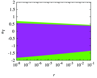
Figure 2: The shaded regions in the $r$–$n_{T}$ plane are those allowed from the constraint $\left|\rho_{\rm GW}^{(IR)}\right|/\rho_{c}<1$ considering super-Hubble fluctuations. The analysis is for the RD phase. The case assuming an evolution of $H$ during inflation according to Eq. (71) is shown in purple. On the other hand, the case where we assume that $H$ is constant during inflation is shown in green. $N_{\ast}=60$ is assumed in this figure.

V Effects of Sub-Hubble Modes

We now turn to the discussion of the effects of sub-Hubble modes. We focus on the radiation and matter epochs. Note that in an early de Sitter phase the sub-Hubble modes are in their vacuum state and hence yield no back-reaction effects.

The general expression for the energy density in the totality of sub-Hubble modes is

$$\rho_{\rm GW}^{\rm(UV)}\,=\,\frac{1}{8\pi Ga^{2}}\int_{k_{\rm hor}}^{k_{\rm max}}\frac{dk}{k}\frac{\rho_{\rm GW}(k)}{|A_{k}|^{2}}{\cal P}_{\rm prim}(k),$$ (82)

Inserting the expression (62) for the power spectrum and the short wavelength solutions of the mode functions $h_{k}$ into the general expression (27), we obtain, for RD epoch

$$\rho_{\rm{GW}}^{\rm{(UV)}}(t)\, = \,\frac{1}{8\pi G}\left(\frac{a_{\rm ref}}{a}\right)^{4}H_{\rm ref}^{2}\frac{A_{T}(k_{*})}{8}{\rm{log}}\left(\frac{k_{\rm{max}}}{k_{\rm{hor}}}\right)\,\,\,({\rm{for}}\,\,\,n_{T}=0)\,,$$ (83)

$$= \,\frac{1}{8\pi G}\left(\frac{a_{\rm ref}}{a}\right)^{4}H_{\rm ref}^{2}\frac{1}{n_{T}}\frac{A_{T}(k_{*})}{8}\left[\left(\frac{k_{\rm{max}}}{k_{*}}\right)^{n_{T}}-\left(\frac{k_{\rm{hor}}}{k_{*}}\right)^{n_{T}}\right]\,\,\,({\rm{for}}\,\,\,n_{T}\neq 0)\,,$$ (84)

where $a_{\rm ref}$ is the value of the scale factor at some reference time, and $H_{\rm ref}$ is the Hubble rate at that time. Expressing the result in terms of the critical energy density $\rho_{c}(t)$ this becomes

$$\rho_{\rm{GW}}^{\rm{(UV)}}(t)\, = \,\frac{1}{3}\rho_{c}(t)\frac{A_{T}(k_{*})}{8}{\rm{log}}\left(\frac{k_{\rm{max}}}{k_{\rm{hor}}}\right)\,\,\,({\rm{for}}\,\,\,n_{T}=0)\,,$$ (85)

$$= \,\frac{1}{3}\rho_{c}(t)\ \frac{A_{T}(k_{*})}{8n_{T}}\left[\left(\frac{k_{\rm{max}}}{k_{*}}\right)^{n_{T}}-\left(\frac{k_{\rm{hor}}}{k_{*}}\right)^{n_{T}}\right]\,\,\,({\rm{for}}\,\,\,n_{T}\neq 0)\,,$$ (86)

As expected, this energy density is positive and scales as radiation. For $n_{T}>0$ the shortest wavelength modes dominate the contribution, and the relative contribution of gravitational waves to the energy density is (modulo subdominant terms) constant in time. On the other hand, for $n_{T}<0$, the contribution of short wavelength gravitational waves to the total energy density grows in time since $k_{\rm{hor}}(t)$ is a decreasing function of time. In either case, $\rho_{\rm{GW}}^{\rm{(UV)}}$ takes the largest value for $k_{\rm max}=k_{R}$ and $k_{\rm hor}=k_{\rm eq}$.

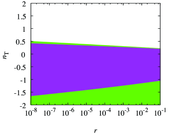
Figure 3: The shaded regions in the $r$–$n_{T}$ plane are those allowed from the constraint $\Omega_{\rm GW}\left(=\left|\rho_{\rm GW}^{(IR)}\right|/\rho_{c}\right)<1.5\times 10^{-5}$ for short wavelength modes in the RD phase. The case assuming an evolution of $H$ during inflation according to Eq. (71) is shown in purple. On the other hand, the case where we assume that $H$ is constant during inflation is shown in green. $N_{\ast}=60$ is assumed in this figure.

Short wavelength gravitational waves contribute to the effective number of degrees of freedom of radiation. Nucleosynthesis constrains this number quite tightly (see e.g. NSconstraints for a review). The nucleosynthesis constraint on the relative contribution $\Omega_{\rm{GW}}$ is

$$\Omega_{\rm{GW}}\,<\,1.5\times 10^{-5}\,.$$ (88)

In Fig. 3, we show the region of $\rho_{\rm{GW}}^{\rm{(UV)}}<1.5\times 10^{-5}\rho_{c}$ by taking $k_{\rm max}=k_{R}$ and $k_{\rm hor}=k_{\rm eq}$. In particular, the bound on the tilt of the tensor spectrum becomes

$$n_{T}\,<0.2\,$$ (89)

if the tensor to scalar ratio is taken to be $r=10^{-1}$. This is consistent with the result in the first reference of Stewart , where a value of $r\sim 1$ was used and the UV cutoff was taken to be at the Planck scale. Like in the case for super-Hubble modes, when the evolution of the Hubble parameter during inflation is taken into account by using Eq. (71), a red-tilted spectrum can also be constrained as $n_{T}\gtrsim-1.1$ for $r\sim 0.01$.

As discussed in Stewart , the current limits on the tilt $n_{T}$ from other searches for gravitational waves such as direct detection experiments (LIGO) or pulsar timing arrays yield weaker bounds on $n_{T}$ since these experiments are less sensitive to the high frequency waves which dominate for positive values of the tilt.

Next we look at the case in the MD phase. Assuming that $n_{T}<2$, we obtain

$$\rho_{\rm GW}^{\rm(UV)} = \frac{1}{8\pi G}\frac{a_{R}^{6}H_{R}^{4}}{a^{4}k_{\ast}^{2}}\frac{9}{8\cdot 16}\frac{1}{2-n_{T}}\frac{A_{T}(k_{\ast})}{4}\left[\left(\frac{k_{\rm max}}{k_{\ast}}\right)^{n_{T}-2}-\left(\frac{k_{\rm hor}}{k_{\ast}}\right)^{n_{T}-2}\right]$$ (90)

$$= \frac{\rho_{c}(t)}{3}\frac{9}{8\cdot 16}\frac{A_{T}(k_{\ast})}{2-n_{T}}\left[\left(\frac{k_{\rm hor}}{k_{\ast}}\right)^{n_{T}}-\left(\frac{k_{\rm hor}}{k_{\rm max}}\right)^{2}\left(\frac{k_{\rm max}}{k_{\ast}}\right)^{n_{T}}\right].$$

We can also constrain $n_{T}$ and $r$ by using the same argument as for the RD case. In fact, for the MD case, when $n_{T}>0$, $\rho_{\rm GW}^{\rm(UV)}$ gets largest for $k_{\rm hor}=k_{\rm eq}$. On the other hand, when $n_{T}<0$, the case of $k_{\rm hor}=k_{0}$ gives the maximum value of $\rho_{\rm GW}^{\rm(UV)}$. Therefore, to get a constraint on $n_{T}$ and $r$, we take $k_{\rm hor}=k_{\rm eq}$ and $k_{0}$ for $n_{T}>0$ and $<0$, respectively. Since the constraint on $n_{T}$ and $r$ from the MD case is similar to the one from the RD case, we do not show the plot here.

VI Conclusions and Discussion

In this paper we have re-visited the back-reaction effects of sub- and super-Hubble modes of gravitational waves on the background cosmology. In agreement with previous works Abramo2 we find that super-Hubble induce a negative energy density and have an equation of state which corresponds to curvature. We find that if the tensor spectrum is blue (i.e. $n_{T}>0$), then by demanding that the energy density in the early universe is not dominated by curvature leads to some constraints. In the case of an inflationary universe, it leads to a constraint on the total number of $e$-foldings which depends on the value of $n_{T}$ (see (67)), and in the case of the radiation phase it leads to a constraint on the tensor index $n_{T}$ which depends on the energy scale at the beginning of the radiation phase (see (70)). In both cases, the bounds depend on the tensor to scalar ratio at the pivot scale $k_{*}$.

The energy density in sub-Hubble gravitational waves (which behave like normal radiation) is constrained by the nucleosynthesis bound (88). If the tensor spectrum is blue, this leads to constraints of the gravitational wave spectrum parameters $r$ and $n_{T}$ which are given by Eq. (85) and depicted graphically in Figure 3. When the evolution of the Hubble parameter during inflation is taken into account (see Eq. (71)), which is the case for usual slow-roll inflationary models, we can also obtain a lower bound on $n_{T}$ from the the above argument (see Figs. 2 and 3).

References

- (1) A. A. Starobinsky, “Spectrum of relict gravitational radiation and the early state of the universe,” JETP Lett. 30 (1979) 682 [Pisma Zh. Eksp. Teor. Fiz. 30 (1979) 719].
-
(2)
A. Guth, “The Inflationary Universe: A Possible Solution
To The Horizon And Flatness Problems,” Phys. Rev. D 23, 347
(1981);
R. Brout, F. Englert and E. Gunzig, “The Creation Of The Universe As A Quantum Phenomenon,” Annals Phys. 115, 78 (1978);
A. A. Starobinsky, “A New Type Of Isotropic Cosmological Models Without Singularity,” Phys. Lett. B 91, 99 (1980);
K. Sato, “First Order Phase Transition Of A Vacuum And Expansion Of The Universe,” Mon. Not. Roy. Astron. Soc. 195, 467 (1981);
L. Z. Fang, “Entropy Generation in the Early Universe by Dissipative Processes Near the Higgs’ Phase Transitions,” Phys. Lett. B 95, 154 (1980). -
(3)
R. H. Brandenberger, A. Nayeri, S. P. Patil and C. Vafa,
“Tensor Modes from a Primordial Hagedorn Phase of String Cosmology,”
Phys. Rev. Lett. 98, 231302 (2007)
[hep-th/0604126];
R. H. Brandenberger, A. Nayeri and S. P. Patil, “Closed String Thermodynamics and a Blue Tensor Spectrum,” Phys. Rev. D 90, no. 6, 067301 (2014) [arXiv:1403.4927 [astro-ph.CO]]. - (4) R. H. Brandenberger and C. Vafa, “Superstrings In The Early Universe,” Nucl. Phys. B 316, 391 (1989).
-
(5)
R. H. Brandenberger, “String Gas Cosmology: Progress
and Problems,” Class. Quant. Grav. 28, 204005 (2011)
[arXiv:1105.3247 [hep-th]];
R. H. Brandenberger, “String Gas Cosmology,” String Cosmology, J.Erdmenger (Editor). Wiley, 2009. p.193-230 [arXiv:0808.0746 [hep-th]];
T. Battefeld and S. Watson, “String gas cosmology,” Rev. Mod. Phys. 78, 435 (2006) [arXiv:hep-th/0510022]. - (6) P. A. R. Ade et al. [BICEP2 and Keck Array Collaborations], “Improved Constraints on Cosmology and Foregrounds from BICEP2 and Keck Array Cosmic Microwave Background Data with Inclusion of 95 GHz Band,” Phys. Rev. Lett. 116, 031302 (2016) [arXiv:1510.09217 [astro-ph.CO]].
-
(7)
A. Stewart and R. Brandenberger,
“Observational Constraints on Theories with a Blue Spectrum of Tensor Modes,”
JCAP 0808, 012 (2008)
[arXiv:0711.4602 [astro-ph]];
R. Camerini, R. Durrer, A. Melchiorri, A. Riotto, R. Durrer, A. Melchiorri and A. Riotto, “Is cosmology compatible with blue gravity waves?,” Phys. Rev. D 77, 101301 (2008) [arXiv:0802.1442 [astro-ph]];
S. Kuroyanagi, T. Takahashi and S. Yokoyama, “Blue-tilted Tensor Spectrum and Thermal History of the Universe,” JCAP 1502, 003 (2015) [arXiv:1407.4785 [astro-ph.CO]];
G. Cabass, L. Pagano, L. Salvati, M. Gerbino, E. Giusarma and A. Melchiorri, “Updated Constraints and Forecasts on Primordial Tensor Modes,” Phys. Rev. D 93, no. 6, 063508 (2016) [arXiv:1511.05146 [astro-ph.CO]]. - (8) S. R. Green and R. M. Wald, “How well is our universe described by an FLRW model?,” Class. Quant. Grav. 31, 234003 (2014) [arXiv:1407.8084 [gr-qc]].
- (9) F. Finelli and R. H. Brandenberger, “Parametric amplification of gravitational fluctuations during reheating,” Phys. Rev. Lett. 82, 1362 (1999) [hep-ph/9809490].
- (10) V. F. Mukhanov, L. R. W. Abramo and R. H. Brandenberger, “On the Back reaction problem for gravitational perturbations,” Phys. Rev. Lett. 78, 1624 (1997) [gr-qc/9609026].
- (11) L. R. W. Abramo, R. H. Brandenberger and V. F. Mukhanov, “The Energy - momentum tensor for cosmological perturbations,” Phys. Rev. D 56, 3248 (1997) [gr-qc/9704037].
- (12) R. H. Brandenberger, “Back reaction of cosmological perturbations and the cosmological constant problem,” hep-th/0210165.
-
(13)
A. M. Polyakov,
“Infrared instability of the de Sitter space,”
arXiv:1209.4135 [hep-th];
A. M. Polyakov, “Decay of Vacuum Energy,” Nucl. Phys. B 834, 316 (2010) [arXiv:0912.5503 [hep-th]];
A. M. Polyakov, “De Sitter space and eternity,” Nucl. Phys. B 797, 199 (2008) [arXiv:0709.2899 [hep-th]]. -
(14)
N. C. Tsamis and R. P. Woodard,
“Relaxing the cosmological constant,”
Phys. Lett. B 301, 351 (1993);
N. C. Tsamis and R. P. Woodard, “Quantum gravity slows inflation,” Nucl. Phys. B 474, 235 (1996) [hep-ph/9602315];
N. C. Tsamis and R. P. Woodard, “Comment on ‘Can infrared gravitons screen Lambda?’,” Phys. Rev. D 78, 028501 (2008) [arXiv:0708.2004 [hep-th]]. -
(15)
N. C. Tsamis and R. P. Woodard,
“The Physical basis for infrared divergences in inflationary quantum gravity,”
Class. Quant. Grav. 11, 2969 (1994);
N. C. Tsamis and R. P. Woodard, “The Quantum gravitational back reaction on inflation,” Annals Phys. 253, 1 (1997) [hep-ph/9602316]. - (16) W. Unruh, “Cosmological long wavelength perturbations,” astro-ph/9802323.
- (17) G. Geshnizjani and R. Brandenberger, “Back reaction and local cosmological expansion rate,” Phys. Rev. D 66, 123507 (2002) [gr-qc/0204074].
- (18) L. R. Abramo and R. P. Woodard, “No one loop back reaction in chaotic inflation,” Phys. Rev. D 65, 063515 (2002) [astro-ph/0109272].
- (19) G. Geshnizjani and R. Brandenberger, “Back reaction of perturbations in two scalar field inflationary models,” JCAP 0504, 006 (2005) [hep-th/0310265].
- (20) G. Marozzi, G. P. Vacca and R. H. Brandenberger, “Cosmological Backreaction for a Test Field Observer in a Chaotic Inflationary Model,” JCAP 1302, 027 (2013) [arXiv:1212.6029 [hep-th]].
- (21) R. H. Brandenberger and C. S. Lam, “Back-reaction of cosmological perturbations in the infinite wavelength approximation,” hep-th/0407048.
- (22) V. F. Mukhanov, H. A. Feldman and R. H. Brandenberger, “Theory of cosmological perturbations. Part 1. Classical perturbations. Part 2. Quantum theory of perturbations. Part 3. Extensions,” Phys. Rept. 215, 203 (1992).
- (23) R. H. Brandenberger, “Lectures on the theory of cosmological perturbations,” Lect. Notes Phys. 646, 127 (2004) [arXiv:hep-th/0306071].
- (24) P. Martineau and R. H. Brandenberger, “The Effects of gravitational back-reaction on cosmological perturbations,” Phys. Rev. D 72, 023507 (2005) [astro-ph/0505236].
- (25) N. Bartolo, E. Komatsu, S. Matarrese and A. Riotto, “Non-Gaussianity from inflation: Theory and observations,” Phys. Rept. 402, 103 (2004) [astro-ph/0406398].
- (26) C. Kiefer, D. Polarski and A. A. Starobinsky, “Quantum to classical transition for fluctuations in the early universe,” Int. J. Mod. Phys. D 7, 455 (1998) [gr-qc/9802003].
- (27) P. Martineau, “On the decoherence of primordial fluctuations during inflation,” Class. Quant. Grav. 24, 5817 (2007) [astro-ph/0601134].
- (28) T. Kobayashi, M. Yamaguchi and J. Yokoyama, “G-inflation: Inflation driven by the Galileon field,” Phys. Rev. Lett. 105, 231302 (2010) [arXiv:1008.0603 [hep-th]].
- (29) J. Khoury, B. A. Ovrut, P. J. Steinhardt and N. Turok, “The Ekpyrotic universe: Colliding branes and the origin of the hot big bang,” Phys. Rev. D 64, 123522 (2001) [hep-th/0103239].
- (30) M. Gasperini and G. Veneziano, “Pre - big bang in string cosmology,” Astropart. Phys. 1, 317 (1993) [hep-th/9211021].
- (31) M. Maggiore, “Gravitational wave experiments and early universe cosmology,” Phys. Rept. 331, 283 (2000) [gr-qc/9909001].
- (32) R. H. Cyburt, B. D. Fields, K. A. Olive and T. H. Yeh, “Big Bang Nucleosynthesis: 2015,” Rev. Mod. Phys. 88, 015004 (2016) [arXiv:1505.01076 [astro-ph.CO]].