Multiscale properties of Large Eddy Simulations:
correlations between resolved-scale velocity-field increments and subgrid-scale quantities

Abstract

We provide analytical and numerical results concerning multi-scale correlations between the resolved velocity field and the subgrid-scale (SGS) stress-tensor in large eddy simulations (LES). Following previous studies for Navier-Stokes equations (NSE), we derive the exact hierarchy of LES equations governing the spatio-temporal evolution of velocity structure functions of any order. The aim is to assess the influence of the sub-grid model on the inertial range intermittency. We provide a series of predictions, within the multifractal theory, for the scaling of correlation involving the SGS stress and we compare them against numerical results from high-resolution Smagorinsky LES and from a-priori filtered data generated from direct numerical simulations (DNS). We find that LES data generally agree very well with filtered DNS results and with the multifractal prediction for all leading terms in the balance equations. Discrepancies are measured for some of the subleading terms involving cross-correlation between resolved velocity increments and the SGS tensor or the SGS energy transfer, suggesting that there must be room to improve the SGS modelisation to further extend the inertial range properties for any fixed LES resolution.

1 Introduction

One of the main challenges in numerical and experimental turbulence is the existence of anomalously strong non-Gaussian fluctuations, which are a generic feature of all three-dimensional flows [1, 2, 3]. Such extreme events occur in a variety of flow configurations, both on Eulerian and Lagrangian domains [4, 5, 6, 7, 8, 9] and become more and more important with increasing Reynolds number, $Re=U_{0}L_{0}/\nu$, where $U_{0},L_{0}$ are the characteristic velocity and length scale of the flow, while $\nu$ is the viscosity. The Reynolds number measures the relative importance of linear vs non-linear terms in the Navier-Stokes evolution. For large $Re$, the dynamics becomes fully turbulent and an inertial-range energy cascade develops. Power laws with anomalous scaling exponents are observed for moments of velocity increments in the inertial range, a phenomenon known as intermittency. No systematic derivation of the value of the scaling exponents is known from first principle, and the problem is considered key for both fundamental aspects and its applied consequences, being connected to the existence of wild fluctuations in the velocity increments and in the energy dissipation field. Empirical data are always affected by spurious and/or sub-leading contributions, making an accurate determination of the scaling exponents difficult. Hence, it is mandatory to develop more and more refined experimental and numerical techniques to increase the scaling range and/or to improve the scaling properties. State-of-the-art data in the laboratories reach a maximum inertial range extensions of one/two decades [10], and the exponents are often evaluated using sophisticated finite-size-techniques as Extended Self Similarity [11] in order to reduce spurious effects. Similarly, concerning numerical studies, despite the huge progresses made in recent years [12, 13, 14] we are still far from reaching a resolution high enough to give a firm statement about scaling, in particular concerning subtle issues connected to the alleged different statistical properties of longitudinal and transverse velocity increments, or of the enstrophy and stress.

A potential alternative strategy to minimise viscous effects and to concentrate only on high Reynolds number properties is provided by the application of large eddy simulation (LES), where we introduce a model for the small-scale dynamics while fully resolving the most energy-containing scales [15, 16, 17, 18, 2, 19, 20, 3, 21, 22, 23, 24, 25]. In this paper, we perform a first step in order to assess how much LES can be used to estimate inertial range scaling properties of fully developed turbulence. The aim being twofold, first to have a tool able to minimise viscous and small-scale effects on the inertial range, second to assess the performance of high Reynolds LES tout-court owing to the emergent role of high-resolution modelling where the cutoff scale lies in the inertial subrange [26, 27].

In order to assess the performance of LES models in reproducing the aforementioned extreme events with reasonable accuracy, it is first mandatory to understand the statistical coupling between the resolved velocity field and the subgrid model. The present paper is mainly concerned with this point. To do that, we derive the exact hierarchy of equations satisfied by the generic $n$th order structure functions made in terms of moments of the resolved velocity increments and involving the correlations with the modelled subgrid-scale (SGS) stress-tensor. Furthermore, we provide a set of multifractal (MF) predictions for the scaling behavior of all correlations entering in the equations of motion, which are subsequently compared to data obtained from a-priori filtered direct numerical simulations (DNS) of homogeneous isotropic turbulence on up to $2048^{3}$ grid points and from a-posteriori highly resolved Smagorinsky LES using up to $1024^{3}$ grid points. We focus here on the Smagorinsky model party because of its simplicity and wide usage. More importantly, the Smagorinsky model is unable to model interactions leading to backscatter events. As most LES models include a dissipative part to prevent numerical instabilities, the modelling of backscatter events is still a challenge in LES. In view of potential applicability of LES models to study inertial-range physics, we also wish to assess if and how the absence of backscatter affects the scaling of the correlation functions, and the Smagorinsky model is particularly well suited to this part of the analysis.
The main conclusion is that already the Smagorinsky LES modelling is a good tool to minimise effects induced by the ultraviolet, large wavenumber, cut-off on the inertial range: all leading scaling properties measured on the real a-priori data are well reproduced by the a-posteriori LES data. This opens the way to perform highly resolved LES to improve the actual knowledge of the inertial range physics, by further minimising the dissipative effects. For the sake of simplicity, we start here to address only homogeneous and isotropic turbulence but the whole machinery can be reproduced for bounded flows as well, at the price of a higher analytical complexity.
This paper is organised as follows. The structure function hierarchies are derived in Sec. 2 and in Appendix A and B for different formulations of the filtered Navier-Stokes equations (NSE). Section 3 is concerned with the predictions for scaling behaviour of multi-points correlation functions based on the MF hypothesis. The numerical results are presented in Sec. 4, and we conclude with a summary in Sec. 5.

2 Structure function hierarchies for LES

The application of LES requires a splitting into resolved scales and unresolved (subgrid) scales. The resolved-scale quantities are defined though the application of a filter kernel $G^{\Delta}$ at a given scale scale $\Delta$ to the velocity field ${\bf v}$

$$\overline{{\bf v}}({\bf x},t)\equiv\int_{\Omega}d{\bf y}\ G^{\Delta}(|{\bf x}-{\bf y}|){\bf v}({\bf y},t)\ ,$$ (1)

where $\Omega$ is the domain of definition of ${\bf v}$, while for the sake of concreteness one can think $G^{\Delta}$ as given by a projection operation in Fourier space, i.e. through spherically symmetric Galerkin truncation for all wavenumbers such that $k>2\pi/\Delta$.

In order to derive a hierarchy of equations relating the structure and correlation functions applicable to LES, we consider the filtered incompressible NSE on a three-dimensional domain $\Omega=[0,L]^{3}$ with periodic boundary conditions

$$\partial_{t}\overline{v}_{i}+\partial_{j}(\overline{v}_{i}\overline{v}_{j}+\overline{P}\delta_{ij}+\tau^{\Delta}_{ij})=f_{i}\ ,$$ (2)

$$\partial_{i}\overline{v}_{i}=0\ ,$$ (3)

where $P$ denotes the pressure, $\bm{f}$ the external force and $\tau^{\Delta}_{ij}=\overline{v_{i}v_{j}}-\overline{v}_{i}\overline{v}_{j}$ the SGS stress tensor, which is replaced by a model in LES applications. The density has been set to unity for convenience, and the contribution of the viscous term is neglected. The filter scale $\Delta$ is assumed to be smaller than the forcing scale $L_{f}$, such that $\overline{\bm{f}}=\bm{f}$.
The aim of this paper is to study the exact equations that must be satisfied by the velocity structure functions, i.e. the moments of the resolved velocity-field increments

$$\delta_{\bf r}\overline{{\bf v}}({\bf x})=\overline{{\bf v}}({\bf x}+{\bf r})-\overline{{\bf v}}({\bf x})\ .$$ (4)

The equation for the second-order correlation function, $\langle\delta_{{\bf r}}\overline{v}_{i}\delta_{\bf r}\overline{v}_{j}\rangle$, has been already derived in [28]. Here, we will further extend the previous results by generalising the exact hierarchy to moments of any order and by studying the relative importance of the different contributions entering in the corresponding equations of motion by using a-priori and a-posteriori LES at high resolution. The general evolution equation for the $n^{th}$-order correlation tensor consisting of velocity field differences is derived from the momentum balance at points ${\bf x}$ and ${\bf x}^{\prime}={\bf x}+{\bf r}$. Assuming homogeneity, we can make a change of variables ${\bf X}=\frac{1}{2}({\bf x}+{\bf x}^{\prime})\ \mbox{ and }\ {\bf r}={\bf x}^{\prime}-{\bf x}\ ,$ and dropping all dependencies from ${\bf X}$ in the averaged quantities. Furthermore, the partial derivatives with respect to ${\bf x}^{\prime}$- and ${\bf x}$-coordinates will be written as $\partial_{i}^{\prime}\equiv\partial_{x^{\prime}_{i}}\ ,\partial_{i}\equiv\partial_{x_{i}}\ ,$ and homogeneity implies $\partial_{i}^{\prime}=\partial_{r_{i}}=\partial_{i}$. Using the aforementioned results, one obtains the following evolution equation for the $n^{th}$-order correlation tensor for homogeneous isotropic turbulence

$$\partial_{t}\langle\delta_{r}\overline{v}_{i_{1}}\ldots\delta_{r}\overline{v}_{i_{n}}\rangle= -\partial_{k}\langle\delta_{r}\overline{v}_{i_{1}}\ldots\delta_{r}\overline{v}_{i_{n}}\delta_{r}\overline{v}_{k}\rangle$$

$$-\frac{1}{|S_{n-1}|}\sum_{\sigma\in S_{n}}\langle\delta_{r}\overline{v}_{i_{\sigma(1)}}\ldots\delta_{r}\overline{v}_{i_{\sigma(n-1)}}\delta_{r}(\partial_{k}\overline{P}\delta_{ki_{\sigma(n)}})\rangle$$

$$+\frac{1}{|S_{n-1}|}\sum_{\sigma\in S_{n}}\langle\delta_{r}\overline{v}_{i_{\sigma(1)}}\ldots\delta_{r}\overline{v}_{i_{\sigma(n-1)}}\delta_{r}f_{i_{\sigma(n)}}\rangle$$

$$-\frac{1}{|S_{n-1}|}\sum_{\sigma\in S_{n}}\langle\delta_{r}\overline{v}_{i_{\sigma(1)}}\ldots\delta_{r}\overline{v}_{i_{\sigma(n-1)}}\delta_{r}(\partial_{k}\tau^{\Delta}_{ki_{\sigma(n)}})\rangle\ ,$$ (5)

where $S_{n}$ denotes the symmetric group in $n$ elements, that is, we sum over all permutations of the indices $i_{1},\ldots,i_{n}$. In order to avoid counting identical terms involving products of $n-1$ velocity field increments multiple times, it is necessary to divide the sum over all permutations in $S_{n}$ by the number of elements of $S_{n-1}$ denoted by $|S_{n-1}|$.
It is important to stress that a similar hierarchy of equations for the structure functions corresponding to the full Navier-Stokes evolution was derived in two different ways in [29] and in [30]. For comparison, the first two lines of eq. (2) are identical to eq. (3.1) in Ref. [30] obtained for the Navier-Stokes evolution, except for the absence of viscous terms in our case. The additional terms present in eq. (2) describe the effect of the forcing in the third line and the correlations between the velocity-field increments and the SGS tensor in the last line. This last term is the core object in the present paper, and our aim is study its scaling properties and its role in the balance equations. In the evolution equation for correlation tensors derived from the original NSE, the correlation with the viscous stress appears with the same structure as the correlation with the SGS-stress in Eq. (2). The hierarchy of equations in [30] was derived from kinematic constraints only. These are: the geometric constraints, i.e. restrictions on the form of the correlation tensors due to their invariance under rotations and reflections, and incompressibility. Since no dynamical information was used in the derivation of the hierarchy for the full Navier-Stokes evolution, the algebraic structure of the LES hierarchy is exactly the same. Furthermore, the additional correlation tensor in eq. (2) must also obey the same kinematic constraints as the velocity increment tensors. Hence, in order to derive the LES hierarchy relating structure functions of any order, the only necessary work lies in the evaluation of the correlation tensors involving the SGS-stress,

$$H_{i_{1}\ldots i_{n}}\equiv\frac{1}{|S_{n-1}|}\sum_{\sigma\in S_{n}}\langle\delta_{r}\overline{v}_{i_{\sigma(1)}}\ldots\delta_{r}\overline{v}_{i_{\sigma(n-1)}}\delta_{r}(\partial_{k}\tau^{\Delta}_{ki_{\sigma(n)}})\rangle\ .$$ (6)

The necessary calculations are summarised in Appendix A. Let us first introduce some general notations for the correlation functions that will be met during the calculations. By restricting our analysis to homogeneous and isotropic turbulence we can characterise all velocity correlation functions in terms of longitudinal and $\delta_{r}v_{L}=(\overline{{\bf v}}({\bf x}+{\bf r})-\overline{{\bf v}}({\bf x}))\cdot{\bf r}/r$ and the transverse, $\delta_{r}v_{N}$, components, where the latter is any component of the vector $\delta_{r}\overline{{\bf v}}_{N}=\delta_{r}\overline{{\bf v}}-\delta_{r}v_{L}{\bf r}/r$. We will denote the correlation function made of $m$ longitudinal and $n$ transverse velocity increments at scale $r$ as:

$$D^{n,m}(r)\equiv\langle(\delta_{r}\overline{v}_{L})^{n}(\delta_{r}\overline{v}_{N})^{m}\rangle\ ,$$ (7)

and the multi-scale correlation functions including also the components of the SGS stress tensor as:

$$G^{n,m}_{i,j}(r,\Delta)\equiv\langle(\delta_{r}\overline{v}_{L})^{n}(\delta_{r}\overline{v}_{N})^{m}\tau^{\Delta}_{ij}\rangle\ .$$ (8)

It will be useful to introduce also two more quantities for correlation functions similar to Eq. (8), namely:

$$S^{n}_{i,j}(r,\Delta)=\langle(\delta_{r}\overline{v}_{L})^{n}\tau^{\Delta}_{ki}\partial_{k}\overline{v}_{j}\rangle\ ,$$ (9)

and

$$T^{n}_{i,j}(r,\Delta)=\langle(\delta_{r}\overline{v}_{L})^{n}\tau^{\Delta}_{ki}\partial_{k}^{\prime}\overline{v}_{j}^{\prime}\rangle\ ,$$ (10)

where for the last two cases for the sake of simplicity we have introduced only the longitudinal velocity increments (for the set of exact equations we are going to analyse in this paper it turns out that this choice is not restrictive). Finally, the pressure correlations are denoted as

$$P^{n}(r,\Delta)=\langle(\delta_{r}\overline{v}_{L})^{n}\delta_{r}(\partial_{i}\overline{P}\delta_{iL})\ \rangle\ .$$ (11)

Let us note that we have retained the dependencies on $r$ and $\Delta$ as appropriate, in order to stress the explicit dependencies on the sub-grid stress tensor and on its characteristic scale $\Delta$ when relevant. After some algebra, one derives the exact hierarchy obtained for the evolution of the general longitudinal $n^{\rm th}$ order structure function, $\partial_{t}D^{n,0}(r)$ (see Appendix A and also [30, 29] for similar derivation obtained for the case of NSE):

$$\partial_{t}D^{n,0}(r)= -\left(\partial_{r}D^{n+1,0}(r)+\frac{2}{r}D^{n+1,0}(r)-\frac{2n}{r}D^{n-1,2}(r)\right)$$

$$-2n\left(\partial_{r}+\frac{2}{r}\right)G^{n-1,0}_{L,L}(r,\Delta)+\frac{4n}{r}(G^{n-2,1}_{L,N}(r,\Delta)+G^{n-1,0}_{N,N}(r,\Delta))$$

$$+\frac{2n!}{(n-2)!}(S^{n-2}_{L,L}(r,\Delta)+T^{n-2}_{L,L}(r,\Delta))-2nP^{n}(r,\Delta)+2nF^{n}(r)\ ,$$ (12)

where the correlations involving the forcing $F^{n}(r)$ are described in Appendix A. The form and properties of the correlation tensors are discussed in detail in Appendix C.1 for those leading to the functions $G^{n-1,0}_{L,L}(r,\Delta)$, $G^{n-1,0}_{N,N}(r,\Delta)$ and, $G^{n-2,1}_{L,N}(r,\Delta)$. The functions $T^{n-2}_{L,L}(r,\Delta)$ and $S^{n-2}_{L,L}(r,\Delta)$ including their common combinatorial prefactor are treated in Appendix C.2, and the pressure correlations are contained in Appendix C.3. A similar set of equations can also be obtained for the evolution of the most general mixed longitudinal-transverse case, $D^{n,m}(r)$.
Let us notice that not all terms are always present, as one can explicitly see by rewriting the above relation for the first low order moments, $n=2$ (corresponding to the Monin-Kármán-Howarth energy balance equation), $n=3$ and $n=4$:

$$\partial_{t}D^{2,0}(r)= -\left(\partial_{r}+\frac{4}{r}\right)\left(\frac{1}{3}D^{3,0}(r)+G^{1,0}_{L,L}(r,\Delta)\right)+4S^{0}_{L,L}(\Delta)+4F^{2}\ ,$$ (13)

$$\partial_{t}D^{3,0}(r)= -\left(\partial_{r}+\frac{2}{r}\right)D^{4,0}(r)+\frac{6}{r}D^{2,2}(r)-6\left(\partial_{r}+\frac{2}{r}\right)G^{2,0}_{L,L}(r,\Delta)$$

$$+\frac{12}{r}(G^{1,1}_{L,N}(r,\Delta)+G^{2,0}_{N,N}(r,\Delta))+12(S^{1}_{L,L}(r,\Delta)+T^{1}_{L,L}(r,\Delta))$$

$$-6P^{3}(r,\Delta)+6F^{3}(r)\ ,$$ (14)

$$\partial_{t}D^{4,0}(r)= -\left(\partial_{r}+\frac{2}{r}\right)D^{5,0}(r)+\frac{8}{r}D^{3,2}(r)-8\left(\partial_{r}+\frac{2}{r}\right)G^{3,0}_{L,L}(r,\Delta)$$

$$+\frac{16}{r}(G^{2,1}_{L,N}(r,\Delta)+G^{3,0}_{N,N}(r,\Delta))+24(S^{2}_{L,L}(r,\Delta)+T^{2}_{L,L}(r,\Delta))$$

$$-8P^{4}(r,\Delta)+8F^{4}(r)\ .$$ (15)

Equation (13) stands out from the hierarchy as the terms $P^{2}(r,\Delta)$, $T^{2}_{L,L}(r,\Delta)$, $G^{1,0}_{N,N}(r,\Delta)$, $G^{0,1}_{L,N}(r,\Delta)$ and $D^{1,2}(r)$ are not present and the incompressibility constraint implies $P^{2}(r,\Delta)=0$ and $2D^{1,2}(r)/r=(\partial_{r}+2/r)D^{3,0}(r)$. $T^{2}(r,\Delta)$, $G^{1,0}_{N,N}(r,\Delta)$ and $G^{0,1}_{L,N}(r,\Delta)$ can be absorbed into the derivative of $G^{1,0}_{L,L}(r,\Delta)$; see Appendices A.1 and C.2 for further details. It is important to notice that the function $S^{n-2}_{L,L}(r,\Delta)$ for $n=2$ in Eq. (13) is not a function of $r$, i.e. it is not a real multi-scale function, since

$$S^{0}_{L,L}(\Delta)=\langle\tau^{\Delta}_{kL}\partial_{k}\tau_{kL}\rangle\$$ (16)

is proportional to the SGS energy transfer:

$$3S^{0}_{L,L}(\Delta)=\Pi(\Delta)=-\langle\tau^{\Delta}_{ki}\partial_{k}\overline{v}_{i}\rangle,$$

see Appendices A.1 and C.2 or Ref. [28], where Eq. (13) has been derived directly.

Before proceeding, let us make a few general comments about the structure of the different terms entering in Eq. (2). It is important to notice that the terms containing correlations of type $G^{\alpha,\beta}_{i,j}(r,\Delta)/r$ with $(\alpha,\beta)=(n-1,0),\,(n-2,1)$ and the term $S^{n-2}_{i,j}(r,\Delta)$ have the same physical dimensions but two completely different roles: the former consists of $n-1$ velocity-field increments multiplied by the SGS stress tensor, the latter consists of $n-1$ velocity-field increments multiplied by terms of the form $\tau^{\Delta}_{ki}\partial_{k}\overline{v}_{j}$ that contribute to the definition of the SGS energy transfer, $\Pi(\Delta)$. As a result, the latter will play a key role in the balancing of the hierarchy as suggested from the fact that also in the original NSE the presence of the dissipative anomaly is a signature of non-trivial multi-scale correlation functions among viscous and inertial scales. On the contrary, the terms labelled $T^{n-2}_{i,j}(r,\Delta)$ are not correlated to the local energy transfer being defined in terms of the SGS stress tensor and the velocity gradient at two different points ${\bf x}$ and ${\bf x}^{\prime}$.

3 Scaling of correlation functions

In this section, we will first assess the scaling properties of all terms entering in the previous hierarchy (2) from a phenomenological point of view. In Section 4, we will check using DNS and LES what is observed in reality and whether SGS modelling based on the Smagorinsky eddy viscosity is indeed able to reproduce the correct observations.
A popular and fruitful way to phenomenologically introduce intermittency in turbulence theory is to suppose that the velocity field is described by a MF process, where the velocity increment scales with a local Hölder exponent $h$, that is, $\delta_{r}v\sim r^{h}$, on a fractal set of dimension $D(h)$. Such phenomenological hypothesis has been used in the past to explain the observed anomalous scaling properties of the single-scale longitudinal and transverse velocity structure functions, the distribution of velocity gradients, of particles’ accelerations, velocity increments along particle trajectories and many other single and multi-scale turbulent properties [31, 32, 33, 12, 34, 35]. The simplest way to build up a MF-signal is to embed the velocity field into a multiplicative process, supposing that the velocity-field fluctuations at two nested, inertial-range, scales $r_{1}<r_{0}$ are connected by a scaling relation:

$$\delta_{r_{1}}v=\left(\frac{r_{1}}{r_{0}}\right)^{h}\delta_{r_{0}}v$$ (17)

and imagining that the successive breaking into eddies at smaller scale $r_{2}<r_{1}$ will be given by another multiplicative process with a different, but identically distributed, realisation of the local exponent, $h^{\prime}$ [36, 37, 38, 39]

$$\delta_{r_{2}}v=\left(\frac{r_{2}}{r_{1}}\right)^{h^{\prime}}\delta_{r_{1}}v.$$ (18)

Using this approach it is possible to predict the scaling behaviour for all terms entering in the hierarchy (2). We examine now the most important ones.

3.1 Single-scale Structure Functions $D^{n,m}(r)$

From the multiplicative MF Ansatz and by assuming that longitudinal and transverse increments do follow the same scaling distribution, it is straightforward to predict that [40]

$$D^{n,m}(r)\sim\int dh\left(\frac{r}{L_{0}}\right)^{h(m+n)}\left(\frac{r}{L_{0}}\right)^{3-D(h)}(\delta_{L_{0}}v)^{n+m}\sim A_{n,m}\left(\frac{r}{L_{0}}\right)^{\zeta_{n+m}}$$ (19)

where the last equality is obtained by estimating the integral in the saddle node approximation, $r\ll L_{0}\to\zeta(n+m)=\min_{h}(h(m+n)+3-D(h))$. The prefactors $A_{n,m}=O(1)$ are non-universal quantities which depend on the large-scale velocity distribution $\delta_{L_{0}}v$. One can immediately see that as soon as multiple realisations of the local Hölder exponent exist, the scaling properties are characterised by anomalous power laws, i.e. $\zeta(n)\neq n/3$. Nevertheless, it is important to notice that the MF approach contains the Kolmogorov K41 phenomenology as a limiting case, where the energy cascade is assumed to develop in a homogeneous way with a Hölder-$1/3$ velocity field everywhere in the three-dimensional volume, since $h=1/3$ and $D(1/3)=3$ imply $\zeta(n)=n/3$.

3.2 Multi-scale correlation functions and Fusion-Rules

Using the same approach, one can show that multi-scale correlation functions must also be characterised by anomalous scaling properties. For the generic two-scale correlation functions with $r<R$ we have the Fusion-Rules (FR) behaviour [41, 42, 43]:

$$\langle(\delta_{r}v)^{n}(\delta_{R}v)^{m}\rangle\sim\langle\left(\frac{r}{R}\right)^{n}(\delta_{R}v)^{n}(\delta_{R}v)^{m}\rangle\sim$$

$$\sim\int dhdh^{\prime}\left(\frac{r}{R}\right)^{hn+3-D(h)}\left(\frac{R}{L_{0}}\right)^{h^{\prime}(n+m)+3-D(h^{\prime})}$$

$$\sim\left(\frac{r}{R}\right)^{\zeta_{n}}\left(\frac{R}{L_{0}}\right)^{\zeta_{n+m}};\qquad r\ll R\ll L_{0}$$ (20)

where we have assumed a large separation among all scales, that $r$ and $R$ belong to the inertial range and we have applied a double saddle-node approximation of the integrals. Notice that Eq. (3.2) would correspond to the uncorrelated result iif the exponent follows K41, $\zeta_{n}=n/3$,

$$\langle(\delta_{r}v)^{n}(\delta_{R}v)^{m}\rangle\sim r^{n/3}R^{m/3}.$$ (21)

3.3 Multi-scale Correlation among velocity increments and SGS-stress, $G^{n,m}_{i,j}(r,\Delta)$

In order to introduce multi-scale correlation with the SGS stress tensor and the SGS energy dissipation entering in the hierarchy (2) we start from the observation made by [44, 45, 46] that the local SGS stress tensor can be estimated in terms of a suitable average of local velocity increments. As a result, for any Hölder-continuous velocity fields with local Hölder exponent $h$ one might estimate $\tau^{\Delta}$ to be a (local) MF-scaling function of the coarse-graining grid $\Delta$ [47, 48, 49, 50]:

$$\tau^{\Delta}_{ij}\sim\Delta^{2h}$$ (22)

Any correlation tensor involving velocity field increments at scale $r$ and the SGS-stress $\tau^{\Delta}_{ij}$ can therefore be treated as a correlation tensor involving the two scales $r$ and $\Delta$ within the Fusion-Rules approach. Following the same MF Ansatz of the previous section, we end up with:

$$\delta_{\Delta}\overline{v}_{L}\sim\left(\frac{\Delta}{r}\right)^{h}\delta_{r}\overline{v}_{L}\ .$$ (23)

For $\Delta<r$, the scaling behaviour of the correlations between the $n^{\rm th}$ power of a longitudinal velocity field increment and the SGS-stress can be estimated using Eq. (3.2):

$$\langle\tau^{\Delta}_{LL}(\delta_{r}\overline{v}_{L})^{n}\rangle\sim\left\langle(\delta_{\Delta}v_{L})^{2}(\delta_{r}\overline{v}_{L})^{n}\right\rangle\sim\left\langle\frac{\Delta^{2h}}{r^{2h}}(\delta_{r}\overline{v}_{L})^{n+2}\right\rangle\sim\left(\frac{\Delta}{r}\right)^{\zeta_{2}}\left(\frac{r}{L}\right)^{\zeta_{n+2}}\ ,$$ (24)

hence

$$\langle(\delta_{r}\overline{v}_{L})^{n}\tau^{\Delta}_{LL}\rangle\sim\left(\frac{\Delta}{L}\right)^{\zeta_{2}}\left(\frac{r}{L}\right)^{\zeta_{n+2}-\zeta_{2}}\ .$$ (25)

A few comments are now in order. First, the FR approach, being based on a MF multiplicative cascade, does not easily incorporate differences among scaling properties of longitudinal or transverse velocity increments. In fact, the most recent literature [14] shows that such a differences might disappear with increasing Reynolds numbers. Hereafter we will always assume that it is not important to distinguish among scaling properties of longitudinal, transverse or mixed longitudinal-transverse components, i.e. in all cases only the total number of velocity increment matters. Second, the FR estimate (24) is meant to capture only the leading power law behaviour and cannot take into account cancellations and symmetry constraints which may affect the prefactors. For example, the prediction (3.2) cannot hold for the special case of mixed longitudinal-transverse correlation with an odd power for the transverse increment, because in such a case $D^{n,2m+1}(r)=0,\,\forall m$ because of isotropy [51]. We will come back to this point in Sec. 4 where we analyse the data from DNS and LES. For the sake of comparison, it will be important to estimate the multi-scale correlation functions by assuming that the fields at different scales are almost decorrelated:

$$\langle(\delta_{r}\overline{v}_{L})^{n}\tau^{\Delta}_{LL}\rangle\sim\left\langle\Big{(}\frac{r}{L}\Big{)}^{nh}\Big{(}\frac{\Delta}{L}\Big{)}^{2h^{\prime}}\right\rangle\sim\left(\frac{r}{L}\right)^{\zeta_{n}}\left(\frac{\Delta}{L}\right)^{\zeta_{2}}\ .$$ (26)

Since $\zeta_{n+2}-\zeta_{2}<\zeta_{n}$ and $r/L<1$, the uncorrelated scaling Ansatz would be subleading with respect to that obtained from the MF cascade process. We will return to this point in Sec. 4.

3.4 Correlations between velocity field increments and components of the SGS-energy, $S^{n}_{i,j}(r,\Delta)$

The multiplicative cascade Ansatz can also be used to estimate the scaling behaviour of the correlations functions involving the components of the SGS-energy transfer

$$S^{n}_{i,j}=\langle\tau^{\Delta}_{ki}\partial_{k}\overline{v}_{j}(\delta_{r}\overline{v}_{L})^{n}\rangle.$$ (27)

As already noticed in the previous subsection, we will assume that no major scaling differences exist concerning the longitudinal or the transverse components of the different observables, and we proceed by applying the MF approach by specifying it for the case where all components are chosen in the longitudinal directions.

$$\langle\tau^{\Delta}_{LL}\partial_{x_{L}}\overline{v}_{L}(\delta_{r}\overline{v}_{L})^{n}\rangle \sim\left\langle(\delta_{\Delta}v_{L})^{2}\frac{\delta_{\Delta}v_{L}}{\Delta}(\delta_{r}\overline{v}_{L})^{n}\right\rangle\sim$$ (28)

$$\sim\left\langle\frac{\Delta^{3h-1}}{r^{3h}}(\delta_{r}\overline{v}_{L})^{n+3}\right\rangle\sim\frac{1}{\Delta}\left(\frac{\Delta}{r}\right)^{\zeta_{3}}\left(\frac{r}{L}\right)^{\zeta_{n+3}}\ .$$

Using the exact scaling property $\zeta_{3}=1$ one obtains

$$\langle\tau^{\Delta}_{kL}\partial_{k}\overline{v}_{L}(\delta_{r}\overline{v}_{L})^{n}\rangle\sim r^{-1}\langle(\delta_{r}\overline{v}_{L})^{n+3}\rangle\sim r^{\zeta_{n+3}-1}$$ (29)

hence, in the inertial-range scaling regime, all curves obtained at different $\Delta$ must collapse. Before summarising all results, let us mention that the scaling of the pressure terms, $P^{n}(r,\Delta)$ in Equation (2) will necessarily be connected to a mixing of all previous correlation functions, because it feels contributions from both the advection term $\overline{v}_{i}\partial_{i}\overline{v}_{j}$ and SGS tensor in Equation (2). On the contrary, one expects that the terms involving $T^{n}_{i,j}(r,\Delta)$ will always be sub-leading with respect to $S^{n}_{ij}(r,\Delta)$, because it consists of velocity gradients and SGS stress components in two different spatial locations.

More importantly, the above scaling relations tell us that the contribution involving the correlation with the components of the SGS energy transfer in Equation (2) are independent of $\Delta$ and they have the same contributions as the non-linear single-scale structure-function terms

$$\partial_{r}D^{n+1,0}(r)\sim r^{-1}D^{n+1,0}(r)\sim r^{-1}D^{n-1,2}(r)\sim S^{n-2}_{L,L}(r)\sim r^{\zeta_{n+1}-1}\ ,$$ (30)

while the terms involving correlations with the SGS stress are subleading in the limit $\Delta/r\to 0$, and do depend on the cut-off $\Delta$

$$r^{-1}G_{L,L}^{n-1,0}(r,\Delta)\sim r^{-1}G_{L,N}^{n-2,1}(r,\Delta)\sim r^{-1}G_{N,N}^{n-1,0}(r,\Delta)\sim\left(\frac{\Delta}{r}\right)^{\zeta_{2}}r^{\zeta_{n+1}-1}\ .$$ (31)

4 Numerical results

In order to measure scaling exponent, to compare them to the derived scaling results, and to establish which terms in the balance equations are leading or sub-leading, we need to generate data-sets for both a-priori and a-posteriori analyses. For the a-priori analysis, data-sets are generated through DNSs of the viscous and hyper-viscous NSE

$$\partial_{t}{\bf v}=-\nabla\cdot({\bf v}\otimes{\bf v})-\nabla p+\nu(-1)^{\alpha+1}\Delta^{\alpha}{\bf v}+{\bf f}\ ,$$ (32)

$$\nabla\cdot{\bf v}=0\ ,$$ (33)

where ${\bf v}$ denotes the velocity field, $p$ the pressure divided by the density, ${\bf f}$ an external force, $\alpha$ the power of the Laplacian and $\nu$ the kinematic (hyper)viscosity. We carry out series of numerical simulations with either normal viscosity ($\alpha=1$) or hyperviscosity ($\alpha=2$ and $\alpha=4$), the data-sets are distinguished by the labels V (visco) and H (hyperviscous), respectively. The DNS velocity fields are subsequently filtered through spherically symmetric Galerkin truncation at a cut-off wavenumber $k_{c}=\pi/\Delta$ [2], i.e. $G^{\Delta}$ is given by a projection operation in Fourier space. For the a-posteriori analysis, LESs are carried out following Eq. (2) using the standard static Smagorinsky model for the deviatoric part of the SGS stress tensor

$$\tau^{\Delta,\rm SMAG}_{ij}=-2(c_{s}^{\Delta}\Delta)^{2}\sqrt{\overline{{s}}_{ij}\overline{{s}}_{ij}}\,\overline{{s}}_{ij}\,{=-2\nu_{{}_{E}}\overline{{s}}_{ij}}\ ,$$ (34)

where $\nu_{{}_{E}}=(c_{s}^{\Delta}\Delta)^{2}\sqrt{\overline{{s}}_{ij}\overline{{s}}_{ij}}$ is the scalar eddy viscosity, $c_{s}^{\Delta}$ is the Smagorinsky constant which is here set to $c_{s}^{\Delta}=0.16$ and $\overline{{s}}_{ij}=1/2(\partial_{j}\overline{v}_{i}+\partial_{i}\overline{v}_{j})$ is the resolved strain-rate tensor [52, 18]. The respective evolution equations for DNS and LES are solved numerically on a domain $\Omega=[0,2\pi]^{3}$ with periodic boundary conditions using the pseudospectral method with full dealiasing according to the $2/3$rds rule [53]. In both cases the large-scale forcing was given in Fourier space by a second-order Ornstein-Uhlenbeck process, which is active in the wavenumber band $k\in[0.5,1.5]$ [54, 55], corresponding to the forcing scale $L_{f}=2\pi/k_{f}=4.2$, where $k_{f}=1.5$ is the upper limit of the forcing interval.. The resolution for the DNSs is $\eta_{\alpha}/dx\simeq 0.7$ for all simulations, where $dx$ is the grid spacing and $\eta_{\alpha}=(\nu^{3}/\epsilon)^{1/6\alpha-2}$ the generalised Kolmogorov microscale [56] with $\varepsilon$ denoting the mean dissipation rate. After reaching a statistically stationary state the DNS and LES velocity fields and the LES SGS-tensor have been sampled at intervals of one large-eddy turnover time in order to create ensembles of statistically independent data, from which all correlation functions are calculated. Concerning the resolution of the DNSs, runs V1 and H1 are carried out on $1024^{3}$ collocation points while $2048^{3}$ collocation points were used for runs V2 and H2. For LES, grids of size $128^{3}$, $512^{3}$ and $1024^{3}$ we used, the corresponding runs are labelled LES1, LES2 and LES2. Further details of all DNS and LES are given in table 1. Steady-state energy spectra of all data-sets are shown in Fig. 1.

Data	$N$	${\rm Re}$	$\varepsilon,\max[\Pi]$	$U_{0}$	$L_{0}$	$\nu$	$\alpha$	$\frac{T_{0}}{T_{\rm eddy}}$	$\Delta$
V1	1024	2570	1.9	1.8	1.2	0.0008	1	25	$\pi/12-\pi/40$
V2	2048	8000	1.4	1.5	1.2	0.0003	1	9	$\pi/12-\pi/40$
H1	1024	8000	1.9	1.9	1.3	$2\times 10^{-8}$	2	7	$\pi/12-\pi/40$
H2	2048	26000	1.5	1.6	1.1	$5.7\times 10^{-20}$	4	6	$\pi/80$
LES1	128	-	1.3	1.5	1.2	0	-	190	$\pi/41$
LES2	512	-	1.5	1.7	1.3	0	-	10	$\pi/171$
LES3	1024	-	1.3	1.4	0.8	0	-	27	$\pi/342$

Table 1: The DNSs have been carried out with either normal or hyperviscosity, where $\alpha$ is the order of the Laplacian and the corresponding data-sets are identified by the labels V1, V2 and H1, H2, respectively. $N$ denotes the number of grid points in each Cartesian coordinate, $U_{0}$ the RMS velocity, $L_{0}=(\pi/2U_{0}^{2})\int dk\ E(k)/k$ the integral scale, $\nu$ the kinematic hyperviscosity, $\varepsilon$ the dissipation rate which equals the maximal inertial flux $\max[\Pi]$ in steady state, $T_{0}/T_{\rm eddy}$ the steady-state run time in units of large-eddy turnover time $T_{\rm eddy}=L_{0}/U_{0}$, and $\Delta=\pi/k_{c}$ the filter scale in terms of the cut-off wave number $k_{c}$. The values given for $\varepsilon$, $U_{0}$, $L_{0}$ and $\max[\Pi]$ are time averages, where $\max[\Pi]$ is reported for LES while $\varepsilon$ is reported for DNS. The integral-scale Reynolds number is defined as ${\rm Re}=C(L_{0}/l_{d})^{4/3}$, where $C$ is a constant estimated by comparison to data-set V1 and $l_{d}$ is the scale corresponding to the maximum of $k^{2}E(k)$; for further details see Ref. [50]. The forcing scale $L_{f}=2\pi/k_{f}=4.2$, with $k_{f}=1.5$ being the maximum wavenumber where the forcing is applied, is the same for all simulations.

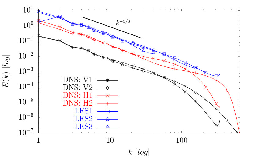
Figure 1: Energy spectra, $E(k)$, averaged on time in the stationary state for the different sets of simulations. The spectra for the LES are shifted upward while the spectra for data-sets with normal viscosity (V) are shifted downward.

4.1 Second-order balance $(n=2)$

Following Ref. [28] and eq. (13) we obtain the equivalent of the four-fifth law within the LES formulation which reads in the stationary state:

$$\frac{1}{r}\left(D^{3,0}(r)+3G^{1,0}_{L,L}(r,\Delta)\right)=-\frac{4}{5}\langle\overline{\Pi}(\Delta)\rangle\ ,$$ (35)

where we have neglected the forcing contribution because it is always sub-leading for scales smaller than the forcing scale $L_{f}$; see Appendix A.1. In Fig. 2(a), we show the importance of the two terms on the left-hand side, using both the filtered DNS data at $12\leqslant k_{c}\leqslant 40$ and the data from the LES1 simulation. Panels (b) and (c) of the same figure show the same curves for LES data only upon changing the resolution. It is clear that the LES approach does not introduce any important spurious physics in the inertial range if compared either with the viscous or the hyperviscous simulations. In particular, panel (a) shows that the LES curves are recovered from the a-priori analysis by decreasing the filter cut-off. The solid lines $(r/\Delta)^{-\zeta_{2}}$ in Figs. 2(a-c) indicate the MF prediction for $G_{L,L}^{1,0}(r,\Delta)/r$, which for $n=1$ and $m=0$ would give $G_{L,L}^{1,0}(r,\Delta)/r\sim r^{\zeta_{3}-\zeta_{2}-1}=r^{-\zeta_{2}}$. It is clear from the figures that $G_{L,L}^{1,0}(r,\Delta)$ does not obey the MF scaling in both the a-priori and the a-posteriori analyses. Instead, interestingly enough, it is even more sub-leading than the MF prediction, indicating that the details of the SGS-model should have little effect on the energy balance. The deviation from the MF in the DNS data is probably due to the existence of cancellations given the particular structure of $G_{L,L}^{1,0}(r,\Delta)$ where the longitudinal increments appear only in a linear way, a fact that would lead to an exactly vanishing contribution in the case of weak correlation with the SGS stress tensor, because of homogeneity. For the LES case we will comment on this later on in this section. Since $D^{3,0}(r)\sim r^{3}$ for $r\to 0$, $G^{1,0}_{L,L}(r,\Delta)$ must satisfy $-3G^{1,0}_{L,L}(r,\Delta)=\frac{4}{5}\langle\Pi(\Delta)\rangle$ for $r\to 0$. This is the case as can be seen in Fig. 2(a)-(c) for both the filtered DNS and the LES. Moreover, the scaling range of the correlation and structure functions obtained though the LES simulations extends with increasing resolution as shown in Figs. 2(b,c), as it must be expected for a good subgrid parametrisation.
Finally, we compare in Fig. 3 the highest resolved LES3 data-set against results from the viscous and hyperviscous data-sets V1 and H1 without filtering, where all simulations were carried out on $1024^{3}$ grid points. Here, for the two data sets from the Navier-Stokes cases we need to consider that the $4/5$ law (35) will include the dissipative term: $\nu\mathcal{L}^{\alpha}_{r}D^{2,0}(r)$, where $\mathcal{L}^{\alpha}_{r}$ is a differential operator which depends on the order $\alpha$ of the Laplacian. The dissipative term replaces term $G^{1,0}$ in the $4/5$-th law; for data-set V1 it is given as $\mathcal{L}^{1}_{r}D^{2,0}(r)/r=6\partial_{r}D^{2,0}(r)/r$ while for data-set H1 $\mathcal{L}^{2}_{r}D^{2,0}(r)/r=12D^{2,0}(r)/r^{2}+12(\int_{0}^{r}ds\ sD^{2,0}(r))/r^{4}-6\partial_{r}^{3}D^{2,0}(r)/r$.

For data-set V1, the form of the dissipative term implies that it should scale as $r^{\zeta_{2}-2}\approx r^{-1.3}$, which is well satisfied, as can be seen from panel (a). Interestingly, the function $G^{1,0}_{L,L}(\Delta,r)/r$ scales similarly as a function of $r$ at fixed $\Delta$; a possible explanation for this behaviour is given below in eq.(36). For data-set H1, $\mathcal{L}^{2}_{r}D^{2,0}(r)/r=12D^{2,0}(r)/r^{2}+12(\int_{0}^{r}ds\ sD^{2,0}(r))/r^{4}-6\partial_{r}^{3}D^{2,0}(r)/r$, and therefore, at leading order $\mathcal{L}^{2}_{r}D^{2,0}(r)/r\sim D^{2,0}(r)/r^{2}$ for $r>\eta_{\alpha}$, does show the same scaling properties as the viscous case. Panel (b) shows that the third-order structure function obtained from LES3 has an inertial-range scaling much more extended than the viscous case and even better than the H1, supporting the statement that the LES closure is a dissipative closure more efficient than hyperviscosity. Overall, we can conclude that if the use of the hyperviscosity is interpreted as an effective ‘subgrid model’, it leads to a larger influence of the dissipative term than the SGS modelling of the LES simulation.

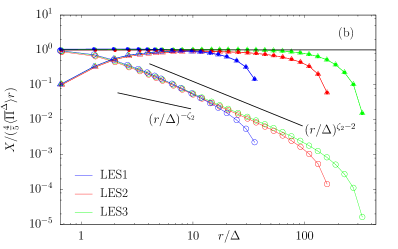
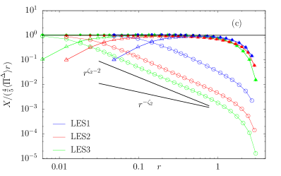
Figure 2: Top panel (a): comparison of the two terms in the left hand side of the four-fifth law, eq. (35). Full symbols represent $D^{3,0}(r)$ while open symbols are $3G^{1,0}(r,\Delta)$, both normalised with $4/5\langle\overline{\Pi}(\Delta)\rangle r$. The two terms are calculated for the LES1 data-set at $\Delta=\pi/42$ (circles) and for the filtered DNS data using different cut-off $\Delta$, (black rhombus) $\Delta=\pi/12$, (black downwards triangles) $\Delta=\pi/20$, (black upwards triangles) $\Delta=\pi/30$ and (black squares) $\Delta=\pi/40$. Bottom panels (b and c): the same quantities, $D^{3,0}(r)$ (full triangles) and $3G^{1,0}(r,\Delta)$ (open circles) are presented for different LES data-sets, namely: LES1, $\Delta=\pi/42$ (blue coluor/dark grey). LES2, $\Delta=\pi/171$ (red/grey) and LES3 $\Delta=\pi/342$ (green/light grey) against $r/\Delta$ in panel (b) and against $r$ in panel (c). The solid line $(r/\Delta)^{-\zeta_{2}}$ shown in all panels, indicates the MF scaling prediction (25), while the solid line $(r/\Delta)^{\zeta_{2}-2}$ corresponds to the scaling prediction based on the assumption of a constant eddy viscosity (36).

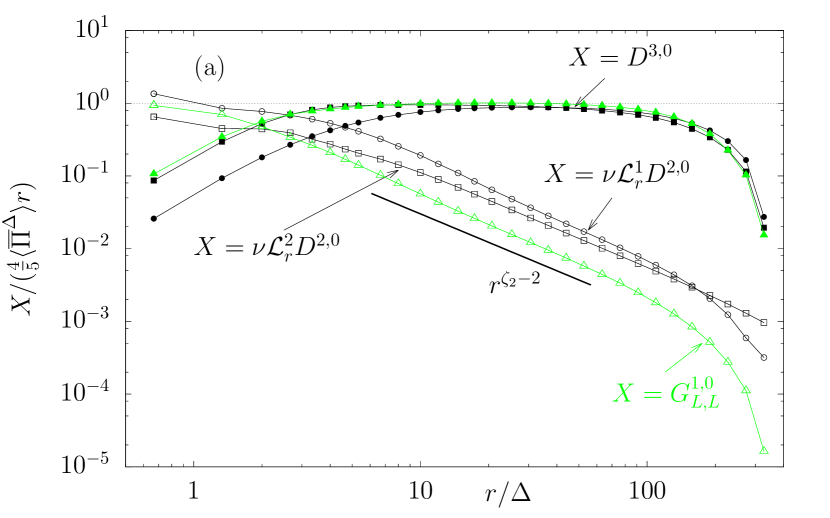
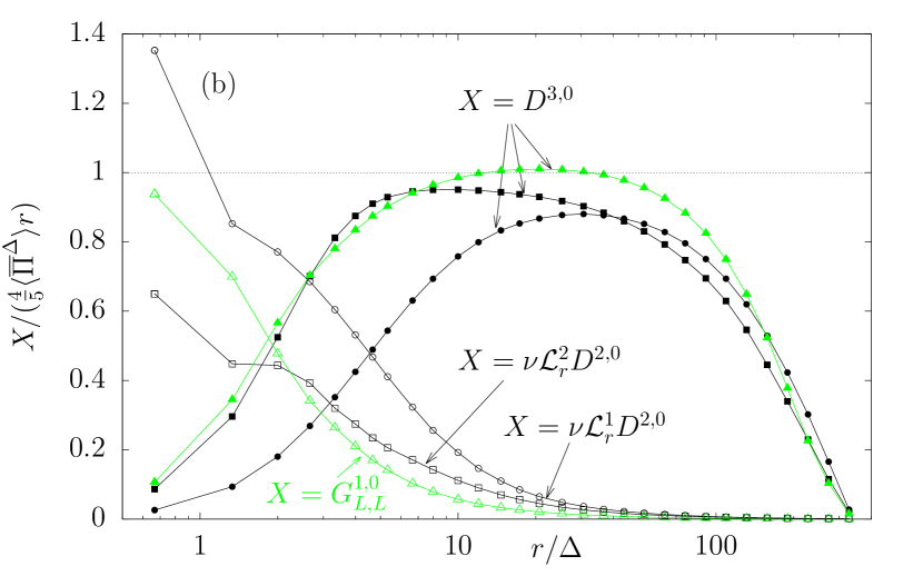
Figure 3: Four-fifth law: comparison between full DNSs’ data with normal viscosity (V1, black circles), with hyperviscosity (H1) (black squares) and the Smagorinsky LES data at $\Delta=\pi/342$ (green/light grey triangles) always using $1024^{3}$ grid points. Full symbols are the third order structure functions $D^{3,0}(r)$ while open symbols represent either the viscous term, $\nu\mathcal{L}^{\alpha}_{r}D^{2,0}_{L,L}(r)$ (black colour), or the correlation with the SGS tensor, $G^{1,0}(r,\Delta)$ (green/light grey). All terms are normalised with $4/5\langle\overline{\Pi}(\Delta)\rangle r$. Panel (a): data are presented in log-log scale to show the scaling properties of the different functions. Panel (b): same data in lin-log scale to highlight how the four-fifth law expected value (dashed line) is recovered by the different structure functions in the inertial range.

Before moving to the balance equation of higher-order correlations, let us have a look in more details at the scaling of the SGS-term in the $4/5$ law, $G^{1,0}_{L,L}(r,\Delta)$. As noticed, we observe a deviation from the MF prediction and a good agreement with the purely dissipative scaling $G^{1,0}_{L,L}(r,\Delta)\sim r^{\zeta_{2}-1}$. This can be understood considering that using the Smagorinsky closure (34), one breaks the phase correlation between the three velocity increments entering in the SGS modelling, due to the fact that two terms appear inside the square-root and have a definite sign. As a result, concerning multi-scale correlation, the SGS Smagorinsky stress will behave as $\tau^{\Delta,SMAG}\sim const\,\bar{s}_{ij}$. If this is the case, one predicts the SGS tensor to act as a linear dissipative operator:

$$G^{n,0}_{L,L}(r,\Delta)\sim\partial_{r}D^{n+1,0}(r)\sim r^{\zeta_{n+1}-1}$$ (36)

explaining the scaling shown in Fig.(3) for $G^{1,0}_{L.L}(r,\Delta)/r\sim r^{\zeta_{2}-2}$.

In summary, the Smagorinsky SGS-model performs well at the level of the second-order balance equation in the sense that:
(1) Both $D^{3,0}(r)$ and $G^{1,0}_{L,L}(r,\Delta)$ obtained from the LES show the same scaling behaviour as those obtained from filtered DNS.
(2) The effect of the SGS-stress on the two-point energy balance is subleading.
(3) The measured scaling of $G^{1,0}_{L,L}(r,\Delta)$ obtained from the Smagorinsky LES is robust under increasing scale separation between $r$ and $\Delta$.
(4) At the same resolution, the LES simulation have a larger extension of the DNS, even if compared with the hyperviscous Navier-Stokes case.

4.2 Higher-order balances $(3\leqslant n\leqslant 6)$

Having examined the properties of correlations between velocity field increments and the SGS-stress at the lowest nontrivial order in the LES structure function hierarchy, we now examine the higher-order balances. Here, we need to study the correlations which involve the resolved velocity field gradients, $T^{n}_{i,j}(r,\Delta)$ and $S^{n}_{i,j}(r,\Delta)$ also. The latter describe the correlations between velocity field increments and part of the SGS energy transfer. As will become clear in the following, even- and odd-order balances require separate descriptions. In Figure 4 top panel we present all terms in Eq. (2) for $n=3$, obtained from the filtered DNS data-set H1 for $k_{c}=40$, while Figure 4 bottom panel presents the same terms for the a-posteriori data-set LES3. The higher-order analysis, $n=4$, $n=5$ and $n=6$, are reported, respectively, in Figures 5-7 where the results from filtered DNS are presented in the left panels and compared to the one from the LES3 data-set shown in the right panels. The forcing term is not shown in order to improve the readability of the individual figures.
Let us comment the general trends.
(i) For all orders, a-priori (DNS) and a-posteriori (LES) data are in pretty good agreement, especially concerning the leading terms. This is seen by noticing that for all orders the inertial range behaviour is dominated by the structure functions, $D^{n,m}(r)$ (black data). Moreover, the scaling is in agreement with the MF prediction (19) and LES data do scale better than DNS data.
(ii) Correlation function involving Pressure (green/light grey data) do scale similarly to $D^{n,m}(r)$, suggesting a key role of them in the global balance.
(iii) For even orders $(n=4,6)$ also the correlation, $S^{n}_{i,j}(r,\Delta)$ involving the SGS-energy transfer (blue/dark grey colour in Fig. 5 and Fig.7 ) play a leading role, in agreement with what was found for the equivalent terms involving the correlation with the energy dissipation in Navier-Stokes case in [57].
(iv) The ensemble of correlation involving the SGS tensor $G^{n,m}(r,\Delta)$, (red/grey data) are always sub-leading and DNS data do show a different scaling from LES data.
(v) Correlation given by the terms, $T^{n}_{i,j}(r,\Delta)$, are never leading with respect to $S^{n}_{i,j}(r,\Delta)$ (both in blue/dark grey colour in all Figures) as argued after Eq. (29).
Let us now comment more on the previous results. We first focus on the analysis of the data from the filtered DNS. As can be seen from a qualitative comparison the odd- and even-order balances show important differences. For the odd orders (Figures 4 and 6), the pressure correlations must balance the inertial Structure Functions contribution, $D^{n,m}(r)$, as all the other terms scale in a sub-leading way. For the even orders (Figures 5 and 7), the inertial terms are balanced also by the terms $S^{n}_{i,j}(r,\Delta)$, which describe the correlations between longitudinal velocity-field increments and the components of the SGS-energy transfer. These differences could have been expected from numerical results concerning the hierarchy of structure functions in the original NSE obtained in [57]. Indeed, similar to the present case of filtered DNS, it was found in [57] that the inertial contributions are balanced by the pressure for the odd-order balances. For the even-order balances, the inertial contributions are balanced also by the contributions from the viscous terms. The latter is similar to our results for filtered DNS, as the correlations between the resolved-scale velocity increments and the SGS energy transfer play a similar role to the viscous energy dissipation in the full Navier-Stokes evolution – with the important difference that energy dissipation is point-wise positive definite in the NSE. Differences between even- and odd-order balances, in the filtered DNS data, are also visible concerning the functions $S^{n}_{i,j}(r,\Delta)$ and $T^{n}_{i,j}(r,\Delta)$. The latter is always decaying by going to larger and large scale separations, $r/\Delta\gg 1$, the former matches the MF prediction (30) only for even order (see right panels of Figs. (5) and (7), while odd orders are much more depleted and very close to $T^{n}_{i,j}(r,\Delta)$ (top panel of Fig. 4 and left panel of Fig. 6). The above behaviour can be understood by noticing that odd-order $S^{n}_{i,j}(r,\Delta)$ correlations involves unsigned velocity increments and SGS energy transfer, introducing non-trivial cancellations that brings the quantity away from its leading MF prediction.
Concerning LES data, we found that $S^{n}_{i,j}(r,\Delta)$ is in good agreement with DNS for even orders (left columns of Figs. (5) and (7), while it is more intense than the a-priori case for odd orders (bottom panel of Fig. 4 and right panel of Fig. 6). This is probably due to the fact that in the Smagorinsky LES the SGS energy transfer is positive definite, and it is not able to reproduce the cancellations present in the real DNS, leading to a contribution larger than what would be in reality.

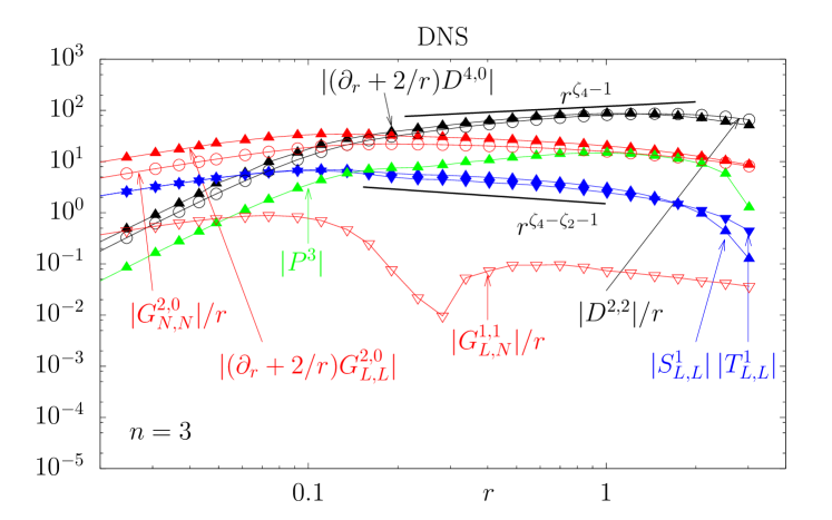
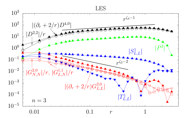
Figure 4: Absolute value of terms contributing to the third-order balance equations, explicitly written in the right-hand side of eq. (2), for filtered DNS at $\Delta=\pi/40$ from data-set H1 (top panel) and for Smagorinsky LES from data-set LES3 (bottom panel).

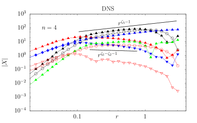
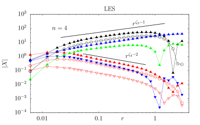
Figure 5: Absolute value of all terms, $|X|$, contributing to the fourth-order balance equations, explicitly written in the right-hand side of eq. (2), for filtered DNS at $\Delta=\pi/40$ from data-set H1 (left panel) and for Smagorinsky LES from data-set LES3 (right panel). Black: $|\left(\partial_{r}+\frac{2}{r}\right)D^{5,0}(r)|$ (solid triangles), $|\left(\frac{8}{r}\right)\ D^{3,2}(r)|$ (circles). Red/grey: $|\left(\partial_{r}+\frac{2}{r}\right)G^{3,0}_{L,L}(r,\Delta)|$ (solid triangles), $|\left(\frac{16}{r}\right)G^{3,0}_{N,N}(r,\Delta)|$ (circles). $|\left(\frac{16}{r}\right)G^{2,1}_{L,N}(r,\Delta)|$ (hollow triangles). Blue/dark grey: $|S^{2}_{L,L}(r,\Delta)|$ (solid up triangles), $|T^{2}_{L,L}(r,\Delta)|$ (solid down triangles). Green/light grey: $|P^{4}(r,\Delta)|$.

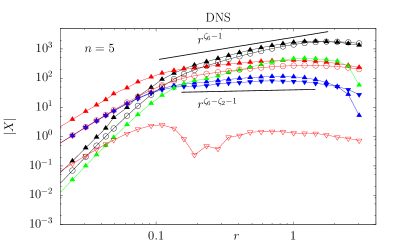
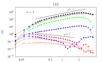
Figure 6: Absolute value of all terms, $|X|$, contributing to the fifth-order balance equations, coming from the right hand side of the hierarchy eq. (2) for $n=5$. (Left panel) data for filtered DNS at $\Delta=\pi/40$ from data-set H1 and (right panel) data for Smagorinsky LES from data-set LES3. Black: $|\left(\partial_{r}+\frac{2}{r}\right)D^{6,0}(r)|$ (solid triangles), $|\left(\frac{10}{r}\right)\ D^{4,2}(r)|$ (circles). Red/grey: $|\left(\partial_{r}+\frac{2}{r}\right)G^{4,0}_{L,L}(r,\Delta)|$ (solid triangles), $|\left(\frac{20}{r}\right)G^{4,0}_{N,N}(r,\Delta)|$ (circles). $|\left(\frac{20}{r}\right)G^{3,1}_{L,N}(r,\Delta)|$ (hollow triangles). Blue/dark grey: $|S^{3}_{L,L}(r,\Delta)|$ (solid up triangles), $|T^{3}_{L,L}(r,\Delta)|$ (solid down triangles). Green/light grey: $|P^{5}(r,\Delta)|$.

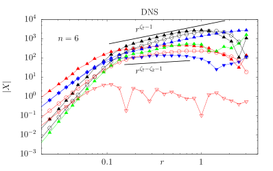
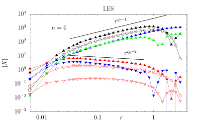
Figure 7: Absolute value of all terms, $|X|$, contributing to the sixth-order balance equations, coming from the right hand side of the hierarchy eq. (2) for $n=6$. (Left panel) data for filtered DNS at $\Delta=\pi/40$ from data-set H1 and (right panel) data for Smagorinsky LES from data-set LES3. Black: $|\left(\partial_{r}+\frac{2}{r}\right)D^{7,0}(r)|$ (solid triangles), $|\left(\frac{12}{r}\right)\ D^{5,2}(r)|$ (circles). Red/grey: $|\left(\partial_{r}+\frac{2}{r}\right)G^{5,0}_{L,L}(r,\Delta)|$ (solid triangles), $|\left(\frac{24}{r}\right)G^{5,0}_{N,N}(r,\Delta)|$ (circles). $|\left(\frac{24}{r}\right)G^{4,1}_{L,N}(r,\Delta)|$ (hollow triangles). Blue/dark grey: $|S^{4}_{L,L}(r,\Delta)|$ (solid up triangles), $|T^{4}_{L,L}(r,\Delta)|$ (solid down triangles). Green/light grey: $|P^{6}(r,\Delta)|$.

To be more quantitative, we show in all figures the straight-line corresponding to scaling MF predictions (30) for the dominant contribution, which is in very good agreement for all cases. The values for the scaling exponents $\zeta_{n}$ of the $n^{\rm th}$-order longitudinal correlation functions used in this comparison are taken from Ref. [7, 12], i.e., $\zeta_{2}=0.70\pm 0.01$, $\zeta_{4}=1.29\pm 0.03$, $\zeta_{5}=1.54\pm 0.03$, $\zeta_{6}=1.77\pm 0.04$ and $\zeta_{7}=1.98\pm 0.06$.
As noticed, the whole set of multi-scale correlation function involving the SGS stress (red data) given by the class $G(r,\Delta)$ are always sub-leading with respect to $D^{n,m}(r)$ and to the pressure and they are in good agreement with the MF prediction (31) for the a-priori DNS data and with (36) for the a-posteriori LES case (as shown by the corresponding straight lines in all plots). Before concluding, let us summarise the main findings.
1. A simple LES approach based on a Smagorinsky model is able to reproduce most of the multi-scale physical properties of real turbulence at high Reynolds numbers, including the MF scaling in the inertial range of the structure functions, $D^{n,m}(r)$, and of the correlation among velocity increments and the SGS energy transfer, $S^{n}(r,\Delta)$ (for even $n$).
2. Nevertheless, some notable differences arise. In particular, the multi-scale correlations (8) involving the SGS stress tensor have a smaller amplitude in LES than for real DNS. By comparing the left and right columns of Figs. (5-7) one clearly sees that for LES data, there exists a sharp difference among those correlations that have the leading scaling behaviour and those that follow off for large $r/\Delta$ separation. This fact is a positive outcome, indicating that the LES closure has a minor influences on the inertial range scaling properties than standard viscosity or hyperviscous effects. A different trend is also measured for the behaviour of correlation, $S^{3}_{ij}(r,\Delta)$, which appears in the balance for $n=5$ in Fig. (6) where the LES data (right panel) do have a better scaling with a larger exponents than the DNS data (left panel).

5 Conclusions

This paper provides analytical and numerical results concerning the multiscale correlations between the resolved-scale velocity field increments and SGS quantities for a-priori and a-posteriori data. We derived the exact hierarchy of higher-order equations for all structure functions obtained from filtered NSE. All correlations were measured using a database consisting of filtered DNS on up to $2048^{3}$ and Smagorinsky LES on up to $1024^{3}$ collocation points.
Under the assumption of a connection between resolved-scale and SGS statistics given by a multiplicative MF cascade process, we provided scaling estimates for all two-point functions involving correlations among the resolved velocity increments and the SGS stress or the SGS energy transfer.
Concerning the comparison between filtered DNS and Smagorinsky LES, we find that the results obtained from the Smagorinsky model agree well with those from filtered DNS concerning all leading terms, i.e. those involving structure functions, pressure correlations and correlations with the SGS-energy transfer. On the contrary, all terms involving correlations with SGS tensor, $G_{i,j}^{n,m}(r,\Delta)$ have a smaller amplitude and a faster decrease as a function of the scale separation $\Delta/r$ for LES data.
Overall, the LES approach works well, leading to a larger extension of the scaling range with respect to the DNS at comparable numerical resolution. Since the Smagorinsky model performs well concerning the scaling of the structure functions, in principle we do not expect significant improvements from more sophisticated models. However, a better LES model may be more efficient in reproducing inertial-range scaling than the Smagorinsky model, in the sense that coarser grids may be possible for a suitable model. A more detailed quantitative assessment of the effects of LES modelling on the inertial range scaling properties, also comparing different subgrid closures will be presented elsewhere.
Moreover, the numerical study of the a-priori filtered DNS data revealed some differences in the scaling behaviour of correlation functions belonging to even- and odd-order balance equations, similar to results concerning the viscous contributions obtained from the full Navier-Stokes evolution [57]. For even-order balances the leading terms are the ones given by velocity structure functions, $D^{n,m}(r)$, the pressure, $P^{n}(r,\Delta)$ and the correlation with the SGS energy transfer, $S^{n}_{i,j}(r,\Delta)$. All of them follow the MF prediction (30). For odd orders, the cross correlation involving the SGS energy balance are subleading. Terms involving the cross correlation with the SGS tensor, $G_{i,j}^{n,m}(r,\Delta)$ are always sub-leading as well, as predicted by the MF; see Eq. (31).
In the Appendices we reproduce all technical aspects concerning the derivation of the exact hierarchy for LES (see Appendix A) and for a modification of the closure equations where we explicitly took into account also the re-projection of the nonlinear term involving the two filtered fields [2, 58, 59, 50] which is somehow unavoidable in numerical applications; see Appendix B. The latter induced complications in the derivation of the structure function hierarchy, which are tackled through a distinction between the actual SGS stress and the Leonard stress [60]. The contributions from the Leonard stress only appear in the higher-order balance equation, with the four-fifth law ($n=2$ in the hierarchy) remaining unaffected (see Appendix B and Ref. [50]). The properties of the correlation tensors, which are used in the derivation of the LES-hierarchy of longitudinal structure functions are summarised in Appendices C.1 and C.2 for those of type $G_{i,j}^{n,m}(r,\Delta)$, $S_{i,j}^{n}(r,\Delta)$ and $T_{i,j}^{n}(r,\Delta)$, where we also comment on the general structure of these terms. The latter is also used in Appendix C.3 in order to provide an explicit form of the pressure correlation, which distinguishes correlations involving velocity-field gradients from those only involving correlations between the pressure and the velocity-field increments. Finally, Appendix A.1 contains a re-derivation of the $4/5$-th law for LES from the tensorial approach, and a subsequent comparison to the corresponding result in Ref. [28]. It is important to stress that studies similar to the one presented here can be performed also in the presence of anisotropy, for wall-bounded [61] and high-Reynolds boundary layer flows [62]. In these cases, the injection of energy due to the coupling with the mean shear leads to an increasing of intermittency and to a more complicated scale-by-scale energy balance [63, 64]. Small-scale vorticity production is the key mechanisms that needs to be captured by LES acting prominently at the cut-off scales [65, 66]. Feedback of intense-but-rare small-scale fluctuations on the resolved large-scale and on the mean profiles is even more important than in homogeneous and isotropic case. An extension of our present study on LES of wall bounded flows, would help to better quantify the accuracy of different sub-grid models for such systems also for higher-orders statistics.

Appendix A Derivation of the LES structure function hierarchies

This appendix contains the derivation of Eq. (2) from Eq. (2). Since all tensors in Eq. (2) which do not contain explicit correlations to the SGS stress are structurally identical to those figuring in the evolution equations derived from the full NSE, the only term that needs to be considered is the tensor

$$H_{i_{1}\ldots i_{n}}=\frac{1}{|S_{n-1}|}\sum_{\sigma\in S_{n}}\langle\delta_{r}\overline{v}_{i_{\sigma(1)}}\ldots\delta_{r}\overline{v}_{i_{\sigma(n-1)}}\delta_{r}(\partial_{k}\tau^{\Delta}_{ki_{\sigma(n)}})\ .$$ (37)

This expression has been obtained through point splitting, that is one considers two points ${\bf x}^{\prime}$ and ${\bf x}$ such that ${\bf x}^{\prime}={\bf x}+{\bf r}$. In order to separate single- and multiscale contributions to the tensor $H$, we carry out a change of variables using

$${\bf X} =\frac{1}{2}({\bf x}+{\bf x}^{\prime})\ \mbox{ and }\ {\bf r}={\bf x}^{\prime}-{\bf x}\ ,$$ (38)

$${\bf x}^{\prime} ={\bf X}+\frac{1}{2}{\bf r}\ \mbox{ and }\ {\bf x}={\bf X}-\frac{1}{2}{\bf r}\ ,$$ (39)

which leads to

$$\partial_{X_{i}} =\partial_{x_{i}^{\prime}}+\partial_{x_{i}}\ ,$$ (40)

$$\partial_{r_{i}} =\frac{1}{2}(\partial_{x_{i}^{\prime}}-\partial_{x_{i}})\ ,$$ (41)

$$\partial_{x_{i}^{\prime}} =\frac{1}{2}\partial_{X_{i}}+\partial_{r_{i}}\ ,$$ (42)

$$\partial_{x_{i}} =\frac{1}{2}\partial_{X_{i}}-\partial_{r_{i}}\ .$$ (43)

In the new coordinates the increment $\delta_{r}(\partial_{k}\tau^{\Delta}_{ki})$ can be written as

$$\delta_{r}(\partial_{k}\tau^{\Delta}_{ki})=\partial_{x_{k}^{\prime}}\tau^{\Delta\prime}_{ki}-\partial_{x_{k}}\tau^{\Delta}_{ki}=(\partial_{x_{k}^{\prime}}-\partial_{x_{k}})(\tau^{\Delta\prime}_{ki}+\tau^{\Delta}_{ki})=2\partial_{r_{k}}(\tau^{\Delta\prime}_{ki}+\tau^{\Delta}_{ki})\ .$$ (44)

Substitution of this equation into the expression for $H_{i_{1}\ldots i_{n}}$ in eq. (37) yields

$$H_{i_{1}\ldots i_{n}} =\frac{1}{|S_{n-1}|}\sum_{\sigma\in S_{n}}\langle\delta_{r}\overline{v}_{i_{\sigma(1)}}\ldots\delta_{r}\overline{v}_{i_{\sigma(n-1)}}\delta_{r}(\partial_{k}\tau^{\Delta}_{ki_{\sigma(n)}})\rangle$$

$$=\frac{2}{|S_{n-1}|}\sum_{\sigma\in S_{n}}\langle\delta_{r}\overline{v}_{i_{\sigma(1)}}\ldots\delta_{r}\overline{v}_{i_{\sigma(n-1)}}\partial_{r_{k}}(\tau^{\Delta\prime}_{ki_{\sigma(n)}}+\tau^{\Delta}_{ki_{\sigma(n)}})\rangle$$

$$=\frac{2}{|S_{n-1}|}\sum_{\sigma\in S_{n}}\partial_{r_{k}}\langle\delta_{r}\overline{v}_{i_{\sigma(1)}}\ldots\delta_{r}\overline{v}_{i_{\sigma(n-1)}}(\tau^{\Delta\prime}_{ki_{\sigma(n)}}+\tau^{\Delta}_{ki_{\sigma(n)}})\rangle$$

$$-\frac{2}{|S_{n-1}||S_{n-2}|}\sum_{s\in S_{n-1}}\sum_{\sigma\in S_{n}}\langle\delta_{r}\overline{v}_{i_{s(\sigma(1))}}\ldots\delta_{r}\overline{v}_{i_{s(\sigma(n-2))}}\partial_{r_{k}}(\delta_{r}\overline{v}_{i_{s(\sigma(n-1))}})(\tau^{\Delta\prime}_{ki_{\sigma(n)}}+\tau^{\Delta}_{ki_{\sigma(n)}})\rangle\ .$$ (45)

The summands in the last term on the RHS of this equation can also be written as

$$\langle\delta_{r}\overline{v}_{i_{s(\sigma(1))}}\ldots\delta_{r}\overline{v}_{i_{s(\sigma(n-2))}}\partial_{r_{k}}(\delta_{r}\overline{v}_{i_{s(\sigma(n-1))}})(\tau^{\Delta\prime}_{ki_{\sigma(n)}}+\tau^{\Delta}_{ki_{\sigma(n)}})\rangle$$

$$\ \ =\frac{1}{2}\langle\delta_{r}\overline{v}_{i_{s(\sigma(1))}}\ldots\delta_{r}\overline{v}_{i_{s(\sigma(n-2))}}(\partial_{x_{k}^{\prime}}\overline{v}_{i_{s(\sigma(n-1))}}^{\prime}+\partial_{x_{k}}\overline{v}_{i_{s(\sigma(n-1))}})(\tau^{\Delta\prime}_{ki_{\sigma(n)}}+\tau^{\Delta}_{ki_{\sigma(n)}})\rangle\ ,$$ (46)

such that

$$H_{i_{1}\ldots i_{n}} =\frac{2}{|S_{n-1}|}\sum_{\sigma\in S_{n}}\partial_{r_{k}}\langle\delta_{r}\overline{v}_{i_{\sigma(1)}}\ldots\delta_{r}\overline{v}_{i_{\sigma(n-1)}}(\tau^{\Delta\prime}_{ki_{\sigma(n)}}+\tau^{\Delta}_{ki_{\sigma(n)}})\rangle$$

$$\ \ -\frac{1}{|S_{n-1}||S_{n-2}|}\sum_{s\in S_{n-1}}\sum_{\sigma\in S_{n}}$$

$$\qquad\langle\delta_{r}\overline{v}_{i_{s(\sigma(1))}}\ldots\delta_{r}\overline{v}_{i_{s(\sigma(n-2))}}(\partial_{x_{k}^{\prime}}\overline{v}_{i_{s(\sigma(n-1))}}^{\prime}+\partial_{x_{k}}\overline{v}_{i_{s(\sigma(n-1))}})(\tau^{\Delta\prime}_{ki_{\sigma(n)}}+\tau^{\Delta}_{ki_{\sigma(n)}})\rangle$$

$$=\frac{2}{|S_{n-1}|}\sum_{\sigma\in S_{n}}\partial_{r_{k}}\langle\delta_{r}\overline{v}_{i_{\sigma(1)}}\ldots\delta_{r}\overline{v}_{i_{\sigma(n-1)}}(\tau^{\Delta\prime}_{ki_{\sigma(n)}}+\tau^{\Delta}_{ki_{\sigma(n)}})\rangle$$

$$\ \ -\frac{1}{|S_{n-1}||S_{n-2}|}\sum_{s\in S_{n-1}}\sum_{\sigma\in S_{n}}$$

$$\qquad\langle\delta_{r}\overline{v}_{i_{s(\sigma(1))}}\ldots\delta_{r}\overline{v}_{i_{s(\sigma(n-2))}}(\partial_{x_{k}^{\prime}}\overline{v}_{i_{s(\sigma(n-1))}}^{\prime}\tau^{\Delta\prime}_{ki_{\sigma(n)}}+\partial_{x_{k}}\overline{v}_{i_{s(\sigma(n-1))}}\tau^{\Delta}_{ki_{\sigma(n)}})\rangle$$

$$\ \ -\frac{1}{|S_{n-1}||S_{n-2}|}\sum_{s\in S_{n-1}}\sum_{\sigma\in S_{n}}$$

$$\qquad\langle\delta_{r}\overline{v}_{i_{s(\sigma(1))}}\ldots\delta_{r}\overline{v}_{i_{s(\sigma(n-2))}}(\partial_{x_{k}^{\prime}}(\overline{v}_{i_{s(\sigma(n-1))}}^{\prime}\tau^{\Delta}_{ki_{\sigma(n)}})+\partial_{x_{k}}(\overline{v}_{i_{s(\sigma(n-1))}}\tau^{\Delta\prime}_{ki_{\sigma(n)}})\rangle\ ,$$ (47)

and we have separated three contributions; the first term on the RHS describes the correlation between the velocity field increments and the SGS tensor, while the second term describes the correlations between the velocity field increments with the velocity field gradients and the SGS tensor evaluated at the same point and the third term describes the correlations between the velocity field increments with the field gradients and the SGS tensor evaluated at different points. For $n=2$ the second term becomes the subgrid energy flux. We define three tensors to keep track of the different correlations

$$G_{i_{1}\ldots i_{n}k}(r,\Delta) =\langle\delta_{r}\overline{v}_{i_{1}}\ldots\delta_{r}\overline{v}_{i_{n-1}}(\tau^{\Delta\prime}_{i_{n}k}+\tau^{\Delta}_{i_{n}k})\rangle\ ,$$ (48)

$$S_{i_{1}\ldots i_{n}}(r,\Delta) \equiv\langle\delta_{r}\overline{v}_{i_{1}}\ldots\delta_{r}\overline{v}_{i_{n-2}}(\partial_{x_{k}^{\prime}}\overline{v}_{i_{n-1}}^{\prime}\tau^{\Delta\prime}_{i_{n}k}+\partial_{x_{k}}\overline{v}_{i_{n-1}}\tau^{\Delta}_{i_{n}k})\rangle\ ,$$ (49)

$$T_{i_{1}\ldots i_{n}}(r,\Delta) \equiv\langle\delta_{r}\overline{v}_{i_{1}}\ldots\delta_{r}\overline{v}_{i_{n-2}}(\partial_{x_{k}^{\prime}}\overline{v}_{i_{n-1}}^{\prime}\tau^{\Delta}_{i_{n}k}+\partial_{x_{k}^{\prime}}\overline{v}_{i_{n-1}}^{\prime}\tau^{\Delta}_{i_{n}k})\rangle\ ,$$ (50)

and introduce their symmetrised versions

$$G_{\{i_{1}\ldots i_{n}\}k}(r,\Delta) \equiv\frac{1}{|S_{n-1}|}\sum_{\sigma\in S_{n}}G_{i_{\sigma(1)}\ldots i_{\sigma(n)}k}(r,\Delta)\ ,$$ (51)

$$S_{\{i_{1}\ldots i_{n}\}}(r,\Delta) \equiv\frac{1}{|S_{n-1}||S_{n-2}|}\sum_{s\in S_{n-1}}\sum_{\sigma\in S_{n}}S_{i_{s(\sigma(1))}\ldots i_{s(\sigma(n-1))i_{\sigma(n)}}}(r,\Delta)\ ,$$ (52)

$$T_{\{i_{1}\ldots i_{n}\}}(r,\Delta) \equiv\frac{1}{|S_{n-1}||S_{n-2}|}\sum_{s\in S_{n-1}}\sum_{\sigma\in S_{n}}T_{i_{s(\sigma(1))}\ldots i_{s(\sigma(n-1))i_{\sigma(n)}}}(r,\Delta)\ .$$ (53)

We can therefore express the tensor $H_{i_{1}\ldots i_{n}}$ as follows

$$H_{i_{1}\ldots i_{n}}=2\partial_{r_{k}}G_{\{i_{1}\ldots i_{n}\}k}-S_{\{i_{1}\ldots i_{n}\}}-T_{\{i_{1}\ldots i_{n}\}}\ .$$ (54)

From their definitions, it is clear that $S_{\{i_{1}\ldots i_{n}\}}$ and $T_{\{i_{1}\ldots i_{n}\}}$ are isotropic tensors which are symmetric under the exchange of any pair of indices, the same applies to $\partial_{r_{k}}G_{\{i_{1}\ldots i_{n}\}k}$. Therefore $H_{i_{1}\ldots i_{n}}$ is an isotropic tensor which is symmetric under the exchange of any two indices, as it must be. Hence eq. (2) can be written more concisely as

$$\partial_{t}\langle\delta_{r}\overline{v}_{i_{1}}\ldots\delta_{r}\overline{v}_{i_{n}}\rangle= -\partial_{r_{k}}\langle\delta_{r}\overline{v}_{i_{1}}\ldots\delta_{r}\overline{v}_{i_{n}}\delta_{r}\overline{v}_{k}\rangle-P_{\{i_{1}\ldots i_{n}\}}$$

$$-2\partial_{r_{k}}G_{\{i_{1}\ldots i_{n}\}k}(r,\Delta)+S_{\{i_{1}\ldots i_{n}\}}(r,\Delta)+T_{\{i_{1}\ldots i_{n}\}}(r,\Delta)+F_{\{i_{1}\ldots i_{n}\}}\ ,$$ (55)

where $P_{\{i_{1}\ldots i_{n}\}}$ denotes the correlation tensor between the velocity and pressure gradient increments and $F_{\{i_{1}\ldots i_{n}\}}$ the correlation with the force increments. Note that the pressure tensor is structurally similar to $H_{i_{1}\ldots i_{n}}$; therefore, a similar splitting should be possible (see also Ref. [67]) and may be interesting in order to extend the results of Ref. [30] by inclusion of the pressure-velocity correlation functions in explicit form.

The divergence of arbitrary $n^{th}$-order isotropic tensors which are symmetric under the exchange of two indices was calculated in general in Ref. [30] with details given in Ref. [67]. These results can now be applied here, leading to the following hierarchy of equations for the $n$-th order longitudinal structure function $D^{n,0}$:

$$\partial_{t}D^{n,0}(r)= -\left(\partial_{r}D^{n+1,0}(r)+\frac{2}{r}D^{n+1,0}(r)-\frac{2n}{r}D^{n-1,2}(r)\right)$$

$$-2n\left(\partial_{r}+\frac{2}{r}\right)G^{n-1,0}_{L,L}(r,\Delta)+\frac{4n}{r}(G^{n-2,1}_{L,N}(r,\Delta)+G^{n-1,0}_{N,N}(r,\Delta))$$

$$+\frac{2n!}{(n-2)!}(S^{n-2}_{L,L}(r,\Delta)+T^{n-2}_{L,L}(r,\Delta))-2nP^{n}(r,\Delta)+2nF^{n}(r)\ ,$$ (56)

where the usual choice ${\bf r}=(r,0,0)$ was used and the divergence of the $G$-tensors has been evaluated, leading to the presence of the functions $G^{n-1,0}_{L,L}(r,\Delta)$, $G^{n-2,1}_{L,N}(r,\Delta)$ and $G^{n-1,0}_{N,N}(r,\Delta)$. The function $F^{n}$ denotes the contribution from the forcing

$$F^{n}=\langle\underbrace{\delta_{r}\overline{v}_{L}\ldots\delta_{r}\overline{v}_{L}}_{\text{n-1 times}}\delta_{r}f_{L}\rangle\ .$$ (57)

In order to derive this final hierarchy of equations, the tensors $S$ and $T$ and the divergence of the tensors $G$ must be evaluated. Unlike the tensors involving only velocity increments, the tensors $G$ are in general not symmetric with respect to the exchange of arbitrary pairs of indices, which precludes the direct application of results from Ref. [30]. Details of the evaluation of $\partial_{r_{k}}G_{\{i_{1}\ldots i_{n}\}k}$ can be found in Appendix C.1, and the evaluation of the tensors of type $S$ and $T$ is carried out in appendix C.2. The pressure tensors are considered in appendix C.3.

A.1 Recovery of the four-fifth law for LES for $n=2$

We now treat the longitudinal components of $S_{\{ij\}}$, $T_{\{ij\}}$ and $(\partial_{r_{k}}G_{\{ij\}k})$ on the RHS of the tensor equation for the longitudinal case more in detail in order to relate eq. (13) to the corresponding result in Ref. [28]. We begin by evaluating $(\partial_{r_{k}}G_{\{ij\}k})$. From the definition of the third-order tensor

$$G_{\{ij\}k}=\langle\delta_{r}\overline{v}_{i}(\tau^{\Delta\prime}_{jk}+\tau^{\Delta}_{jk})\rangle+\langle\delta_{r}\overline{v}_{j}(\tau^{\Delta\prime}_{ki}+\tau^{\Delta}_{ki})\rangle\ ,$$ (58)

we obtain

$$G_{\{ij\}k} =2\left[\langle\overline{v}_{i}^{\prime}\tau^{\Delta}_{jk})\rangle+\langle\overline{v}_{j}^{\prime}\tau^{\Delta}_{ki}\rangle\right]\ ,$$ (59)

since $\langle\overline{v}_{i}\tau^{\Delta\prime}_{jk}\rangle=-\langle\overline{v}_{i}^{\prime}\tau^{\Delta}_{jk}\rangle$ (see Appendix C.1). The evaluation of the divergence of $G_{\{ij\}k}$ can be simplified through the incompressibility constraint, which results in $\partial_{r_{k}}\langle\overline{v}_{k}^{\prime}\tau^{\Delta}_{ij}\rangle=0$. Therefore one obtains

$$\partial_{r_{k}}G_{\{ijk\}}(r,\Delta) =2\partial_{r_{k}}\langle\overline{v}_{i}^{\prime}\tau^{\Delta}_{jk}+\overline{v}_{j}^{\prime}\tau^{\Delta}_{ik}+\overline{v}_{k}^{\prime}\tau^{\Delta}_{ij}\rangle$$

$$=2\partial_{r_{k}}\langle\overline{v}_{i}^{\prime}\tau^{\Delta}_{jk}+\overline{v}_{j}^{\prime}\tau^{\Delta}_{ik}\rangle=\partial_{k}G_{\{ij\}k}\ ,$$ (60)

where the tensor $G_{\{ijk\}}=G_{\{ij\}k}+\langle\delta_{r}\overline{v}_{k}(\tau^{\Delta\prime}_{ij}+\tau^{\Delta}_{ij})\rangle$ is an isotropic tensor which is symmetric under exchange of any pair of indices. Alongside incompressibility, these geometric constraints result in $G_{\{ijk\}}$ to be of the following form [68, 51]

$$G_{\{ijk\}}=(G^{1,0}_{L,L}-r\partial_{r}G^{1,0}_{L,L})\frac{3r_{i}r_{j}r_{k}}{2r^{3}}+(G^{1,0}_{L,L}+r\partial_{r}G^{1,0}_{L,L})\left[\frac{r_{i}}{2r}\delta_{jk}+\frac{r_{j}}{2r}\delta_{ki}+\frac{r_{k}}{2r}\delta_{ij}\right]\ ,$$ (61)

and its divergence can be calculated using the general results on the divergence of an isotropic tensor which is symmetric under exchange of any pair of indices (see Ref. [30])

$$\partial_{r_{k}}G_{\{ijk\}} =\left[\left(\partial_{r}+\frac{2}{r}\right)\left(\frac{3(G^{1,0}_{L,L}-r\partial_{r}G^{1,0}_{L,L})}{2}\right)+\left(2\partial_{r}-\frac{2}{r}\right)\left(\frac{G^{1,0}_{L,L}+r\partial_{r}G^{1,0}_{L,L}}{2}\right)\right]\frac{r_{i}r_{j}}{r^{2}}$$

$$\ \ +\left[\left(\partial_{r}+\frac{4}{r}\right)\left(\frac{G^{1,0}_{L,L}+r\partial_{r}G^{1,0}_{L,L}}{2}\right)\right]\delta_{ij}\ .$$ (62)

The evaluation of the tensor $S_{\{ij\}}$ is straightforward

$$S_{\{ij\}} =\langle(\partial_{x^{\prime}_{k}}\overline{v}_{i}^{\prime})\tau^{\Delta\prime}_{jk}+(\partial_{x_{k}}\overline{v}_{i})\tau^{\Delta}_{jk}+(\partial_{x^{\prime}_{k}}\overline{v}_{j}^{\prime})\tau^{\Delta\prime}_{ki}+(\partial_{x_{k}}\overline{v}_{j})\tau^{\Delta}_{ki}\rangle$$

$$=2\langle(\partial_{x_{k}}\overline{v}_{i})\tau^{\Delta}_{jk}+(\partial_{x_{k}}\overline{v}_{j})\tau^{\Delta}_{ik}\rangle\ .$$ (63)

Owing to the incompressibility constraint, the tensor $T_{\{ij\}}$ can in fact be expressed in terms of the divergence of $G$

$$T_{\{ij\}} =\langle(\partial_{x^{\prime}_{k}}\overline{v}_{i}^{\prime}+\partial_{x_{k}}\overline{v}_{i})(\tau^{\Delta\prime}_{jk}+\tau^{\Delta}_{jk})\rangle+\langle(\partial_{x^{\prime}_{k}}\overline{v}_{j}^{\prime}+\partial_{x_{k}}\overline{v}_{j})(\tau^{\Delta\prime}_{ki}+\tau^{\Delta}_{ki})\rangle$$

$$=\langle\partial_{x_{k}}(\overline{v}_{i}\tau^{\Delta\prime}_{jk})+\partial_{x^{\prime}_{k}}(\overline{v}_{i}^{\prime}\tau^{\Delta}_{jk})\rangle+\langle\partial_{x_{k}}(\overline{v}_{j}\tau^{\Delta\prime}_{ik})+\partial_{x^{\prime}_{k}}(\overline{v}_{j}^{\prime}\tau^{\Delta}_{ik})\rangle$$

$$=2\partial_{r_{k}}\langle\overline{v}_{i}^{\prime}\tau^{\Delta}_{jk}+\overline{v}_{j}^{\prime}\tau^{\Delta}_{ik}\rangle=\partial_{r_{k}}G_{\{ijk\}}(r,\Delta)\ ,$$ (64)

where the last equality follows from incompressibility: $\partial_{r_{k}}\langle\overline{v}_{k}^{\prime}\tau^{\Delta}_{ij}\rangle=0$. The longitudinal components of three tensors then become

$$\left(\partial_{r_{k}}G_{\{ijk\}}(r,\Delta)\right)_{LL} =2\frac{\partial_{r}}{r^{4}}(r^{4}G^{1,0}_{L,L}(r,\Delta))=\frac{\partial_{r}}{r^{4}}(r^{4}G_{LLL}(r,\Delta))\ ,$$ (65)

$$S^{2}_{L,L} =\langle\tau^{\Delta}_{kL}\partial_{x_{k}}\overline{v}_{L}\rangle\ ,$$ (66)

$$T^{2}_{L,L}(r,\Delta) =\frac{1}{4}\left(\partial_{r_{k}}G_{\{ijk\}}(r,\Delta)\right)_{LL}=\frac{\partial_{r}}{4r^{4}}(r^{4}G^{1,0}_{L,L}(r,\Delta))\ ,$$ (67)

and we obtain

$$\partial_{t}D^{2,0}=-\frac{\partial_{r}}{3r^{4}}(r^{4}D^{3,0})-2\frac{\partial_{r}}{r^{4}}(r^{4}G^{1,0}_{L,L})+4S^{2}+\frac{\partial_{r}}{r^{4}}(r^{4}G^{1,0}_{L,L})+2F^{2}\ ,$$ (69)

from which for $\partial_{t}D^{2,0}=0$ and $F^{2}=0$ we recover eq. (47) in Ref. [28] stated here in the notation used in Ref. [28]

$$D_{LLL}=-6G_{L,LL}(r,\Delta)+\frac{12}{5}\langle\tau^{\Delta}_{kL}\partial_{x_{k}}\overline{v}_{L}\rangle r=-6G_{L,LL}(r,\Delta)+6\langle\tau^{\Delta}_{LL}s_{LL}\rangle r\ .$$ (70)

where

$$G_{LLL}(r,\Delta)=\langle\overline{v}_{L}^{\prime}\tau^{\Delta}_{LL}\rangle=\frac{1}{2}\langle\delta_{r}\overline{v}_{L}(\tau^{\Delta\prime}_{LL}+\tau^{\Delta}_{LL})\rangle=\frac{1}{2}G^{1,0}_{L,L}(r,\Delta)\ ,$$ (71)

and $D_{LLL}\equiv D^{3,0}$. Concerning the last equality in Eq. (70), note that the term $6\langle\tau^{\Delta}_{LL}s_{LL}\rangle$ must equal the SGS energy flux in stationary state, which implies $6\langle\tau^{\Delta}_{LL}s_{LL}\rangle=-\frac{4}{5}\langle\Pi(\Delta)\rangle=\frac{4}{5}\langle\tau^{\Delta}_{kj}s_{kj}\rangle$, which implies $\langle\tau^{\Delta}_{LL}s_{LL}\rangle=\frac{2}{15}\langle\tau^{\Delta}_{kj}s_{kj}\rangle$ (see also eq.  (71) [28]). These relations also imply $\langle\tau^{\Delta}_{kL}\partial_{x_{k}}\overline{v}_{L}\rangle=\langle\tau^{\Delta}_{kj}s_{kj}\rangle/3$. The contribution from the forcing gives

$$2F^{2}=2\langle\delta_{r}\overline{v}_{L}\delta_{r}f_{L}\rangle=\frac{4}{3}\varepsilon_{\rm IN}-4\langle\overline{v}_{L}^{\prime}f_{L}\rangle\ ,$$ (72)

and for $r<<L_{f}$ we can approximate $\langle\overline{v}_{L}^{\prime}f_{L}\rangle\simeq\varepsilon_{\rm IN}/3$ (by isotropy $\langle\overline{v}_{L}f_{L}\rangle=\varepsilon_{\rm IN}/3$). Hence in stationary state, where $\langle\Pi\rangle=\varepsilon_{\rm IN}$, we again recover the four-fifth law with $\langle\Pi\rangle$ replaced by the numerically equal $\varepsilon_{\rm IN}$.

Appendix B Projected LES

In LES applications, the coarse computational grid cannot resolve small-scale dynamics generated by the coupling of resolved-scale velocity-field components. In formal terms, the existence of the LES grid therefore requires the evolution of the resolved-scale velocity field to be confined to the same finite-dimensional vector space; hence, it is necessary to project the momentum equation again, resulting in

$$\partial_{t}\overline{v}_{i}+\partial_{j}(\overline{\overline{v}_{i}\overline{v}_{j}}+\overline{P}\delta_{ij}+\tau^{\Delta,P}_{ij})=f_{i}\ .$$ (73)

The equation derived from this momentum balance at points ${\bf x}$ and ${\bf x}^{\prime}$ for the $n^{th}$-order tensor of velocity-field increments in homogeneous isotropic turbulence then reads

$$\partial_{t}\langle\delta_{r}\overline{v}_{i_{1}}\ldots\delta_{r}\overline{v}_{i_{n}}\rangle= -\frac{1}{|S_{n-1}|}\sum_{\sigma\in S_{n}}$$

$$\left\langle\delta_{r}\overline{v}_{i_{\sigma(1)}}\ldots\delta_{r}\overline{v}_{i_{\sigma(n-1)}}\left[\overline{\left(\frac{\overline{v}_{k}^{\prime}+\overline{v}_{k}}{2}\right)\partial_{X_{k}}\delta_{r}\overline{v}_{i_{\sigma(n)}}}+\overline{\delta_{r}\overline{v}_{k}\partial_{r_{k}}\delta_{r}\overline{v}_{i_{\sigma(n)}}}\right]\right\rangle$$

$$-\frac{1}{|S_{n-1}|}\sum_{\sigma\in S_{n}}\langle\delta_{r}\overline{v}_{i_{\sigma(1)}}\ldots\delta_{r}\overline{v}_{i_{\sigma(n-1)}}\delta_{r}(\partial_{k}\overline{P}\delta_{ki_{\sigma(n)}})\rangle$$

$$-\frac{1}{|S_{n-1}|}\sum_{\sigma\in S_{n}}\langle\delta_{r}\overline{v}_{i_{\sigma(1)}}\ldots\delta_{r}\overline{v}_{i_{\sigma(n-1)}}\delta_{r}(\partial_{k}\tau^{\Delta,P}_{ki_{\sigma(n)}})\rangle$$

$$+\frac{1}{|S_{n-1}|}\sum_{\sigma\in S_{n}}\langle\delta_{r}\overline{v}_{i_{\sigma(1)}}\ldots\delta_{r}\overline{v}_{i_{\sigma(n-1)}}\delta_{r}f_{i_{\sigma(n)}}\rangle\ ,$$ (74)

where

$$\tau^{\Delta,P}_{ij}\equiv\overline{v_{i}v_{j}}-\overline{\overline{v}_{i}\overline{v}_{j}}\ .$$ (75)

A further advantage of the projected LES formulation is that $\tau^{\Delta,P}_{ij}$ only consists of SGS quantities while the unprojected SGS stress $\tau^{\Delta}_{ij}$ includes a residual coupling amongst resolved scales. A detailed discussion of the difference between the two formulations is given in Refs. [59, 58, 50]. For the derivation of a hierarchy of equations for the structure functions from Eq. (B) we immediately run into several difficulties:

1. The correlation tensor of the velocity field increments which arises from the nonlinear term in eq. (73) is no longer symmetric under the exchange of any two indices.

2. Due to the asymmetry caused by the additional projector acting on the nonlinear term, the derivatives with respect to $X_{k}$ cannot be removed by homogeneity, because they cannot be brought out from inside the average.

3. If we wish to bring the derivatives with respect to $r_{k}$ out from inside the average additional terms appear from the product rule of differentiation again due the asymmetry introduced by the projector acting on the nonlinear term.

4. We cannot relate the higher-order structure functions ($n\geqslant 3$, see below) to each other without the introduction of a correction term.

However, by introducing a correction term

$$\tau^{\Delta,LEO}_{ij}\equiv\overline{\overline{v}_{i}\overline{v}_{j}}-\overline{v}_{i}\overline{v}_{j}\ ,$$ (76)

which is known as the Leonard stress [60], it is possible to rewrite the momentum balance (73) as

$$\partial_{t}\overline{v}_{i}+\partial_{j}(\overline{v}_{i}\overline{v}_{j}+\overline{P}\delta_{ij}+\tau^{\Delta,P}_{ij}+\tau^{\Delta,LEO}_{ij})=f_{i}\ .$$ (77)

Using the correction terms originating from the Leonard stress, we obtain for the evolution of the $n^{th}$-order correlation tensor of velocity-field increments

$$\partial_{t}\langle\delta_{r}\overline{v}_{i_{1}}\ldots\delta_{r}\overline{v}_{i_{n}}\rangle= -\partial_{r_{k}}\langle\delta_{r}\overline{v}_{i_{1}}\ldots\delta_{r}\overline{v}_{i_{n}}\delta_{r}\overline{v}_{k}\rangle$$

$$-\frac{1}{|S_{n-1}|}\sum_{\sigma\in S_{n}}\langle\delta_{r}\overline{v}_{i_{\sigma(1)}}\ldots\delta_{r}\overline{v}_{i_{\sigma(n-1)}}\delta_{r}(\partial_{k}\overline{P}\delta_{ki_{\sigma(n)}})\rangle$$

$$-\frac{1}{|S_{n-1}|}\sum_{\sigma\in S_{n}}\langle\delta_{r}\overline{v}_{i_{\sigma(1)}}\ldots\delta_{r}\overline{v}_{i_{\sigma(n-1)}}\delta_{r}(\partial_{k}\tau^{\Delta,P}_{ki_{\sigma(n)}})\rangle$$

$$-\frac{1}{|S_{n-1}|}\sum_{\sigma\in S_{n}}\langle\delta_{r}\overline{v}_{i_{\sigma(1)}}\ldots\delta_{r}\overline{v}_{i_{\sigma(n-1)}}\delta_{r}(\partial_{k}\tau^{\Delta,LEO}_{ki_{\sigma(n)}})\rangle$$

$$+\frac{1}{|S_{n-1}|}\sum_{\sigma\in S_{n}}\langle\delta_{r}\overline{v}_{i_{\sigma(1)}}\ldots\delta_{r}\overline{v}_{i_{\sigma(n-1)}}\delta_{r}f_{i_{\sigma(n)}}\rangle\ ,$$ (78)

where the tensors involving $\tau^{\Delta,P}_{ij}$ and $\tau^{\Delta,LEO}_{ij}$ have the same symmetries. Hence, we can use the results from the derivation of the equation hierarchy following Eq. (2) to deduce the corresponding hierarchy for the projected LES (P-LES) following Eq. (B)

$$\partial_{t}D^{n,0} =-\left(\partial_{r}+\frac{2}{r}\right)(D^{n+1,0}+2n(G^{n-1,0,\rm P}_{L,L}+G^{n-1,0,\rm LEO}_{L,L}))$$

$$\qquad+\frac{2n}{r}(D^{n-1,2}+2(G^{n-2,1,\rm P}_{L,N}+G^{n-1,0,\rm P}_{N,N}+G^{n-2,1,\rm LEO}_{L,N}+G^{n-1,0,\rm LEO}_{N,N}))$$

$$\qquad+\frac{2n!}{(n-2)!}\left(S^{n-2,\rm P}_{L,L}+S^{n-2,\rm LEO}_{L,L}+T^{n-2,\rm P}_{L,L}+T^{n-2,\rm LEO}_{L,L}\right)-2nP^{n}+2nF^{n}\ .$$ (79)

Note that no correction terms are present for $n=2$ since

$$G^{\rm LEO}_{ijk} =2\langle\overline{v}_{i}^{\prime}\tau^{\Delta,\rm LEO}_{jk}\rangle=2\langle\overline{v}_{i}^{\prime}\overline{\overline{v}_{j}\overline{v}_{k}}\rangle-2\langle\overline{v}_{i}^{\prime}\overline{v}_{j}\overline{v}_{k}\rangle=2\langle\overline{v}_{i}^{\prime}\overline{v}_{j}\overline{v}_{k}\rangle-2\langle\overline{v}_{i}^{\prime}\overline{v}_{j}\overline{v}_{k}\rangle=0\ ,$$

$$T^{0,\rm LEO}_{L,L} =\frac{1}{4}\left(\partial_{r_{k}}G^{\rm LEO}_{ijk}\right)_{LL}=0\ ,$$

$$S^{0,\rm LEO}_{L,L} =\langle\tau^{\Delta,\rm LEO}_{kL}\partial_{x_{k}}\overline{v}_{L}\rangle=\langle(\overline{\overline{v}_{k}\overline{v}_{L}}-\overline{v}_{k}\overline{v}_{L})\partial_{x_{k}}\overline{v}_{L}\rangle=\langle\overline{\overline{v}_{k}\overline{v}_{L}}\partial_{x_{k}}\overline{v}_{L}\rangle-\langle\overline{v}_{k}\overline{v}_{L}\partial_{x_{k}}\overline{v}_{L}\rangle=0\ ,$$ (80)

i.e. at the level of the third-order correlation function the correlation between the resolved field and the correction term vanishes. This is not the case at higher orders. Correlation functions involving the Leonard stress are briefly discussed in Appendix B.1.

B.1 Correlations involving the Leonard stress

In order to cover all contributions to the higher-order balance equations, we briefly describe the correlations involving the Leonard stress. As mentioned earlier, these are correction terms given in terms of resolved-scale quantities and as such do not require modelling. At all orders $n>2$ in the a-priori analysis of data-set H1 we find that the functions $G^{n-1,0,\rm LEO}_{L,L}$, $G^{n-1,0,\rm LEO}_{N,N}$ and $G^{n-2,1,\rm LEO}_{L,L}$ change sign around $\Delta$ and display power-law scaling in the inertial subrange. Since their scaling exponents are always smaller than those of the functions $G^{n-1,0,\rm LEO}_{L,L}$ and $G^{n-1,0,\rm LEO}_{N,N}$, the correlations involving the Leonard stress could in principle become more important than those involving the actual SGS stress. At all orders considered here, we find that the Leonard-stress correlations are small compared to the correlations with the SGS stress, however, their significance increases in the higher-order equations. In contrast, the functions $S^{n,\rm LEO}$, which encode correlations between resolved-scale velocity-field increments and parts of the energy transfer amongst the resolved scales, we consistently find negative inertial-range scaling exponents. Furthermore, the $S^{n,\rm LEO}$ is always small compared to $S^{n,\rm P}$ at all orders. Hence the contributions of $S^{n,\rm LEO}$ to the higher-order energy balances are always subleading in the inertial range.

Appendix C Properties of correlation tensors

In this appendix we summarise the properties of the correlation tensors that have been used in the derivation of Eq. (2) as outlined in Appendix A.

C.1 Tensors involving velocity field increments

The tensors

$$G_{i_{1}\ldots i_{n-1},i_{n}k}=\langle\delta_{r}\overline{v}_{i_{1}}\ldots\delta_{r}\overline{v}_{i_{n-1}}(\tau^{\Delta\prime}_{i_{n}k}+\tau^{\Delta}_{i_{n}k})\rangle\ ,$$ (81)

are isotropic tensors which are symmetric under the exchange of any pair of indices $i_{1},\ldots,i_{n-1}$ as well as under the exchange of $i_{n}$ with $k$. That is, it is the tensor product of two tensors which are symmetric under the exchange of any pair of indices: a $N=n-1$ subtensor and a $N=2$ subtensor. This structure is used to obtain a general formula for the divergence of $G_{i_{1}\ldots i_{n-1},i_{n}k}$ based on the results of Ref. [30] for tensors which are symmetric under the exchange of any pair of indices. Here we provide some more detail on this procedure for the lowest orders and we summarise some useful properties of the $G$-tensors.

C.1.1 Second order correlation tensor

For $n=2$ we obtain

$$\langle\overline{v}_{k}^{\prime}\tau^{\Delta}_{ij}\rangle =\left(\langle\overline{v}_{L}^{\prime}\tau^{\Delta}_{LL}\rangle-r\partial_{r}\langle\overline{v}_{L}^{\prime}\tau^{\Delta}_{LL}\rangle\right)\frac{r_{i}r_{j}r_{k}}{2r^{3}}$$

$$\quad+\left(2\langle\overline{v}_{L}^{\prime}\tau^{\Delta}_{LL}\rangle+r\partial_{r}\langle\overline{v}_{L}^{\prime}\tau^{\Delta}_{LL}\rangle\right)\left(\frac{r_{i}}{4r}\delta_{ij}+\frac{r_{j}}{4r}\delta_{ik}\right)-\langle\overline{v}_{L}^{\prime}\tau^{\Delta}_{LL}\rangle\frac{r_{k}}{2r}\delta_{ij}\ .$$ (82)

From eq. (82), the following property of $\langle\overline{v}_{k}^{\prime}\tau^{\Delta}_{ij}\rangle$ can be derived

$$\langle\overline{v}_{k}\tau^{\Delta\prime}_{ij}\rangle=\langle\overline{v}_{k}({\bf x})\tau^{\Delta}_{ij}({\bf x}+{\bf r})\rangle=\langle\overline{v}_{k}({\bf x}-{\bf r})\tau^{\Delta}_{ij}({\bf x})\rangle=-\langle\overline{v}_{k}^{\prime}\tau^{\Delta}_{ij}\rangle\ ,$$ (83)

where the second equality follows from homogeneity. This relation further implies that in the limit $r\to 0$ one obtains

$$\langle\overline{v}_{k}\tau^{\Delta}_{ij}\rangle=\lim_{r\to 0}\langle\overline{v}_{k}\tau^{\Delta\prime}_{ij}\rangle=-\lim_{r\to 0}\langle\overline{v}_{k}^{\prime}\tau^{\Delta}_{ij}\rangle=-\langle\overline{v}_{k}\tau^{\Delta}_{ij}\rangle\ ,$$ (84)

and hence $\langle\overline{v}_{k}\tau^{\Delta}_{ij}\rangle=0$. Hence for the correlation function $G^{1,0}_{L,L}=\langle\delta_{r}\overline{v}_{L}(\tau^{\Delta\prime}_{LL}+\tau^{\Delta}_{LL})\rangle$ we obtain

$$\langle\delta_{r}\overline{v}_{L}\tau^{\Delta}_{LL}\rangle =\langle\delta_{r}\overline{v}_{L}(\tau^{\Delta\prime}_{LL}+\tau^{\Delta}_{LL})\rangle-\langle\delta_{r}\overline{v}_{L}\tau^{\Delta\prime}_{LL}\rangle=2\langle\overline{v}_{L}^{\prime}\tau^{\Delta}_{LL}\rangle-\langle\overline{v}_{L}^{\prime}\tau^{\Delta\prime}_{LL}\rangle+\langle\overline{v}_{L}\tau^{\Delta\prime}_{LL}\rangle$$

$$=\langle\overline{v}_{L}^{\prime}\tau^{\Delta}_{LL}\rangle-\langle\overline{v}_{L}\tau^{\Delta}_{LL}\rangle=\langle\overline{v}_{L}^{\prime}\tau^{\Delta}_{LL}\rangle=\frac{1}{2}\langle\delta_{r}\overline{v}_{L}(\tau^{\Delta\prime}_{LL}+\tau^{\Delta}_{LL})\rangle\ .$$ (85)

The behaviour of the correlation function $G^{1,0}_{L,L}$ in the limit $r\to 0$ can also be obtained from

$$\frac{1}{2}\partial_{r}G^{1,0}_{L,L}|_{r=0}=\partial_{r}\langle\overline{v}_{L}({\bf x}+r\hat{{\bf x}})\tau^{\Delta}_{LL}({\bf x})\rangle|_{r=0}=\langle\partial_{r}\overline{v}_{L}^{\prime}\tau^{\Delta}_{LL}\rangle|_{r=0}=\langle s_{LL}\tau^{\Delta}_{LL}\rangle=-\frac{2}{15}\langle\Pi(\Delta)\rangle\ ,$$ (86)

see Ref. [28] or Appendix C.2 for the last equality. Therefore, $G^{1,0}_{L,L}=2\langle s_{LL}\tau^{\Delta}_{LL}\rangle r$ for small $r$, and $\lim_{r\to 0}G^{1,0}_{L,L}(r)=0$.

C.1.2 Third-order correlation tensor

For $n=3$, we obtain from symmetry considerations for any isotropic tensor invariant under the pairwise exchange of $i$ with $j$ and $k$ with $l$ [68, 51]

$$G_{ij,lk} =\langle\delta_{r}\overline{v}_{i}\delta_{r}\overline{v}_{j}(\tau^{\Delta\prime}_{lk}+\tau^{\Delta}_{lk})$$

$$=A_{1}(r,\Delta)r_{i}r_{j}r_{k}r_{l}+B_{1}(r,\Delta)r_{i}r_{j}\delta_{kl}+B_{2}(r,\Delta)r_{k}r_{l}\delta_{ij}$$

$$+B_{3}(r,\Delta)(r_{i}r_{k}\delta_{jl}+r_{i}r_{l}\delta_{jk}+r_{k}r_{j}\delta_{il}+r_{j}r_{l}\delta_{ik})$$

$$+C_{1}(r,\Delta)(\delta_{ik}\delta_{jl}+\delta_{il}\delta_{jk})+C_{2}(r,\Delta)\delta_{ij}\delta_{kl}\ .$$ (87)

For ${\bf r}=(r,0,0)$, the only non-zero components are:

$$G^{2,0}_{L,L}(r,\Delta)=G^{2,0,0}_{L,L}(r,\Delta) =A_{1}r^{4}+(B_{1}+B_{2}+4B_{3})r^{2}+2C_{1}+C_{2}\ ,$$ (88)

$$G^{2,0}_{N,N}(r,\Delta)=G^{2,0,0}_{N,N}(r,\Delta) =B_{1}r^{2}+C_{2}\ ,$$ (89)

$$G^{0,2}_{L,L}(r,\Delta)=G^{0,2,0}_{L,L}(r,\Delta) =B_{2}r^{2}+C_{2}\ ,$$ (90)

$$G^{1,1}_{L,N}(r,\Delta)=G^{1,1,0}_{L,N}(r,\Delta) =2B_{3}r^{2}+C_{1}=G^{1,1}_{N,L}\ ,$$ (91)

$$G^{0,2,0}_{M,M}(r,\Delta) =C_{2}=G^{0,0,2}_{N,N}(r,\Delta),$$ (92)

$$G^{0,1,1}_{N,M}(r,\Delta) =C_{1}\ ,$$ (93)

$$G^{0,2,0}_{N,N}(r,\Delta) =2C_{1}+C_{2}=2G^{0,1,1}_{N,M}(r,\Delta)+G^{0,2,0}_{M,M}(r,\Delta)\ ,$$ (94)

where $M$ denotes the second transversal component and the superscripts refer to the number of longitudinal, first transverse and second transverse components. After some rearrangement, the tensor $G_{ij,lk}$ can be expressed as

$$G_{ij,lk} =(G^{2,0}_{L,L}-G^{2,0}_{N,N}-G^{0,2}_{L,L}-4G^{1,1}_{L,N}+G^{0,2,0}_{N,N})\frac{r_{i}r_{j}r_{k}r_{l}}{r^{4}}$$

$$\ \ +(G^{1,1}_{L,N}-G^{1,1}_{N,M})(r_{i}r_{k}\delta_{jl}+r_{i}r_{l}\delta_{jk}+r_{k}r_{j}\delta_{il}+r_{j}r_{l}\delta_{ik})/r^{2}$$

$$\ \ +(G^{2,0}_{N,N}-G^{0,2,0}_{M,M})\frac{r_{i}r_{j}}{r^{2}}\delta_{kl}+(G^{0,2}_{L,L}-G^{0,2,0}_{M,M})\frac{r_{k}r_{l}}{r^{2}}\delta_{ij}$$

$$\ \ +G^{1,1}_{N,M}(\delta_{ik}\delta_{jl}+\delta_{il}\delta_{jk})+G^{0,2,0}_{M,M}\delta_{ij}\delta_{kl}\ .$$ (95)

In order to calculate the contribution of this tensor to eq. (2), we must calculate

$$\partial_{r_{k}}G_{\{ijl\}k}=\partial_{r_{k}}(G_{ij,lk}+G_{il,jk}+G_{jl,ik})\ .$$ (96)

The tensor $G_{\{ijl\}k}$ is now symmetric under the exchange of $i,j,l$, and one obtains

$$\partial_{r_{k}}G_{\{ijl\}k}=3\left(\partial_{r}+\frac{2}{r}\right)G^{2,0}_{L,L}(r)-\frac{6}{r}(G^{2,0}_{N,N}(r)+G^{1,1}_{L,N}(r))\ ,$$ (97)

where we note that the contributions from the second transversal component cancel out. The contributions of the correlations tensors between $\tau^{\Delta}_{ij}$ and velocity-field increments figuring in the higher-order equations are calculated similarly, resulting in

$$\partial_{r_{k}}G_{\{i_{1}\ldots i_{n}\}k}(r,\Delta)=n\left(\partial_{r}+\frac{2}{r}\right)G^{n-1,0}_{L,L}(r,\Delta)-\frac{2n}{r}(G^{n-1,0}_{N,N}(r,\Delta)+G^{n-2,1}_{L,N}(r,\Delta))\ .$$ (98)

C.2 Tensors involving derivatives of velocity field increments

In this appendix we derive expressions for the longitudinal components of the $S$-and $T$-tensors, which for a general symmetric tensor $\gamma$ have the form

$$S(\gamma)_{\{i_{1}\ldots i_{n}\}} =\frac{1}{|S_{n-1}||S_{n-2}|}\sum_{t\in S_{n-1}}\sum_{\sigma\in S_{n}}\langle\delta_{r}\overline{v}_{i_{t(\sigma(1))}}\ldots\delta_{r}\overline{v}_{i_{t(\sigma(n-2))}}\partial_{x_{k}^{\prime}}\overline{v}_{i_{t(\sigma(n-1))}}^{\prime}\gamma_{i_{\sigma(n)}k}^{\prime}\rangle$$

$$\quad+\frac{1}{|S_{n-1}||S_{n-2}|}\sum_{t\in S_{n-1}}\sum_{\sigma\in S_{n}}\langle\delta_{r}\overline{v}_{i_{t(\sigma(1))}}\ldots\delta_{r}\overline{v}_{i_{t(\sigma(n-2))}}\partial_{x_{k}}\overline{v}_{i_{t(\sigma(n-1))}}\gamma_{i_{\sigma(n)}k}\rangle\ ,$$ (99)

$$S(\gamma)_{\{i_{1}\ldots i_{n}\}} =\frac{1}{|S_{n-1}||S_{n-2}|}\sum_{t\in S_{n-1}}\sum_{\sigma\in S_{n}}\langle\delta_{r}\overline{v}_{i_{t(\sigma(1))}}\ldots\delta_{r}\overline{v}_{i_{t(\sigma(n-2))}}\partial_{x_{k}^{\prime}}\overline{v}_{i_{t(\sigma(n-1))}}^{\prime}\gamma_{i_{\sigma(n)}k}\rangle$$

$$\quad+\frac{1}{|S_{n-1}||S_{n-2}|}\sum_{t\in S_{n-1}}\sum_{\sigma\in S_{n}}\langle\delta_{r}\overline{v}_{i_{t(\sigma(1))}}\ldots\delta_{r}\overline{v}_{i_{t(\sigma(n-2))}}\partial_{x_{k}}\overline{v}_{i_{t(\sigma(n-1))}}\gamma_{i_{\sigma(n)}k}^{\prime}\rangle\ .$$ (100)

Symmetry arguments, i.e. homogeneity and isotropy, restrict the functional form of the possible tensors, and one obtains

$$\sum_{t\in S_{n-1}}\sum_{\sigma\in S_{n}} \langle\delta_{r}\overline{v}_{i_{t(\sigma(1))}}\ldots\delta_{r}\overline{v}_{i_{t(\sigma(n-2))}}\partial_{x_{k}}\overline{v}_{i_{t(\sigma(n-1))}}\gamma_{i_{\sigma(n)}k}^{\prime}\rangle$$

$$=\sum_{t\in S_{n-1}}\sum_{\sigma\in S_{n}}\langle\delta_{r}\overline{v}_{i_{t(\sigma(1))}}\ldots\delta_{r}\overline{v}_{i_{t(\sigma(n-2))}}\partial_{x_{k}^{\prime}}\overline{v}_{i_{t(\sigma(n-1))}}^{\prime}\gamma_{i_{\sigma(n)}k}\rangle\ ,$$ (101)

and

$$\sum_{t\in S_{n-1}}\sum_{\sigma\in S_{n}} \langle\delta_{r}\overline{v}_{i_{t(\sigma(1))}}\ldots\delta_{r}\overline{v}_{i_{t(\sigma(n-2))}}\partial_{x^{\prime}_{k}}\overline{v}_{i_{t(\sigma(n-1))}}^{\prime}\gamma_{i_{\sigma(n)}k}^{\prime}\rangle$$

$$=\sum_{t\in S_{n-1}}\sum_{\sigma\in S_{n}}\langle\delta_{r}\overline{v}_{i_{t(\sigma(1))}}\ldots\delta_{r}\overline{v}_{i_{t(\sigma(n-2))}}\partial_{x_{k}}\overline{v}_{i_{t(\sigma(n-1))}}\gamma_{i_{\sigma(n)}k}\rangle\ ,$$ (102)

resulting in

$$T_{\{i_{i},\ldots,i_{n}\}}=\frac{2}{|S_{n}||S_{n-1}|}\sum_{t\in S_{n-1}}\sum_{\sigma\in S_{n}}\langle\delta_{r}\overline{v}_{i_{t(\sigma(1))}}\ldots\delta_{r}\overline{v}_{i_{t(\sigma(n-2))}}\partial_{x^{\prime}_{k}}\overline{v}_{i_{t(\sigma(n-1))}}^{\prime}\tau^{\Delta}_{i_{\sigma(n)}k}\rangle\ ,$$ (103)

and

$$S_{\{i_{i},\ldots,i_{n}\}}=\frac{2}{|S_{n}||S_{n-1}|}\sum_{t\in S_{n-1}}\sum_{\sigma\in S_{n}}\langle\delta_{r}\overline{v}_{i_{t(\sigma(1))}}\ldots\delta_{r}\overline{v}_{i_{t(\sigma(n-2))}}\partial_{x_{k}}\overline{v}_{i_{t(\sigma(n-1))}}\tau^{\Delta}_{i_{\sigma(n)}k}\rangle\ .$$ (104)

The longitudinal correlation functions

$$S^{n-2}(\gamma) =\langle(\delta_{r}\overline{v}_{L})^{n-2}\gamma_{kL}\partial_{k}\overline{v}_{L}\rangle$$ (105)

$$T^{n-2}(\gamma) =\langle(\delta_{r}\overline{v}_{L})^{n-2}\gamma_{kL}^{\prime}\partial_{k}\overline{v}_{L}\rangle\ .$$ (106)

therefore occur with the combinatorial factor $\frac{2n!}{(n-2)!}$ in Eq. (2) for $\gamma=\tau^{\Delta}$. For $n=2$ we obtain

$$S^{0}_{L,L}(\gamma) =\langle\gamma_{kL}\partial_{k}\overline{v}_{L}\rangle\ ,$$ (107)

$$T^{0}_{L,L}(\gamma) =\langle\gamma_{kL}^{\prime}\partial_{k}\overline{v}_{L}\rangle\ ,$$ (108)

which for $\gamma=\tau$ can also be written as

$$S^{0}_{L,L}(\Delta) =\frac{1}{4}(S_{\{ij\}}(\tau))^{0}=\frac{\partial_{r}}{4r^{4}}(r^{4}G^{1,0}_{L,L})|_{r=0}=\frac{5}{2}\langle s_{LL}\tau^{\Delta}_{LL}\rangle\ ,$$ (109)

$$T^{0}_{L,L}(\Delta) =\frac{1}{4}(T_{\{ij\}}(\tau))^{0}=\frac{\partial_{r}}{4r^{4}}(r^{4}G^{1,0}_{L,L})\ .$$ (110)

The expressions in eq. (109) and (110) follow from the more general expression

$$S_{\{ij\}} =\partial_{r_{k}}G_{\{ijk\}}(r,\Delta)|_{{\bf r}=\bf 0}\ ,$$ (111)

$$T_{\{ij\}} =\partial_{r_{k}}G_{\{ijk\}}(r,\Delta)\ .$$ (112)

Proof:
The second equation has already been verified in Appendix A, hence it suffices to consider only the first equation. As shown in Appendix A, the incompressibility constraint reduced the divergence of $G_{\{ijk\}}$ to

$$\partial_{r_{k}}G_{\{ijk\}} =2\partial_{r_{k}}\left(\langle\overline{v}^{\prime}_{i}\tau^{\Delta}_{jk}\rangle+\langle\overline{v}^{\prime}_{j}\tau^{\Delta}_{ki}\rangle+\langle\overline{v}^{\prime}_{k}\tau^{\Delta}_{ji}\rangle\right)$$

$$=2\left(\langle\partial_{r_{k}}\overline{v}^{\prime}_{i}\tau^{\Delta}_{jk}\rangle+\langle\partial_{r_{k}}\overline{v}^{\prime}_{j}\tau^{\Delta}_{ki}\rangle+0\right)\ ,$$ (113)

where the third term on the RHS vanishes by incompressibility. Hence

$$\partial_{r_{k}}G_{\{ijk\}}(r,\Delta)|_{{\bf r}=\bf 0}=2\left(\langle\partial_{x_{k}}\overline{v}_{i}\tau^{\Delta}_{jk}\rangle+\langle\partial_{x_{k}}\overline{v}_{j}\tau^{\Delta}_{ki}\rangle\right)\ ,$$ (114)

which coincides with the expression for $S_{\{ij\}}(\Delta)$ given in Eq. (A.1)

$$S_{\{ij\}}(\Delta)=2\langle\partial_{x_{k}}\overline{v}_{i}\tau^{\Delta}_{jk}+\partial_{x_{k}}\overline{v}_{j}\tau^{\Delta}_{ki}\rangle\ .$$ (115)

C.3 Tensors involving the pressure

The tensors describing the velocity-pressure correlations are

$$P_{\{i_{1}\ldots i_{n}\}} =\frac{1}{|S_{n-1}|}\sum_{\sigma\in S_{n}}\langle\delta_{r}\overline{v}_{i_{\sigma(1)}}\ldots\delta_{r}\overline{v}_{i_{\sigma(n-1)}}\delta_{r}(\partial_{k}\overline{P}\delta_{ki_{\sigma(n)}})\rangle$$

$$=\frac{2}{|S_{n-1}|}\sum_{\sigma\in S_{n}}\langle\delta_{r}\overline{v}_{i_{\sigma(1)}}\ldots\delta_{r}\overline{v}_{i_{\sigma(n-1)}}\partial_{r_{k}}(\overline{P}^{\prime}+\overline{P})\delta_{ki_{\sigma(n)}}\rangle$$

$$=\frac{2}{|S_{n-1}|}\sum_{\sigma\in S_{n}}\partial_{r_{k}}\langle\delta_{r}\overline{v}_{i_{\sigma(1)}}\ldots\delta_{r}\overline{v}_{i_{\sigma(n-1)}}(\overline{P}^{\prime}+\overline{P})\delta_{ki_{\sigma(n)}}\rangle$$

$$\ \ -\frac{2}{|S_{n-1}|}\sum_{\sigma\in S_{n}}\left\langle\partial_{r_{k}}(\delta_{r}\overline{v}_{i_{\sigma(1)}}\ldots\delta_{r}\overline{v}_{i_{\sigma(n-1)}})(\overline{P}^{\prime}+\overline{P})\delta_{ki_{\sigma(n)}}\right\rangle\ .$$ (116)

The longitudinal components $P^{n}$ can now be obtained as for the tensors $G$, $S$ and $T$:

$$P^{2} =0\ ,$$ (117)

$$P^{3} =6\left(\partial_{r}+\frac{2}{r}\right)\langle(\delta_{r}\overline{v}_{L})^{2}(\overline{P}^{\prime}+\overline{P})\delta_{LL}\rangle$$

$$-\frac{12}{r}(\langle(\delta_{r}\overline{v}_{L})^{2}(\overline{P}^{\prime}+\overline{P})\delta_{NN}\rangle+\langle\delta_{r}\overline{v}_{L}\delta_{r}\overline{v}_{N}(\overline{P}^{\prime}+\overline{P})\delta_{LN}\rangle)$$

$$\ \ -3\left\langle\delta_{r}\overline{v}_{L}(\overline{P}^{\prime}+\overline{P})(\partial_{x_{k}}\overline{v}_{L}^{\prime}+\partial_{x_{k}}\overline{v}_{L})\delta_{kL}\right\rangle$$

$$=6\partial_{r}\langle(\delta_{r}\overline{v}_{L})^{2}(\overline{P}^{\prime}+\overline{P})\rangle-3\langle\delta_{r}\overline{v}_{L}(\overline{P}^{\prime}+\overline{P})(s_{LL}^{\prime}+s_{LL})\rangle\ .$$ (118)

References

- [1] U. Frisch. Turbulence: the legacy of A. N. Kolmogorov. Cambridge University Press, 1995.
- [2] Stephen B. Pope. Turbulent Flows. Cambridge University Press, 2000.
- [3] M. Lesieur. Turbulence in fluids. Springer, 2008.
- [4] A. Arnèodo, C. Baudet, F. Belin, R. Benzi, B. Castaing, B. Chabaud, R. Chavarria, S. Ciliberto, R. Camussi, F. Chillà, B. Dubrulle, Y. Gagne, B. Hebral, J. Herweijer, M. Marchand, J. Maurer, J. F. Muzy, A. Naert, A. Noullez, J. Peinke, F. Roux, P. Tabeling, W. van de Water, and H. Willaime. Structure functions in turbulence, in various flow configurations, at Reynolds number between 30 and 5000, using extended self-similarity. Europhys. Lett., 34:411–416, 1996.
- [5] R. Benzi, G. Amati, C. M. Casciola, F. Toschi, and R. Piva. Intermittency and scaling laws for wall bounded turbulence. Phys. Fluids, 11:1284–1286, 1999.
- [6] R. A. Antonia and R. J. Smalley. Velocity and temperature scaling in a rough wall boundary layer. Phys. Rev. E, 62:640, 2000.
- [7] T. Gotoh, D. Fukayama, and T. Nakano. Velocity field statistics in homogeneous steady turbulence obtained using a high-resolution direct numerical simulation. Phys. Fluids, 14:1065, 2002.
- [8] J. Qian. Scaling of structure functions in homogeneous shear-flow turbulence. Phys. Rev. E, 65:036301, 2002.
- [9] C. M. de Silva, I. Marusic, J. D. Woodcock, and C. Meneveau. Scaling of second-and higher-order structure functions in turbulent boundary layers. J. Fluid Mech., 769:654–686, 2015.
- [10] Michael Sinhuber, Gregory P. Bewley, and Eberhard Bodenschatz. Dissipative Effects on Inertial-Range Statistics at High Reynolds Numbers. Phys. Rev. Lett., 119:134502, 2017.
- [11] R Benzi, S Ciliberto, R Tripiccione, C Baudet, F Massaioli, and S Succi. Extended self-similarity in turbulent flows. Physical review E, 48(1):R29, 1993.
- [12] R Benzi, L Biferale, R Fisher, DQ Lamb, and F Toschi. Inertial range eulerian and lagrangian statistics from numerical simulations of isotropic turbulence. Journal of Fluid Mechanics, 653:221–244, 2010.
- [13] Takashi Ishihara, Toshiyuki Gotoh, and Yukio Kaneda. Study of high–reynolds number isotropic turbulence by direct numerical simulation. Annual Review of Fluid Mechanics, 41:165–180, 2009.
- [14] Kartik P Iyer, Katepalli R Sreenivasan, and PK Yeung. Reynolds number scaling of velocity increments in isotropic turbulence. Phys. Rev. E, 95(2):021101, 2017.
- [15] J. Smagorinsky. General circulation experiments with the primitive equations: I. the basic experiment. Monthly weather review, 91:99–164, 1963.
- [16] James W. Deardorff. A numerical study of three-dimensional turbulent channel flow at large reynolds numbers. J. Fluid Mech., 41:453–480, 1970.
- [17] Massimo Germano, Ugo Piomelli, Parviz Moin, and William H. Cabot. A dynamic subgrid-scale eddy viscosity model. Phys. Fluids A, 3(7):1760–1765, 1991.
- [18] C. Meneveau and J. Katz. Scale-invariance and turbulence models for large-eddy simulation. Ann. Rev. Fluid Mech., 32:1, 2000.
- [19] P. Sagaut. Large Eddy Simulation for Incompressible Flows. Springer, Berlin Heidelberg, 2006.
- [20] P. Sagaut and C. Cambon. Homogeneous Turbulence Dynamics. Cambridge University Press, Cambridge, 2008.
- [21] Marcel Lesieur, Olivier Métais, and Pierre Comte. Large-eddy simulations of turbulence. Cambridge University Press, 2005.
- [22] A Leonard. Energy cascade in large-eddy simulations of turbulent fluid flows. Advances in geophysics, 18:237–248, 1975.
- [23] SAMIR Khanna and James G Brasseur. Analysis of monin–obukhov similarity from large-eddy simulation. Journal of Fluid Mechanics, 345:251–286, 1997.
- [24] J Andrzej Domaradzki, Wei Liu, and Marc E Brachet. An analysis of subgrid-scale interactions in numerically simulated isotropic turbulence. Physics of Fluids A: Fluid Dynamics, 5(7):1747–1759, 1993.
- [25] J Andrzej Domaradzki and Eileen M Saiki. A subgrid-scale model based on the estimation of unresolved scales of turbulence. Physics of Fluids, 9(7):2148–2164, 1997.
- [26] R. J. A. M. Stevens, M. Wilczek, and C. Meneveau. Large-eddy simulation study of the logarithmic law for second- and higher-order moments in turbulent wall-bounded flow. J. Fluid Mech., 757:888–907, 2014.
- [27] L. A. Martínez Tossas, M. J. Churchfield, and C. Meneveau. A Highly Resolved Large-Eddy Simulation of a Wind Turbine using an Actuator Line Model with Optimal Body Force Projection. Journal of Physics: Conference Series, 753:082014, 2016.
- [28] C. Meneveau. Statistics of turbulence subgrid-scale stresses: Necessary conditions and experimental tests. Phys. Fluids, 6:815, 1994.
- [29] V. Yakhot. Mean-field approximation and a small parameter in turbulence theory. Phys. Rev. E, 63:026307, 2001.
- [30] R. J. Hill. Equations relating structure functions of all orders. J. Fluid Mech., 434:379–388, 2001.
- [31] Jeremy Bec, Luca Biferale, Guido Boffetta, Antonio Celani, Massimo Cencini, Alessandra Lanotte, S Musacchio, and Federico Toschi. Acceleration statistics of heavy particles in turbulence. Journal of Fluid Mechanics, 550:349–358, 2006.
- [32] Reginald J Hill. Scaling of acceleration in locally isotropic turbulence. Journal of Fluid Mechanics, 452:361–370, 2002.
- [33] Alain Arnéodo, Roberto Benzi, Jacob Berg, Luca Biferale, Eberhard Bodenschatz, A Busse, Enrico Calzavarini, Bernard Castaing, Massimo Cencini, Laurent Chevillard, et al. Universal intermittent properties of particle trajectories in highly turbulent flows. Physical Review Letters, 100(25):254504, 2008.
- [34] L Biferale, Guido Boffetta, Antonio Celani, BJ Devenish, Alessandra Lanotte, and Federico Toschi. Multifractal statistics of lagrangian velocity and acceleration in turbulence. Physical review letters, 93(6):064502, 2004.
- [35] Arthur La Porta, Greg A Voth, Alice M Crawford, Jim Alexander, and Eberhard Bodenschatz. Fluid particle accelerations in fully developed turbulence. Nature, 409(6823):1017–1019, 2001.
- [36] Roberto Benzi, Giovanni Paladin, Giorgio Parisi, and Angelo Vulpiani. On the multifractal nature of fully developed turbulence and chaotic systems. Journal of Physics A: Mathematical and General, 17(18):3521, 1984.
- [37] Zhen-Su She and Emmanuel Leveque. Universal scaling laws in fully developed turbulence. Physical review letters, 72(3):336, 1994.
- [38] Bérengère Dubrulle. Intermittency in fully developed turbulence: Log-poisson statistics and generalized scale covariance. Physical review letters, 73(7):959, 1994.
- [39] C Meneveau and KR Sreenivasan. Simple multifractal cascade model for fully developed turbulence. Physical review letters, 59(13):1424, 1987.
- [40] U. Frisch and M. Vergassola. A Prediction of the Multifractal Model: the Intermediate Dissipation Range. Europhys. Lett., 14:439–444, 1991.
- [41] V. L’vov and I. Procaccia. Fusion Rules in Turbulent Systems with Flux Equilibrium. Phys. Rev. Lett., 76:2898, 1996.
- [42] V. L’vov and I. Procaccia. Towards a nonperturbative theory of hydrodynamic turbulence: Fusion rules, exact bridge relations, and anomalous viscous scaling functions. Phys. Rev. E, 54:6268, 1996.
- [43] R. Benzi, L. Biferale, and F. Toschi. Multiscale Velocity Correlations in Turbulence. Phys. Rev. Lett., 80:3244, 1998.
- [44] P. Constantin, E. Weinan, and E. S. Titi. Onsager’s conjecture on the energy conservation for solutions of Euler’s equation. Commun. Math. Phys., 165:207, 1994.
- [45] G. L. Eyink. The Multifractal Model of Turbulence and A Priori Estimates in Large-Eddy Simulation, I. Subgrid Flux and Locality of Energy Transfer. arxiv:9602018v1, 1996.
- [46] B. Vreman, B. Geurts, and H. Kuerten. Realizability conditions for the turbulent stress tensor in large-eddy simulation. J. Fluid Mech., 278:351, 1994.
- [47] G. L. Eyink. The Multifractal Model of Turbulence and A Priori Estimates in Large-Eddy Simulation, I. Subgrid Flux and Locality of Energy Transfer. arxiv:9602018v1, 1996.
- [48] H. Aluie and G. L. Eyink. Localness of energy cascade in hydrodynamic turbulence. I. Smooth coarse graining. Phys. Fluids, 21:115107, 2009.
- [49] H. Aluie and G. L. Eyink. Localness of energy cascade in hydrodynamic turbulence. II. Sharp spectral filter. Phys. Fluids, 21:115108, 2009.
- [50] M. Buzzicotti, M. Linkmann, L. Biferale, H. Aluie, J. Brasseur, and C. Meneveau. Effect of filter type on the statistics of energy transfer between resolved and subfilter scales from a-priori analysis of direct numerical simulations of isotropic turbulence. J. Turbul., page (in press), 2017. arXiv:1706.03219.
- [51] A. S. Monin and A. M. Yaglom. Statistical Fluid Mechanics. MIT Press, 1975.
- [52] D. K. Lilly. The representation of small scale turbulence in numerical simulation experiments. In H. H. Goldstine, editor, Proc. IBM Scientific Computing Symposium on environmental sciences, pages 195–210, 1967.
- [53] G. S. Patterson and S. A. Orszag. Spectral Calculations of Isotropic Turbulence: Efficient Removal of Aliasing Interactions. Phys. Fluids, 14:2538–2541, 1971.
- [54] B. L. Sawford. Reynolds number effects in Lagrangian stochastic models of turbulent dispersion. Phys. Fluids A, 3:1577–1886, 1991.
- [55] L. Biferale, F. Bonaccorso, I. M. Mazzitelli, M. A. T. van Hinsberg, A. S. Lanotte, S. Musacchio, P. Perlekar, and F. Toschi. Coherent Structures and Extreme Events in Rotating Multiphase Turbulent Flows. Phys. Rev. X, 6:041036, 2016.
- [56] V. Borue and S. A. Orszag. Self-similar decay of three-dimensional homogeneous turbulence with hyperviscosity. Phys. Rev. E, 51:2859(R), 1995.
- [57] J. Boschung, F. Hennig, D. Denker, H. Pitsch, and R. J. Hill. Analysis of structure function equations up to the seventh order. J. Turbul., pages 1–32, 2017.
- [58] Daniele Carati, Grégoire S Winckelmans, and Hervé Jeanmart. On the modelling of the subgrid-scale and filtered-scale stress tensors in large-eddy simulation. J. Fluid Mech., 441:119–138, 2001.
- [59] Grégoire S Winckelmans, Alan A Wray, Oleg V Vasilyev, and Hervé Jeanmart. Explicit-filtering large-eddy simulation using the tensor-diffusivity model supplemented by a dynamic smagorinsky term. Phys. Fluids, 13(5):1385–1403, 2001.
- [60] A. Leonard. Energy Cascade in Large-Eddy Simulations of Turbulent Fluid Flows. Adv. Geophys., 18:237–248, 1975.
- [61] CM Casciola, P Gualtieri, R Benzi, and R Piva. Scale-by-scale budget and similarity laws for shear turbulence. Journal of Fluid Mechanics, 476:105–114, 2003.
- [62] Charles Meneveau and Ivan Marusic. Generalized logarithmic law for high-order moments in turbulent boundary layers. Journal of Fluid Mechanics, 719, 2013.
- [63] Blair Perot and Parviz Moin. Shear-free turbulent boundary layers. part 1. physical insights into near-wall turbulence. Journal of Fluid Mechanics, 295:199–227, 1995.
- [64] N Marati, CM Casciola, and R Piva. Energy cascade and spatial fluxes in wall turbulence. Journal of Fluid Mechanics, 521:191–215, 2004.
- [65] Emmanuel Lévêque, Federico Toschi, Liang Shao, and J-P Bertoglio. Shear-improved smagorinsky model for large-eddy simulation of wall-bounded turbulent flows. Journal of Fluid Mechanics, 570:491–502, 2007.
- [66] Guixiang X Cui, Chun-Xiao Xu, Le Fang, Liang Shao, and ZS Zhang. A new subgrid eddy-viscosity model for large-eddy simulation of anisotropic turbulence. Journal of Fluid Mechanics, 582:377–397, 2007.
- [67] R. J. Hill. Mathematics of structure-function equations of all orders. arXiv:physics/0102055v3, 2001.
- [68] H. P. Robertson. The invariant theory of isotropic turbulence. Proc. Camb. Phil. Soc., 36:209–233, 1940.