Ranking for Relevance and Display Preferences
in Complex Presentation Layouts

Abstract.

Learning to Rank has traditionally considered settings where given the relevance information of objects, the desired order in which to rank the objects is clear. However, with today’s large variety of users and layouts this is not always the case. In this paper, we consider so-called complex ranking settings where it is not clear what should be displayed, that is, what the relevant items are, and how they should be displayed, that is, where the most relevant items should be placed. These ranking settings are complex as they involve both traditional ranking and inferring the best display order. Existing learning to rank methods cannot handle such complex ranking settings as they assume that the display order is known beforehand. To address this gap we introduce a novel Deep Reinforcement Learning method that is capable of learning complex rankings, both the layout and the best ranking given the layout, from weak reward signals. Our proposed method does so by selecting documents and positions sequentially, hence it ranks both the documents and positions, which is why we call it the Double-Rank Model (DRM). Our experiments show that DRM outperforms all existing methods in complex ranking settings, thus it leads to substantial ranking improvements in cases where the display order is not known a priori.

1. Introduction

Learning to Rank (LTR) has played a vital role in the field of Information Retrieval (IR). It allows search engines to provide users with documents relevant to their search task by carefully combining a large number of ranking signals [18]. Similarly, it is an important part of many recommender systems [14], enables smart advertisement placement [27], and is used for effective product search [15]. Over time, LTR has spread to many cases beyond the traditional web search setting, and so have the ways in which users interact with rankings. Besides the well-known ten blue links result presentation format, a myriad of different layouts are now prevalent on the web. For comparison, consider the traditional layout in Fig. 1(a); eye-tracking studies have demonstrated that users look at the top left of such a layout first, before making their way down the list, the so-called “F-shape” or “golden triangle” [11]. Because of this top-down bias, a more relevant document should be placed higher; correspondingly, LTR methods have always relied on this assumption.

In contrast, Fig. 1 displays three examples of layouts where the top-down traversal assumption does not necessarily hold. First, Fig. 1(b) displays a common layout for search in online stores; here, products are presented in a grid so that their name, thumbnail, price and rating can be displayed compactly and navigational panels are displayed on the left-hand side. Depending on their information need, users are often drawn to the navigational panel, especially when confronted with a large number of results; users are also often drawn to the thumbnail photos that represent products, which they do not seem to scan in a left-to-right, top-to-bottom fashion [25, 4]. A typical video recommendation result page is shown in Fig. 1(c). Often, video thumbnails are displayed in horizontal strips where each strip shows videos of the same category. This allows a large number of videos to be shown while still having a structured presentation. Users of such result displays tend to have “T-shaped” fixation patterns [33, 32], where users view the top-center area first, the top-left area second, and the center-center area third [19]. Lastly, Fig. 1(d) shows common advertisement placements on web sites; ad placement areas vary greatly [22], but common ones are top, left rail and right rail, with a mix of shapes. While little is known about interaction patterns with ads on web sites, studies on ads placed on web search engine result pages show that top and right rail ads receive a higher fraction of visual attention [3], as users have a bias against sponsored links [12]. It is very hard to anticipate where an advertisement would be the most effective as it depends on the overall content of the website.

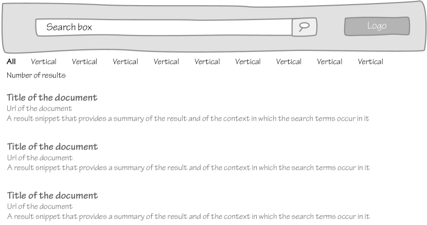
(a) A traditional ten blue links layout.

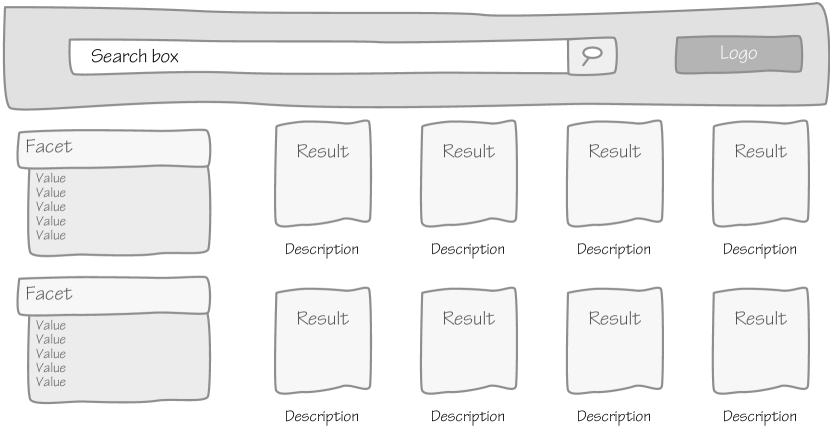
(b) A product search layout.

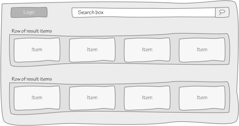
(c) A video recommendation layout.

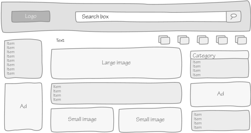
(d) An advertisement layout.

Figure 1. Examples of different ranking settings and result presentations.

The examples of result presentation layouts given in Fig. 1 are by no means an exhaustive list; moreover, new layouts and search settings continue to be introduced. The examples show that in some cases the top-down bias assumption of traditional LTR is misguided. Consequently, if there is a mismatch between the assumed preferred display order and the users’ preferences, the expected user experience will be degraded. If the wrong display order is assumed then even a ranker that perfectly predicts the relevance order may not display the most relevant document on the ideal position. We call settings where the ideal display order is unclear a priori complex ranking settings, because they involve a double algorithmic problem: both traditional relevance ranking as well as finding the best way to position the ranking. Thus, in these settings the task is both to infer the user preferred relevance order – what documents does the user want to see? – as well as the user preferred display order – in what order will the user consider the display positions? User behavior studies can help address this problem; for instance, the eye tracking studies listed above can reveal how users examine a layout and thus infer the preferred display order. Such user studies are expensive to perform at scale and it may be hard to find participants that represent the target user base well. Moreover, since layouts change often the results of previous studies may rapidly become obsolete.

As an alternative we investigate whether ranking in complex ranking settings can be learned from user interactions. We propose to use Deep Reinforcement Learning (RL), to infer a display order that best satisfies users, e.g., to infer that the most relevant document is to be displayed in the top-center in the case of a result layout as in Fig. 1(c). We introduce two approaches: (1) a standard GRU [6] that implicitly learns the preferred display order, and (2) a novel method that explicitly models a preference in display positions . We call the latter method the Double-Rank Model (DRM) since it learns how to rank the display positions and with which documents to fill those positions. Our experiments on three large publicly available LTR datasets show that only DRM is capable of successfully addressing complex ranking settings while all other methods are unable to break from the top-down assumption. As a result, DRM achieves the highest retrieval performance in all of the cases where the traditional top-down assumption does not hold while matching the state-of-the-art when the assumption does hold.

In this paper the following research questions are addressed:

1. Can existing ranking methods handle complex ranking settings?

2. Does DRM outperform existing methods in complex ranking settings?

2. Problem Setting

The idea of a complex ranking setting was introduced in Section 1; this section will formalize the concept and explain why traditional LTR methods are unable to deal with them.

2.1. Ranking settings

The core task in LTR is to order a set of documents to maximize the ease by which a user can perform their search task. Here we assume the user has a preferred order in which they consider the available documents $D=\{d_{1},\ldots d_{n}\}$. This order depends only on the documents and the user’s search task and thus we call this the preferred relevance order. Furthermore, documents are displayed to the user in a layout that has several positions for displaying them. We will assume that a layout has $k$ display positions $P=\langle p_{1},\ldots,p_{k}\rangle$, at each of which a single document can be presented. The user considers the display positions one by one, and is expected to do this in a certain order, i.e., subject to a certain position bias [13]. We interpret this order in display positions as the user’s preferred display order. Thus, in order to provide the optimal user experience, the most relevant document should be displayed in the position considered first, and so forth. In other words, documents must be displayed to the user so that there is a correspondence between the preferred relevance order and the display order. We call such a combination of a preferred relevance order and a preferred display order a ranking setting, and formally define it as follows:

Definition 2.1.

A ranking setting consists of a set of documents $D=\{d_{1},\ldots,d_{n}\}$, an ordered set of positions $P=\langle p_{1},\ldots,p_{k}\rangle$ as well as user preferences for positions ($>_{\mathit{pos}}$) and for documents ($>_{\mathit{doc}}$). The user has a preferred relevance order, so that all documents can be ordered according to their preference:

(1) $$d_{i}>_{\mathit{doc}}d_{j}>_{\mathit{doc}}\cdots>_{\mathit{doc}}d_{l}.$$

Similarly, positions can be ordered to their preferred display order:

(2) $$p_{i}>_{\mathit{pos}}p_{j}>_{\mathit{pos}}\cdots>_{\mathit{pos}}p_{l}.$$

Lastly, a ranking setting has an ideal ranking $R=[d_{i},\ldots,d_{j}]$, this is an ordering of the $k$ most preferred documents aligned with preference between display positions:

(3) $$\forall 0<i,j\leq k,\quad R_{i}>_{\mathit{doc}}R_{j}\leftrightarrow p_{i}>_{\mathit{pos}}p_{j}.$$

Thus, $R$ places the $i$-th most preferred document on the $i$-th most preferred position, for the top $k$ documents. Note that the ideal ranking $R$ is not necessarily the same as the preferred relevance order. While the most relevant document is always on the first position in the relevance order, its position in $R$ depends on the preferred display order.

2.2. Simple ranking settings

We define simple and complex ranking settings based on whether the display order is known a priori. In cases where it is known, the mismatch between the relevance order and the display order can always be avoided:

Definition 2.2.

A simple ranking setting is a ranking setting where the user’s preferred display order is known a priori. As a result, the ordered set of display positions $P=\langle p_{1},\ldots,p_{k}\rangle$ can be ordered to the users preferences so that:

(4) $$\forall 0<i,j\leq k,\quad i<j\leftrightarrow p_{i}>_{\mathit{pos}}p_{j}.$$

Consequently, the ideal ranking $R$ is then always aligned with the user preferred relevance order. Thus, if the document set $D$ is extended with one document: $D^{\prime}=D\cup\{d^{\prime}\}$, then in a simple ranking setting the ideal ranking for $D^{\prime}$, $R^{D^{\prime}}$, does not change the relative ordering of documents in $R^{D}$. Therefore, in a simple ranking setting the ideal ranking of $D^{\prime}$ is always the ideal ranking of $D$ with $d^{\prime}$ inserted at some position:

(5) $$R^{D^{\prime}}=[R^{D}_{1},R^{D}_{2},\ldots,R^{D}_{i},d^{\prime},R^{D}_{i+1},R^{D}_{i+2},\ldots].$$

The ten blue links layout is an example of a simple ranking setting, where the top-down display order is well studied [11]. Correspondingly, LTR has been very effective in this setting and has focused on finding the user’s preferred relevance order. Most LTR methods are based on functions that score documents independently and then rank documents according to their scores. This works well in simple ranking settings. For instance, consider four documents with the preferences:

(6) $$d_{1}>_{\mathit{doc}}d_{2}>_{\mathit{doc}}d_{3}>_{\mathit{doc}}d_{4},$$

and three display positions with the preferences:

(7) $$p_{1}>_{\mathit{pos}}p_{2}>_{\mathit{pos}}p_{3}.$$

The two sets $D=\{d_{1},d_{3},d_{4}\}$ and $D^{\prime}=\{d_{1},d_{2},d_{3},d_{4}\}$ have the following ideal rankings:

(8) $$R^{D}=[d_{1},d_{3},d_{4}],$$

(9) $$R^{D^{\prime}}=[d_{1},d_{2},d_{3}].$$

Thus any scoring function $f$ that correlates with the relevance order in the sense that $f(d_{1})>f(d_{2})>f(d_{3})>f(d_{4})$, will provide the ideal rankings for both cases. While this is usually not acknowledged explicitly, LTR methods have assumed that the ideal ranking should be aligned with the user’s preferred relevance order.

2.3. Complex ranking settings

Section 1 discussed several prevalent settings where the preferred display order is unclear. In these cases some performance is lost by the mismatch between the relevance order and the display order, as even when the most relevant documents are found they may not be displayed in the most efficient manner. We define the complex ranking setting by whether the display order is known a priori:

Definition 2.3.

A ranking setting where the user preferred display order is unknown a priori is called a complex ranking setting. Therefore, for the document sets $D$ and $D^{\prime}=D\cup\{d^{\prime}\}$, the ideal ranking of $D^{\prime}$, $R^{D^{\prime}}$, may change the relative ordering of documents in $D$ with respect to the ideal ranking of $D$, $R^{D}$, if the ranking setting is complex.

If we consider the same example as in Section 2.2 but change the display order from (7) to

(10) $$p_{2}>_{\mathit{pos}}p_{1}>_{\mathit{pos}}p_{3},$$

then the ideal rankings for $D=\{d_{1},d_{3},d_{4}\}$ and $D^{\prime}=D\cup\{d_{2}\}$ are:

(11) $$R^{D}=[d_{3},d_{1},d_{4}],$$

(12) $$R^{D^{\prime}}=[d_{2},d_{1},d_{3}].$$

Unlike the simple ranking setting discussed in Section 2.2, there is no function that can score documents independently and provide both ideal rankings: since such a function should provide $f(d_{3})>f(d_{1})$ in the case of $D$ and $f(d_{3})<f(d_{1})$ in the case of $D^{\prime}$. A possible solution would be a binary document scoring function that considers entire document set as one of its arguments, $f(d,D)$, thus allowing it to distinguish between $D$ and $D^{\prime}$. However, the computational costs of such a model that drops the document independence assumption would make it impossible to scale to any practical usage [18].

Instead, in Section 5 we propose another approach, one where the model sequentially selects a document and a position at which to place it. Thus, in contrast with LTR in the simple ranking setting, this method simultaneously learns both the relevance order and the display order.

3. Background

This section describes the RL concepts related to the novel methods that are introduced in Section 4 and 5.

3.1. Markov decision processes

RL methods are used to solve decision problem that can be modelled as Markov Decision Processess [26]. An MDP models a sequential decision process where an agent executes a chosen action at each time-step; the action will then affect the state of the world in the subsequent time-step. An MDP model consists of states $S$, actions $A$, transitions $T$, rewards $R$, and policies $\pi$. The states $S$ represents the set all possible states the process may be in at any time-step. The actions $A$ are the set of actions an agent can take at every time-step; this choice is the only part of the MDP the agent has direct control over. The transitions: after each time-step the state changes according to the action taken. These transitions are represented by the distribution $T(s_{t+1}\mid s_{t},a_{t})$. The rewards: the reward function $R$ provides the utility of taking an action in a state: $R(s,a)$. The policy: the actions of the agent are drawn from the policy distribution: $\pi(a\mid s)$.

The goal of an RL method is to find the policy that maximizes the expected (discounted) reward in future time steps:

(13) $$\begin{split}\mathbbm{E}[R(s_{t},a_{t})&+\gamma R(s_{t+1},a_{t+1})\\ &+\gamma^{2}R(s_{t+2},a_{t+2})+\ldots\mid S,A,T,R,\pi],\end{split}$$

where $0\leq\gamma\leq 1$ acts as a discount factor. Thus, the optimal policy should account for both the immediate reward it receives from an action but also the rewards it expects to receive from subsequent steps. This means that planning is involved in the decision process, which fits well with complex ranking settings where a relevant document should not always be placed on the first position.

3.2. Model-free reinforcement learning

The methods we introduce in Section 4 and 5 are based on the Deep Q-Network (DQN) [23]. DQN is a model free RL method; such methods do not explicitly model the transitions or rewards of the MDP. Instead they work with Q-values, which represent the expected value of a state-action pair: $Q(s,a)$ [26]. The value of a state-action pair is the immediate reward and the expected discounted future reward:

(14) $$Q(s,a) =R(s,a)+\gamma\sum_{s^{\prime}}T(s^{\prime}\mid s,a)\max_{a^{\prime}}Q(s^{\prime},a^{\prime}).$$

Thus, the Q-value of a state-action pair depends on the expected value of the next state. Here, the maximum over the actions is taken since the agent can be optimistic about its own action selection. To allow for generalization, in deep Q-learning these values are estimated by a model. Thus the weights $\theta$ should be found so that:

(15) $$Q(s,a,\theta) =R(s,a)+\gamma\sum_{s^{\prime}}T(s^{\prime}\mid s,a)\max_{a^{\prime}}Q(s^{\prime},a^{\prime},\theta).$$

Furthermore, DQN learns these values from experience, i.e., by executing its policy and recording its experience. At each time-step this gives a transition pair of the state $s$, action $a$, observed next state $s^{\prime}$, and observed reward $r$: $\langle s,a,r,s^{\prime}\rangle$. Then $\theta$ can be updated towards:

(16) $$Q(s,a,\theta) =r+\gamma\max_{a^{\prime}}Q(s^{\prime},a^{\prime},\theta).$$

Over time the Q-values will converge on the true values with the transitions $T$ and reward function $R$ implicitly learned. DQN uses an experience replay buffer [17] that keeps a large number of past transitions and updates on a batch sampled from this buffer. This mitigates the sequential dependency between recent experiences.

Another issue is that the model is updated towards a target that is predicted from its own weights, making the process very unstable. As a solution, DQN uses an older version of the model to predict future the Q-values from:

(17) $$Q(s,a,\theta_{T}) =r+\gamma\max_{a^{\prime}}Q(s^{\prime},a^{\prime},\theta_{L}),$$

where $\theta_{T}$ is being trained and $\theta_{L}$ is a previous set of weights. Periodically the $\theta_{T}$ is transferred to $\theta_{L}$: $\theta_{L}\leftarrow\theta_{T}$. As a result, the weights are updated to a target that remains stationary for long periods of time, stabilizing the learning process. Lastly, DQN is prone to over estimate certain Q-values, because the max operation is biased towards actions that are erroneously overestimated. As a solution, Van Hasselt et al. [28] proposed Double DQN, where the maximizing action is estimated on $\theta_{T}$:

(18) $$a^{\prime} =\operatornamewithlimits{arg\,max}_{a}Q(s^{\prime},a,\theta_{T})$$

(19) $$Q(s,a,\theta_{T}) =r+\gamma Q(s^{\prime},a^{\prime},\theta_{L}).$$

Thus, an overestimated value in $Q(s,a,\theta_{L})$ is less likely to be selected, since $\theta_{T}$ and $\theta_{L}$ are somewhat independent.

Algorithm 1 Double DQN [23, 28] a Model-Free RL method.

1:  Input: weights: $\theta_{0}$, replay size: $M$, transfer steps: $N$

2:  $E\leftarrow[]$ // initialize experience replay

3:  $\theta_{L}\leftarrow\theta_{0}$ // initialize label network

4:  for $i\in[1,2,\ldots,]$ do

5:     while $|E|<M$ do

6:        $\langle s,a,r,s^{\prime}\rangle\leftarrow\textit{execute\_policy}(\theta_{i})$

7:        $E\leftarrow append(E,\langle s,a,s^{\prime},r\rangle)$

8:     $\mathcal{L}\leftarrow 0$ // initialize loss function

9:     for $j\in[1,\ldots,\textit{batch\_size}]$ do

10:        $\langle s,a,r,s^{\prime}\rangle\leftarrow\textit{sample}(E)$ // sample without replacement

11:        $a^{\prime}\leftarrow\operatornamewithlimits{arg\,max}_{a}Q(s^{\prime},a,\theta_{i})$

12:        $\mathcal{L}\leftarrow\mathcal{L}+(Q(s,a,\theta_{i})-r-\gamma Q(s^{\prime},a^{\prime},\theta_{L}))^{2}$

13:     $\theta_{i+1}=\textit{gradient\_descent\_update}(\mathcal{L})$

14:     if $i\mod N=0$ then

15:        $\theta_{L}=\theta_{i}$

The full Double DQN procedure is displayed in Algorithm 1. At first, the Experience Replay buffer is empty (Line 2). Then the initial policy is executed until the buffer is filled to contain $M$ past transitions (Line 6). Subsequently, the loss $\mathcal{L}$ is initialized (Line 8) and several transitions are sampled from the replay buffer (Line 10). The maximizing action according to the train-network $\theta_{i}$ is determined (Line 11), and the loss is updated with the regression loss for the current Q-value according to the train-network and the estimated value according to the label-network:

(20) $$(Q(s,a,\theta_{i})-r-\gamma Q(s^{\prime},a^{\prime},\theta_{L}))^{2}.$$

The weights are updated according to the calculated loss (Line 13) providing a new model $\theta_{i+1}$. After $N$ update steps the label network is replaced with a copy of the current training network (Line 15). When the Q-values have been learned, the estimated optimal policy is derived by taking the maximizing action for each state.

4. Reinforcement Learning to Rank

This section introduces a baseline approach to the complex ranking setting. First Section 4.1 discusses how LTR can be approached as an RL problem, then Section 4.2 introduces a baseline approach to the problem.

Algorithm 2 Sampling an episode with the baseline GRU model.

1:  $\mathbf{D}_{q}\leftarrow\textit{receive\_query}$ // query and pre-selection of doc.

2:  $\mathbf{h}_{0}\leftarrow\mathbf{0}$ // initialize hidden state

3:  $\mathbf{R}\leftarrow[]$

4:  for $t\leftarrow 1\ldots k$  do

5:     if coinflip with $\epsilon$ probability then

6:        $\mathbf{d}_{t}\leftarrow\textit{sample\_document}(\mathbf{D}_{q})$ // explorative action

7:     else

8:        $\mathbf{q}\leftarrow[0,\ldots,0]$ // initialize zero document score vector

9:        for $d_{i}\in\mathbf{D}_{q}$  do

10:           $\mathbf{h}^{\prime}\leftarrow GRU(\mathbf{h}_{t-1},\mathbf{d}_{i})$

11:           $\mathbf{q}_{i}\leftarrow Q(h^{\prime},d_{i},\theta)$ // estimate Q-value for doc. (Eq 30)

12:        $i\leftarrow\operatornamewithlimits{arg\,max}{\mathbf{q}}$ // select doc. with highest q-value

13:        $\mathbf{R}_{t}\leftarrow\textit{gather}(\mathbf{D}_{q},d_{i})$ // add doc. to SERP

14:     $\mathbf{D}_{q}\leftarrow\textit{remove}(\mathbf{D}_{q},\mathbf{d}_{t})$ // remove to prevent duplicates

15:     $\mathbf{h}_{t}=GRU(\mathbf{h}_{t-1},\mathbf{d}_{t})$ // update (partial) SERP embedding

16:  return  $\mathbf{R}$

4.1. Ranking as a Markov decision process

LTR has been approached as an RL problem in the past [30, 31]; notably Xia et al. [31] used a policy gradient method for search result diversification. The methods introduced in this paper are based on Q-learning instead of policy gradients, however they also approach ranking as an MDP.

The complex ranking setting is defined by the user preferred display order being unknown a priori. As a result, it is impossible to acquire labelled data, e.g., from human annotators. As an alternative, we will use RL to learn from user interactions. First, the ranking problem must be formalized as an MDP; as described in Section 3.1, this means that states $S$, actions $A$, transitions $T$ and rewards $R$ have to be specified. In this paper, we approach ranking as a sequential decision problem, where every document in a ranking is seen as a separate decision. Accordingly, the states $S$ encode the query information and all possible partial rankings; the initial state $s_{0}$ represents the query and an empty ranking. The actions $A$ consist of the available documents $D_{q}$, with the exception of documents already in $s_{t}$ to prevent duplicate placement. The transitions $T$ are deterministic between the partial rankings in $S$: adding a document $d^{\prime}$ to $s_{t}=(q,[d_{1},\ldots,d_{i}])$ transitions to $s_{t+1}=(q,[d_{1},\ldots,d_{i},d^{\prime}])$ exclusively. Since no ranking in $S$ exceeds the number of display positions $k$, every episode lasts $k$ steps and any state $s_{t}$ at time step $t=k$ is an end-state. Lastly, the rewards $R$ can be given at the document-level or at the SERP-level; for a chosen discount function, the document level reward is given by:

(21) $$R_{\mathit{doc}}(s_{t},a_{t})=\frac{2^{\mathit{rel}(d_{a_{t}})-1}}{\mathit{discount}(t)}.$$

The discount function can be chosen to match the Discounted Cumulative Gain (DCG): $\mathit{discount}(i)=\log_{2}(i+1)$. However, other discount functions can simulate different complex ranking settings. The SERP-level reward is only given for actions that complete rankings and simply sums the document-rewards in the ranking:

(22) $$R_{\mathit{SERP}}(s_{t},a_{t})=\begin{cases}0,&t<k\\ \sum^{k}_{i=1}R_{\mathit{doc}}(s_{i},a_{i}),&t=k.\\ \end{cases}$$

The SERP-level reward simulates challenging settings where the reward cannot be broken down to the document level. Since every episode is limited to $k$ steps, future rewards are not discounted, that is, $\gamma=1$. So the aim of the policy is to maximize the expected reward over the entire episode.

4.2. A baseline approach to complex ranking

In order to use Deep Q-Learning on the complex ranking setting, a model that can estimate Q-values is required. This section will introduce a baseline estimator, before Section 5 introduces a novel model specialized for the complex ranking setting.

Since ranking is approached as a sequential process, a Recurrent Neural Network (RNN) is used to encode the ranking so far and estimate the value of adding the next document. Unlike previous work [30, 31], we use a GRU [6] instead of a plain RNN. The benefit of a GRU is that, similar to a Long Short-Term Memory Network (LSTM) [10], it has a form of explicit memory, allowing it to remember values over multiple iterations in the sequence. Compared to the LSTM model a GRU has fewer parameters since it only has an update gate vector $z_{t}$ and reset gate vector $r_{t}$. The GRU model can be formulated as follows:

(23) $$\mbox{}z_{t} =\sigma(W_{z}x_{t}+U_{z}h_{t-1}+b_{z}),$$

(24) $$\mbox{}r_{t} =\sigma(W_{r}x_{t}+U_{r}h_{t-1}+b_{r}),$$

(25) $$\mbox{}h_{t} =GRU(h_{t-1},x_{t})$$

(26) $$=z_{t}\circ h_{t-1}+(1-z_{t})\circ\tanh(W_{h}h_{t-1}+U_{h}(r_{t}\circ h_{t-1})+b_{h})\mbox{}$$

where $\circ$ is the Hadamard product and the matrices $W$, $U$ and vectors $b$ are the weights to be optimized.

It would make sense to start the Q-value estimation by encoding the query $\mathbf{q}$. Unfortunately, no query-level features are available in public LTR datasets (Section 6.1), thus we use zero initialization for the hidden state:

(27) $$h_{0} =\mathbf{0}.$$

Then, for all the documents pre-selected for the query $D_{q}$ an embedding is made, with $\sigma$ as the Rectified Linear Unit (ReLU) function and document feature vector $\mathbf{d}$:

(28) $$\mathbf{\widehat{d}}=\sigma(W_{d}\mathbf{d}+b_{d}).$$

These document representations are shared for each step in the process; if at time-step $t$ the document $d$ is selected the Q-value is calculated as follows:

(29) $$h_{t} =GRU(h_{t-1},\mathbf{\widehat{d}}),$$

(30) $$Q(s_{t},d_{t},\theta) =v_{q}^{T}\sigma(W_{q}h_{t}+b_{q})+u_{q},$$

where the matrix $W_{q}$, the vectors $v_{q}$, $b_{q}$ and scalar $u_{q}$ are weights to be optimized.

For clarity, Algorithm 2 describes the policy in detail; an epsilon greedy approach is used to account for exploration, meaning that at every time step a random action is performed with probability $\epsilon$. Initially the ranking $\mathbf{R}$ is empty (Line 3). For $k$ iterations with probability $\epsilon$ a document is uniformly sampled (Line 6). Otherwise, the Q-value for adding a document is computed for every available document (Line 11). The document with the highest Q-value is added to the SERP (Line 15) and removed from the set of available documents (Line 14); this prevents it from appearing twice in $\mathbf{R}$. Finally, after $\mathbf{R}$ is completed, it is used by DQN (Algorithm 1); DQN interprets every document placement as an action as described in Section 4.1.

Since this approach sequentially decides whether to place documents, it could learn a policy that does not place the most relevant document first. Potentially, it could wait until the best display position before placing it. The risk here is that if it saves more relevant documents than positions left to fill, some of them will not be displayed.

Algorithm 3 Sampling an episode with DRM.

1:  $\mathbf{D}_{q}\leftarrow\textit{receive\_query}$ // query and pre-selection of doc.

2:  $\mathbf{P}\leftarrow[p_{1},\ldots,p_{k}]$ // available positions

3:  $h_{0}\leftarrow\mathbf{0}$ // initialize hidden state

4:  $\mathbf{R},\mathbf{I}\leftarrow[],[]$ // initialize ranking and selected positions

5:  for $t\leftarrow 1\ldots k$  do

6:     if coinflip with $\epsilon$ probability then

7:        $\mathbf{d}_{t}\leftarrow\textit{sample\_document}(\mathbf{D}_{q})$ // explorative doc. action

8:     else

9:        // find the document with highest Q-value (Eq. 36)

10:        $\mathbf{R}_{t}\leftarrow\operatornamewithlimits{arg\,max}_{d_{i}\in\mathbf{D}_{q}}{Q(h_{t-1},d_{i},\theta)}$

11:     $\mathbf{D}_{q}\leftarrow\textit{remove}(\mathbf{D}_{q},\mathbf{R}_{t})$ // remove to prevent duplicates

12:     if coinflip with $\epsilon$ probability then

13:        $\mathbf{p}_{t}\leftarrow\textit{sample\_position}(\mathbf{P})$ // explorative pos. action

14:     else

15:        // find the position with highest Q-value (Eq. 37)

16:        $\mathbf{P}_{t}\leftarrow\operatornamewithlimits{arg\,max}_{p_{i}\in\mathbf{P}}{Q(h_{t-1},\mathbf{R}_{t},p_{i},\theta)}$

17:     $\mathbf{P}\leftarrow\textit{remove}(\mathbf{P},\mathbf{p}_{t})$ // make position unavailable

18:     $\mathbf{h}_{t}=GRU(\mathbf{h}_{t-1},\mathbf{d}_{t},\mathbf{p}_{t})$ // update (partial) SERP embedding

19:  return  $\mathbf{R},\mathbf{I}$

5. Double-Rank for Complex Ranking

Section 4.2 used a standard GRU to sequentially choose what documents to place. In this section we introduce a method that sequentially chooses a document and then a display position to place it in. This approach explicitly models the duality of the complex ranking setting: the preferred relevance order and the preference in display positions. Because it ranks both documents and positions we call it the Double-Rank Model (DRM). The key insight behind DRM is that by choosing in what order to fill display positions, it can avoid having to save a good document for a later position. Since it can start placement at the most preferred position. DRM produces a list of documents $\mathbf{R}$ and a list of positions $\mathbf{I}$; the SERP is then created by placing the documents in $\mathbf{R}$ according to $\mathbf{I}$. Thus, the selection of $\mathbf{R}$ encapsulates the inferred relevance order and the choice of $\mathbf{I}$ captures the inferred display order.

5.1. Changing the MDP for DRM

The MDP as described in Section 4.1 has to be altered to accommodate the DRM approach. Firstly, the states $S$ now include every (partial) ranking of documents $\mathbf{R}$ and every (partial) matching set of positions $\mathbf{I}$. We arbitrarily choose documents to be selected before their positions, thus at the first state a document is added to $\mathbf{R}$ and at the next state its position is added to $\mathbf{I}$. The actions $A$ also consist of either choosing a document or index depending on the state $s_{t}$. In other words, if at time step $t$ a document is chosen ($a_{t}\in D_{q}$), then at the next step its position is chosen ($a_{t+1}\in P$). Similarly, the transitions $T$ are deterministic between the states: adding a document $d^{\prime}$ transitions the state from $s_{t}=(q,[d_{1},\ldots,d_{i}],[p_{1},\ldots,p_{i}])$ to $s_{t+1}=(q,[d_{1},\ldots,d_{i},d^{\prime}],[p_{1},\ldots,p_{i}])$ exclusively. Likewise, choosing a position $p^{\prime}$ transitions it from $s_{t}=(q,[d_{1},\ldots$, $d_{i}]$, $[p_{1},\ldots$, $p_{i-1}])$ to $s_{t+1}=(q$, $[d_{1},\ldots,d_{i}],[p_{1},\ldots,p_{i-1},p^{\prime}])$. As a result, every episode now consists of $2k$ steps. Finally, the reward function has to be adapted slightly. For the document-level reward this becomes:

(31) $$R_{doc}(s_{t},a_{t})=\begin{cases}0,&a_{t}\in D_{q}\\ \frac{2^{\textit{rel}(d_{a_{t-1}})-1}}{\textit{discount}(p_{a_{t}})}&a_{t}\in P,\\ \end{cases}$$

where $p_{a_{t}}$ is the selected position at $t$ and $d_{a_{t-1}}$ is the corresponding document selected at the previous step. The discount here only depends on the selected position and not on what time-step it was placed there. The SERP-level reward becomes:

(32) $$R_{\mathit{SERP}}(s_{t},a_{t})=\begin{cases}0,&t<2k\\ \sum^{2k}_{i=1}R_{doc}(s_{i},a_{i}),&t=2k.\end{cases}$$

While the reward function is different for the DRM, every SERP receives the same total reward as in the baseline MDP (Section 4.1).

5.2. The Double-Rank model

With the DRM-MDP defined, we can now formulate the model that estimates Q-values and thus learns the ranking policy. Similar to the baseline model (Section 4.2), the DRM uses a GRU network to encode the state. First the hidden state is initialized:

(33) $$h_{0} =\mathbf{0}.$$

Then an embedding for every document is made, given the document feature vector $\mathbf{d}$:

(34) $$\mathbf{\widehat{d}}=\sigma(W_{d}\mathbf{d}+b_{d}).$$

Instead of alternating the input of the GRU with representations of documents or positions, we only update the hidden state $h_{t}$ after every position action. As an input the embedding of the previously chosen document $\mathbf{\widehat{d}}_{t-1}$ and position $p_{t}$ are concatenated:

(35) $$h_{t} =GRU(h_{t-2},[\mathbf{\widehat{d}}_{t-1},p_{t}]),$$

where each position $p_{t}$ is represented by a unique integer.

The Q-values for document actions and position actions are computed differently; both use the concatenation of the last hidden state and the corresponding document embedding: $[h_{t-1},\mathbf{\widehat{d}}_{t}]$. For a document action the Q-value is calculated by:

(36) $$Q(s_{t},d_{t},\theta) =v_{q}^{T}\sigma(W_{q}[h_{t-1},\mathbf{\widehat{d}}_{t}]+b_{q})+u_{q},$$

The computation for position action $p_{t}$ in the subsequent time-step uses the same concatenation (now denoted as $[h_{t-2},\mathbf{\widehat{d}}_{t-1}]$):

(37) $$Q(s_{t},p_{t},\theta) =v_{p_{t}}^{T}\sigma(W_{p}[h_{t-2},\mathbf{\widehat{d}}_{t-1}]+b_{p})+u_{p_{t}},$$

where the vectors $v_{p_{t}}$ and scalar $u_{p_{t}}$ are unique for the position $p_{t}$. Since the number of positions is limited, we found it more effective to use unique weights for each of them, in terms of both computational efficiency and learning speed.

The DRM policy is displayed in Algorithm 3; the document ranking $\mathbf{R}$ and position ranking $\mathbf{I}$ are initialized (Line 4). Then for $k$ iterations a document and position are selected subsequently. First, with an $\epsilon$ probability a random document is selected as an exploratory action (Line 7). Otherwise, the document with the highest estimated Q-value is selected (Line 10). It is then removed from the available set $D_{q}$ to prevent duplicate placement. Subsequently, with an $\epsilon$ probability an exploratory position is selected (Line 13). Otherwise, the position with the highest Q-value is selected (Line 16); note that this value depends on the previously selected document. The position is then made unavailable for subsequently selected documents (Line 17). When $k$ documents and positions have been selected, the rankings $\mathbf{R}$ and $\mathbf{I}$ are passed to the DQN (Algorithm 1). The user will be shown the documents in $\mathbf{R}$ in the display positions according to $\mathbf{I}$. Given a weak reward signal the choice of both $\mathbf{R}$ and $\mathbf{I}$ can be optimized using DQN.

6. Experimental Setup

This section describes the experiments that were run to answer the research questions posed in Section 1.

6.1. Datasets

Our experiments are performed over three large publicly available LTR datasets [24, 5, 8]; these are retired validations sets published by large commercial search engines. Each dataset consists of queries, documents and relevance labels. For every query there is a preselection of documents; while queries are only represented by their identifiers, feature representations and relevance labels are available for every preselected document-query pair. Relevance labels range from not relevant (0) to perfectly relevant (5), and each dataset is divided into training, validation and test partitions.

Firstly, we use the MSLR-WEB30k dataset released by Microsoft in 2010 [24]. It consists of 30,000 queries obtained from a retired labelling set of the Bing search engine. The dataset uses 136 features to represent its documents; each query has 125 assessed documents on average. This dataset is distributed in five folds for cross-fold validation. Secondly, also in 2010, Yahoo! organized a public Learning to Rank Challenge [5] with an accompanying dataset. This set consists of 709,877 documents encoded in 700 features and sampled from query logs of the Yahoo! search engine, spanning 29,921 queries. Thirdly, in 2016 the Istella search engine released a LTR dataset to the public [8]. It is the largest dataset to date with a total of 33,118 queries, an average of 315 documents per query and 220 features. Only a training and test partition were made available for this dataset; for parameter tuning we sampled 9,700 queries from the training partition and used them as a validation set.

6.2. Simulating complex ranking settings

Our experiments are based around a stream of queries, for every received query the system presents the user a SERP generated by the policy (Algorithm 2 or 3). The SERP is displayed to the user in a $k=10$ position display. The system then receives a reward signal from the user, indicative of their satisfaction. These interactions are passed to the DQN (Algorithm 1) which stores them in the experience replay buffer. When the buffer is sufficiently full, a batch of interactions is sampled and the model is updated accordingly. The stream of queries is simulated by uniformly sampling queries from the datasets. The reward signal is simulated by the function described in Section 4.1 or 5.1, where the $\mathit{discount}$ function is varied to simulate different complex ranking settings. All of the $\mathit{discount}$ functions we use are based on Discounted Cumulative Gain (DCG); we assign every position $p_{i}$ an integer index and then define:

(38) $$\mathit{discount}(p_{i}) =\log_{2}(p_{i}+1).$$

Here, the integer $p_{i}$ is the index the position has in the user preferred display order. Thus, the first observed position will be discounted by $\textit{discount}(1)$, and so on. Then we use three display orders as displayed in Table 1. First, first-bias simulates a user who considers positions in the assumed order, resulting in a standard DCG reward signal. Then center-bias simulates a user who considers the center position first, e.g., as can happen in a horizontal display. Lastly, we consider the last-bias preference order, where the last position is considered first, this simulates the worst-case scenario as the display order is the furthest removed from the assumed order.

Note that no method is initially aware of what the display order is; the only indirect indication of the preferred order comes from the received rewards.

Table 1. Three different display order preferences used to simulate different complex ranking settings. The $p_{i}$ indicate positions and the numerical values in the cells and the intensity of the color indicate preferred display order. E.g., in the first-bias preference, $p_{1}$ is the most preferred position and $p_{10}$ the least preferred position.

	$p_{1}$	$p_{2}$	$p_{3}$	$p_{4}$	$p_{5}$	$p_{6}$	$p_{7}$	$p_{8}$	$p_{9}$	$p_{10}$
first-bias	010	020	030	040	050	060	070	080	090	10
center-bias	090	070	050	030	010	020	040	060	080	10
last-bias	10	090	080	070	060	050	040	030	020	010

For evaluation we use the mean normalized reward, which we call the Permuted Normalized DCG (P-NDCG). This is the received reward divided by the maximum possible reward:

(39) $$\textit{P-NDCG}=\frac{\sum_{t=1}^{k}R(s_{t},a_{t})}{\max_{[a^{\prime}_{0},\ldots,a^{\prime}_{k}]}\sum_{t=1}^{k}R(s_{t}^{\prime}a_{t}^{\prime})}.$$

This reward can be seen as NDCG where the discount indices have been permuted. Note that in the first-bias case, P-NDCG is the equivalent of regular NDCG. Lastly, to evaluate the estimated optimal behavior, P-NDCG is computed without exploration: $\epsilon=0$.

6.3. Experimental runs

Runs were created with DRM (Section 5), the baseline GRU (Section 4), and the MDP-DIV model [31]. The latter model was introduced for search result diversification; however, by changing the reward function it can be applied to the complex ranking setting. Runs were performed on the three datasets, each with one of the three reward signals described in Section 6.2, both at the document-level and at the SERP-level. Thus there are 27 dataset-model-reward combinations; five runs were performed for each combination from which the mean results are reported. Significance testing was done using a single-tailed T-test.

Parameter tuning was done on the validation sets; the learning rate was tuned between $10^{-2}$ and $10^{-5}$ per dataset; models were updated with early stopping up to 200,000 steps. The other parameters were the same for each dataset: the experience replay buffer size was 5,000; the number of steps between transfers was set to 5,000; the exploration degree $\epsilon$ was initialized at $1.0$ and degraded to $0.05$ over 30,000 iterations. The weights were chosen so that every document representation $\mathbf{\widehat{d}}$ of size $128$, the hidden states $h_{t}$ of size $256$, and the vectors $v_{q}$ and $v_{p}$ have size $128$. Gradient descent was performed using Adam optimization with batches of $64$ episodes. All transitions sampled from an episode are included in a batch for computational efficiency. Our implementation, including parameter settings, are publicly available to ensure reproducibility.

7. Results

In this section we answer the research questions posed in Section 1 by discussing the results from our experiments. As a reminder, these questions are: do existing methods perform well in complex ranking settings (RQ1); and does DRM outperform them in these settings (RQ2). Additionally, we also compare the performance of methods under a document-level and SERP-level reward.

Our main results are displayed in Table 2, which shows the average P-NDCG for each method and reward signal. Figure 2 also displays the average relevance label per position for a GRU baseline model and DRM on the Istella dataset under SERP-level rewards.

Table 2. Average normalized rewards for two baseline models and DRM under different complex ranking settings and reward signals. Bold values indicate the best performance per dataset and setting. Significant positive differences are indicated by ^▲($p<0.01$) and ^△($p<0.05$), significant negative differences by ^▼and ^▽, respectively. In the table, the first symbol indicates the significance of a difference between DRM and MDP-DIV, the second between DRM and GRU.

	MSLR			Yahoo			Istella
	first-bias	center-bias	last-bias	first-bias	center-bias	last-bias	first-bias	center-bias	last-bias
	Document-Level Reward
MDP-DIV	0.423 ($0.002$) ▼▼	0.360 ($0.004$) ▼▼	0.339 ($0.003$) ▼▼	0.716 ($0.004$) ▼▼	0.620 ($0.003$) ▼▼	0.587 ($0.004$) ▼▼	0.579 ($0.003$) ▼▼	0.451 ($0.002$) ▼▼	0.399 ($0.002$) ▼▼
GRU	0.433 ($0.012$) ▼▼	0.388 ($0.002$) ▼▼	0.369 ($0.003$) ▼▼	0.722 ($0.004$) ▼▼	0.656 ($0.001$) ▼▼	0.600 ($0.002$) ▼▼	0.623 ($0.002$) ▼▼	0.532 ($0.003$) ▼▼	0.444 ($0.002$) ▼▼
DRM	0.444 ($0.004$) ▲-	0.444 ($0.005$) ▲▲	0.445 ($0.004$) ▲▲	0.728 ($0.002$) ▲▲	0.721 ($0.001$) ▲▲	0.725 ($0.001$) ▲▲	0.627 ($0.001$) ▲△	0.624 ($0.003$) ▲▲	0.627 ($0.004$) ▲▲
	SERP-Level Reward
MDP-DIV	0.414 ($0.004$) ▼▼	0.360 ($0.006$) ▼▼	0.338 ($0.003$) ▼▼	0.702 ($0.002$) ▼▼	0.611 ($0.002$) ▼▼	0.584 ($0.000$) ▼▼	0.549 ($0.010$) ▼▼	0.438 ($0.005$) ▼▼	0.389 ($0.005$) ▼▼
GRU	0.402 ($0.004$) ▼▼	0.367 ($0.015$) ▼▼	0.344 ($0.003$) ▼▼	0.708 ($0.003$) ▼▼	0.625 ($0.004$) ▼▼	0.599 ($0.003$) ▼▼	0.522 ($0.007$) ▼▼	0 .449 ($0.008$) ▼▼	0.422 ($0.004$) ▼▼
DRM	0.395 ($0.003$) ▼▼	0.390 ($0.016$) ▲△	0.384 ($0.013$) ▲▲	0.669 ($0.016$) ▼▼	0.635 ($0.004$) ▲▲	0.647 ($0.012$) ▲▲	0.533 ($0.010$) ▲▽	0.532 ($0.011$) ▲▲	0.534 ($0.007$) ▲▲

7.1. Baseline performance

First, we answer RQ1 by looking at the performance of the MDP-DIV and GRU baseline methods. Table 2 shows that across all datasets there is a substantial difference in performance between the ranking settings. As expected, both MDP-DIV and GRU perform best in the first-bias settings, where their assumed display order matches the preferred order in the setting. Conversely, performance is significantly worse in the center-bias and last-bias settings. On the Yahoo and Istella datasets this difference can go up to $0.1$ P-NDCG, under both document-level and SERP-level rewards. This shows that the performance of both baselines is heavily affected by the preferred display order, and in situations where this order is unknown this can lead to a substantial drop in performance.

To better understand the drop in performance of the GRU baseline, we look at Figure 2(a). Here we see that the reward signals do affect the ranking behaviour the GRU learns. For instance, in the center-bias case the most preferred display positions ($p_{5}$) has the highest average relevance label. However, the complete preferred display order does not seem to be inferred correctly. Notably, the relevance on the first three positions ($p_{1},p_{2},p_{3}$) is compromised, i.e., position $p_{3}$ is preferred over $p_{8}$ but has a much lower average relevance label. It seems that GRU intentionally ranks worse at the start of the ranking so that the most relevant documents are not placed too early. This behavior places the most relevant document on the most preferred position, but sacrifices the relevance at earlier positions. Thus, the GRU baseline is unable to rank for the center-bias display order. Moreover, in the last-bias setting $p_{3}$ has the highest average relevance while $p_{10}$ is the most preferred display position. GRU appears to be unable to follow this preferred display order and, instead, optimizes for the relevance order only.

Due to the significant decreases in performance that are observed for the MDP-DIV and GRU baseline models in different ranking settings, we answer RQ1 negatively and conclude that neither baseline model performs well in complex ranking settings.

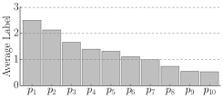
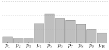
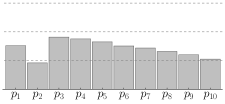
(a) Average label per position for the GRU baseline model in different settings: first-bias(left), center-bias (middle) and last-bias (right).

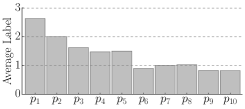
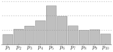
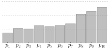
(b) Average label per position for the DRM in different settings: first-bias(left), center-bias (middle) and last-bias (right).

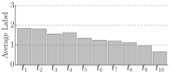
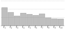
(c) Average label per time-step for the DRM in different settings: first-bias(left), center-bias (middle) and last-bias (right).

Figure 2. Average label per position for a single GRU baseline model and a single DRM trained on the Istella dataset in different complex ranking settings under SERP-level rewards.

7.2. DRM performance on complex rankings

In order to answer RQ2, we consider the performance of DRM reported in Table 2. In the first-bias setting the DRM performs similarly to the baseline models across all datasets. While under SERP-level rewards the performance varies per dataset, under document-level rewards DRM performs better than the baseline methods in all cases. The performance of DRM in the center-bias and last-bias settings is significantly better than the baseline models, with a substantial difference of over $0.1$ P-NDCG in multiple cases. Thus, if there is a SERP-level reward signal and the user preferred display order is non-standard then DRM significantly outperforms the baseline methods. Under decomposable rewards DRM achieves the best ranking performance regardless of the preferred display order.

Furthermore, Table 2 shows that the performance of DRM is not affected by the preferred display order. Unlike the baseline methods, DRM performs similarly in the first-bias, center-bias and last-bias settings. DRM differs from the baselines by not having an assumed display order, and therefore it also does not have a disadvantage in any of the settings. Thus, by being able to determine the order in which positions are filled, DRM can maintain its performance in any complex ranking setting. This is further illustrated in Figure 2(b): DRM correctly identifies the preferred display order for each complex ranking setting. In all three cases, the more preferred positions have a higher average relevance label, with only a few minor errors in the inferred order of less preferred positions. Then, Figure 2(c) displays the average relevance label of the document DRM selects per time-step; in all settings, the first placed documents are the most relevant. DRM follows the preferred relevance order when selecting documents, but places them in positions according to the preferred display order. Thus, as hypothesized, DRM does not save relevant documents for later time-steps; we attribute the better performance of DRM to this difference.

In conclusion, we answer RQ2 positively. DRM outperforms the baseline methods in settings where the preferred display order is unknown. By looking at the average relevance label per position, we see that DRM correctly infers the preferred order in all cases. Consequently, by correctly inferring both the relevance and display order DRM performs consistently well in all complex ranking settings.

7.3. Document-level vs. SERP-level rewards

Lastly, we briefly discuss the difference in performance between document-level rewards and SERP-level rewards. Table 2 shows that all methods perform better under document-level rewards. This is expected since under SERP-level rewards the methods have to infer how the reward signal is decomposed, while with document-level rewards this decomposition is directly observed. Under SERP-level rewards in the first-bias setting, it is also less clear what the best performing method is, as it varies per dataset. Conversely, under document-level rewards the DRM method reaches the highest performance across all datasets. However, despite all methods performing less well under SERP-level rewards, the DRM still has the best performance on the center-bias and last-bias settings. Figure 2(b) shows that the DRM is capable of inferring the correct display order from the less informative SERP-level reward signal. Thus, even with very weak reward signals DRM is robust to display preferences in complex ranking settings.

8. Related Work

We discuss research related to complex ranking settings: whole page optimization and ranking for alternative presentations formats.

8.1. Whole page optimization

In recent years, the ten blue links format has become less prominent and search engines now usually display a selection of images, snippets and information boxes along their search results [29]. As SERPs contain more alternative items, their evaluation has changed accordingly. Previous work has looked at whole page evaluation, where either human judges [2] or user models [7] are used to evaluate the entire SERP. Such user models consider the possibility that users may direct their attention to information boxes or snippets in the SERP. As a result, they can recognize that some forms of user abandonment can be positive, because the user can be satisfied before clicking any links.

Wang et al. [29] introduced the idea of whole page presentation optimization, where the entire result presentation is optimized, including item position, image size, text font and other style choices. While this method addresses the importance of user presentation preferences, it does not decide what items to display, but assumes this set is given. The method assumes that the number of possible presentation formats is small enough to iterate over. In the complex ranking setting this would lead to combinatorial problems as for a layout with $k$ positions there are $k!$ preferred display orders possible. While this work optimizes result presentation, it does not consider the mismatch between the user preferred relevance order and display order.

8.2. Alternative presentation formats

Section 1 has already discussed a number of different search settings and layouts. While this paper has focussed on optimizing for the relevance and display preferences of users, previous work has looked at optimizing ranking for specific alternative presentations. For instance, SERPs in mobile search generally use single column vertical layouts for the relatively small mobile screens. Luo et al. [20] recognize that the percentage of the screen an item covers should be taken into evaluation and propose an evaluation method that discounts items according to the varying lengths.

In addition, existing work on optimizing display advertisement placement has noted that presentation context can have a big impact on the click-through-rate of an ad. For instance, Metrikov et al. [21] found that whole-page-satisfaction leads to higher click-through-rates on the ad block of SERPs. Furthermore, ads can be more effective if they are optimized to display multiple products at once [16], or if multiple banners display the related advertisements [9].

Similar to the concept of complex ranking settings, these existing studies show that for the best user experience the presentation of a ranking should be optimized together with its content.

9. Conclusion

In this paper we have formalized the concept of a complex ranking setting, where the user has a preferred relevance order – an ordering of documents – and a preferred display order – a preference concerning the positions in which the documents are displayed. The ideal ranking in a complex ranking setting matches the relevance order with the display order, i.e., where the most relevant document is displayed in the most preferred position, and so forth. Thus these settings pose a dual problem: for the optimal user experience both the relevance order and the display order must be inferred. We simulate this setting by performing experiments where a permuted DCG is given as a reward signal, e.g., in the last-bias ranking setting the last display position is discounted as if it was the most preferred position according to the user.

Our experiments show that existing methods are unable to handle the complex ranking setting. Our results show that while existing methods learn different behaviors in different settings, they are unable to rank documents according to any non-standard preferred display order. As an alternative, we have introduced DRM, which sequentially selects documents and the positions to place them on. By explicitly modeling the duality between the relevance order and display order, DRM is able to infer the user preferred display order and relevance order simultaneously. Our results show that DRM matches state-of-the-art performance in settings where the display order is known, and significantly outperforms previous methods in complex ranking settings. Thus, when dealing with complex presentation layouts where it is unclear in what order users consider display positions, DRM is able to provide good performance regardless of the users’ actual display preferences.

Future work could consider more noisy reward signals; while our setup simulates complex ranking settings, it does so without noise in the reward signal. Even under these ideal circumstances existing methods are unable to infer non-standard preferred display orders. It would be interesting to investigate whether DRM is still able to handle complex ranking settings with high levels of noise. Lastly, the deployment of DRM on an actual search setting could show the impact display preferences have on user experiences.

Code

To facilitate reproducibility of the results in this paper, we are sharing the code used to run the experiments in this paper at https://github.com/HarrieO/RankingComplexLayouts.

Acknowledgements

This research was supported by Ahold Delhaize, Amsterdam Data Science, the Bloomberg Research Grant program, the China Scholarship Council, the Criteo Faculty Research Award program, Elsevier, the European Community’s Seventh Framework Programme (FP7/2007-2013) under grant agreement nr 312827 (VOX-Pol), the Google Faculty Research Awards program, the Microsoft Research Ph.D. program, the Netherlands Institute for Sound and Vision, the Netherlands Organisation for Scientific Research (NWO) under project nrs CI-14-25, 652.002.001, 612.001.551, 652.001.003, and Yandex. All content represents the opinion of the authors, which is not necessarily shared or endorsed by their respective employers and/or sponsors.

References

- [1]
- Bailey et al. [2010] Peter Bailey, Nick Craswell, Ryen W. White, Liwei Chen, Ashwin Satyanarayana, and S.M.M. Tahaghoghi. 2010. Evaluating whole-page relevance. In SIGIR. ACM, 767–768.
- Buscher et al. [2010] Georg Buscher, Susan Dumais, and Edward Cutrell. 2010. The good, the bad, and the random: an eye-tracking study of ad quality in web search. In SIGIR. ACM, 42–49.
- Campion [2013] Matthew Campion. 2013. Amazon.com product search and navigation eye tracking study. https://www.looktracker.com/blog/eye-tracking-case-study/amazon-com-product-search-and-navigation-eye-tracking-study/.
- Chapelle and Chang [2011] Olivier Chapelle and Yi Chang. 2011. Yahoo! Learning to Rank Challenge Overview. Journal of Machine Learning Research 14 (2011), 1–24.
- Cho et al. [2014] Kyunghyun Cho, Bart Van Merriënboer, Caglar Gulcehre, Dzmitry Bahdanau, Fethi Bougares, Holger Schwenk, and Yoshua Bengio. 2014. Learning phrase representations using RNN encoder-decoder for statistical machine translation. arXiv preprint arXiv:1406.1078 (2014).
- Chuklin and de Rijke [2016] Aleksandr Chuklin and Maarten de Rijke. 2016. Incorporating clicks, attention and satisfaction into a search engine result page evaluation model. In CIKM. ACM, 175–184.
- Dato et al. [2016] Domenico Dato, Claudio Lucchese, Franco Maria Nardini, Salvatore Orlando, Raffaele Perego, Nicola Tonellotto, and Rossano Venturini. 2016. Fast ranking with additive ensembles of oblivious and non-oblivious regression trees. ACM Transactions on Information Systems 35, 2 (2016), Article 15.
- Devanur et al. [2016] Nikhil R. Devanur, Zhiyi Huang, Nitish Korula, and Vahab S. Mirrokni. 2016. Whole-page optimization and submodular welfare maximization with online bidders. ACM Transactions on Economics and Comput. 4, 3 (2016), Article 14.
- Hochreiter and Schmidhuber [1997] Sepp Hochreiter and Jürgen Schmidhuber. 1997. Long short-term memory. Neural Computation 9, 8 (1997), 1735–1780.
- Hotchkiss et al. [2005] Gord Hotchkiss, Steve Alston, and Greg Edwards. 2005. Eye tracking study. Research white paper, Enquiro Search Solutions Inc..
- Jansen et al. [2007] Bernard J. Jansen, Anna Brown, and Marc Resnick. 2007. Factors relating to the decision to click on a sponsored link. Decision Support Systems 44, 1 (2007), 46–59.
- Joachims et al. [2007] Thorsten Joachims, Laura Granka, Bing Pan, Helene Hembrooke, Filip Radlinski, and Geri Gay. 2007. Evaluating the accuracy of implicit feedback from clicks and query reformulations in web search. ACM Transactions on Information Systems 25, 2 (2007), Article 7.
- Karatzoglou et al. [2013] Alexandros Karatzoglou, Linas Baltrunas, and Yue Shi. 2013. Learning to rank for recommender systems. In RecSys. ACM, 493–494.
- Karmaker Santu et al. [2017] Shubhra Kanti Karmaker Santu, Parikshit Sondhi, and ChengXiang Zhai. 2017. On application of learning to rank for e-commerce search. In SIGIR. ACM, 475–484.
- Lefortier et al. [2016] Damien Lefortier, Adith Swaminathan, Xiaotiao Gu, Thorsten Joachims, and Maarten de Rijke. 2016. Large-scale validation of counterfactual learning methods: A test-bed. In NIPS Workshop on Inference and Learning of Hypothetical and Counterfactual Interventions in Complex Systems.
- Lin [1992] Long-H Lin. 1992. Self-improving reactive agents based on reinforcement learning, planning and teaching. Machine learning 8, 3/4 (1992), 69–97.
- Liu [2009] Tie-Yan Liu. 2009. Learning to rank for information retrieval. Foundations and Trends in Information Retrieval 3, 3 (2009), 225–331.
- Lu and Jia [2014] Wanxuan Lu and Yunde Jia. 2014. An eye-tracking study of user behavior in web image search. In PRICAI 2014: Trends in Artificial Intelligence. Springer.
- Luo et al. [2017] Cheng Luo, Yiqun Liu, Tetsuya Sakai, Fan Zhang, Min Zhang, and Shaoping Ma. 2017. Evaluating mobile search with height-biased gain. In SIGIR. ACM, 435–444.
- Metrikov et al. [2014] Pavel Metrikov, Fernando Diaz, Sebastien Lahaie, and Justin Rao. 2014. Whole page optimization: How page elements interact with the position auction. In EC. ACM, 583–600.
- Michailidou et al. [2014] Eleni Michailidou, Christoforos Christoforou, and Panayiotis Zaphiris. 2014. Towards predicting ad effectiveness via an eye tracking study. In International Conference on HCI in Business. Springer, 670–680.
- Mnih and et al. [2015] Volodymyr Mnih and et al. 2015. Human-level control through deep reinforcement learning. Nature 518 (25 02 2015), 529 EP –.
- Qin and Liu [2013] Tao Qin and Tie-Yan Liu. 2013. Introducing LETOR 4.0 Datasets. CoRR abs/1306.2597 (2013). http://arxiv.org/abs/1306.2597
- Redwood [2009] Guy Redwood. 2009. Eye tracking analysis. Internet Retailing 3, 3 (2009), 17. http://www.simpleusability.com/wp-content/uploads/2010/07/amazon-eye-tracking-review.pdf.
- Sutton and Barto [1998] Richard S. Sutton and Andrew G. Barto. 1998. Reinforcement Learning: An Introduction. MIT Press, Cambridge.
- Tagami et al. [2013] Yukihiro Tagami, Shingo Ono, Koji Yamamoto, Koji Tsukamoto, and Akira Tajima. 2013. CTR prediction for contextual advertising: Learning-to-rank approach. In Proceedings of the Seventh International Workshop on Data Mining for Online Advertising. ACM, New York, NY, USA, Article 4.
- Van Hasselt et al. [2016] Hado Van Hasselt, Arthur Guez, and David Silver. 2016. Deep reinforcement learning with double Q-learning. In AAAI. 2094–2100.
- Wang et al. [2016] Yue Wang, Dawei Yin, Luo Jie, Pengyuan Wang, Makoto Yamada, Yi Chang, and Qiaozhu Mei. 2016. Beyond ranking: Optimizing whole-page presentation. In WSDM. ACM, 103–112.
- Wei et al. [2017] Zeng Wei, Jun Xu, Yanyan Lan, Jiafeng Guo, and Xueqi Cheng. 2017. Reinforcement learning to rank with Markov decision process. In SIGIR. ACM, 945–948.
- Xia et al. [2017] Long Xia, Jun Xu, Yanyan Lan, Jiafeng Guo, Wei Zeng, and Xueqi Cheng. 2017. Adapting Markov decision process for search result diversification. In SIGIR. ACM, 535–544.
- Xie et al. [2018] Xiaohui Xie, Yiqun Liu, Maarten de Rijke, Jiyin He, Min Zhang, and Shaoping Ma. 2018. Why people search for images using web search engines. In WSDM. ACM, 655–663.
- Xie et al. [2017] Xiaohui Xie, Yiqun Liu, Xiaochuan Wang, Meng Wang, Zhijing Wu, Yingying Wu, Min Zhang, and Shaoping Ma. 2017. Investigating examination behavior of image search users. In SIGIR. ACM, 275–284.