Acyclic Strategy for Silent Self-Stabilization in Spanning Forests

Abstract

In this paper, we formalize design patterns, commonly used in the self-stabilizing area, to obtain general statements regarding both correctness and time complexity guarantees. Precisely, we study a general class of algorithms designed for networks endowed with a sense of direction describing a spanning forest (e.g., a directed tree or a network where a directed spanning tree is available) whose characterization is a simple (i.e., quasi-syntactic) condition. We show that any algorithm of this class is (1) silent and self-stabilizing under the distributed unfair daemon, and (2) has a stabilization time which is polynomial in moves and asymptotically optimal in rounds. To illustrate the versatility of our method, we review several existing works where our results apply.

Keywords:

Self-stabilization, silence, tree networks, bottom-up actions, and top-down actions.

1 Introduction

Self-stabilization [1] is a versatile technique to withstand any finite number of transient faults in a distributed system: regardless of the arbitrary initial configuration of the system (and therefore also after the occurrence of transient faults), a self-stabilizing (distributed) algorithm is able to recover in finite time a so-called legitimate configuration from which its behavior conforms to its specification.

After the seminal work of Dijkstra, many self-stabilizing algorithms have been proposed to solve various tasks such as spanning tree constructions [2], token circulations [3], clock synchronization [4], propagation of information with feedbacks [5]. Those works consider a large taxonomy of topologies: rings [6, 7], (directed) trees [5, 8, 9], planar graphs [10, 11], arbitrary connected graphs [12, 13], etc. Among those topologies, the class of directed (in-) trees (i.e., trees where one process is distinguished as the root and edges are oriented toward the root) is of particular interest. Indeed, such topologies often appear, at an intermediate level, in self-stabilizing composite algorithms. Composition is a popular way to design self-stabilizing algorithms [14] since it allows to simplify both the design and proofs. Numerous self-stabilizing algorithms, e.g., [15, 2, 16], are actually made as a composition of a spanning directed treelike (e.g. tree or forest) construction and some other algorithms specifically designed for directed tree/forest topologies. Notice that, even though not mandatory, most of these constructions achieve an additional property called silence [17]: a silent self-stabilizing algorithm converges within finite time to a configuration from which the values of the communication registers used by the algorithm remain fixed. Silence is a desirable property. Indeed, as noted in [17], the silent property usually implies more simplicity in the algorithm design, and so allows to write simpler proofs; moreover, a silent algorithm may utilize less communication operations and communication bandwidth.

In this paper, we consider the locally shared memory model with composite atomicity introduced by Dijkstra [1], which is the most commonly used model in self-stabilization. In this model, executions proceed in (atomic) steps and the asynchrony of the system is captured by the notion of daemon. The weakest (i.e., the most general) daemon is the distributed unfair daemon. Hence, solutions stabilizing under such an assumption are highly desirable, because they work under any other daemon assumption.

The daemon assumption and time complexity are closely related. The stabilization time, i.e., the maximum time to reach a legitimate configuration starting from an arbitrary one, is the main time complexity measure to compare self-stabilizing algorithms. It is usually evaluated in terms of rounds, which capture the execution time according to the speed of the slowest process. But, another crucial issue is the number of local state updates, called moves. Indeed, the stabilization time in moves captures the amount of computations an algorithm needs to recover a correct behavior. Now, this latter complexity can be bounded only if the algorithm works under an unfair daemon. Actually, if an algorithm requires a stronger daemon to stabilize, e.g., a weakly fair daemon, then it is possible to construct executions whose convergence is arbitrary long in terms of (atomic) steps, meaning that, in such executions, there are processes whose moves do not make the system progress in the convergence. In other words, these latter processes waste computation power and so energy. Such a situation should be therefore prevented, making the unfair daemon more desirable than the weakly fair one.

There are many self-stabilizing algorithms proven under the distributed unfair daemon, e.g., [13, 18, 19, 20, 21]. However, analyses of the stabilization time in moves is rather unusual and this may be an important issue. Indeed, recently, several self-stabilizing algorithms which work under a distributed unfair daemon have been shown to have an exponential stabilization time in moves in the worst case, e.g., the silent leader election algorithms from [19, 20] (as shown in [13]), the Breadth-First Search (BFS) algorithm of Huang and Chen [22] (as shown in [23]), or the silent self-stabilizing algorithm for the shortest-path spanning tree of [21] (as shown in [24]).

Contribution.

In this paper, we formalize design patterns, commonly used in the self-stabilizing area, to obtain general statements regarding both correctness and time complexity guarantees. Precisely, we study a general class of algorithms designed for networks endowed with a sense of direction describing a spanning forest (e.g., a directed tree, or a network where a directed spanning tree is available) whose characterization is a simple (i.e., quasi-syntactic) condition. We show that any algorithm of this class is (1) silent and self-stabilizing under the distributed unfair daemon, and (2) has a stabilization time which is polynomial in moves and asymptotically optimal in rounds.

Our condition, referred to as acyclic strategy, is based on the notions of top-down and bottom-up actions. Until now, these types of actions was used rather informally in the context of self-stabilizing algorithms dedicated to directed trees. Our first goal has been to formally define these two paradigms. We have then compiled this formalization together with a notion of acyclic causality between actions and a last criteria called correct-alone (n.b., only this latter criteria is not syntactic) to obtain the notion of acyclic strategy. We show that any algorithm that follows an acyclic strategy reaches a terminal configuration in a polynomial number of moves, assuming a distributed unfair daemon. Hence, if its terminal configurations conform to the specification, then the algorithm is both silent and self-stabilizing. Unfortunately, we show that our condition is not sufficient to guarantee a stabilization time that is asymptotically optimal in rounds, i.e., $O(H)$ rounds where $H$ is the height of the spanning forest. However, we propose to enforce our condition with an extra property, called local mutual exclusivity, which is sufficient to obtain the asymptotic optimal bound in rounds. Finally, we propose a generic method to add this latter property to any algorithm that follows an acyclic strategy but is not locally mutually exclusive, allowing then to obtain a complexity in $O(H)$ rounds. Our method has no overhead in terms of moves. Finally, to illustrate the versatility of our method, we review several existing works where our results apply.

Related Work.

General schemes and efficiency are usually understood as orthogonal issues. For example, general schemes have been proposed [25, 26] to transform almost any algorithm (specifically, those algorithms that can be self-stabilized) for arbitrary connected and identified networks into their corresponding stabilizing version. Such universal transformers are, by essence, inefficient both in terms of space and time complexities: their purpose is only to demonstrate the feasibility of the transformation. In [25], authors consider asynchronous message-passing systems, while the synchronous locally shared memory model is assumed in [26].

However, few works, like [27, 28, 29], target both general self-stabilizing algorithm patterns and efficiency in rounds.

In [27, 28], authors propose a method to design silent self-stabilizing algorithms for a class of fix-point problems (namely fix-point problems which can be expressed using $r$-operators). Their solution works in non-bidirectional networks using bounded memory per process. In [27], they consider the locally shared memory model with composite atomicity assuming a distributed unfair daemon, while in [28], they bring their approach to asynchronous message-passing systems. In both papers, they establish a stabilization time in $O(D)$ rounds, where $D$ is the network diameter, that holds for the synchronous case only, moreover move complexity is not considered.

The remainder of the related work only concerns the locally shared memory model with composite atomicity assuming a distributed unfair daemon.

In [29], authors use the concept of labeling scheme introduced by Korman et al [30] to design silent self-stabilizing algorithms with bounded memory per process. Using their approach, they show that, every static task has a silent self-stabilizing algorithm which converges within a linear number of rounds in an arbitrary identified network, however no move complexity is given.

To our knowledge, until now, only two works [31, 32] conciliate general schemes for stabilization and efficiency in both moves and rounds. In [31], Cournier et al propose a general scheme for snap-stabilizing wave, henceforth non-silent, algorithms in arbitrary connected and rooted networks. Using their approach, one can obtain snap-stabilizing algorithms that execute each wave in polynomial number of rounds and moves. In [32], authors propose a general scheme to compute, in a linear number of rounds, spanning directed treelike data structures on arbitrary networks. They also exhibit polynomial upper bounds on its stabilization time in moves holding for large classes of instantiations of their scheme. Hence, our approach is complementary to [32].

Roadmap.

The remainder of the paper is organized as follows. In the next section, we present the computational model and basic definitions. In Section 3, we define the notion of acyclic strategy based on the notions of top-down and bottom-up actions. In Section 4, we exhibit a polynomial upper bound on the move complexity of algorithms that follow an acyclic strategy. In Section 5, we propose a simple case study. This example shows that our upper bound is tight, but in contrast, the acyclic strategy is not restrictive enough as it allows degenerated solutions where the stabilization time in rounds is in $\Omega(n)$ where $n$ is the number of processes in the network. In Section 6, we show that any algorithm that follows an acyclic strategy and whose actions are locally mutually exclusive stabilizes in $O(H)$ rounds, where $H$ is the height of the spanning forest; we also show how to add this latter property without increasing the move complexity. In Section 7, we review several existing works where our method allows to trivially deduce both correctness and stabilization time (both in terms of moves and rounds). Section 8 is dedicated to concluding remarks.

2 Preliminaries

We consider the locally shared memory model with composite atomicity [1] where processes communicate using locally shared variables.

2.1 Network

A network is made of a set of $n$ interconnected processes. Communications are assumed to be bidirectional. Hence, we model the topology of the network by a simple undirected graph $G=(V,E)$, where $V$ is a set of processes and $E$ is a set of edges that represents communication links, i.e., $\{p,q\}\in E$ means that $p$ and $q$ can directly exchange information. In this latter case, $p$ and $q$ are said to be neighbors. For a process $p\in V$, we denote by $p.\Gamma$ the set of its neighbors: $p.\Gamma=\{q\in V\ :\ \{p,q\}\in E\}$. We also note $\Delta$ the degree of $G$, namely $\Delta=\max\{|p.\Gamma|\ :\ p\in V\}$.

2.2 Algorithm

A distributed algorithm $\mathcal{A}$ is a collection of $n=|V|$ local algorithms, each one operating on a single process: $\mathcal{A}=\{\mathcal{A}(p)\ :\ p\in V\}$ where each process $p$ is equipped with a local algorithm $\mathcal{A}(p)=(Var_{p},Actions_{p})$:

• $Var_{p}$ is the finite set of variables of $p$,

• $Actions_{p}$ is the finite set of actions (guarded commands).

Notice that $\mathcal{A}$ may not be uniform in the sense that some local algorithm $\mathcal{A}(p)$ may be different from some other(s). We identify each variable involved in Algorithm $\mathcal{A}$ by the notation $p.x\in Var_{p}$, where $x$ is the name of the variable and $p\in V$ the process that holds it. Each process $p$ runs its local algorithm $\mathcal{A}(p)$ by atomically executing actions. If executed, an action of $p$ consists of reading all variables of $p$ and its neighbors, and then writing into a part of the writable (i.e., non-constant) variables of $p$. Of course, in this case, the written values depend on the last values read by $p$. For a process $p\in V$, each action in $Actions_{p}$ is written as follows

$$L(p)\ ::\ G(p)\ \longmapsto\ S(p)$$

$L(p)$ is a label used to identify the action in the discussion. The guard $G(p)$ is a Boolean predicate involving variables of $p$ and its neighbors. The statement $S(p)$ is a sequence of assignments on writable variables of $p$. A variable $q.x$ is said to be $G$-read by $L(p)$ if $q.x$ is involved in predicate $G(p)$ (in this case, $q$ is either $p$ or one of its neighbors). Let $G\textit{-Read}(L(p))$ be the set of variables that are $G$-read by $L(p)$. A variable $p.x$ is said to be written by $L(p)$ if $p.x$ appears as a left operand in an assignment of $S(p)$. Let $\textit{Write}(L(p))$ be the set of variables written by $L(p)$.

An action can be executed by a process $p$ only if it is enabled, i.e., its guard evaluates to true. By extension, a process is said to be enabled when at least one of its actions is enabled.

2.3 Semantics

The state of a process $p\in V$ is a vector of valuations of its variables and belongs to $\mathcal{C}(p)$, the Cartesian product of the sets of all possible valuations for each variables of $p$. A configuration of an algorithm $\mathcal{A}$ is a vector made of a state of each process in $V$. We denote by $\mathcal{C}=\Pi_{p\in V}\mathcal{C}(p)$ the set of all possible configuration (of $\mathcal{A}$). For any configuration $\gamma\in\mathcal{C}$, we denote by $\gamma(p)$ (resp. $\gamma(p).x$) the state of process $p\in V$ (resp. the value of the variable $x\in Var_{p}$ of process $p$) in configuration $\gamma$.

The asynchronism of the system is modeled by an adversary, called the daemon. Assume that the current configuration of the system is $\gamma$. If the set of enabled processes in $\gamma$ is empty, then $\gamma$ is said to be terminal. Otherwise, a step of $\mathcal{A}$ is performed as follows: the daemon selects a non-empty subset $S$ of enabled processes in $\gamma$, and every process $p$ in $S$ atomically executes one of its action enabled in $\gamma$, leading the system to a new configuration $\gamma^{\prime}$. The step (of $\mathcal{A}$) from $\gamma$ to $\gamma^{\prime}$ is noted $\gamma\mapsto\gamma^{\prime}$: $\mapsto$ is the binary relation over $\mathcal{C}$ defining all possible steps of $\mathcal{A}$ in $G$. Precisely, in $\gamma\mapsto\gamma^{\prime}$, for every selected process $p$, $\gamma^{\prime}(p)$ is set according to the statement of the action executed by $p$ based on the values it G-reads on $\gamma$, whereas $\gamma^{\prime}(q)=\gamma(q)$ for every non-selected process $q$.

An execution of $\mathcal{A}$ is a maximal sequence $\gamma_{0}\gamma_{1}...\gamma_{i}...$ of configurations of $\mathcal{C}$ such that $\gamma_{i-1}\mapsto\gamma_{i}$ for all $i>0$. The term “maximal” means that the execution is either infinite, or ends at a terminal configuration.

Recall that executions are driven by a daemon. We define a daemon $\mathcal{D}$ as a predicate over executions. An execution $e$ is then said to be an execution under the daemon $\mathcal{D}$ if $e$ satisfies $\mathcal{D}$. In this paper, we assume that the daemon is distributed and unfair. “Distributed” means that, unless the configuration is terminal, the daemon selects at least one enabled process (maybe more) at each step. “Unfair” means that there is no fairness constraint, i.e., the daemon might never select a process unless it is the only enabled one.

2.4 Time Complexity

We measure the time complexity of an algorithm using two notions: rounds [33] and moves [1]. The complexity in rounds evaluates the execution time according to the speed of the slowest processes. The definition of round uses the concept of neutralization: a process $v$ is neutralized during a step $\gamma_{i}\mapsto\gamma_{i+1}$, if $v$ is enabled in $\gamma_{i}$ but not in configuration $\gamma_{i+1}$, and it is not activated in the step $\gamma_{i}\mapsto\gamma_{i+1}$. Then, the rounds are inductively defined as follows. The first round of an execution $e=\gamma_{0}\gamma_{1}...$ is its minimal prefix $e^{\prime}$ such that every process that is enabled in $\gamma_{0}$ either executes an action or is neutralized during a step of $e^{\prime}$. If $e^{\prime}$ is finite, then the second round of $e$ is the first round of the suffix $\gamma_{t}\gamma_{t+1}...$ of $e$ starting from the last configuration $\gamma_{t}$ of $e^{\prime}$, and so forth. The complexity in moves captures the amount of computations an algorithm needs. Indeed, we say that a process moves in $\gamma_{i}\mapsto\gamma_{i+1}$ when it executes an action in $\gamma_{i}\mapsto\gamma_{i+1}$.

2.5 Silent Self-Stabilization and Stabilization Time

Definition 1 (Silent Self-Stabilization [34]).

Let $\mathcal{A}$ be a distributed algorithm for a network $G$, $SP$ a predicate over the configurations of $\mathcal{A}$, and $\mathcal{D}$ a daemon. $\mathcal{A}$ is silent and self-stabilizing for $SP$ in $G$ under $\mathcal{D}$ if the following two conditions hold:

• Every execution of $\mathcal{A}$ under $\mathcal{D}$ is finite, and

• every terminal configuration of $\mathcal{A}$ satisfies $SP$.

In this case, every terminal (resp. non-terminal) configuration is said to be legitimate w.r.t. $SP$, (resp. illegitimate w.r.t. $SP$).

The stabilization time in rounds (resp. moves) of a silent self-stabilizing algorithm is the maximum number of rounds (resp. moves) over every execution possible under the considered daemon (starting from any initial configuration) to reach a terminal (legitimate) configuration.

3 Algorithm with Acyclic Strategy

In this section, we define a class of algorithm, the distributed algorithms that follow an acyclic strategy and we study their correctness and time complexity. Let $\mathcal{A}$ be a distributed algorithm running on some network $G=(V,E)$.

3.1 Variable Names

We assume that every process is endowed with the same set of variables and we denote by $Names$ the set of names of those variables, namely: $Names=\{x\ :\ p\in V\wedge p.x\in Var_{p}\}$. We also assume that for every name $x\in Names$, for all processes $p$ and $q$, variables $p.x$ and $q.x$ have the same definition domain. The set of names is partitioned into two subsets: $ConstNames$, the set of constant names, and $VarNames=Names\setminus ConstNames$, the set of writable variable names. A name $x$ is in $VarNames$ as soon as there exists a process $p$ such that $p.x\in Var_{p}$ and $p.x$ is written by an action of its local algorithm $\mathcal{A}(p)$. For every $c\in ConstNames$ and every process $p\in V$, $p.c$ is never written by any action and it has a pre-defined constant value (which may differ from one process to another, e.g., $\Gamma$, the name of the neighborhood).

We assume that $\mathcal{A}$ is well-formed, i.e., $VarNames$ can be partitioned into $k$ sets $Var_{1},$ $...,$ $Var_{k}$ such that $\forall p\in V$, $\mathcal{A}(p)$ consists of exactly $k$ actions $A_{1}(p),...,A_{k}(p)$ such that $\textit{Write}(A_{i}(p))=\{p.v\ :\ v\in Var_{i}\}$, for all $i\in\{1,...,k\}$. Let $A_{i}=\{A_{i}(p)\ :\ p\in V\}$, for all $i\in\{1,...,k\}$. Every $A_{i}$ is called a family (of actions). By definition, $A_{1},...,A_{k}$ is a partition over all actions of $\mathcal{A}$, henceforth called a families’ partition.

Remark 1.

Since $\mathcal{A}$ is assumed to be well-formed, there is exactly one action of $\mathcal{A}(p)$ where $p.v$ is written, for every process $p$ and every writable variable $p.v$ (of $p$).

3.2 Spanning Forest

In this work, we assume that every process is endowed with constant variables that define a spanning forest over the graph $G$. Precisely, we assume the constant names $parent,children\in ConstNames$ such that for every process $p\in V$, $p.parent$ and $p.children$ are preset as follows:

• $p.parent\in p.\Gamma\cup\{\bot\}$: $p.parent$ is either a neighbor of $p$ (its parent in the forest), or $\bot$. In this latter case, $p$ is called a (tree) root.

  Hence, the graph made of vertices $V$ and edges $\{(p,p.parent)\ :\ p\in V\wedge p.parent\neq\bot\}$ is assumed to be a spanning forest of $G$.

• $p.children\subseteq p.\Gamma$: $p.children$ contains the neighbors of $p$ which are the children of $p$ in the forest, i.e., for every $p,q\in V$, $p.parent=q\iff p\in q.children$.

  Notice that the latter constraint implies that the graph made of vertices $V$ and edges $\{(q,p)\ :\ p\in V\wedge q\in p.children\}$ is also a spanning forest of $G$.

  If $p.children=\emptyset$, then $p$ is called a leaf.

Note that $p.\Gamma\setminus(\{p.parent\}\cup p.children)$ may not be empty. The set of $p$’s ancestors, $Ancestors(p)$, is recursively defined as follows:

• $Ancestors(p)=\{p\}$ if $p$ is a root,

• $Ancestors(p)=\{p\}\cup Ancestors(p.parent)$ otherwise.

Similarly, the set of $p$’s descendants, $Descendants(p)$, is recursively defined as follows:

• $Descendants(p)=\{p\}$ if $p$ is a leaf,

• $Descendants(p)=\{p\}\cup\bigcup_{q\in p.children}Descendants(q)$ otherwise.

3.3 Acyclic Strategy

Let $A_{1},...,A_{k}$ be the families’ partition of $\mathcal{A}$. $A_{i}$, with $i\in\{1,...,k\}$, is said to be correct-alone if for every process $p$ and every step $\gamma\mapsto\gamma^{\prime}$ such that $A_{i}(p)$ is executed in $\gamma\mapsto\gamma^{\prime}$, if no variable in $G\textit{-Read}(A_{i}(p))\setminus\textit{Write}(A_{i}(p))$ is modified in $\gamma\mapsto\gamma^{\prime}$, then $A_{i}(p)$ is disabled in $\gamma^{\prime}$. Notice that if a variable in $\textit{Write}(A_{i}(p))$ is modified in $\gamma\mapsto\gamma^{\prime}$, then it is necessarily modified by $A_{i}(p)$, by Remark 1.

Let $\prec_{\mathcal{A}}$ be a binary relation over the families of actions of $\mathcal{A}$ such that for $i,j\in\{1,...,k\}$, $A_{j}\prec_{\mathcal{A}}A_{i}$ if and only if $i\neq j$ and there exist two processes $p$ and $q$ such that $q\in p.\Gamma\cup\{p\}$ and $\textit{Write}(A_{j}(p))\cap G\textit{-Read}(A_{i}(q))\neq\emptyset$. We conveniently represent the relation $\prec_{\mathcal{A}}$ by a directed graph $\mathbf{GC}$ called Graph of actions’ Causality and defined as follows: $\mathbf{GC}=(\{A_{1},...,A_{k}\},\{(A_{j},A_{i}),A_{j}\prec_{\mathcal{A}}A_{i}\})$.

Intuitively, a family of actions $A_{i}$ is top-down if activations of its corresponding actions are only propagated down in the forest, i.e., when some process $q$ executes action $A_{i}(q)$, $A_{i}(q)$ can only activate $A_{i}$ at some of its children $p$, if any. In this case, $A_{i}(q)$ writes to some variables G-read by $A_{i}(p)$, these latter are usually G-read to be compared to variables written by $A_{i}(p)$ itself. In other words, a variable G-read by $A_{i}(p)$ can be written by $A_{i}(q)$ only if $q=p$ or $q=p.parent$. Formally, a family of actions $A_{i}$ is said to be top-down if for every process $p$ and every $q.v\in G\textit{-Read}(A_{i}(p))$, we have $q.v\in\textit{Write}(A_{i}(q))\Rightarrow q\in\{p,p.parent\}$.

Intuitively, a family of actions $A_{i}$ is bottom-up if activations of its corresponding actions are only propagated up in the forest, i.e. when some process $q$ executes action $A_{i}(q)$, $A_{i}(q)$ can only activate $A_{i}$ at its parent $p$, if any. In this case, $A_{i}(q)$ writes to some variables G-read by $A_{i}(p)$, these latter are usually G-read to be compared to variables written by $A_{i}(p)$ itself. In other words, a variable G-read by $A_{i}(p)$ can be written by $A_{i}(q)$ only if $q=p$ or $q\in p.children$. Hence, a family $A_{i}$ is said to be bottom-up if for every process $p$ and every $q.v\in G\textit{-Read}(A_{i}(p))$, we have $q.v\in\textit{Write}(A_{i}(q))\Rightarrow q\in p.children\cup\{p\}$.

A distributed algorithm $\mathcal{A}$ follows an acyclic strategy if it is well-formed, its graph of actions’ causality $\mathbf{GC}$ is acyclic, and for every $A_{i}$ in its families’ partition, $A_{i}$ is correct-alone and either bottom-up or top-down.

4 Move Complexity of Algorithms with Acyclic Strategy

In this section, we exhibit a polynomial upper bound on the move complexity of any algorithm that follows an acyclic strategy. Throughout this section, we consider a distributed algorithm $\mathcal{A}$ which follows an acyclic strategy and runs on the network $G=(V,E)$. We use the same notation as in the previous section, in particular, we let $A_{1},...,A_{k}$ be the families’ partition of $\mathcal{A}$.

4.1 Definitions

Let $p$ be a process and $A_{i},i\in\{1,...,k\}$ a family of actions.

We define the impacting zone of $p$ and $A_{i}$, noted $Z(p,A_{i})$, as follows:

• $Z(p,A_{i})=Ancestors(p)$ if $A_{i}$ is top-down,

• $Z(p,A_{i})=Descendants(p)$ otherwise (i.e., $A_{i}$ is bottom-up).

Remark 2.

By definition, we have $1\leq|Z(p,A_{i})|\leq n$. Moreover, if $A_{i}$ is top-down, then we have $1\leq|Z(p,A_{i})|\leq H+1\leq n$, where $H$ is the height of $G$, i.e., the maximum among the heights of the roots of all trees of the forest

We also define the quantity $M(A_{i},p)$ as:

• the level of $p$ in $G$ if $A_{i}$ is top-down,

• the height of $p$ in $G$ otherwise (i.e., $A_{i}$ is bottom-up).

Remark 3.

By definition, we have $0\leq M(A_{i},p)\leq H$, where $H$ is the height of $G$.

We define

$$Others(A_{i},p)=\{q\in p.\Gamma\ :\ \exists A_{j},i\neq j\wedge\textit{Write}(A_{j}(q))\cap G\textit{-Read}(A_{i}(p))\neq\emptyset\}$$

the set of neighbors $q$ of $p$ that have actions other than $A_{i}(q)$ which write variables that are G-read by $A_{i}(p)$. We also note:

$$maxO(A_{i})=\max(\{|Others(A_{i},p)|\ :\ p\in V\}\cup\{maxO(A_{j})\ :\ A_{j}\prec_{\mathcal{A}}A_{i})\})$$

Remark 4.

By definition, we have $maxO(A_{i})\leq\Delta$. Moreover, if $\forall p\in V$, $\forall i\in\{1,...,k\}$, $Others(A_{i},p)$ is empty, i.e., no neighbor $q$ of $p$ writes into a variable read by $A_{i}(p)$ using an action other than $A_{i}(q)$, then $\forall j\in\{1,...,k\}$, $maxO(A_{j})=0$.

4.2 Stabilization Time in Moves

Lemma 1.

Let $A_{i}$ be a family of actions and $p$ be a process. For every execution $e$ of the algorithm $\mathcal{A}$ on $G$, we have

$$\#m(e,A_{i},p)\leq\bigg{(}n.\big{(}1+\mathbf{d}.\big{(}1+maxO(A_{i})\big{)}\big{)}\bigg{)}^{\mathfrak{H}(A_{i})}.|Z(p,A_{i})|$$

where $\#m(e,A_{i},p)$ is the number of times $p$ executes $A_{i}(p)$ in $e$, $\mathbf{d}$ is the in-degree of $\mathbf{GC}$, and $\mathfrak{H}(A_{i})$ is the height of $A_{i}$ in $\mathbf{GC}$.

Proof.

Let $e=\gamma_{0}...\gamma_{x}...$ be any execution of $\mathcal{A}$ on $G$.
Let $K(A_{i},p)=M(A_{i},p)+(H+1).\mathfrak{H}(A_{i})$. We proceed by induction on $K(A_{i},p)$.

Base Case:

Assume $K(A_{i},p)=0$ for some family $A_{i}$ and some process $p$. By definition, $H\geq 0$, $\mathfrak{H}(A_{i})\geq 0$ and $M(A_{i},p)\geq 0$. Hence, $K(A_{i},p)=0$ implies that $\mathfrak{H}(A_{i})=0$ and $M(A_{i},p)=0$. Since $M(A_{i},p)=0$, $Z(p,A_{i})=\{p\}$. So, since $A_{i}$ is top-down or bottom-up, for every $q.v\in G\textit{-Read}(A_{i}(p))$, $q.v\in\textit{Write}(A_{i}(q))\Rightarrow q=p$. Moreover, since $\mathfrak{H}(A_{i})=0$, $\forall j\neq i$, $A_{j}\not\prec_{\mathcal{A}}A_{i}$. So, for every $j\neq i$ and every $q\in p.\Gamma\cup\{p\}$, $\textit{Write}(A_{j}(p))\cap G\textit{-Read}(A_{i}(q))=\emptyset$. Hence, no action except $A_{i}(p)$ can modify a variable in $G\textit{-Read}(A_{i}(p))$. Thus, $\#m(e,A_{i},p)\leq 1$ since $A_{i}$ is correct-alone.

Induction Hypothesis:

Let $K\geq 0$. Assume that for every family $A_{j}$ and every process $q$ such that $K(A_{j},q)\leq K$, we have

$$\#m(e,A_{j},q)\leq\bigg{(}n.\big{(}1+\mathbf{d}.\big{(}1+maxO(A_{j})\big{)}\big{)}\bigg{)}^{\mathfrak{H}(A_{j})}.|Z(q,A_{j})|$$

Induction Step:

Assume that for some family $A_{i}$ and some process $p$, $K(A_{i},p)=K+1$. If $\#m(e,A_{i},p)$ equals 0 or 1, then the result trivially holds. Assume now that $\#m(e,A_{i},p)>1$ and consider two consecutive executions of $A_{i}(p)$ in $e$, i.e., there exist $x,y$ such that $0\leq x<y$, $A_{i}(p)$ is executed in both $\gamma_{x}\mapsto\gamma_{x+1}$ and $\gamma_{y}\mapsto\gamma_{y+1}$, but not in steps $\gamma_{z}\mapsto\gamma_{z+1}$ with $z\in\{x+1,...,y-1\}$. Then, since $A_{i}$ is correct-alone, at least one variable in $G\textit{-Read}(A_{i}(p))$ has to be modified by an action other than $A_{i}(p)$ in a step $\gamma_{z}\mapsto\gamma_{z+1}$ with $z\in\{x,...,y-1\}$ so that $A_{i}(p)$ becomes enabled again. Namely, there are $j\in\{1,...,k\}$ and $q\in V$ such that (a) $j\neq i$ or $q\neq p$, $A_{j}(q)$ is executed in a step $\gamma_{z}\mapsto\gamma_{z+1}$, and $\textit{Write}(A_{j}(q))\cap G\textit{-Read}(A_{i}(p))\neq\emptyset$. Note also that, by definition, (b) $q\in p.\Gamma\cup\{p\}$. Finally, by definitions of top-down and bottom-up, (a), and (b), $A_{j}(q)$ satisfies: (1) $j\neq i\wedge q=p$, (2) $j=i\wedge q\in p.\Gamma\cap Z(p,A_{i})$, or (3) $j\neq i\wedge q\in p.\Gamma$. In other words, at least one of the three following cases occurs:

1. $p$ executes $A_{j}(p)$ in step $\gamma_{z}\mapsto\gamma_{z+1}$ with $j\neq i$ and $\textit{Write}(A_{j}(p))\cap G\textit{-Read}(A_{i}(p))\neq\emptyset$.

   Consequently, $A_{j}\prec_{\mathcal{A}}A_{i}$ and, so, $\mathfrak{H}(A_{j})<\mathfrak{H}(A_{i})$. Moreover, $M(A_{j},p)-M(A_{i},p)\leq H$ and $\mathfrak{H}(A_{j})<\mathfrak{H}(A_{i})$ imply $K(A_{j},p)<K(A_{i},p)=K+1$. Hence, by induction hypothesis, we have:

   $$\#m(e,A_{j},p)\leq\bigg{(}n.\big{(}1+\mathbf{d}.\big{(}1+maxO(A_{j})\big{)}\big{)}\bigg{)}^{\mathfrak{H}(A_{j})}.|Z(p,A_{j})|$$

2. There is $q\in p.\Gamma\cap Z(p,A_{i})$ such that $q$ executes $A_{i}(q)$ in step $\gamma_{z}\mapsto\gamma_{z+1}$ and $\textit{Write}(A_{i}(q))\cap G\textit{-Read}(A_{i}(p))\neq\emptyset$.

   Then, $M(A_{i},q)<M(A_{i},p)$. Since $M(A_{i},q)<M(A_{i},p)$, $K(A_{i},q)<K(A_{i},p)=K+1$ and, by induction hypothesis, we have:

   $$\#m(e,A_{i},q)\leq\bigg{(}n.\big{(}1+\mathbf{d}.\big{(}1+maxO(A_{i})\big{)}\big{)}\bigg{)}^{\mathfrak{H}(A_{i})}.|Z(q,A_{i})|$$

3. A neighbor $q$ of $p$ executes an action $A_{j}(q)$ in step $\gamma_{z}\mapsto\gamma_{z+1}$, with $j\neq i$ and $\textit{Write}(A_{j}(q))\cap G\textit{-Read}(A_{i}(p))\neq\emptyset$.

   Consequently, $q\in Others(A_{i},p)$ and $A_{j}\prec_{\mathcal{A}}A_{i}$ and, so, $\mathfrak{H}(A_{j})<\mathfrak{H}(A_{i})$. Moreover, $M(A_{j},q)-M(A_{i},p)\leq H$ and $\mathfrak{H}(A_{j})<\mathfrak{H}(A_{i})$ imply $K(A_{j},q)<K(A_{i},p)=K+1$. Hence, by induction hypothesis, we have:

   $$\#m(e,A_{j},q)\leq\bigg{(}n.\big{(}1+\mathbf{d}.\big{(}1+maxO(A_{j})\big{)}\big{)}\bigg{)}^{\mathfrak{H}(A_{j})}.|Z(q,A_{j})|$$

(Notice that Cases 1 and 3 can only occur when $\mathfrak{H}(A_{i})>0$.)

We now bound the number of times each of the three above cases occur in the execution $e$.

Case 1:

By definition, there exist at most $\mathbf{d}$ predecessors $A_{j}$ of $A_{i}$ in $\mathbf{GC}$ (i.e., such that $A_{j}\prec_{\mathcal{A}}A_{i}$). For each of them, we have $\mathfrak{H}(A_{j})<\mathfrak{H}(A_{i})$, $|Z(p,A_{j})|\leq n$ (by Remark 2) and $maxO(A_{j})\leq maxO(A_{i})$. Hence, overall this case appears at most $\sum_{\{A_{j}\ :\ A_{j}\prec_{\mathcal{A}}A_{i}\}}\#m(e,A_{j},p)$

$$\leq \sum_{\{A_{j}\ :\ A_{j}\prec_{\mathcal{A}}A_{i}\}}\bigg{(}n.\big{(}1+\mathbf{d}.\big{(}1+maxO(A_{j})\big{)}\big{)}\bigg{)}^{\mathfrak{H}(A_{j})}.|Z(p,A_{j})|$$

$$\leq \sum_{\{A_{j}\ :\ A_{j}\prec_{\mathcal{A}}A_{i}\}}\bigg{(}n.\big{(}1+\mathbf{d}.\big{(}1+maxO(A_{i})\big{)}\big{)}\bigg{)}^{\mathfrak{H}(A_{i})-1}.n$$

$$\leq \mathbf{d}\bigg{(}n.\big{(}1+\mathbf{d}.\big{(}1+maxO(A_{i})\big{)}\big{)}\bigg{)}^{\mathfrak{H}(A_{i})-1}.n$$

$$\leq \mathbf{d}.n^{\mathfrak{H}(A_{i})}.\big{(}1+\mathbf{d}.\big{(}1+maxO(A_{i})\big{)}\big{)}^{\mathfrak{H}(A_{i})-1}$$ (1)

Case 2:

By definition,

$$Z(p,A_{i})=\{p\}\uplus\biguplus_{q\in p.\Gamma\cap Z(p,A_{i})}Z(q,A_{i})$$

Hence, overall this case appears at most $\sum_{q\in p.\Gamma\cap Z(p,A_{i})}\#m(e,A_{i},q)$

$$\leq \sum_{q\in p.\Gamma\cap Z(p,A_{i})}\bigg{(}n.\big{(}1+\mathbf{d}.\big{(}1+maxO(A_{i})\big{)}\big{)}\bigg{)}^{\mathfrak{H}(A_{i})}.|Z(q,A_{i})|$$

$$\leq n^{\mathfrak{H}(A_{i})}.\big{(}1+\mathbf{d}.\big{(}1+maxO(A_{i})\big{)}\big{)}^{\mathfrak{H}(A_{i})}.\big{(}|Z(p,A_{i})|-1\big{)}$$ (2)

Case 3:

Again, for every $A_{j}\prec_{\mathcal{A}}A_{i}$, we have $\mathfrak{H}(A_{j})<\mathfrak{H}(A_{i})$, $maxO(A_{j})\leq maxO(A_{i})$, and $Z(q,A_{j})\leq n$ (Remark 2). By definition, there are at most $\mathbf{d}$ families $A_{j}$ such that $A_{j}\prec_{\mathcal{A}}A_{i}$. Finally, $|Others(A_{i},p)|\leq maxO(A_{i})$, by definition. Hence, overall this case appears at most

$\sum_{\{A_{j}\ :\ A_{j}\prec_{\mathcal{A}}A_{i}\}}\sum_{\{q\in Others(A_{i},p)\}}\#m(e,A_{j},q)$

$$\leq \sum_{\{A_{j}\ :\ A_{j}\prec_{\mathcal{A}}A_{i}\}}\sum_{\{q\in Others(A_{i},p)\}}\bigg{(}n.\big{(}1+\mathbf{d}.\big{(}1+maxO(A_{j})\big{)}\big{)}\bigg{)}^{\mathfrak{H}(A_{j})}.|Z(q,A_{j})|$$

$$\leq \sum_{\{A_{j}\ :\ A_{j}\prec_{\mathcal{A}}A_{i}\}}\sum_{\{q\in Others(A_{i},p)\}}\bigg{(}n.\big{(}1+\mathbf{d}.\big{(}1+maxO(A_{i})\big{)}\big{)}\bigg{)}^{\mathfrak{H}(A_{i})-1}.n$$

$$\leq \mathbf{d}.maxO(A_{i}).n^{\mathfrak{H}(A_{i})}.\big{(}1+\mathbf{d}.\big{(}1+maxO(A_{i})\big{)}\big{)}^{\mathfrak{H}(A_{i})-1}$$ (3)

Overall $\#m(e,A_{i},p)$ is less than or equal to 1 plus the sum of (1), (2), and (3) which is less than or equal to

$$n^{\mathfrak{H}(A_{i})}.\big{(}1+\mathbf{d}.\big{(}1+maxO(A_{i})\big{)}\big{)}^{\mathfrak{H}(A_{i})}.|Z(p,A_{i})|$$

∎

Since $maxO(A_{i})\leq\Delta$ (Remark 4) and $|Z(p,A_{i})|\leq n$ (by Remark 2), we have

Corollary 1.

Every execution of $\mathcal{A}$ on $G$ contains at most $\big{(}1+\mathbf{d}.(1+\Delta)\big{)}^{\mathfrak{H}}.k.n^{\mathfrak{H}+2}$ moves, where $k$ is the number of families of $\mathcal{A}$, $\mathbf{d}$ is the in-degree of $\mathbf{GC}$, and $\mathfrak{H}$ the height of $\mathbf{GC}$.

From Corollary 1 and Definition 1, follows.

Theorem 1.

Let $\mathcal{A}$ be a distributed algorithm for a network $G$ endowed with a spanning forest, $SP$ a predicate over the configurations of $\mathcal{A}$. If $\mathcal{A}$ follows an acyclic strategy and every terminal configuration of $\mathcal{A}$ satisfies $SP$, then

• $\mathcal{A}$ is silent and self-stabilizing for $SP$ in $G$ under the distributed unfair daemon, and

• its stabilization time is at most $\big{(}1+\mathbf{d}.(1+\Delta)\big{)}^{\mathfrak{H}}.k.n^{\mathfrak{H}+2}$ moves,

where $k$ is the number of families of $\mathcal{A}$, $\mathbf{d}$ is the in-degree of $\mathbf{GC}$, and $\mathfrak{H}$ the height of $\mathbf{GC}$.

5 Toy Example

In this section, we propose a simple example of algorithm, called Algorithm $\mathcal{TE}$, to show how to instantiate our results. The aim of this section is threefold: (1) show that correctness and move complexity of $\mathcal{TE}$ can be easily deduced from our general results, (2) our upper bound on stabilization time in moves is tight for this example, and (3) our definition of acyclic strategy allows the design of solutions (like $\mathcal{TE}$) that are inefficient in terms of rounds. We will show how to circumvent this latter negative result in Section 6.

$\mathcal{TE}$ assumes a constant integer input $p.input\in\mathds{N}$ at each process. $\mathcal{TE}$ computes the sum of all inputs and then spreads this result everywhere in the network. $\mathcal{TE}$ assumes that the network $T=(V,E)$ is a tree (i.e., an undirected connected acyclic graph) with a sense of direction (given by variables named $parent$ and $children$) which defines a spanning in-tree rooted at process $r$ (the unique root, i.e., the unique process satisfying $r.parent=\perp$).

Apart from those constant variables, every process $p$ has two variables: $p.sub\in\mathds{N}$ (which is used to compute the sum of input values in the subtree of $p$) and $p.res\in\mathds{N}$ (which stabilizes to the result of the computation, i.e., the sum of all inputs). The algorithm consists of two families of actions $S$ and $R$. $S$ computes variables $sub$ and is defined as follows.

For every process $p$

$$S(p)::\ p.sub\neq(\sum_{q\in p.children}q.sub)+p.input\longmapsto p.sub\leftarrow(\sum_{q\in p.children}q.sub)+p.input$$

$R$ computes variables $res$ and is defined as follows.

$$R(r)::r.res\neq r.sub\longmapsto r.res\leftarrow r.sub$$

For every process $p\neq r$

$$R(p)::p.res\neq\max(p.parent.res,p.sub)\longmapsto p.res\leftarrow\max(p.parent.res,p.sub)$$

Remark that $S$ is bottom-up and correct-alone, while $R$ is top-down and correct-alone. Moreover, the graph of actions’ causality is simply

$$S\longrightarrow R$$

So, by Corollary 1 (with $\mathbf{d}=1$, $\mathfrak{H}=1$ and $k=2$), every execution of the algorithm contains at most $(2+\Delta).n^{3}$ moves and, as a direct consequence, every execution terminates under the distributed unfair daemon. Notice also that in every terminal configuration, every process $p$ satisfies the following properties:

1. $p.sub=p.input+\sum_{q\in p.children}q.sub$,

2. $p.res=p.sub$ if $p=r$, $p.res=\max(p.parent.res,p.sub)$ otherwise.

Let $P_{input}\equiv\forall p\in V,p.res=\sum_{q\in V}q.input$. By induction on the tree $T$, we can show that $P_{input}$ holds in any terminal configuration. Hence, by Theorem 1, follows:

Lemma 2.

The algorithm $\mathcal{TE}$ is silent and self-stabilizing for $P_{input}$ in $T$ under a distributed unfair daemon; its stabilization time is at most $(2+\Delta).n^{3}$ moves.

Using Lemma 1 directly, the move complexity of $\mathcal{TE}$ can be further refined. Let $e$ be any execution and $H$ be the height of $T$. First, note that, $maxO(S)=maxO(R)=0$, by Remark 4.

1. Since $S$ is bottom-up, $|Z(p,S)|\leq n$, for every process $p$. Moreover, the height of $S$ is 0 in the graph of actions’ causality. Hence, by Lemma 1, we have $\#m(e,S,p)\leq n$, for all processes $p$. Thus, $e$ contains at most $n^{2}$ moves of $S$.

2. Since $R$ is top-down, $|Z(p,R)|\leq H+1$, for every process $p$. Moreover, the height of $R$ is 1 in the graph of actions’ causality. Hence, by Lemma 1, we have $\#m(e,R,p)\leq 2.n.(H+1)$, for all processes $p$. Thus, $e$ contains at most $2.n^{2}.(H+1)$ moves of $R$.

Overall, we have

Lemma 3.

The stabilization time of the algorithm $\mathcal{TE}$ is at most $n^{2}(3+2H)$ moves, i.e., $O(H.n^{2})$ moves.

5.1 Lower Bound in Moves

We now show that the stabilization time of $\mathcal{TE}$ is $\Omega(H.n^{2})$ moves, meaning that the upper bound given by Lemma 3 is asymptotically reachable. To that goal, we consider a directed line of $n$ processes, with $n\geq 4$, noted $p_{1},...,p_{n}$: $p_{1}$ is the root and for every $i\in\{2,...,n\}$, there is a link between $p_{i-1}$ and $p_{i}$, moreover, $p_{i}.parent=p_{i-1}$ (note that $H=n$). We build a possible execution of $\mathcal{TE}$ running on this line that contains $\Omega(H.n^{2})$ moves. We assume a central (unfair) daemon: at each step exactly one process executes an action. (The central daemon is a particular case of the distributed unfair daemon.)

In this execution, we fix that $p_{i}.input=1$, for every $i\in\{1,...,n\}$. Moreover, we consider two classes of configurations: Configurations $X_{2i+1}$(with $3\leq 2i+1\leq n$) and Configurations $Y_{2i+2}$ (with $4\leq 2i+2\leq n$), see Figure 1.

Configuration $X_{2i+1}$, $3\leq 2i+1\leq n$:

$\begin{array}[t]{c|ccccccccccc}&p_{1}&\dots&p_{2i-2}&p_{2i-1}&p_{2i}&p_{2i+1}&p_{2i+2}&p_{2i+3}&p_{2i+4}&p_{2i+5}&\dots\\ \hline\cr input&1&\dots&1&1&1&1&1&1&1&1&\dots\\ sub&2i&\dots&3&2&1&0&2i&0&2i+2&0&\dots\\ res&2i&\dots&2i&2i&2i&0&0&0&0&0&\dots\end{array}$

Configuration $Y_{2i+2}$, $4\leq 2i+2\leq n$:

$\begin{array}[t]{c|ccccccccccc}&p_{1}&\dots&p_{2i-2}&p_{2i-1}&p_{2i}&p_{2i+1}&p_{2i+2}&p_{2i+3}&p_{2i+4}&p_{2i+5}&\dots\\ \hline\cr input&1&\dots&1&1&1&1&1&1&1&1&\dots\\ sub&4i+1&\dots&2i+4&2i+3&2i+2&2i+1&2i&0&2i+2&0&\dots\\ res&4i+1&\dots&4i+1&4i+1&4i+1&4i+1&0&0&0&0&\dots\end{array}$

Figure 1: Configurations $X_{2i+1}$ and $Y_{2i+2}$

The initial configuration of the execution is $X_{3}$. Then, we proceed as follows: the system converges from configuration $X_{2i+1}$ to configuration $Y_{2i+2}$ and then from $Y_{2i+2}$ to $X_{2i+3}$, back and forth, until reaching a terminal configuration ($X_{n}$ if $n$ is odd, $Y_{n}$ otherwise).

The system converges from configuration $X_{2i+1}$ to configuration $Y_{2i+2}$, for every $i\geq 1$ and $2i+2\leq n$, in $\Omega(i^{2})$ moves when the central daemon activates processes in the following order:

1:for $j$$=$$2i+1$ down to $1$ do

2:     $p_{j}$ executes $S(p_{j})$ $\triangleright$ $p_{j}.sub=4i+2-j$

3:     for $k$$=$$j$ to $2i+1$ do

4:         $p_{k}$ executes $R(p_{k})$ $\triangleright$ $p_{k}.res=4i+2-j$

5:     done

6:done

Then, the system converges from configuration $Y_{2i+2}$ to configuration $X_{2i+3}$, for every $i\geq 1$ and $2i+3\leq n$ in $\Omega(i)$ moves when the central daemon activates processes in the following order:

1:for $j$$=$$2i+2$ down to $1$ do

2:     $p_{j}$ executes $S(p_{j})$ $\triangleright$ $p_{j}.sub=2i+3-j$

3:done

4:for $j$$=$$1$ to $2i+2$ do

5:     $p_{j}$ executes $R(p_{j})$ $\triangleright$ $p_{j}.res=2i+2$

6:done

Hence, following this scheduling of actions, the execution that starts in configuration $X_{3}$ converges to $X_{n}$ (resp. $Y_{n}$) if $n$ is odd (resp. even) and contains $\Omega(n^{3})$ moves, i.e., $\Omega(H.n^{2})$ since the network is a line.

Remark that in this execution, for every process $p$, when $R(p)$ is activated, $S(p)$ is disabled: this means that if the algorithm is modified so that $S(p)$ has local priority over $R(p)$ for every process $p$ (like in the method proposed in Subsection 6.2), the proposed execution is still possible keeping a move complexity in $\Omega(H.n^{2})$ even for such a prioritized algorithm.

5.2 Lower Bound in Rounds

We now show that $\mathcal{TE}$ has a stabilization time in $\Omega(n)$ rounds in any tree of height $H=1$, i.e., a star network. This negative result is mainly due to the fact that families $R$ and $S$ are not locally mutually exclusive. In the next section, we will propose a simple transformation to obtain a stabilization time in $O(H)$ rounds, so $O(1)$ rounds in the case of a star network. We will also show that this latter transformation does not affect the move complexity.

Our proof consists in exhibiting a possible execution that terminates in $n+3$ rounds assuming a central unfair daemon, that is, at each step exactly one process executes an action. Notice that the central unfair daemon is a particular case of the distributed unfair daemon.

Figure 2: $C_{1}$, initial configuration.

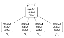
Figure 3: $C_{i}$, $i\in\{2,...,n-1\}$.

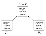
Figure 4: $C_{n}$, terminal configuration.

We consider a star network of $n$ processes ($n\geq 2$): $p_{1}$ is the root of the tree and $p_{2},...,p_{n}$ are the leaves (namely links are $\{\{p_{1},p_{i}\},i=2,...,n\}$). We note $C_{i}$, $i\in\{1,...,n\}$, the configuration satisfying the following three conditions:

• for every $j\in\{1,...,n\}$, $p_{j}.input=1$;

• $p_{1}.sub=i$, for every $j\in\{2,...,i\}$, $p_{j}.sub=1$, and for every $j\in\{i+1,...,n\}$, $p_{j}.sub=0$; and

• for every $j\in\{1,...,n\}$, $p_{j}.res=i$.

$C_{1}$, $C_{i}$ with $i\in\{2,...,n-1\}$, and $C_{n}$ are respectively shown in Figures 4, 4, and 4. In these figures, a variable is underlined whenever an action is enabled to modify it. Note that in configuration $C_{i}$, processes $p_{1}$, …, $p_{i}$ are disabled and processes $p_{i+1},...,p_{n}$ are enabled for $S$. We now build a possible execution that starts from $C_{1}$ and successively converges to configurations $C_{2}$, …, $C_{n}$ ($C_{n}$ is a terminal configuration). To converge from $C_{i}$ to $C_{i+1}$, $i\in\{1,...,n-1\}$, the daemon applies the following scheduling:

1:$p_{i+1}$ executes $S(p_{i+1})$ $\triangleright$ $p_{i+1}.sub=1$

2:$p_{1}$ executes $S(p_{1})$ $\triangleright$ $p_{1}.sub=i+1$

3:$p_{1}$ executes $R(p_{1})$ $\triangleright$ $p_{1}.res=i+1$

4:for $j$$=$$2$ to $n$ do

5:     $p_{j}$ executes $R(p_{j})$ $\triangleright$ $p_{j}.res=i+1$

6:done

For $i\in\{1,...,n-2\}$, the convergence from $C_{i}$ to $C_{i+1}$ lasts exactly one round. Indeed, each process executes at least one action between $C_{i}$ and $C_{i+1}$ and process $p_{n}$ is enabled at configuration $C_{i}$ and remains continuously enabled until being activated as the last process to execute in the round. The convergence from $C_{n-1}$ to $C_{n}$ lasts four rounds: in $C_{n-1}$, only $p_{n}$ is enabled to execute $S(p_{n})$ hence the round terminates in one step where only $S(p_{n})$ is executed. Similarly, $p_{1}$ then sequentially executes $S(p_{1})$ and $R(p_{1})$ in two rounds. Finally, $p_{2},...,p_{n}$ execute $R$ in one round and then the system is in the terminal configuration $C_{n}$.

Hence the above execution lasts $n+3$ rounds.

6 Round Complexity of Algorithms with Acyclic Strategy

In this section, we first propose an extra condition that is sufficient for any algorithm following an acyclic strategy to stabilize in $O(H)$ rounds. We then propose a simple method to add this property to any algorithm that follows an acyclic strategy, without compromising the move complexity.

6.1 A Condition for a Stabilization Time in $O(H)$ rounds

Let $A_{1},...,A_{k}$ be the families’ partition of $\mathcal{A}$. We say that two families $A_{i}$ and $A_{j}$ are locally mutually exclusive if for every process $p$, there is no configuration $\gamma$ where both $A_{i}(p)$ and $A_{j}(p)$ are enabled. By extension, we say $\mathcal{A}$ is locally mutually exclusive if for every $i,j\in\{1,...,k\}$, $i\neq j$ implies that $A_{i}$ and $A_{j}$ are locally mutually exclusive.

Theorem 2.

Let $\mathcal{A}$ be a distributed algorithm for a network $G$ endowed with a spanning forest. If $\mathcal{A}$ follows an acyclic strategy and is locally mutually exclusive, then every execution of $\mathcal{A}$ reaches a terminal configuration within at most $(\mathfrak{H}+1).(H+1)$ rounds, where $\mathfrak{H}$ is the height of the graph of actions’ causality $\mathbf{GC}$ of $\mathcal{A}$ and $H$ is the height of the spanning forest in $G$.

Proof.

Let $A_{i}$ be a family of actions of $\mathcal{A}$ and $p$ be a process. We note $R(A_{i},p)=\mathfrak{H}(A_{i}).(H+1)+M(A_{i},p)+1$ (recall that $\mathfrak{H}(A_{i})$ and $M(A_{i},p)$ are defined in Section 4).

We now show by induction that for every family $A_{i}$ and every process $p$, after $R(A_{i},p)$ rounds $A_{i}(p)$ is disabled forever.

Let $p$ be a process and $A_{i}$ be a family. By definition, $\mathfrak{H}(A_{i})\geq 0$, $H\geq 0$, and $M(A_{i},p)\geq 0$, hence $R(A_{i},p)\geq 1$.

Base Case:

Assume that $R(A_{i},p)=1$. By definition, $M(A_{i},p)=0$ and $\mathfrak{H}(A_{i})=0$. Since $M(A_{i},p)=0$, $Z(p,A_{i})=\{p\}$. So, since $A_{i}$ is top-down or bottom-up, for every $q.v\in G\textit{-Read}(A_{i}(p))$, $q.v\in\textit{Write}(A_{i}(q))\Rightarrow q=p$. Moreover, since $\mathfrak{H}(A_{i})=0$, $\forall j\neq i$, $A_{j}\not\prec_{\mathcal{A}}A_{i}$. So, for every $j\neq i$ and every $q\in p.\Gamma\cup\{p\}$, $\textit{Write}(A_{j}(p))\cap G\textit{-Read}(A_{i}(q))=\emptyset$. Hence, no action except $A_{i}(p)$ can modify a variable in $G\textit{-Read}(A_{i}(p))$. Thus, if $A_{i}(p)$ is (initially) disabled, then $A_{i}(p)$ is disabled forever. Otherwise, $A_{i}(p)$ is continuously enabled until being executed; and, within at most one round, $A_{i}(p)$ is executed since $\mathcal{A}$ is locally mutually exclusive. After this first execution of $A_{i}(p)$, $A_{i}(p)$ is disabled forever since $A_{i}$ is correct-alone.

Induction Hypothesis:

Let $R\geq 1$. Assume that for every family $A_{j}$ and every process $q$ such that $R(A_{j},q)\leq R$, after $R(A_{j},q)$ rounds, $R(A_{j},q)$ is disabled forever.

Induction Step:

Assume that for some family $A_{i}$ and some process $p$, $R(A_{i},p)=R+1$.

Since $A_{i}$ is either bottom-up or top-down and by definition of $\prec_{\mathcal{A}}$, we can deduce that for every family $A_{j}$, every $q\in p.\Gamma\cup\{p\}$, and every $q.v\in\textit{Write}(A_{j}(q))\cap G\textit{-Read}(A_{i}(p))$ one of the following four conditions holds:

1. $j=i\wedge q=p$.

2. $j=i\wedge q\in p.\Gamma\cap Z(p,A_{i})$. In this case, $M(A_{i},q)<M(A_{i},p)$, so $R(A_{i},q)<R(A_{i},p)=R+1$.

3. $j\neq i\wedge q=p\wedge A_{j}\prec_{\mathcal{A}}A_{i}$. In this case, $A_{j}\prec_{\mathcal{A}}A_{i}$ implies that $\mathfrak{H}(A_{j})<\mathfrak{H}(A_{i})$, so $R(A_{j},q)=R(A_{j},p)<R(A_{i},p)=R+1$.

4. $j\neq i\wedge q\in p.\Gamma\wedge A_{j}\prec_{\mathcal{A}}A_{i}$. In this case, $A_{j}\prec_{\mathcal{A}}A_{i}$ implies that $\mathfrak{H}(A_{j})<\mathfrak{H}(A_{i})$. Moreover, $M(A_{j},q)-M(A_{i},p)\leq H$. So, $R(A_{j},q)<R(A_{i},p)=R+1$.

Thus, by induction hypothesis, after $R$ rounds, all variables of $G\textit{-Read}(A_{i}(p))$ satisfying Cases (2), (3), or (4) are constant forever, i.e., all variables of $G\textit{-Read}(A_{i}(p))$, except maybe those written by $A_{i}(p)$ itself (Case (1)), are constant forever. So, if after $R$ rounds, $A_{i}(p)$ is disabled, then it is disabled forever. Otherwise, after $R$ rounds, $A_{i}(p)$ is continuously enabled until being executed; and, within at most one additional round, $A_{i}(p)$ is executed since $\mathcal{A}$ is locally mutually exclusive. After the execution of $A_{i}(p)$, $A_{i}(p)$ is disabled forever since $A_{i}$ is correct-alone. Hence, after $R+1$ rounds, $A_{i}(p)$ is disabled forever, and we are done.

Since for every family $A_{i}$ and every process $p$, $\mathfrak{H}(A_{i})\leq\mathfrak{H}$ and $M(A_{i},p)\leq H$, we have $R(A_{i},p)\leq(\mathfrak{H}+1).(H+1)$, hence the lemma holds. ∎

From Theorem 2 and Definition 1, follows.

Corollary 2.

Let $\mathcal{A}$ be a distributed algorithm for a network $G$ endowed with a spanning forest and $SP$ a predicate over the configurations of $\mathcal{A}$. If $\mathcal{A}$ follows an acyclic strategy, is locally mutually exclusive, and every terminal configuration of $\mathcal{A}$ satisfies $SP$, then

• $\mathcal{A}$ is silent and self-stabilizing for $SP$ in $G$ under the distributed unfair daemon, and

• its stabilization time is at most $(\mathfrak{H}+1).(H+1)$ rounds,

where $\mathfrak{H}$ the height of the graph of actions’ causality $\mathbf{GC}$ of $\mathcal{A}$ and $H$ is the height of the spanning forest in $G$.

By definition, $\mathfrak{H}<k$, the bound exhibited by the previous lemma is in $O(k.H)$ where $k$ is the number of families of the algorithm. Actually, the local mutual exclusion of the algorithm is usually implemented by enforcing priorities on families as in the transformer presented below. Hence, in practical cases, $\mathfrak{H}=k-1$, as shown in Lemma 8.

6.2 A Transformer

We have shown in Subsection 5.2 that there exist algorithms that follow an acyclic strategy, are not locally mutually exclusive and stabilize in $\Omega(n)$ rounds in the worst case. So, we formalize now a generic method based on priorities over actions to give the mutually exclusive property to such algorithms; this ensures a complexity in $O(H)$ rounds. Notice that the method does not degrade the move complexity.

Let $\mathcal{A}$ be any distributed algorithm for a network $G$ endowed with a spanning forest that follows an acyclic strategy. Let $k$ be the number of families of $\mathcal{A}$. In the following, for every process $p$ and every family $A_{i}$, we identify the guard and the statement of Action $A_{i}(p)$ by $G_{i}(p)$ and $S_{i}(p)$, respectively.

Let $\triangleleft_{\mathcal{A}}$ be any strict total order on families of $\mathcal{A}$ compatible with $\prec_{\mathcal{A}}$, i.e., $\triangleleft_{\mathcal{A}}$ is a binary relation on families of $\mathcal{A}$ that satisfies the following three conditions:

Strict Order:

$\triangleleft_{\mathcal{A}}$ is irreflexive and transitive;

Total:

for every two families $A_{i},A_{j}$, we have either $A_{i}\triangleleft_{\mathcal{A}}A_{j}$, $A_{j}\triangleleft_{\mathcal{A}}A_{i}$, or $i=j$; and

Compatibility:

for every two families $A_{i},A_{j}$, if $A_{i}\prec_{\mathcal{A}}A_{j}$, then $A_{i}\triangleleft_{\mathcal{A}}A_{j}$.

Let ${\tt T}(\mathcal{A})$ be the following algorithm:

• ${\tt T}(\mathcal{A})$ and $\mathcal{A}$ have the same set of variables.

• Every process $p\in V$ holds the following $k$ actions. For every $i\in\{1,...,k\}$,

  $$A^{\tt T}_{i}(p)\ ::\ G_{i}^{\tt T}(p)\ \longmapsto\ S_{i}^{\tt T}(p)$$

  where $G_{i}^{\tt T}(p)=\big{(}\bigwedge_{A_{j}\triangleleft_{\mathcal{A}}A_{i}}\neg G_{j}(p)\big{)}\wedge G_{i}(p)$ and $S_{i}^{\tt T}(p)=S_{i}(p)$.

  $G_{i}(p)$ (resp. the set $\{G_{j}(p)\ :\ A_{j}\triangleleft_{\mathcal{A}}A_{i}\}$) is called the positive part (resp. negative part) of $G^{\tt T}_{i}(p)$.

Notice that, by definition, $\prec_{\mathcal{A}}$ is irreflexive and the graph of actions’ causality induced by $\prec_{\mathcal{A}}$ is acyclic. Hence, there always exists a strict total order compatible with $\prec_{\mathcal{A}}$, i.e., the above transformation is always possible for any algorithm $\mathcal{A}$ which follows an acyclic strategy.

Remark 5.

${\tt T}(\mathcal{A})$ is well-formed and $A^{\tt T}_{1},...,A^{\tt T}_{k}$ is the families’ partition of ${\tt T}(\mathcal{A})$, where $A^{\tt T}_{i}=\{A^{\tt T}_{i}(p)\ :\ p\in V\}$, for every $i\in\{1,...,k\}$.

By construction, we have :

Remark 6.

For every $i,j\in\{1,...,k\}$ such that $i\neq j$, and every process $p$, the positive part of $G_{j}^{\tt T}(p)$ belongs to the negative part in $G_{i}^{\tt T}(p)$ if and only if $A_{j}\triangleleft_{\mathcal{A}}A_{i}$.

Lemma 4.

${\tt T}(\mathcal{A})$ is locally mutually exclusive.

Proof.

Let $A_{i}^{\tt T}$ and $A_{j}^{\tt T}$ be two different families of ${\tt T}(\mathcal{A})$. Then, either $A_{i}\triangleleft_{\mathcal{A}}A_{j}$ or $A_{j}\triangleleft_{\mathcal{A}}A_{i}$ ($\triangleleft_{\mathcal{A}}$ is a strict total order). Without the loss of generality, assume $A_{i}\triangleleft_{\mathcal{A}}A_{j}$. Let $p$ be any process and $\gamma$ be any configuration. The positive part of $G_{i}^{\tt T}(p)$ belongs to the negative part of $G_{j}^{\tt T}(p)$ (see Remark 6), and consequently, $A_{i}^{\tt T}(p)$ and $A_{j}^{\tt T}(p)$ cannot be both enabled in $\gamma$. Hence, $A_{i}^{\tt T}$ and $A_{j}^{\tt T}$ are locally mutually exclusive, which in turns implies that ${\tt T}(\mathcal{A})$ is locally mutually exclusive. ∎

Lemma 5.

For every $i,j\in\{1,...,k\}$, if $A^{\tt T}_{j}\prec_{{\tt T}(\mathcal{A})}A^{\tt T}_{i}$, then $A_{j}\triangleleft_{\mathcal{A}}A_{i}$.

Proof.

Let $A_{i}^{\tt T}$ and $A_{j}^{\tt T}$ be two families such that $A^{\tt T}_{j}\prec_{{\tt T}(\mathcal{A})}A^{\tt T}_{i}$. Then, $i\neq j$ and there exist two processes $p$ and $q$ such that $q\in p.\Gamma\cup\{p\}$ and $\textit{Write}(A^{\tt T}_{j}(p))\cap G\textit{-Read}(A^{\tt T}_{i}(q))\neq\emptyset$. Then, $\textit{Write}(A^{\tt T}_{j}(p))=\textit{Write}(A_{j}(p))$, and either $\textit{Write}(A_{j}(p))\cap G\textit{-Read}(A_{i}(q))\neq\emptyset$, or $\textit{Write}(A_{j}(p))\cap G\textit{-Read}(A_{k}(q))\neq\emptyset$ where $G_{k}(q)$ belongs to the negative part of $G^{\tt T}_{i}(q)$. In the former case, we have $A_{j}\prec_{\mathcal{A}}A_{i}$, which implies that $A_{j}\triangleleft_{\mathcal{A}}A_{i}$ ($\triangleleft_{\mathcal{A}}$ is compatible with $\prec_{\mathcal{A}}$). In the latter case, $A_{j}\prec_{\mathcal{A}}A_{k}$ (by definition) and $A_{k}\triangleleft_{\mathcal{A}}A_{i}$ (by Remark 6). Since, $A_{j}\prec_{\mathcal{A}}A_{k}$ implies $A_{j}\triangleleft_{\mathcal{A}}A_{k}$ ($\triangleleft_{\mathcal{A}}$ is compatible with $\prec_{\mathcal{A}}$), by transitivity we have $A_{j}\triangleleft_{\mathcal{A}}A_{i}$. Hence, for every $i,j\in\{1,...,k\}$, $A^{\tt T}_{j}\prec_{{\tt T}(\mathcal{A})}A^{\tt T}_{i}$ implies $A_{j}\triangleleft_{\mathcal{A}}A_{i}$, and we are done. ∎

Lemma 6.

${\tt T}(\mathcal{A})$ follows an acyclic strategy.

Proof.

Let $A_{i}^{\tt T}$ be a family of ${\tt T}(\mathcal{A})$. The lemma is immediate from the following three claims.

Claim I:

$A_{i}^{\tt T}$ is correct-alone.

Proof of the claim: Since $\mathcal{A}$ follows an acyclic strategy, $A_{i}$ is correct-alone. Moreover, for every process $p$, we have $S_{i}^{\tt T}(p)=S_{i}(p)$ and $\neg G_{i}(p)\Rightarrow\neg G_{i}^{\tt T}(p)$. Hence, $A_{i}^{\tt T}$ is also correct-alone.

Claim II:

$A_{i}^{\tt T}$ is either bottom-up or top-down.

Proof of the claim: Since $\mathcal{A}$ follows an acyclic strategy, $A_{i}$ is either bottom-up or top-down. Assume $A_{i}$ is bottom-up. By construction, for every process $q$, $S_{i}^{\tt T}(q)=S_{i}(q)$, which implies that $\textit{Write}(A^{\tt T}_{i}(q))=\textit{Write}(A_{i}(q))$. Let $q.v\in G\textit{-Read}(A^{\tt T}_{i}(p))$.

• Assume $q.v\in G\textit{-Read}(A_{i}(p))$. Then $q.v\in\textit{Write}(A_{i}(q))\Rightarrow q\in p.children\cup\{p\}$ (since $A_{i}$ is bottom-up), i.e., $q.v\in\textit{Write}(A^{\tt T}_{i}(q))\Rightarrow q\in p.children\cup\{p\}$.

• Assume now that $q.v\notin G\textit{-Read}(A_{i}(p))$. Then $q.v\in G\textit{-Read}(A_{j}(p))$ such that $G_{j}(p)$ belongs to the negative part of $G^{{\tt T}}_{i}(p)$, i.e., $A_{j}\triangleleft_{\mathcal{A}}A_{i}$ (Remark 6). Assume, by the contradiction, that $q.v\in\textit{Write}(A^{\tt T}_{i}(q))$. Then $q.v\in\textit{Write}(A_{i}(q))$, and since $p\in q.\Gamma\cup\{q\}$ (indeed, $q.v\in G\textit{-Read}(A_{j}(p))$), we have $A_{i}\prec_{\mathcal{A}}A_{j}$. Now, as $\triangleleft_{\mathcal{A}}$ is compatible with $\prec_{\mathcal{A}}$, we have $A_{i}\triangleleft_{\mathcal{A}}A_{j}$. Hence, $A_{j}\triangleleft_{\mathcal{A}}A_{i}$ and $A_{i}\triangleleft_{\mathcal{A}}A_{j}$, a contradiction. Thus, $q.v\notin\textit{Write}(A^{\tt T}_{i}(q))$ which implies that $q.v\in\textit{Write}(A^{\tt T}_{i}(q))\Rightarrow q\in p.children\cup\{p\}$ holds in this case.

Hence, $A_{i}^{\tt T}$ is bottom-up.

Following a similar reasoning, if $A_{i}$ is top-down, we can show $A_{i}^{\tt T}$ is top-down too.

Claim III:

The graph of actions’ causality of ${\tt T}(\mathcal{A})$ is acyclic.

Proof of the claim: By Lemma 5, for every $i,j\in\{1,...,k\}$, $A^{\tt T}_{j}\prec_{{\tt T}(\mathcal{A})}A^{\tt T}_{i}\Rightarrow A_{j}\triangleleft_{\mathcal{A}}A_{i}$. Now, $\triangleleft_{\mathcal{A}}$ is a strict total order. So, the graph of actions’ causality of ${\tt T}(\mathcal{A})$ is acyclic.

∎

Lemma 7.

Every execution of ${\tt T}(\mathcal{A})$ is an execution of $\mathcal{A}$.

Proof.

The lemma is immediate from the following three claims.

Claim I:

$\mathcal{A}$ and ${\tt T}(\mathcal{A})$ have the same set of configurations.

Proof of the claim: By definition.

Claim II:

Every step of ${\tt T}(\mathcal{A})$ is a step of $\mathcal{A}$.

Proof of the claim: $G_{i}(p)$ is the guard of $A_{i}(p)$ and the positive part of $G^{\tt T}_{i}(p)$. So, $G^{{\tt T}}_{i}(p)$ implies $G_{i}(p)$, i.e., if $A^{\tt T}_{i}(p)$ is enabled, then $A_{i}(p)$ is enabled. Since $S_{i}^{\tt T}(p)=S_{i}(p)$, we are done.

Claim III:

Let $\gamma$ be any configuration. $\gamma$ is terminal w.r.t. ${\tt T}(\mathcal{A})$ if and only if $\gamma$ is terminal w.r.t. $\mathcal{A}$.

Proof of the claim: $\gamma$ is terminal w.r.t. ${\tt T}(\mathcal{A})$ if and only if

$$\bigwedge_{p\in V}\bigwedge_{i\in\{1,...,k\}}\neg G_{i}^{\tt T}(p) =\bigwedge_{p\in V}\bigwedge_{i\in\{1,...,k\}}\neg\big{(}\big{(}\bigwedge_{A_{j}\triangleleft_{\mathcal{A}}A_{i}}\neg G_{j}(p)\big{)}\wedge G_{i}(p)\big{)}$$

$$=\bigwedge_{p\in V}\bigwedge_{i\in\{1,...,k\}}\big{(}\big{(}\bigvee_{A_{j}\triangleleft_{\mathcal{A}}A_{i}}G_{j}(p)\big{)}\vee\neg G_{i}(p)\big{)}$$

$$=\bigwedge_{p\in V}\bigwedge_{i\in\{1,...,k\}}\neg G_{i}(p)$$

Now, $\bigwedge_{p\in V}\bigwedge_{i\in\{1,...,k\}}\neg G_{i}(p)$ if and only if $\gamma$ is terminal w.r.t. $\mathcal{A}$.

∎

Theorem 3.

Let $\mathcal{A}$ be a distributed algorithm for a network $G$ endowed with a spanning forest, $SP$ a predicate over the configurations of $\mathcal{A}$. If $\mathcal{A}$ follows an acyclic strategy, and is silent and self-stabilizing for $SP$ in $G$ under the distributed unfair daemon, then

1. ${\tt T}(\mathcal{A})$ is silent and self-stabilizing for $SP$ in $G$ under the distributed unfair daemon,

2. its stabilization time is at most $(\mathfrak{H}+1).(H+1)$ rounds, and

3. its stabilization time in moves is less than or equal to the one of $\mathcal{A}$.

where $\mathfrak{H}$ is the height of the graph of actions’ causality $\mathbf{GC}$ of $\mathcal{A}$ and $H$ is the height of the spanning forest in $G$.

Proof.

(1) and (3) are consequences of Lemma 7 and Corollary 2. (2) follows from Lemmas 4, 6, and Theorem 2. ∎

Using the above theorem, our toy example $\mathcal{TE}$ stabilizes in at most $2(H+1)$ rounds, keeping a move complexity in $\Theta(H.n^{2})$ in the worst case (recall that the worst-case execution of $\mathcal{TE}$ proposed in Subsection 5.1 is also a possible execution of ${\tt T}(\mathcal{TE})$).

The next lemma shows that in usual cases, the height $\mathfrak{H}$ of graph of actions’ causality of ${\tt T}(\mathcal{A})$ satisfies $\mathfrak{H}=k-1$, where $k$ is the number of families of $\mathcal{A}$.

Lemma 8.

If for every $i\in\{1,...,k\}$ and every $p\in V$, $G_{i}(p)\not\equiv false$, then

for every $x,y\in\{1,...,k\}$, $A^{\tt T}_{x}\prec_{{\tt T}(\mathcal{A})}A^{\tt T}_{y}$ if and only if $A_{x}\triangleleft_{\mathcal{A}}A_{y}$.

Consequently, the height $\mathfrak{H}$ of graph of actions’ causality of ${\tt T}(\mathcal{A})$ satisfies $\mathfrak{H}=k-1$ (indeed $\triangleleft_{\mathcal{A}}$ is a strict total order).

Proof.

Let $x,y\in\{1,...,k\}$. By Lemma 5, $A^{\tt T}_{x}\prec_{{\tt T}(\mathcal{A})}A^{\tt T}_{y}\Rightarrow A_{x}\triangleleft_{\mathcal{A}}A_{y}$. Assume now that $A_{x}\triangleleft_{\mathcal{A}}A_{y}$. By irreflexivity, $x\neq y$. Let $p$ be any process. Since $A_{x}$ is correct-alone and $G_{x}(p)\not\equiv false$, $\textit{Write}(A_{x}(p))\cap G\textit{-Read}(A_{x}(p))\neq\emptyset$. Now, $G_{x}(p)$ belongs to the negative part of $A^{\tt T}_{y}$ (Remark 6) and $\textit{Write}(A^{{\tt T}}_{x}(p))=\textit{Write}(A_{x}(p))$. So, $\textit{Write}(A^{{\tt T}}_{x}(p))\cap G\textit{-Read}(A^{\tt T}_{y}(p))\neq\emptyset$. Hence, $A^{\tt T}_{x}\prec_{{\tt T}(\mathcal{A})}A^{\tt T}_{y}$, and we are done. ∎

7 Related Work and Applications

In this section, we review some existing works from the literature and show how to apply our generic results on them. Those works propose silent self-stabilizing algorithms for directed trees or network where a directed spanning tree is available. These algorithms are, or can be easily translated into, well-formed algorithms that follow an acyclic strategy. Hence, their correctness and time complexities (in moves and rounds) are directly deduced from our results.

A Distributed Algorithm for Minimum Distance-$k$ Domination in Trees [9].

This paper proposes three algorithms for directed trees. Each algorithm is given with its proof of correctness and round complexity, however move complexity is not considered. Our results allow to obtain the same round complexities, and additionally provide move complexities.

The first algorithm converges to a legitimate terminal configuration where a minimum distance-$k$ dominating set is defined. This algorithm can be trivially translated in our model as an algorithm with a single variable and a single action at each process $p$,

$$A_{1}(p)::p.L\neq\mathcal{L}(p)\longmapsto p.L\leftarrow\mathcal{L}(p)$$

We do not explain here the algorithm, for the role of variable $L$ and its computation using $\mathcal{L}(p)$, please refer to the original paper [9]. Now, from the definition of $\mathcal{L}$ in [9], we know that $\mathcal{L}(p)$ depends on $q.L$ for $q\in p.children$; hence the family $A_{1}$ is bottom-up and correct-alone. Thus, we can deduce from our results that the translation of this algorithm in our model is silent and self-stabilizing with a stabilization time in $O(H)$ rounds (Theorem 2) and $O(n^{2})$ moves (Theorem 1) where $H$ is the height of the tree and $n$ is the number of processes.

The second algorithm is an extension of the first one since it computes both a minimum distance-$k$ dominating set and a maximum distance-$2k$ independent set. This algorithm is made of two families of actions $A_{1}$ and $A_{2}$: for every node $p$,

$$A_{1}(p)::p.L\neq\mathcal{L}(p)\longmapsto p.L\leftarrow\mathcal{L}(p)$$

$$A_{2}(p)::p.fading\neq fading(p)\longmapsto p.fading\leftarrow fading(p)$$

We already know that $A_{1}$ is bottom-up and correct-alone. Then, from the definitions given in [9], we can easily deduce that $A_{2}$ is top-down and correct-alone since $fading(p)$ depends on $p.parent.fading$ and $q.L$ with $q\in p.children$, which is not written by the family $A_{2}$. Hence, the graph of actions’ causality is

$$A_{1}\longrightarrow A_{2}$$

Thus, we obtain a stabilization time of $O(H)$ rounds (as in [9]), but additionally we obtain a move complexity in $O(n^{2}.H)$.

The third algorithm computes minimum connected distance-$k$ dominating sets using five families of actions $A_{1},...,A_{5}$:

$$A_{1}(p)::p.L\neq\mathcal{L}(p)\longmapsto p.L\leftarrow\mathcal{L}(p)$$

$$A_{2}(p)::p.level\neq level(p)\longmapsto p.level\leftarrow level(p)$$

$$A_{3}(p)::p.cds\neq cds^{\prime}(p)\longmapsto p.cds\leftarrow cds^{\prime}(p)$$

$$A_{4}(p)::p.cds\wedge p.dist_{l}\neq dist_{l}(p)\longmapsto p.dist_{l}\leftarrow dist_{l}(p)$$

$$A_{5}(p)::p.minc\neq minc(p)\longmapsto p.minc\leftarrow minc(p)$$

From [9]:

• $\mathcal{L}(p)$ depends on $q.L$ for $q\in p.children$,

• $level(p)$ depends on $p.parent.level$,

• we note $cds^{\prime}(p)=\texttt{if }p.L=k\texttt{ then }true\texttt{ else }cds(p)$ and $cds(p)$ depends on $q.cds$ for $q\in p.children$,

• $dist_{l}(p)$ depends on $q.L$ and $q.cds$ for $q\in p.children$, and $p.parent.dist_{l}$,

• $minc(p)$ depends on $p.level$, $q.cds$ and $q.minc$ for $q\in p.children$.

Hence $A_{1},A_{3},A_{5}$ are bottom-up and correct-alone and $A_{2},A_{4}$ are top-down and correct-alone. The graph of actions’ causality is acyclic since $A_{1}\prec A_{3}$, $A_{1}\prec A_{4}$, $A_{2}\prec A_{5}$, $A_{3}\prec A_{4}$, and $A_{3}\prec A_{5}$; and its height is $\mathfrak{H}=2$. Thus, conformly to [9], we obtain a round complexity in $O(H)$. Moreover, Theorem 1 provides a move complexity in $O(\Delta^{2}.n^{4})$ (with $\Delta$ the degree of the tree).

Self-stabilizing Tree Ranking [35].

In this paper, the authors propose a silent self-stabilizing algorithm that works on a directed tree and computes various rankings of the processes following several kind of tree traversals such as pre-order or breadth-first traversal, assuming a central unfair daemon. They assume that each node knows a predefined order on its children so that the traversal ordering is deterministic.

Following our method, the proposed algorithm is made of six families of actions.

• $A_{1}$ computes $D$, the number of proper descendants of the process, it also copies the number of proper descendants of each of children of the process. This family is bottom-up and correct-alone.

• $A_{2}$ computes $L$, the level of the node. This family is top-down and correct-alone.

• $A_{3}$ computes $PRE$, the preorder rank of the node. The value of $PRE$ depends on values computed by $A_{1}$, so $A_{3}$ is top-down and correct-alone. $A_{3}$ also computes $LABEL$, which is an intermediate labelling used for breadth-first ranking, $LABEL$ directly depends on the values of $L$ and $PRE$ of the process.

• $A_{4}$ computes $POST$ and $RPOST$, the postorder and preorder ranks of the process. The values of $POST$ and $RPOST$ depend on values computed by $A_{1}$, so $A_{4}$ is top-down and correct-alone.

• $A_{5}$ computes $DLIST$ (an intermediate list of nodes for breadth-first ranking) in a bottom-up and correct-alone manner, since the value of $DLIST$ depends on $LABEL$ at the node and $DLIST$ at the children of the process.

• $A_{6}$ computes $RLIST$ (the list of all nodes in the breadth-first order) and $BFR$ the breadth-first rank of the process. $A_{6}$ is top-down and correct-alone since the values written by $A_{6}$ depend on $RLIST$ at the process and its parent as well as $DLIST$ and $LABEL$ at the process.

In [35], the authors divide the algorithm in two phases: in phase 1, actions $A_{1}$ and $A_{2}$ are executed and converge and then, after global termination of phase 1, phase 2 begins with the other actions from $A_{3}$ to $A_{6}$. But our results apply: there is no need to separate those two phases and the full algorithm is silent and self-stabilizing under an unfair distributed daemon. Note that the fact that after termination, we have correct tree rankings is proven in the original paper. Moreover, note that we extend this result since it has been proven for a central unfair daemon only. For round complexity, we obtain $O(H)$ rounds, like in the original paper. For move complexity, we obtain $O(\Delta^{3}.n^{5})$ moves using an unfair distributed daemon, while the authors obtain $O(n^{2})$ moves using an unfair central daemon and assuming the computation is divided in two separated phases. Note that the overhead we obtain is not surprising since centrality and phase separation remove any interleaving.

Improved Self-Stabilizing Algorithms for L(2, 1)-Labeling Tree Networks [8].

In [8], the authors propose two silent self-stabilizing algorithms for computing a particular labelling in directed trees. Although more simple, their solutions follows the same ideas as in [35]: each algorithm contains a single family of actions which is correct-alone and top-down. We obtain the same bounds as in [35], namely the two algorithms are silent self-stabilizing under a distributed unfair daemon and converge within $O(n.H)$ moves and $O(H)$ rounds.

An $O(n^{2})$ Self-Stabilizing Algorithm for Computing Bridge-Connected Components [36]

In [36], an algorithm is proposed to compute bridge-connected components in a network endowed with a depth-first spanning tree. The algorithm is proven to be silent self-stabilizing under an unfair distributed daemon. However, as in [35], it is separated into two phases, the first phase has to be finished, globally, before the second phase begins. The first phase corresponds to one family of actions (that computes variable $S$) which are correct-alone and bottom-up, while the second phase corresponds to a second family of actions (to compute variable $BCC$) which is correct-alone and top-down. Our results show the correctness of the algorithm without enforcing those phases, with a stabilization time in $O(n^{3})$ moves and $O(H)$ rounds, respectively. Note that the original paper does not provide the round complexity and obtains $O(n^{2})$ moves in case the two phases are executed in sequence without any interleaving.

A Note on Self-Stabilizing Articulation Point Detection [37].

This paper proposes a silent self-stabilizing solution for articulation point detection in a network endowed with a depth-first spanning tree. The algorithm is exactly the first phase of [36], i.e., a single family of correct-alone and bottom-up actions. It converges in at most $O(n^{2})$ moves and $O(H)$ rounds under an unfair distributed daemon.

A Self-Stabilizing Algorithm for Finding Articulation Points [38].

The silent algorithm given in [38] finds articulation points in a network endowed with a breadth-first spanning tree, assuming a central unfair daemon. The algorithm computes for each node $p$ the variable $p.e$ which contains every non-tree edges incident on $p$ and some non-tree edges incident on descendants of $p$ once a terminal configuration has been reached. Precisely, a non-tree edge $\{p,q\}$ is propagated up in the tree starting from $p$ and $q$ until the first common ancestor of $p$ and $q$. Based on $p.e$, the node $p$ can decide whether or not it is an articulation point. The algorithm can be translated in our model as a single family of actions which is correct-alone and bottom-up. From our results, it follows that this algorithm is actually silent and self-stabilizing even assuming a distributed unfair daemon. Moreover, its stabilization time is in $O(n^{2})$ moves and $O(H)$ rounds, respectively.

A Self-Stabilizing Algorithm for Bridge Finding [39].

The algorithm in [39] computes bridges in a network endowed with a breadth-first spanning tree, assuming a distributed unfair daemon. As in [38], the algorithm computes a variable $p.s$ at each node $p$ using a single family which is correct-alone and bottom-up. The correctness of this algorithm assuming a distributed unfair daemon is direct from our results. Moreover, we obtain a stabilization time in $O(n^{2})$ moves and $O(H)$ rounds.

A Silent Self-stabilizing Algorithm for Finding Cut-Nodes and Bridges [40].

The algorithm in [40] computes cut-nodes and bridges on connected graph endowed with a depth-first spanning tree. It is silent and self-stabilizing under a distributed unfair distributed daemon and converges within $O(n^{2})$ moves and $O(H)$ rounds, respectively. Indeed, the algorithm contains a single family of actions which is correct-alone and bottom-up.

8 Conclusion

We have presented a general scheme to prove and analyze silent self-stabilizing algorithms running on networks endowed with a sense of direction describing a spanning forest. Our results allow to easily (i.e. quasi-syntactically) deduce upper bounds on move and round complexities of such algorithms. We have shown, using a toy example, that our method allow to easily obtain tight complexity bounds, precisely a stabilization time which is asymptotically optimal in rounds and polynomial in moves. Finally, we reviewed a number of existing silent self-stabilizing solutions from the literature [9, 35, 8, 36, 37, 38, 40] where our method applies. In some of them, we were able to provide more general results than those proven in the original papers. Namely, some algorithms are proven using a strong daemon, whereas our work extends to the most general daemon assumption, i.e., the distributed unfair daemon. Moreover, many papers only focus on one kind of time complexity measure, whereas our results systematically provide round as well as move complexities.

In many of those related works, the assumption about the existence of a directed (spanning) tree in the network has to be considered as an intermediate assumption, since this structure has to be built by an underlying algorithm. Now, there are several silent self-stabilizing spanning tree constructions that are efficient in both rounds and moves, e.g., [32]. Thus, both algorithms, i.e., the one that builds the tree and the one that computes on this tree, have to be carefully composed to obtain a general composite algorithm where, the stabilization time is keeped both asymptotically optimal in rounds and polynomial in moves.

References

- [1] Edsger W. Dijkstra. Self-stabilizing systems in spite of distributed control. Communications of the ACM, 17(11):643–644, 1974.
- [2] L. Blin, M. Potop-Butucaru, S. Rovedakis, and S. Tixeuil. Loop-free super-stabilizing spanning tree construction. In the 12th International Symposium on Stabilization, Safety, and Security of Distributed Systems (SSS’10), Springer LNCS 6366, pages 50–64, 2010.
- [3] Shing-Tsaan Huang and Nian-Shing Chen. Self-stabilizing depth-first token circulation on networks. Distributed Computing, 7(1):61–66, 1993.
- [4] Jean-Michel Couvreur, Nissim Francez, and Mohamed G. Gouda. Asynchronous unison (extended abstract). In the 12th International Conference on Distributed Computing Systems (ICDCS’92), pages 486–493. IEEE Computer Society, 1992.
- [5] Alain Bui, Ajoy Kumar Datta, Franck Petit, and Vincent Villain. Optimal PIF in tree networks. In the 2nd International Meeting on Distributed Data & Structures 2 (WDAS 1999), pages 1–16, 1999.
- [6] Toshimitsu Masuzawa and Hirotsugu Kakugawa. Self-stabilization in spite of frequent changes of networks: Case study of mutual exclusion on dynamic rings. In Ted Herman and Sébastien Tixeuil, editors, Self-Stabilizing Systems, 7th International Symposium, SSS 2005, Barcelona, Spain, October 26-27, 2005, Proceedings, volume 3764 of Lecture Notes in Computer Science, pages 183–197. Springer, 2005.
- [7] Lélia Blin and Sébastien Tixeuil. Compact deterministic self-stabilizing leader election on a ring: the exponential advantage of being talkative. Distributed Computing, 31(2):139–166, 2018.
- [8] Pranay Chaudhuri and Hussein Thompson. Improved self-stabilizing algorithms for l(2, 1)-labeling tree networks. Mathematics in Computer Science, 5(1):27–39, 2011.
- [9] Volker Turau and Sven Köhler. A distributed algorithm for minimum distance-k domination in trees. J. Graph Algorithms Appl., 19(1):223–242, 2015.
- [10] Ji-Cherng Lin and Ming-Yi Chiu. A fault-containing self-stabilizing algorithm for 6-coloring planar graphs. J. Inf. Sci. Eng., 26(1):163–181, 2010.
- [11] Sukumar Ghosh and Mehmet Hakan Karaata. A self-stabilizing algorithm for coloring planar graphs. Distributed Computing, 7(1):55–59, 1993.
- [12] Ajoy Kumar Datta, Shivashankar Gurumurthy, Franck Petit, and Vincent Villain. Self-stabilizing network orientation algorithms in arbitrary rooted networks. Stud. Inform. Univ., 1(1):1–22, 2001.
- [13] Karine Altisen, Alain Cournier, Stéphane Devismes, Anaïs Durand, and Franck Petit. Self-stabilizing leader election in polynomial steps. Inf. Comput., 254:330–366, 2017.
- [14] G Tel. Introduction to distributed algorithms. Cambridge University Press, Cambridge, UK, Second edition 2001.
- [15] A Arora, MG Gouda, and T Herman. Composite routing protocols. In the 2nd IEEE Symposium on Parallel and Distributed Processing (SPDP’90), pages 70–78, 1990.
- [16] Ajoy Kumar Datta, Stéphane Devismes, Karel Heurtefeux, Lawrence L. Larmore, and Yvan Rivierre. Competitive self-stabilizing k-clustering. Theor. Comput. Sci., 626:110–133, 2016.
- [17] Shlomi Dolev, Mohamed G. Gouda, and Marco Schneider. Memory requirements for silent stabilization. Acta Informatica, 36(6):447–462, 1999.
- [18] Fabienne Carrier, Ajoy Kumar Datta, Stéphane Devismes, Lawrence L. Larmore, and Yvan Rivierre. Self-stabilizing (f, g)-alliances with safe convergence. J. Parallel Distrib. Comput., 81-82:11–23, 2015.
- [19] Ajoy K. Datta, Lawrence L. Larmore, and Priyanka Vemula. An o(n)-time self-stabilizing leader election algorithm. jpdc, 71(11):1532–1544, 2011.
- [20] Ajoy Kumar Datta, Lawrence L. Larmore, and Priyanka Vemula. Self-stabilizing leader election in optimal space under an arbitrary scheduler. Theoretical Computer Science, 412(40):5541–5561, 2011.
- [21] Christian Glacet, Nicolas Hanusse, David Ilcinkas, and Colette Johnen. Disconnected components detection and rooted shortest-path tree maintenance in networks. In the 16th International Symposium on Stabilization, Safety, and Security of Distributed Systems (SSS’14), Springer LNCS 8736, pages 120–134, 2014.
- [22] Shing-Tsaan Huang and Nian-Shing Chen. A self-stabilizing algorithm for constructing breadth-first trees. Information Processing Letters, 41(2):109–117, 1992.
- [23] Stéphane Devismes and Colette Johnen. Silent self-stabilizing {BFS} tree algorithms revisited. Journal of Parallel and Distributed Computing, 97:11 – 23, 2016.
- [24] Christian Glacet, Nicolas Hanusse, David Ilcinkas, and Colette Johnen. Disconnected components detection and rooted shortest-path tree maintenance in networks - extended version. Technical report, LaBRI, CNRS UMR 5800, 2016.
- [25] Shmuel Katz and Kenneth J. Perry. Self-stabilizing extensions for message-passing systems. Distributed Computing, 7(1):17–26, 1993.
- [26] Paolo Boldi and Sebastiano Vigna. Universal dynamic synchronous self–stabilization. Distributed Computing, 15(3):137–153, July 2002.
- [27] Bertrand Ducourthial and Sébastien Tixeuil. Self-stabilization with r-operators. Distributed Computing, 14(3):147–162, 2001.
- [28] Sylvie Delaët, Bertrand Ducourthial, and Sébastien Tixeuil. Self-stabilization with r-operators revisited. Journal of Aerospace Computing, Information, and Communication (JACIC), 3(10):498–514, 2006.
- [29] Lélia Blin, Pierre Fraigniaud, and Boaz Patt-Shamir. On proof-labeling schemes versus silent self-stabilizing algorithms. In 16th International Symposium on Stabilization, Safety, and Security of Distributed Systems (SSS 2014), Springer LNCS 8756, pages 18–32, 2014.
- [30] Amos Korman, Shay Kutten, and David Peleg. Proof labeling schemes. Distributed Computing, 22(4):215–233, 2010.
- [31] Alain Cournier, Stéphane Devismes, and Vincent Villain. Light enabling snap-stabilization of fundamental protocols. TAAS, 4(1):6:1–6:27, 2009.
- [32] Stéphane Devismes, David Ilcinkas, and Colette Johnen. Silent Self-Stabilizing Scheme for Spanning-Tree-like Constructions. Technical report, HAL, February 2018.
- [33] S Dolev, A Israeli, and S Moran. Self-stabilization of dynamic systems assuming only Read/Write atomicity. Distributed Computing, 7(1):3–16, 1993.
- [34] Shlomi Dolev, Mohamed G. Gouda, and Marco Schneider. Memory requirements for silent stabilization. Acta Inf., 36(6):447–462, 1999.
- [35] Pranay Chaudhuri and Hussein Thompson. Self-stabilizing tree ranking. Int. J. Comput. Math., 82(5):529–539, 2005.
- [36] Pranay Chaudhuri. An Self-Stabilizing Algorithm for Computing Bridge-Connected Components. Computing, 62(1):55–67, 1999.
- [37] Pranay Chaudhuri. A note on self-stabilizing articulation point detection. Journal of Systems Architecture, 45(14):1249–1252, 1999.
- [38] Mehmet Hakan Karaata. A self-stabilizing algorithm for finding articulation points. Int. J. Found. Comput. Sci., 10(1):33–46, 1999.
- [39] Mehmet Hakan Karaata and Pranay Chaudhuri. A self-stabilizing algorithm for bridge finding. Distributed Computing, 12(1):47–53, 1999.
- [40] Stéphane Devismes. A silent self-stabilizing algorithm for finding cut-nodes and bridges. Parallel Processing Letters, 15(1-2):183–198, 2005.