Quantum correlations in critical $XXZ$ system and LMG model

Abstract

We investigate the quantum phase transitions for the $XXZ$ spin-1/2 chains via the quantum correlations between the nearest and next to nearest neighbor spins characterized by negativity, information deficit, trace distance discord and local quantum uncertainty. It is shown that all these correlations exhibit the quantum phase transitions at $\Delta=-1$. However, only information deficit and local quantum uncertainty can demonstrate quantum phase transitions at $\Delta=1$. The analytical and numerical behaviors of the quantum correlations for the $XXZ$ system are presented. We also consider quantum correlations in the Hartree-Fock ground state of the Lipkin-Meshkov-Glick (LMG) model.

I Introduction

Quantum entanglement is an ubiquitous resource in quantum information processing Amico2008 and has many significant applications in quantum information tasks Horodecki2009 . Besides quantum entanglement, there are also quantum correlations that can be used to realize some quantum speed up without entanglement Merali2011 . Much attentions have been paid to all such nonclassical correlations Modi2012 . Many measures to quantify nonclassical correlations have been proposed Adesso2016 , including quantum discord Ollivier2001 and information deficit Oppenheim2002 . A geometric method in quantifying quantum discord has been provided in Dakic2010 . The analytical expressions of quantum correlation for arbitrary two-qubit $X$ states have been presented via trace distance discord Ciccarello2014 . Inspired by Wigner-Yanase Skew information, in Ref.Girolami2013 the local quantum uncertainty is proposed to quantify nonclassical correlations.

On the other hand, quantum phase transition is a fundamental phenomena in condensed matter physics, and is tightly related to quantum correlations. In Ref. Werlang2010 ; Werlang2011 , the authors utilize the entanglement of formation and quantum discord to spotlight the quantum critical points for the $XXZ$ model, $XY$ model, and the Ising model with external magnetic field at finite temperatures. In Ref. Li2011 the authors used quantum discord and classical correlation to detect quantum phase transitions for $XY$ spin chain with three-spin interactions at both zero and finite temperatures. The authors in Justino2012 revealed a general quantum phase transition in an infinite one-dimensional $XXZ$ chain in terms of concurrence and Bell inequalities. In terms of the density matrix renormalization group theory method, the behaviors of the quantum discord, quantum coherence and Wigner-Yansase skew information the relations between the phase transitions and symmetry points in the Heisenberg $XXZ$ spin-1 chains have been extensively investigated in Malvezzi2016 . The classical correlation and quantum discord also exhibit the signatures of the quantum phase transitions of $XXZ$ model and the Lipkin-Meshkov-Glick (LMG) model Sarandy2009 .

Although the Heisenberg $XXZ$ model has been extensively investigated from different perspectives owning to its rich physics, the quantum correlations used in studying quantum phase transitions concern almost only concurrence and quantum discord. It would be interesting if other quantum correlations can also reveal general quantum phase transitions. In this work, we take negativity, information deficit, trace distance discord, and local quantum uncertainty to study the quantum phase transitions of the $XXZ$ spin-1/2 chains, as well as the quantum correlations in the Hartree-Fock ground state of the Lipkin-Meshkov-Glick model. In sect. II, we review several basic notations and concepts of measures of quantum correlations. In sect. III, the Heisenberg $XXZ$ model is introduced. We discuss the computation of the quantum correlations and illustrate the results for the XXZ chain. In sect. IV, analytical and numerical results for all the quantum correlations are demonstrated for the LMG model. Finally, we conclude in sect. V.

II Measures of quantum correlations

Let us first review the basic notations and concepts of several quantum correlation measures.

Negativity  Negativity is a computable measure of quantum entanglement Vidal2002 . It can be calculated effectively for any mixed states of arbitrary bipartite systems. The negativity $\mathcal{N}(\varrho_{AB})$ of a bipartite state $\varrho_{AB}$ is defined by

$$\mathcal{N}=\frac{\|\varrho^{T_{A}}\|_{1}-1}{2}=|\sum_{i}\mu_{i}|,$$ (1)

where $\varrho^{T_{A}}$ is the partially transposed state of $\varrho_{AB}$ with respect to the subsystem $A$, $\|\sigma\|_{1}=\textrm{Tr}\sqrt{\sigma^{\dagger}\sigma}$ denotes the trace norm one (or Schatten one-norm) of an Hermitian operator $\sigma$, and $\mu_{i}$ are the negative eigenvalues of $\varrho^{T_{A}}$ show how much $\varrho^{T_{A}}$ fails to be positive definite.

Information deficit Let $\Pi_{j}^{A}$ denote a local complete projective measurement on subsystem $A$, which satisfy $\sum_{j}\Pi_{j}^{A}=I_{A}$ and $\Pi_{j}^{A}\Pi_{k}^{A}=\delta_{jk}\Pi_{k}^{A}$, with $I_{A}$ being the identity operator on subsystem $A$. For the case that $\varrho_{A}=\textrm{Tr}_{B}(\varrho_{AB})$ is a single-qubit state, the rank-1 projectors are of the form $\Pi_{j}^{A}=|\Omega_{j}\rangle\langle\Omega_{j}|$, $j=0,1,$ where

$$|\Omega_{0}\rangle = \cos\theta|0\rangle+e^{i\varphi}\sin\theta|1\rangle,$$

$$|\Omega_{1}\rangle = -e^{-i\varphi}\sin\theta|0\rangle+\cos\theta|1\rangle,$$ (2)

with $0\leq\theta\leq\pi$, $0\leq\varphi<2\pi$, and $\{|0\rangle,|1\rangle\}$ the computational basis of the subsystem $A$.

After the projective measurement, the state $\varrho_{AB}$ of the total system becomes

$$\varrho_{AB}^{\prime}=\sum_{j}\Pi_{j}^{A}\varrho_{AB}\Pi_{j}^{A}.$$ (3)

The information deficit is the minimum information loss by the measurement,

$$\mathcal{I}(\varrho_{AB})=\min_{\Pi_{j}^{A}}S(\varrho_{AB}^{\prime})-S(\varrho_{AB}),$$ (4)

where $S(\varrho)=-\mathrm{Tr}\varrho\log\varrho$ is the von Neumann entropy and $\log$ is in base 2. Here we use the definition of information deficit instead of the one-way information deficit Oppenheim2002 ; Horodecki2005 ; Streltsov2011 for brevity. Similar to the quantum discord Ollivier2001 , the analytical expressions for the information deficit of the simplest two-qubit states are still not known yet Ye2016 .

Trace distance discord  The definition of trace distance discord is given by

$$\mathcal{D}(\varrho_{AB})=\frac{1}{2}\min_{\Pi_{j}^{A}}\|\varrho_{AB}-\varrho_{AB}^{\prime}\|_{1}.$$ (5)

Here, the trace norm one $\|\cdot\|_{1}$ is the same as the one in Eq.(1), and the $\varrho_{AB}^{\prime}$ is the state after measurement on subsystem $A$ in Eq.(3).

Trace distance discord is a reliable geometric quantifier of discord-like correlations Ciccarello2014 . It provides an explicit and compact expression for two-qubit $X$ states.

Local quantum uncertainty Uncertainty of local observables for a bipartite system is a bona fide measure of nonclassical correlation. Local quantum uncertainty can play important roles in the context of quantum metrology.

Local quantum uncertainty is the minimum skew information Wigner1963 ; Luo2003 achievable by local measurements. The minimum achievable skew information by a single local measurement is given by

$$\mathcal{U}=\min_{K^{\Gamma}}I(\varrho,K^{\Gamma}),$$ (6)

where $\Gamma$ denotes the spectrum of $K^{\Gamma}$, and the minimization over a chosen spectrum of observables leads to a specific measure from the family and $I(\varrho,K^{\Gamma})=-\frac{1}{2}{\rm Tr}([\sqrt{\varrho},K^{\Gamma}]^{2})$. However, for a two-qubit system, all of the members of the family turn out to be equivalent. For two-qubit system, the local quantum uncertainty admits a closed formula. The local quantum uncertainty with respect to subsystem $A$ can be derived by

$$\mathcal{U}=1-\lambda_{\max}\{W_{AB}\},$$ (7)

where $\lambda_{\max}$ is the maximum eigenvalues and $W_{AB}$ denotes a $3\times 3$ symmetric matrix whose elements are given by

$$(W_{AB})_{uv}=\mathrm{Tr}\{\varrho_{AB}^{1/2}(\sigma_{A}^{u}\otimes I_{B})\varrho_{AB}^{1/2}(\sigma_{A}^{v}\otimes I_{B})\},$$ (8)

with $\sigma_{A}^{u(v)}$ being the Pauli matrices, $u,v=x,y,z.$

III Heisenberg $XXZ$ spin-1/2 chain

We now consider the one-dimensional spin chain with anisotropic Heisenberg interactions. The Hamiltonian of the $XXZ$ model is given by

$$H=\sum_{j=1}^{N}[S_{j}^{x}S_{j+1}^{x}+S_{j}^{y}S_{j+1}^{y}+\Delta S_{j}^{z}S_{j+1}^{z}],$$ (9)

where $S_{j}^{u}=\sigma_{j}^{u}/2$ $(u=x,y,z),$ $\sigma_{j}^{u}$ are the Pauli operators on site $j$, $\Delta$ is the anisotropic parameter, $\sigma_{j+N}^{u}=\sigma_{j}^{u}$, and $N$ is the number of spins of the chain. For $T=0$ the $XXZ$ model has two critical points Takahashi2005 . The first-order transition happens at $\Delta=-1$ and a continuous phase transition shows up at $\Delta=1$.

Due to symmetry in the spin chain model with Hamiltonian Eq.(9), the two-qubit reduced density matrix of sites $i$ and $i+r$ in the basis $|1\rangle=|\uparrow\uparrow\rangle$, $|2\rangle=|\uparrow\downarrow\rangle$, $|3\rangle=|\downarrow\uparrow\rangle$, $|4\rangle=|\downarrow\downarrow\rangle$ (where $|\uparrow\rangle$ and $|\downarrow\rangle$ are the eigenstates of the Pauli spin $z$-operator) has the following form,

$$\varrho_{AB}=\left(\begin{array}[]{cccc}\varrho_{11}&0&0&0\cr 0&\varrho_{22}&\varrho_{23}&0\cr 0&\varrho_{32}&\varrho_{33}&0\cr 0&0&0&\varrho_{44}\end{array}\right),$$ (14)

with

$$\varrho_{23}=\varrho_{32}=\frac{\langle\sigma_{i}^{x}\sigma_{i+r}^{x}\rangle}{2},$$

$$\varrho_{11}=\varrho_{44}=\frac{1+\langle\sigma_{i}^{z}\sigma_{i+r}^{z}\rangle}{4},$$

and

$$\varrho_{22}=\varrho_{33}=\frac{1-\langle\sigma_{i}^{z}\sigma_{i+r}^{z}\rangle}{4}.$$

The correlation functions for nearest neighbor (r=1) spins of $XXZ$ model. The two point correlation functions of the $XXZ$ model at zero temperature and in the thermodynamics limit can be derived by using the Bethe ansatz technique Shiroishi2005 . The spin-spin correlation functions between nearest-neighbor spin sites for $\Delta>1$ are given by Takahashi et al. Takahashi2004

$$\langle\sigma_{i}^{z}\sigma_{i+1}^{z}\rangle = 1+2\int_{-\infty+i/2}^{\infty+i/2}\frac{dx}{\sinh(\pi x)}(\cot(\nu x)\coth(v)-\frac{x}{\sin^{2}(\nu x)}),$$ (15)

and

$$\langle\sigma_{i}^{x}\sigma_{i+1}^{x}\rangle = \int_{-\infty+i/2}^{\infty+i/2}\frac{dx}{\sinh(\pi x)}(\frac{x}{\sin^{2}(\nu x)}\cosh\nu-\frac{\cot(\nu x)}{\sinh\nu}),$$ (16)

with $\nu=\cosh^{-1}\Delta.$ For $\Delta=1$, $\langle\sigma_{i}^{x}\sigma_{i+1}^{x}\rangle=\langle\sigma_{i}^{z}\sigma_{i+1}^{z}\rangle=1/3(1-4\ln 2)$, and for $\Delta\leq-1$, $\langle\sigma_{i}^{z}\sigma_{i+1}^{z}\rangle=1$ and $\langle\sigma_{i}^{x}\sigma_{i+1}^{x}\rangle=0$ Justino2012 .

For $-1<\Delta<1$, the correlation functions are given by Kato et al. Kato2004

$$\langle\sigma_{i}^{z}\sigma_{i+1}^{z}\rangle = 1-\frac{2}{\pi^{2}}\int_{-\infty}^{\infty}\frac{dx}{\sinh x}\frac{x\cosh x}{\cosh^{2}(\Phi x)}+\frac{2\cot(\pi\Phi)}{\pi}\int_{-\infty}^{\infty}\frac{dx}{\sinh x}\frac{\sinh((1-\Phi)x)}{\cosh(\Phi x)},$$

and

$$\langle\sigma_{i}^{x}\sigma_{i+1}^{x}\rangle = \frac{\cos(\pi\Phi)}{\pi^{2}}\int_{-\infty}^{\infty}\frac{dx}{\sinh x}\frac{x\cosh x}{\cosh^{2}(\Phi x)}-\frac{1}{\pi\sin(\pi\Phi)}\int_{-\infty}^{\infty}\frac{dx}{\sinh x}\frac{\sinh((1-\Phi)x)}{\cosh(\Phi x)},$$ (18)

with $\Phi=\frac{1}{\pi}\cos^{-1}\Delta.$

The correlation functions for next to nearest neighbor (r=2) spins of $XXZ$ model. For the next to nearest-neighbor spins, in the region $\Delta>1$, we have the correlation functions Takahashi2004 ,

$$\langle\sigma_{i}^{x}\sigma_{i+2}^{x}\rangle = \int_{-\infty+i/2}^{\infty+i/2}\frac{dx}{\sinh(\pi x)}\frac{1}{2}[-\frac{x}{\sin^{2}(\nu x)}(\frac{3\sinh^{2}\nu}{\sin^{2}(\nu x)}+1-3\cosh 2\nu)+\cot(\nu x)(\frac{3\cosh(2\nu)\tanh(\nu)}{\sin^{2}(\nu x)}-\frac{4}{\sinh(2\nu)})],$$

and

$$\langle\sigma_{i}^{z}\sigma_{i+2}^{z}\rangle = 1+\int_{-\infty+i/2}^{\infty+i/2}\frac{dx}{\sinh(\pi x)}[\frac{x}{\sin^{2}(\nu x)}(\frac{3\sinh^{2}\nu}{\sin^{2}(\nu x)}-1-\cosh(2\nu))-\cot(\nu x)(\frac{3\tanh\nu}{\sin^{2}(\nu x)}-4\coth(2\nu))].$$ (19)

with $\nu=\cosh^{-1}\Delta.$ For $\Delta\leq-1$, $\langle\sigma_{i}^{z}\sigma_{i+1}^{z}\rangle=1$ and $\langle\sigma_{i}^{x}\sigma_{i+1}^{x}\rangle=0$. If $\Delta=1$ Shiroishi2005 , then $\langle\sigma_{i}^{x}\sigma_{i+2}^{x}\rangle=\langle\sigma_{i}^{z}\sigma_{i+2}^{z}\rangle=0.242719.$ For $-1<\Delta<1$ one has Kato2003

$$\langle\sigma_{i}^{x}\sigma_{i+2}^{x}\rangle = -\int_{-\infty}^{\infty}\frac{dx}{\sinh x}\frac{\sinh(1-\Phi)x}{\cosh(\Phi x)}[\frac{2}{\pi\sin(2\pi\Phi)}+\frac{3\cos 2\pi\Phi\tan\pi\Phi}{\pi^{3}}x^{2}]$$ (20)

$$+ \int_{-\infty}^{\infty}\frac{dx}{\sinh x}\frac{\cosh x}{(\cosh\Phi x)^{2}}[\frac{\cos 2\pi\Phi}{\pi^{2}}x+\frac{(\sin\pi\Phi)^{2}}{\pi^{4}}x^{3}]$$

and

$$\langle\sigma_{i}^{z}\sigma_{i+2}^{z}\rangle = 1+4\int_{-\infty}^{\infty}\frac{dx}{\sinh x}\frac{\sinh(1-\Phi)x}{\cosh\Phi x}[\frac{\cot(2\pi\Phi)}{\pi}+\frac{3\tan\pi\Phi}{2\pi^{3}}x^{2}]$$ (21)

$$- 4\int_{-\infty}^{\infty}\frac{dx}{\sinh x}\frac{\cosh x}{(\cosh\Phi x)^{2}}[\frac{x}{2\pi^{2}}+\frac{(\sin\pi\Phi)^{2}}{2\pi^{4}}x^{3}].$$

i) By the definition of negativity Eq.(1), we have for the nearest neighbor spins of $XXZ$ model,

$$\mathcal{N}=-\frac{1}{4}(1+\langle\sigma_{i}^{z}\sigma_{i+1}^{z}\rangle+2\langle\sigma_{i}^{x}\sigma_{i+1}^{x}\rangle).$$ (22)

For the next to nearest neighbor spins, the analytical formula of negativity about the $XXZ$ model is given by

$$\mathcal{N}=-\frac{1}{4}(1+\langle\sigma_{i}^{z}\sigma_{i+2}^{z}\rangle-2\langle\sigma_{i}^{x}\sigma_{i+2}^{x}\rangle),$$ (23)

in region $\Delta\in(-1,-0.358733)$, and $\mathcal{N}=0$ for others region of $\Delta$, see Fig. (1) for the behaviors of quantum entanglement $\mathcal{N}$.

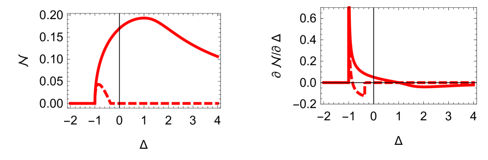
Figure 1: (Color online) Negativity (left) and its derivative with respect to $\Delta$ (right) vs $\Delta$ for nearest neighbor spins (solid line) and next to nearest neighbor spins (dashed line) of the $XXZ$ model.

From Fig. (1), we observe that, for the nearest neighbor spins, the negativity increases monotonously with anisotropy in the region $-1<\Delta<1$, while in the region $\Delta>1$ the negativity decreases as anisotropy increases. And the entanglement reaches the maximal value tt $\Delta=1$. For the next to nearest neighbor spins, only in the region $\Delta\in(-1,-0.358733)$ the entanglement is non-zero. Moreover, the sudden birth of entanglement happens at $\Delta=-1$ both for the nearest and next to nearest neighbor spins. From the right figure one can see that the transition happens also at the critical point $\Delta=-1$.

ii) We take the information deficit to capture the quantum correlation of the $XXZ$ system. In the parameter region $-1<\Delta<1$, the optimal projective measurement bases (II) are obtained at $\theta=\pi/4$ and $\varphi=0$. We have the analytical expression of information deficit for the nearest neighbor spins,

$$\mathcal{I} = \frac{1}{4}\{2(1+\langle\sigma_{i}^{z}\sigma_{i+1}^{z}\rangle)\log(1+\langle\sigma_{i}^{z}\sigma_{i+1}^{z}\rangle)-\sum_{\pm}[2(1\pm\langle\sigma_{i}^{x}\sigma_{i+1}^{x}\rangle)\log(1\pm\langle\sigma_{i}^{x}\sigma_{i+1}^{x}\rangle)$$ (24)

$$- (1-\langle\sigma_{i}^{z}\sigma_{i+1}^{z}\rangle\pm 2\langle\sigma_{i}^{x}\sigma_{i+1}^{x}\rangle)\log(1-\langle\sigma_{i}^{z}\sigma_{i+1}^{z}\rangle\pm 2\langle\sigma_{i}^{x}\sigma_{i+1}^{x}\rangle)]\}.$$

For other regions of $\Delta$, the optimal measurement are given by $\theta=0$ and $\varphi=0$. We have

$$\mathcal{I} = \frac{1}{4}\{\sum_{\pm}[(1-\langle\sigma_{i}^{z}\sigma_{i+1}^{z}\rangle\pm 2\langle\sigma_{i}^{x}\sigma_{i+1}^{x}\rangle)\log(1-\langle\sigma_{i}^{z}\sigma_{i+1}^{z}\rangle\pm 2\langle\sigma_{i}^{x}\sigma_{i+1}^{x}\rangle)$$ (25)

$$- 2(1-\langle\sigma_{i}^{z}\sigma_{i+1}^{z}\rangle)\log(1-\langle\sigma_{i}^{z}\sigma_{i+1}^{z}\rangle)]\}.$$

The analytical expression of information deficit for the next to nearest neighbor spins is in coincidence with the nearest neighbor spins. However, their scales are different (see Fig.2). In fact, the above exact expressions of information deficit are also adapted for quantum discord Dillenschneider2008 .

Figure 2: (Color online) Information deficit (left) for the $XXZ$ model for both nearest (solid line) and next to nearest (dashed line) neighbor spins and its derivative with respect to $\Delta$ (right) vs $\Delta$.

From Fig.(2), we see that the information deficit in the region $\Delta>1$ decreases monotonously with anisotropy $\Delta$ for both the nearest and next to nearest neighbor spins. There are two critical points at $\Delta=-1$ and $1$ in the derivative of information deficit with respect to $\Delta$, showing a kind of quantum phase transitions for the $XXZ$ spin-1/2 chain.

iii) Trace distance discord. For the nearest neighbor spins, the analytical expression of trace distance discord is given by $\mathcal{D}=|\langle\sigma_{i}^{x}\sigma_{i+1}^{x}\rangle|/2$, which is also the formula for the next to nearest neighbor spins.

For the nearest neighbor spins, the trace distance discord increases monotonously with anisotropy in the region $-1<\Delta<0$, while in the region $\Delta\geq 0$, it decreases as anisotropy $\Delta$ increases (see Fig. (3)). A sudden change happens at $\Delta=-1$ both for the nearest and next to nearest neighbor spins, giving rise to quantum phase transitions of the $XXZ$ model.

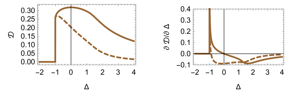
Figure 3: (Color online) Trace distance discord (left) and its derivative with respect to $\Delta$ (right) vs $\Delta$ for the $XXZ$ model for nearest (solid line) and next to nearest (dashed line) neighbor spin.

iv) The analytical formula of the local quantum uncertainty for both nearest and next to nearest neighbor spins can be written as

$$\mathcal{U}=1-\left\{\begin{array}[]{ll}\sqrt{1+\langle\sigma_{i}^{z}\sigma_{i+1}^{z}\rangle}\left(\sqrt{1-\langle\sigma_{i}^{z}\sigma_{i+1}^{z}\rangle+2\langle\sigma_{i}^{x}\sigma_{i+1}^{x}\rangle}+\sqrt{1-\langle\sigma_{i}^{z}\sigma_{i+1}^{z}\rangle-2\langle\sigma_{i}^{x}\sigma_{i+1}^{x}\rangle}\right)&\quad-1<\Delta<1,\cr 1+\langle\sigma_{i}^{z}\sigma_{i+1}^{z}\rangle+\sqrt{(1-\langle\sigma_{i}^{z}\sigma_{i+1}^{z}\rangle)^{2}-4\langle\sigma_{i}^{x}\sigma_{i+1}^{x}\rangle^{2}}&\qquad others.\end{array}\right.$$

Fig. (4) shows that the local quantum uncertainty in the region $\Delta>1$ decreases monotonously. There are two critical points at $\Delta=-1$ and $1$, which show the phase transitions in both the nearest and the next to nearest neighbor spin correlations.

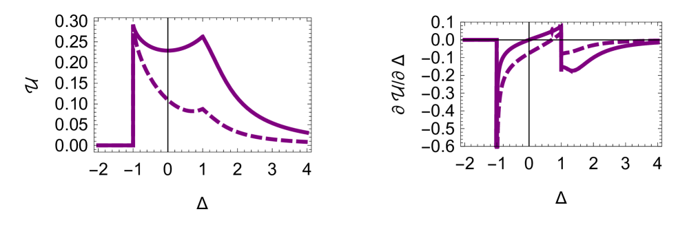
Figure 4: (Color online) Local quantum uncertainty (left) for the $XXZ$ model: the nearest (solid line) and the next to nearest neighbor (dashed line) spins and its derivatives (right) vs $\Delta$.

IV LMG model

We now consider the LMG model Lipkin1965 , which describes a two-level Fermi system $\{|+\rangle,|-\rangle\}$, with each level having degeneracy $g$. The Hamiltonian for LMG model can be written as

$$H=\lambda\sum_{m=1}^{g}\frac{1}{2}(c_{+m}^{\dagger}c_{+m}-c_{-m}^{\dagger}c_{-m})-\frac{1}{2N}\sum_{m,n=1}^{g}(c_{+m}^{\dagger}c_{-m}c_{+n}^{\dagger}c_{-n}+c_{-n}^{\dagger}c_{+n}c_{-m}^{\dagger}c_{+m}),$$ (28)

where the operators $c_{+m}^{\dagger}$ and $c_{-m}^{\dagger}$ create a particle in the upper and lower levels, respectively. Alternatively, the LMG model can be seen as a one-dimensional ring of spin-1/2 particles with an infinite range interaction between pairs. In fact, the Hamiltonian can be rewritten as

$$H=\lambda S_{z}-\frac{1}{N}(S_{x}^{2}-S_{y}^{2}),$$ (29)

with $S_{z}=\sum_{m=1}^{N}\frac{1}{2}(c_{+m}^{\dagger}c_{+m}-c_{-m}^{\dagger}c_{-m})$ and $S_{x}+iS_{y}=\sum_{m=1}^{N}c_{+m}^{\dagger}c_{-m}$ Ring2004 . The LMG model experiences a second-order quantum phase transitions at $\lambda=1$. As $g\rightarrow\infty$, the ground state, as given by the HF approach, reads as

$$|HF\rangle=\prod\limits_{m=1}^{\omega}a_{0m}^{\dagger}|-\rangle,$$ (30)

where the new levels labeled by $0$ and $1$ are governed by the operators

$$a_{0m}^{\dagger} = \cos\alpha\,c_{-m}^{\dagger}+\sin\alpha\,c_{+m}^{\dagger},$$

$$a_{1m}^{\dagger} = -\sin\alpha\,c_{-m}^{\dagger}+\cos\alpha\,c_{+m}^{\dagger}.$$ (31)

In Eq.(IV), $\alpha$ is a variational parameter to be adjusted in order to minimize energy, which is achieved according to the choice

$$\begin{split}\lambda<1\Rightarrow\cos 2\alpha=\lambda,\\ \lambda\geq 1\Rightarrow\alpha=0.\end{split}$$ (32)

Despite being an approximation, the $HF$ ground state provides the exact description of the critical point. The pairwise density operator for general modes $i=(+m)$ and $j=(-n)$ is described as

$$\rho_{i,j}=\left(\begin{array}[]{cccc}\langle M_{i}M_{j}\rangle&0&0&0\cr 0&\langle M_{i}N_{j}\rangle&\langle c_{i}^{\dagger}c_{j}\rangle&0\cr 0&\langle c_{j}^{\dagger}c_{i}\rangle&\langle N_{i}M_{j}\rangle&0\cr 0&0&0&\langle N_{i}N_{j}\rangle\end{array}\right),$$ (37)

where $M_{k}=1-N_{k}$ and $N_{k}=c_{k}^{\dagger}c_{k}$, with $k=i,j$. The Eq. (37) shows a $Z_{2}$ symmetry.

The evaluated matrix elements of $\rho$ for the HF ground state are given by

$$\langle M_{+m}M_{-n}\rangle = \sin^{2}\alpha\cos^{2}\alpha(1-\delta_{mn}),$$

$$\langle M_{+m}N_{-n}\rangle = \cos^{2}\alpha\delta_{mn}+\cos^{4}\alpha(1-\delta_{mn}),$$

$$\langle N_{+m}M_{-n}\rangle = \sin^{2}\alpha\delta_{mn}+\sin^{4}\alpha(1-\delta_{mn}),$$

$$\langle N_{+m}N_{-n}\rangle = \sin^{2}\alpha\cos^{2}\alpha(1-\delta_{mn}),$$

$$\langle c_{+m}^{\dagger}c_{-n}\rangle = \sin\alpha\cos\alpha\delta_{mn},$$

$$\langle c_{-n}^{\dagger}c_{+m}\rangle = \sin\alpha\cos\alpha\delta_{mn}.$$ (38)

Here for $m\neq n$, the density matrix Eq. (37) is diagonal and the state is completely pairwise uncorrelated. On the other hand, for $m=n$, there are quantum correlations between the modes. These correlations vanish for $\lambda>1$, which gives rise to the fully polarized states.

i) Negativity of LMG. We can derive the analytical expression of negativity for the LMG model

$$\mathcal{N}=\frac{1}{2}\sqrt{1-\lambda^{2}}.$$ (39)

ii) Information deficit for LMG. The analytical expression of information deficit for the LMG model has the following form,

$$\mathcal{I}=-\frac{\log\left(\frac{1-\lambda}{4}\right)+\log(\lambda+1)}{2}-\lambda\tanh^{-1}(\lambda)/\ln 2.$$ (40)

Here, the optimal measurement is arrived at $\theta=\phi=0$ for Eq. (II).

iii) By tedious calculation, we have the expressions of trace distance discord for the LMG model,

$$\mathcal{D}=\frac{1}{2}\sqrt{1-\lambda^{2}},$$ (41)

which is the same as the measures negativity.

iv) Local quantum uncertainty for LMG. By straightforward computation, we obtain the analytical expressions of the local quantum uncertainty for LMG,

$$\mathcal{U}=1-\lambda.$$ (42)

From the above analytical results, we see that all of the four kinds of quantum correlations decrease monotonously with $\lambda<1$, see Fig.(5). And in the region $\lambda\geq 1$ the quantum correlations vanishes. One can also observe that the derivatives of the four kind quantum correlations exhibit a signature of the quantum phase transition (see the right figure in Fig. (5).

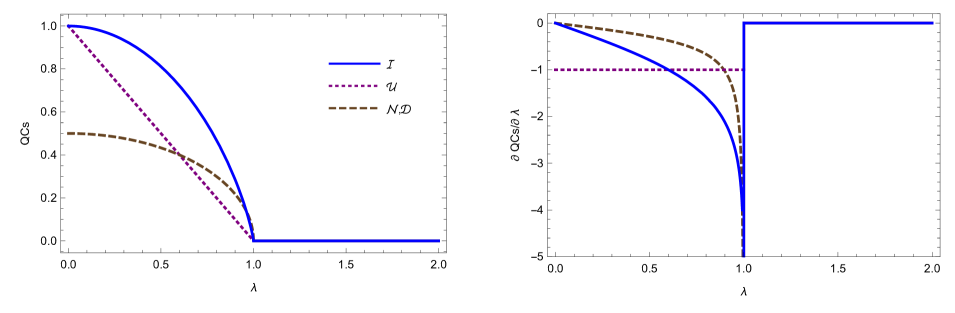
Figure 5: (Color online) All kinds quantum correlations (QCs) and their derivative vs parameter $\lambda$ between modes $(+m)$ and $(-m)$ in the HF ground state of the LMG model.

V Conclusions

We have investigated the behavior of quantum correlations for the Heisenberg $XXZ$ spin-1/2 chain via negativity, information deficit, trace distance discord and local quantum uncertainty. Some properties of the $XXZ$ system are given as follows:

(1) Information deficit and local quantum uncertainty demonstrate the quantum phase transitions at $\Delta=-1$ and $1$. However, the negativity and trace distance discord fail to detect the quantum phase transition at $\Delta=1$.

(2) For the nearest neighbor spins, entanglement and information deficit reach their maximal value at $\Delta=1$. While trace distance discord has the maximal value at $\Delta=0$, and local quantum uncertainty has the maximal value at $\Delta=-1$.

(3) The quantum correlation of the nearest neighbor spins are greater than that of the next to nearest neighbor spins for all the four kinds measures.

We have also considered quantum correlations in the Hartree-Fock ground state of the Lipkin-Meshkov-Glick model. All the four quantum correlation measures has been analytically worked out. The behaviors for both $XXZ$ spin-1/2 chains and LMG model have been discussed. It is shown that all of the quantum correlation measures exhibit signatures of the quantum phase transitions.

We have studied the ability of quantum correlations to spotlight critical points of quantum phase transitions for an infinite spin chain described by the $XXZ$ model, in terms of four distinct types of quantum correlations between pairs of nearest and next to nearest neighbor spins. All the measures of these quantum correlations show quantum phase transitions at $\Delta=-1$ for both the nearest and next to nearest neighbor spins. However, the information deficit and local quantum uncertainty exhibit one more singularity at the critical point $\Delta=1$. It can be seen that information deficit and local quantum uncertainty are better in studying the critical points for the $XXZ$ spin system.

Our work highlights the type of quantum correlations involved at the quantum phase transition of the $XXZ$ system and LMG model. These measures show the ways to explore quantum phase transition in condensed matter physics. These quantities are important tools in the investigation of quantum phase transitions in realistic experimental scenarios. The approach can be also used to explore quantum phase transitions in other physical systems.

References

• (1) L. Amico, R. Fazio, A. Osterloh, and V. Vedral, Rev. Mod. Phys. 80, 517 (2008).
• (2) R. Horodecki, P. Horodecki, M. Horodecki, and K. Horodecki, Rev. Mod. Phys. 81, 865 (2009).
• (3) Z. Merali, Nature 474, 24 (2011).
• (4) K. Modi, A. Brodutch, H. Cable, T. Paterek, and V. Vedral, Rev. Mod. Phys. 84, 1655 (2012).
• (5) G. Adesso, T. R. Bromley, and M. Cianciaruso, J. Phys. A: Math. Theor. 49, 473001 (2016).
• (6) H. Ollivier and W. H. Zurek, Phys. Rev. Lett. 88, 017901 (2001).
• (7) J. Oppenheim, M. Horodecki, P. Horodecki, and R. Horodecki, Phys. Rev. Lett. 89, 180402 (2002).
• (8) B. Dakić, V. Vedral, and Č. Brukner, Phys. Rev. Lett. 105, 190502 (2010).
• (9) F. Ciccarello, T. Tufarelli, and V. Giovannetti, New J. Phys. 16, 013038 (2014).
• (10) D. Girolami, T. Tufarelli, and G. Adesso, Phys. Rev. Lett. 110, 240402 (2013).
• (11) T. Werlang, C. Trippe, G. A. P. Ribeiro, and G. Rigolin, Phys. Rev. Lett. 105, 095702 (2010).
• (12) T. Werlang, G. A. P. Ribeiro, and G. Rigolin, Phys. Rev. A 83, 062334 (2011).
• (13) Y.-C. Li and H.-Q. Lin, Phys. Rev. A 83, 052323 (2011).
• (14) L. Justino and T. R. de Oliveira, Phys. Rev. A 85, 052128 (2012).
• (15) A. L. Malvezzi, G. Karpat, B. Çakmak, F. F. Fanchini, T. Debarba, and R. O. Vianna, Phys. Rev. B 93, 184428 (2016).
• (16) M. Sarandy, Phys. Rev. A 80, 022108 (2009).
• (17) G. Vidal and R. F. Werner, Phys. Rev. A 65, 032314 (2002).
• (18) M. Horodecki, P. Horodecki, R. Horodecki, J. Oppenheim, A. Sen(De), U. Sen, and B. Synak-Radtke, Phys. Rev. A 71, 062307 (2005).
• (19) A. Streltsov, H. Kampermann, and D. Bruß, Phys. Rev. Lett. 106, 160401 (2011).
• (20) B.-L. Ye, Y.-K. Wang, and S.-M. Fei, Int. J. Theor. Phys. 55, 2237 (2016).
• (21) E. P. Wigner and M. M. Yanase, Proc. Natl. Acad. Sci. U.S.A. 49, 910 (1963).
• (22) S. Luo, Phys. Rev. Lett. 91, 180403 (2003).
• (23) M. Takahashi, Thermodynamics of one-dimensional solvable models, Cambridge University Press (2005).
• (24) M. Shiroishi and M. Takahashi, J. Phys. Soc. Jpn. 74, 47 (2005).
• (25) M. Takahashi, G. Kato, and M. Shiroishi, J. Phys. Soc. Jpn. 73, 245 (2004).
• (26) G. Kato, M. Shiroishi, M. Takahashi, and K. Sakai, J. Phys. A: Math. Gen. 37, 5097 (2004).
• (27) G. Kato, M. Shiroishi, M. Takahashi, and K. Sakai, J. Phys. A: Math. Gen. 36, L337 (2003).
• (28) R. Dillenschneider, Phys. Rev. B 78, 224413 (2008).
• (29) H. J. Lipkin, N. Meshkov, and A. J. Glick, Nucl. Phys. 62, 188 (1965).
• (30) P. Ring and P. Schuck, The nuclear many-body problem, Springer Science & Business Media (2004).